IN DEGREE PROJECT MEDICAL ENGINEERING,SECOND CYCLE, 30 CREDITS

, STOCKHOLM SWEDEN 2016

Segmentation of Cone Beam CT in Stereotactic Radiosurgery

AWAIS ASHFAQ

KTH ROYAL INSTITUTE OF TECHNOLOGYSCHOOL OF TECHNOLOGY AND HEALTH

This master thesis was performed in the Research and Physics Department at Elekta Instrument AB, Stockholm and School of Technology and Health at KTH Royal Institute of Technology.

Segmentation of Cone Beam CT in

Stereotactic Radiosurgery

Awa i s Ash f aq

Master of Science Thesis in Medical Engineering Advanced level (second cycle), 30 credits

Supervisor at KTH: Asst Prof Pawel Herman Supervisor at Elekta: Jonas Adler

Examiner: Dr. Mats Nilsson School of Technology and Health

TRITA-STH. EX 2016:104

Royal Institute of Technology KTH STH

SE-141 86 Flemingsberg, Sweden http://www.kth.se/sth

Abstract

C-arm Cone Beam CT (CBCT) systems – due to compact size, flexible geometry and low radiation exposure – inaugurated the era of on-board 3D image guidance in therapeutic and surgical procedures. Leksell Gamma Knife Icon by Elekta introduced an integrated CBCT system to determine patient position prior to surgical session, thus advancing to a paradigm shift in facilitating frameless stereotactic radiosurgeries. While CBCT offers a quick imaging facility with high spatial accuracy, the quantitative values tend to be distorted due to various physics based artifacts such as scatter, beam hardening and cone beam effect. Several 3D reconstruction algorithms targeting these artifacts involve an accurate and fast segmentation of craniofacial CBCT images into air, tissue and bone. The objective of the thesis is to investigate the performance of deep learning based convolutional neural networks (CNN) in relation to conventional image processing and machine learning algorithms in segmenting CBCT images. CBCT data for training and testing procedures was provided by Elekta. A framework of segmentation algorithms including multilevel automatic thresholding, fuzzy clustering, multilayer perceptron and CNN is developed and tested against pre-defined evaluation metrics carrying pixel-wise prediction accuracy, statistical tests and execution times among others. CNN has proven its ability to outperform other segmentation algorithms throughout the evaluation metrics except for execution times. Mean segmentation error for CNN is found to be 0.4% with a standard deviation of 0.07%, followed by fuzzy clustering with mean segmentation error of 0.8% and a standard deviation of 0.12%. CNN based segmentation takes 500s compared to multilevel thresholding which requires ~1s on similar sized CBCT image. The present work demonstrates the ability of CNN in handling artifacts and noise in CBCT images and maintaining a high semantic segmentation performance. However, further efforts targeting CNN execution speed are required to utilize the segmentation framework within real-time 3D reconstruction algorithms. Keywords: Cone Beam CT, Convolutional Neural Networks, Image Segmentation, Leksell Gamma Knife Icon, Deep Learning.

Sammanfattning

C-arm Cone Beam CT (CBCT) system har tack vare sitt kompakta format, flexibla geometri och låga strålningsdos startat en era av inbyggda 3D bildtagningssystem för styrning av terapeutiska och kirurgiska ingripanden. Elektas Leksell Gamma Knife Icon introducerade ett integrerat CBCT-system för att bestämma patientens position för operationer och på så sätt gå in i en paradigm av ramlös stereotaktisk strålkirurgi. Även om CBCT erbjuder snabb bildtagning med hög spatiel noggrannhet så tenderar de kvantitativa värdena att störas av olika artefakter som spridning, beam hardening och cone beam effekten. Ett flertal 3D rekonstruktionsalgorithmer som försöker reducera dessa artefakter kräver en noggrann och snabb segmentering av kraniofaciala CBCT-bilder i luft, mjukvävnad och ben. Målet med den här avhandlingen är att undersöka hur djupa neurala nätverk baserade på faltning (convolutional neural networks, CNN) presterar i jämförelse med konventionella bildbehandlings- och maskininlärningalgorithmer för segmentering av CBCT-bilder. CBCT-data för träning och testning tillhandahölls av Elekta. Ett ramverk för segmenteringsalgorithmer inklusive flernivåströskling (multilevel automatic thresholding), suddig klustring (fuzzy clustering), flerlagersperceptroner (multilayer perceptron) och CNN utvecklas och testas mot fördefinerade utvärderingskriterier som pixelvis noggrannhet, statistiska tester och körtid. CNN presterade bäst i alla metriker förutom körtid. Det genomsnittliga segmenteringsfelet för CNN var 0.4% med en standardavvikelse på 0.07%, följt av suddig klustring med ett medelfel på 0.8% och en standardavvikelse på 0.12%. CNN kräver 500 sekunder jämfört med ungefär 1 sekund för den snabbaste algorithmen, flernivåströskling på lika stora CBCT-volymer. Arbetet visar CNNs förmåga att handera artefakter och brus i CBCT-bilder och bibehålla en högkvalitativ semantisk segmentering. Vidare arbete behövs dock för att förbättra presetandan hos algorithmen för att metoden ska vara applicerbar i realtidsrekonstruktionsalgorithmer. Nyckelord: Cone Beam CT, neurala nätverk baserade på faltning, bildsegmentering, Leksell Gamma Knife Icon, Djup inlärning.

To the One who gives me life

Table of Contents

1. Introduction ........................................................................................... 1

1.1 Problem Statement .................................................................................................. 2 1.2 Aim .......................................................................................................................... 3 1.3 Thesis Layout ........................................................................................................... 3

2. Methods ................................................................................................. 4

2.1 Convolutional Neural Networks ........................................................................... 4 2.1.1 Training ............................................................................................................. 4 2.1.2 Implementation ................................................................................................ 11 2.1.3 Testing ............................................................................................................. 11

2.2 Other Algorithms ............................................................................................... 13 2.2.1 Features Selection ............................................................................................ 13 2.2.2 Modified Fuzzy C-means ................................................................................. 14

2.3 Evaluation Metrics ............................................................................................. 15 3. Results ................................................................................................. 16

3.1 Two Sample T-Test ............................................................................................... 16 3.2 Confusion Matrix ................................................................................................... 17 3.3 ROI error ............................................................................................................... 19 3.4 Visualization .......................................................................................................... 20

4. Discussion ............................................................................................. 22

4.1 Performance ........................................................................................................... 22 4.2 Limitations ............................................................................................................. 24

5. Conclusion ............................................................................................ 26 Appendix A: Background and Literature Review ....................................... 27

A.1 Computed Tomography ........................................................................................ 27 A.2 Cone Beam Computed Tomography ..................................................................... 28 A.3 CBCT System at Elekta ....................................................................................... 29 A.4 CBCT Artifacts ..................................................................................................... 31 A.5 CBCT Denoising Methods .................................................................................... 33 A.6 Segmentation ......................................................................................................... 36

Appendix B: Image Processing and Segmentation ..................................... 37

B.1 Image Filtering ...................................................................................................... 37 B.2 Automatic Thresholding ........................................................................................ 38 B.3 K-means ................................................................................................................ 38 B.4 Fuzzy C-means ...................................................................................................... 38 B.5 Mean Shift ............................................................................................................. 39 B.6 Multilayer Perceptron ........................................................................................... 39 B.7 Convolutional Neural Networks ............................................................................ 40

References ................................................................................................... 42

i

List of Figures

Figure 1.1: The Leksell Gamma Knife Icon....................................................................... 1 Figure 2.1: Steps involved in preparation of training images and labels ........................... 5 Figure 2.2: A 3D illustration of the stereotactic head frame ............................................. 6 Figure 2.3: Extracting patches around edge pixels............................................................ 6 Figure 2.4: Patch generation around edge pixels .............................................................. 7 Figure 2.5: Block diagram of the implemented CNN ........................................................ 8 Figure 2.6: Validation set assisting in avoiding over-fitting. ........................................... 11 Figure 2.7: Block diagram for parallel test data processing ............................................ 12 Figure 2.8: A slice from craniofacial probabilistic maps .................................................. 13 Figure 2.9: Modified fuzzy C-means framework .............................................................. 14 Figure 3.1: Box plots showing statistical distribution of prediction accuracy ................ 18 Figure 3.2: 5 Regions of interest (L-R) in CBCT images. ............................................... 19 Figure 3.3: Bar graph showing pixel prediction error in 5 ROI's .................................... 19 Figure 3.4: Visual comparison of different segmentation algorithms. ............................. 21 Figure 4.1: Bone information per craniofacial CBCT slice .............................................. 22 Figure 4.2: An illustration of beam hardening in CT images .......................................... 25 Figure A.1: Comparison of conventional fan beam CT and CBCT systems................... 28 Figure A.2: Elekta CBCT scanner .................................................................................. 30 Figure A.3: Basic artifacts in CBCT images ................................................................... 32 Figure A.4: Basic steps in CBCT image creation ............................................................ 34 Figure A.5: Iterative reconstruction flowchart ................................................................ 35 Figure A.6: Typical framework for a scatter correction method ..................................... 35 Figure B.1: Automatic thresholding ................................................................................ 38 Figure B.2: Multilayer perceptron ................................................................................... 39 Figure B.3: Features in deep learning in context of images. ........................................... 40

ii

List of Abbreviations

ANN Artificial Neural Network CBCT Cone Beam Computed Tomography CNN Convolutional Neural Network CPU Central Processing Unit CT Computed Tomography CUDA Compute Unified Device Architecture cuDNN CUDA Deep Neural Network library DICOM Digital Imaging and Communications in Medicine DL Deep Learning FBP Filtered Backprojection FCM Fuzzy C Means GPU Graphical Processing Unit IGRT Image Guided Radiation Therapy LMA Levenberg-Marquardt Algorithm MFCM Modified Fuzzy C-means ML Machine Learning MLP Multilayer Perceptron MR Magnetic Resonance NLM Non-Local Means ReLU Rectified Linear Unit RMSE Root Mean Square Error ROI Region of Interest SVM Support Vector Machine

iii

1. Introduction

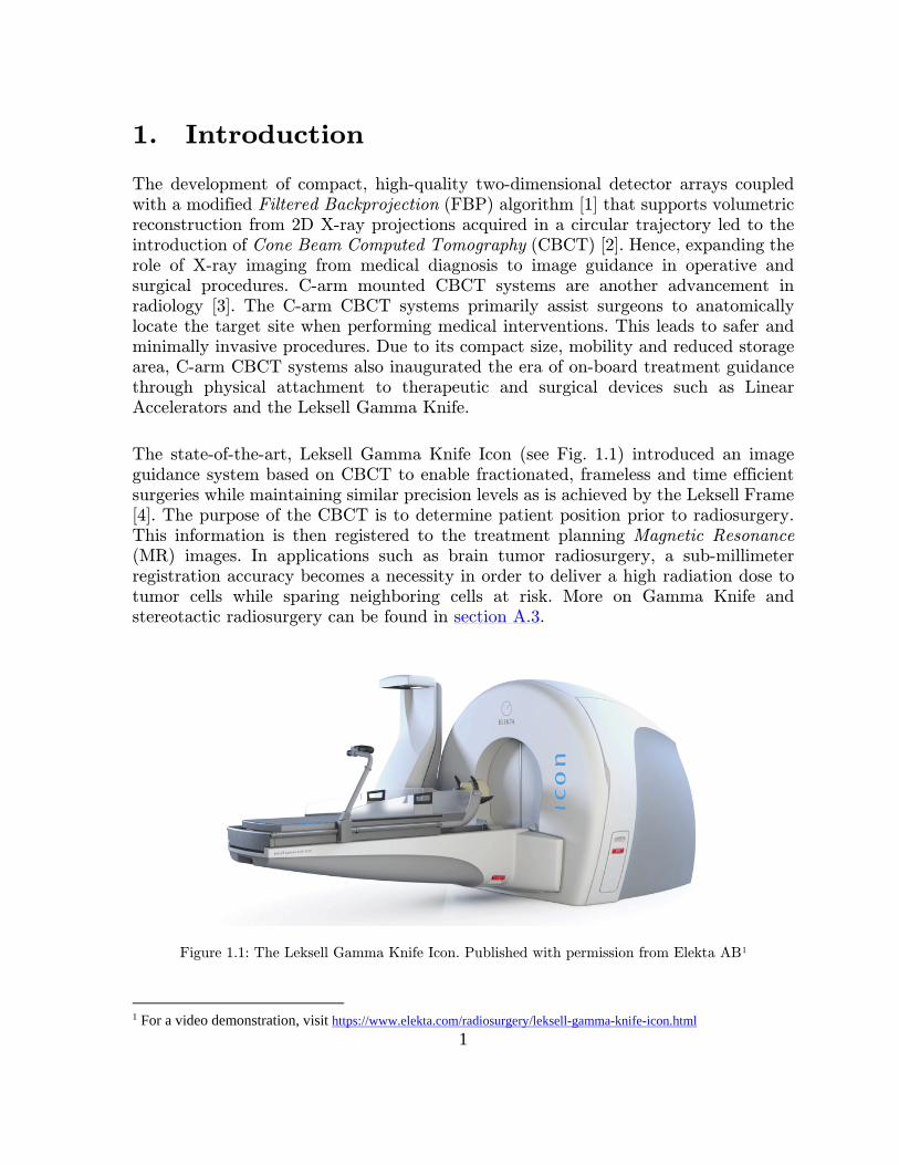
The development of compact, high-quality two-dimensional detector arrays coupled with a modified Filtered Backprojection (FBP) algorithm [1] that supports volumetric reconstruction from 2D X-ray projections acquired in a circular trajectory led to the introduction of Cone Beam Computed Tomography (CBCT) [2]. Hence, expanding the role of X-ray imaging from medical diagnosis to image guidance in operative and surgical procedures. C-arm mounted CBCT systems are another advancement in radiology [3]. The C-arm CBCT systems primarily assist surgeons to anatomically locate the target site when performing medical interventions. This leads to safer and minimally invasive procedures. Due to its compact size, mobility and reduced storage area, C-arm CBCT systems also inaugurated the era of on-board treatment guidance through physical attachment to therapeutic and surgical devices such as Linear Accelerators and the Leksell Gamma Knife.

The state-of-the-art, Leksell Gamma Knife Icon (see Fig. 1.1) introduced an image guidance system based on CBCT to enable fractionated, frameless and time efficient surgeries while maintaining similar precision levels as is achieved by the Leksell Frame [4]. The purpose of the CBCT is to determine patient position prior to radiosurgery. This information is then registered to the treatment planning Magnetic Resonance (MR) images. In applications such as brain tumor radiosurgery, a sub-millimeter registration accuracy becomes a necessity in order to deliver a high radiation dose to tumor cells while sparing neighboring cells at risk. More on Gamma Knife and stereotactic radiosurgery can be found in section A.3.

Figure 1.1: The Leksell Gamma Knife Icon. Published with permission from Elekta AB1

1 For a video demonstration, visit https://www.elekta.com/radiosurgery/leksell-gamma-knife-icon.html 1

1.1 Problem Statement

CBCT offers a quick imaging facility with high spatial accuracy, yet the quantitative values tend to be distorted due to various artifacts such as photon scattering, beam hardening and photon starvation. This results in a sub-optimal registration performance of the planning MR and stereotactic CBCT images resulting in a less accurate positioning of the target site. Most of the existing software methods used for artifact reduction in CBCT [5-9] require a fast and accurate segmentation of the volume into different materials. See section A.5.2 for details. Automated image segmentation is a fundamental problem in medical image analysis. The applications include contouring organs, lesion (tumor) detections, dose calculations, noise reduction etc. There are three broad categories of segmentation methods.

(i) Segmentation based on local information. These algorithms tend to work from an image processing viewpoint. They include image analysis based morphological and thresholding operations [10]. These methods are sensitive to image noise and non-uniform object textures among others. (ii) Segmentation based on a priori information. Contrary to local information, these are high-level methods that make use of prior information of the expected volume and adapt it to the actual volume. They include deformable models and atlas-based segmentations [11-13]. There are two main drawbacks of these methods. First, they require a rich database for constructing atlases. Unlike MR images, the availability of CBCT data is sparse. Second, these methods require a smooth transformation between expected and actual volumes. Tumors and other pathological conditions may disrupt this transformation. (iii) Segmentation based on Machine Learning (ML) techniques. These methods have recently shown huge success in medical image segmentation inclined towards MR and CT images [14]. These methods make use of supervised learning principles where a set of training data (hand-engineered input features) and corresponding labels are fed into a network for training under a certain ML algorithm. More on ML algorithms can be found in [15]. A major drawback of these so called hand-crafted training features is that they are unable to extract salient information from the data. As a result their performance varies from dataset to dataset. Contrary to such segmentation methods that are dependent on feature engineering, deep learning networks directly extract hierarchical features specialized for the training data [16]. Deep learning based methods for medical image segmentation have shown to outperform the traditional feature based methods on MR images [17, 18]. However, to the best of our knowledge, these methods have not yet been tested on CBCT images.

2

1.2 Aim

The objective of the thesis is to develop and implement a deep learning based convolutional neural network [19] for de-noising CBCT volumes through semantic

segmentation – voxel classification into air, soft tissue or bone. It is aimed at investigating whether deep learning based convolutional neural networks surpass the conventional image processing and ML methods in segmenting noisy CBCT images given the following evaluation metrics (see section 2.3 for details)

i. Two-sample T-test p-values ii. Confusion matrix iii. Execution time iv. Region of interest (ROI) error v. Visual inspection

It is hypothesized that CNN shall outperform conventional image processing and ML methods in segmenting noisy CBCT volumes. The hypothesis is based on following grounds:

1. Deep learning models tend to extract high-level abstraction within data which make them less sensitive to image noise.

2. Deep architectures have shown promising segmentation results on MR images [17, 18, 20].

1.2.1 Scientific Contribution

CBCT is widely used as a treatment planning tool in implant dentistry and as a patient positioning tool in image guided radiation therapy [3]. It offers a simpler geometry and also less radiation exposure compared to conventional CT [21]. This

work addresses an important limitation of CBCT – poor image contrast – which has been a prime research area in the past decade [22]. The current work scope focuses on semantic segmentation aimed at noise reduction in CBCT, however, similar framework may be extended to other applications such as dose calculation. The current work also introduces the novelty of using CNN in segmenting CBCT images. It highlights necessary areas to consider when using deep learning architectures for semantic segmentation of medical images. Last but not least, the present work features the ability of CNN in resisting noise artifacts when extracting salient features from the images. The idea of processing noisy images in CNN is unique in its way because CNN

- unlike deep encoder networks – has found most of its application in image classification and object recognition domains.

1.3 Thesis Layout

Chapter 2 and 3 describes the implementation of methods and results respectively. Chapter 4 discusses the proposed results, challenges and possible improvements. Appendix A covers the State of the Art in CBCT and its applications. Appendix B covers a revision of basic image processing and segmentation techniques.

3

2. Methods

This chapter shall describe and motivate the steps involved to develop the segmentation model for CBCT images.

2.1 Convolutional Neural Networks

Convolutional Neural Networks (CNN) belong to the group feed-forward Artificial Neural Networks where the connectivity pattern between different layers is inspired by the connectivity in the animal visual cortex. See section B.7 for details on CNN.

2.1.1 Training

The training of a CNN is carried out in a supervised fashion. This means that for every input image we require a true label. These image-label pairs are stored in a training set. The training process was divided into following key steps: I. Data Preparation Training data and labels were generated in the following order: (see Fig. 2.1)

i. Craniofacial real CT data was provided by Elekta Instruments, Stockholm. All CT images had a stereotactic frame attached to the head which needed to be removed from the images in order to proceed with the segmentation method (see Fig. 2.2). This dataset has over 1000 3D CT images of mixed gender and age

groups. All images were of size 512x512x𝑆𝑆, where 𝑆𝑆 is the number of slices

ascending to the top of the head. 𝑆𝑆 varies between 100 and 200 throughout the dataset. The voxel size is 0.5x0.5x1.0mm3

ii. After frame removal, one CT image was randomly selected to be a template (size: 512x512x154) to provide a common frame of reference. A unimodal intensity-based rigid registration was performed to geometrically align every other CT image one at a time with the template. Rigid registration consists of translational and rotational transformations to align images with the template. This operation also results in every input image of size equivalent to the template size.

iii. Next, hard segmentation of registered CT images into bone, tissue and air regions was performed using multi-level thresholding [23]. These are training labels.

iv. CBCT projections were then acquired using Elekta's proprietary algorithm involving density calculations from CT Data F, segmented CT Data G and energy spectrum of the Elekta Icon CBCT.

v. Finally, CBCT projections were reconstructed using Conjugate Gradient Least Square (CGLS) technique in the Operator Discretization Library (ODL) package2. These are the training images.

40 CBCT images and corresponding labels were generated following the method in Fig. 2.1. 20 images were used for training the CNN and the remaining were used for testing.

2 Available at https://github.com/odlgroup/odl 4

G. Multi-Class Thresholding

E. Apply mask to CT volume

I. 3D CBCT

H. CBCT Projections

Training Labels

Training Images

F. CT Registration

D. Extract largest 3D contiguous region

A. 3D CT

B. Otsu Thresholding

C. 3D Filling

Figure 2.1: An illustration of steps involved in preparation of training images and labels. A. Craniofacial CT data provided by Elekta, Stockholm. B. After applying Otsu Thresholding at 30%. C. After 3D morphological filling operation with holes. D. After extracting the largest connected region in the volume with a 3D connectivity of 26. E. After applying the mask generated in D to A. F. After performing rigid registration with a CT template. G. After applying multi-class thresholding on F. In the current work a voxel may have one of the three training labels: Air = 0; Tissue = 1; Bone = 2. H. Generate CBCT projections using F and G. (Beyond thesis scope: provided by Elekta) I. 3D reconstruction. (Beyond thesis scope: provided by Elekta)

5

II Generate Training Set The training set was at first generated by extracting a 2D patch of size 33x33 centered on every pixel in the CBCT image. Each input image (also known as a patch) corresponds to a single label that belongs to the center pixel of the patch. In general, craniofacial CBCT images have far more air pixels than tissue pixels which are in turn far more than bone pixels. In order to have an optimal training, it is important to incorporate approximately equal number of samples of every class in the training set [24]. A common solution is to isolate bone, tissue and air samples and randomly sort equal number of samples from them. However, a novel approach using Canny Edge detection [25] was implemented to generate a balanced training set. There are two advantages of this approach.

1. Edge pixels are non-trivial because they directly influence the anatomy in the image.

2. Patches around edge voxels, possess a structure which speeds up the learning process (see Fig. 2.3)

Patches around edge voxels only were used for training the CNN. Fig. 2.4 shows different variants of patch sizes attempted during the thesis.

C

B

A

Figure 2.2: A 3D illustration of the stereotactic head frame before and after removal. Metallic screws piercing through patient's head can be seen in the frame-removed image.

Figure 2.3: Extracting patches around edge voxels. Random voxel sampling often results in patches with no structural information (A). Hence, voxel pixels were determined (B) and patches only around edge voxels were captured (C)

6

III. CNN Architecture A usual convention for implementing CNN is to begin with a convolution block followed a spatial pooling block, non-linearity function and a fully connected layer (see section B.7 for details). It is a feed-forward network which means that there are no backward connections in the network. A feed-forward network can be taken as a

stream of linearly stacked non-linear functions.

𝑓𝑓(𝑥𝑥) = �𝑓𝑓𝐿𝐿,𝑤𝑤𝐿𝐿 ∘ … ∘ 𝑓𝑓2,𝑤𝑤2 ∘ 𝑓𝑓1,𝑤𝑤1�(𝑥𝑥) Each functional block 𝑓𝑓𝑙𝑙,𝑤𝑤𝑙𝑙 takes an input 𝑥𝑥𝑙𝑙 along with some parameters 𝑤𝑤𝑙𝑙 to compute

an output 𝑥𝑥𝑙𝑙+1 and the computations carry on until the last stacked function 𝑓𝑓𝐿𝐿 is computed. It must be clear that only 𝑥𝑥 = 𝑥𝑥1 is the actual input image passed to the first computation block. The rest of the blocks get intermediate feature maps. Fig. 2.5 explains the overall architecture of the proposed CNN using case-1 in Fig. 2.4. In this

implementation 𝑥𝑥1 is a 2D square patch and has a single label belonging to the center pixel of the patch. The output of the proposed architecture can be written as

𝑦𝑦 = �𝑠𝑠 ∘ 𝑓𝑓2,𝑤𝑤4 ∘ 𝑅𝑅 ∘ 𝑓𝑓1,𝑤𝑤3 ∘ 𝑅𝑅 ∘ 𝑝𝑝2,𝑎𝑎2 ∘ 𝑐𝑐2,𝑤𝑤2 ∘ 𝑅𝑅 ∘ 𝑝𝑝1,𝑎𝑎1 ∘ 𝑐𝑐1.𝑤𝑤1�(𝑥𝑥1) 𝑤𝑤ℎ𝑒𝑒𝑒𝑒𝑒𝑒 𝑐𝑐𝑛𝑛, 𝑝𝑝𝑛𝑛 and 𝑓𝑓n are the 𝑛𝑛𝑡𝑡ℎconvolution, pooling and fully connected blocks respectively.

𝑅𝑅 and 𝑠𝑠 are the ReLU and softmax operator respectively.

𝑤𝑤𝑛𝑛 are the weight vectors corresponding to convolution or fully connected blocks.

𝑎𝑎𝑛𝑛 is the pooling window of the 𝑛𝑛𝑡𝑡ℎ pooling block.

y is the posterior probability vector of size 1 x 3.

x

y

(1)

(2)

Figure 2.4: Patch generation around edge voxels. Case 1 – is a 2D patch extracted around the edge voxel of interest in the x-y plane. Case 2 – are 3 2D patches extracted around the edge voxel of interest in the x-y, x-z and y-z plane. Case 3 – is a cubic patch extracted around the edge voxel of interest.

z

Pre-processing

Gaussian Filtering Edge Detection

Edge Image 512x512x154

Patch preparation

i. 2D patch ii. Tri-patch

iii. Cubic patch

Case III 33x33x33

Case II 33x33x3

Case I 33x33x1

Input Image 512x512x154

7

Figure 2.5: Block diagram of the implemented CNN

ReLU

ReLU

Feature Maps 29x29x20

Input 33x33

Feature Maps 14x14x1x20

2D Max Pooling

Stride: 2

2D Convolution

5x5x1x20

2D Max Pooling

Stride: 2

Feature Maps 10x10x32

2D Convolution

5x5x20x32

Feature Maps 14x14x20

Feature Maps 5x5x32

Reshape

Feature Maps 5x5x32

Fully Connected

ReLU

Fully Connected

Fully Connected

800x1

512x1

512x1

3x1

Categorical Probability

Distributions

Softmax Loss

8

IV. Training Objective The computations are performed in two modes. In the forward mode, posterior

probabilities 𝑦𝑦 are calculated according to Eq. 2. The posterior probabilities are then compared with the ground truth or labels. The objective of the training algorithm is

to minimize the dissimilarity or error between 𝑦𝑦 and the ground truth. The error

function 𝐸𝐸 is given by cross entropy for a 1-of-𝐾𝐾 coding scheme [15].

𝐸𝐸(𝑊𝑊) = −�𝑁𝑁

𝑖𝑖=1

�𝑡𝑡𝑖𝑖𝑖𝑖ln 𝑆𝑆𝑖𝑖(𝑥𝑥𝑖𝑖 ,𝑊𝑊)𝐾𝐾

𝑖𝑖=1

𝑤𝑤ℎ𝑒𝑒𝑒𝑒𝑒𝑒 𝑊𝑊 is the weight vector.

𝑁𝑁 is the batch size – see VIII of this section for details.

𝑡𝑡𝑖𝑖𝑖𝑖 is the label that 𝑖𝑖 th input image belongs to the 𝑘𝑘th class.

𝑆𝑆 is the softmax operator that returns the probability of the 𝑖𝑖th image to the 𝑘𝑘th class.

Since, the only tunable parameters in Eq. 2 are the weights 𝑤𝑤𝑛𝑛, the error minimization problem can be stated as:

𝑤𝑤1∗,𝑤𝑤2∗,𝑤𝑤3∗,𝑤𝑤4∗ = 𝑎𝑎𝑒𝑒𝑎𝑎𝑎𝑎𝑖𝑖𝑛𝑛𝑤𝑤1,𝑤𝑤2,𝑤𝑤3,𝑤𝑤4 � 𝐸𝐸(𝑥𝑥,𝑇𝑇)∈𝐷𝐷

(𝑊𝑊)

𝑤𝑤ℎ𝑒𝑒𝑒𝑒𝑒𝑒 𝐸𝐸 is the error function between the posterior probabilities 𝑦𝑦 and true label 𝑇𝑇 𝐷𝐷 is the set of training data V. Backpropagation The algorithm used to estimate the optimum weights leading to minimum error as in Eq. 4 is known as backpropagation. It is basically a method of computing gradients with recursive application of chain rule. Mathematical description of the algorithm can be found in [26]. It is a gradient descent algorithm in which the weights are trained to

update the value of 𝐸𝐸 in the direction of negative gradient –downhill - to find a global minima on the error surface. The standard gradient descent algorithm updates the

parameter 𝑊𝑊 of the objective function 𝐸𝐸 (Eq. 3) as

𝑊𝑊𝑛𝑛𝑛𝑛𝑤𝑤 = 𝑊𝑊𝑜𝑜𝑙𝑙𝑜𝑜 − 𝜂𝜂 ∗ ∇𝑊𝑊(𝐸𝐸) 𝑤𝑤ℎ𝑒𝑒𝑒𝑒𝑒𝑒 ∇𝑊𝑊(𝐸𝐸) is the error gradient w.r.t weights.

𝜂𝜂 is the Learning rate.

(5)

(4) (4)

(3)

9

VI. Learning Rate Learning rate governs how fast or slow the network converges towards the global minima. A high learning step may surpass the error minima and lead to unstable learning. A small learning step leads to slow convergence and more processing time. To overcome this, learning rate is set to a high value in the beginning and is gradually decreased as the algorithm progresses. In the current implementation a learning rate of 0.1 was used with a decrement factor of 2 after every 50 iterations.

VII. Momentum Momentum is used to avoid the network getting stuck in a local minima as we descent the error surface. The value of momentum relates to the level of contribution we add to our learning from a previous weight change. Using momentum in CNN also aids in having a smaller learning rate which is necessary for stable learning. In the current

implementation a momentum (𝛼𝛼) of 0.9 was used.

𝑊𝑊𝑛𝑛+1 = 𝑊𝑊𝑛𝑛 − 𝜂𝜂 ∗ ∇𝑊𝑊𝑛𝑛(𝐸𝐸) + 𝛼𝛼(𝑊𝑊𝑛𝑛 −𝑊𝑊𝑛𝑛−1) VIII. Batch Size There are two ways to update the weights in CNN. In serial or online update, images are fed one at a time to the CNN. The image is processed through all the network blocks; error is calculated; and the weights are updated in the direction of negative error gradient. This method has two drawbacks. First, it requires high computation time. Second, it is sensitive to noise as a single noisy image may corrupt the weights of the network. To avoid this, parallel or batch training is used. In batch training input images are grouped together before feeding to the CNN. All computations are performed in a parallel manner and cumulative error of the entire group is calculated which is then back-propagated to update the weights. The number of images sent to the CNN at one time is called the batch size. A higher batch size requires larger parallel

computation memory. In the current implementation, a batch size of 500 was used –

which is symbolized as 𝑁𝑁 in Eq. 3 IX. Validation Set Since the network is allowed training for a given number of iterations, it is likely to lose its generalization ability by overfitting on the training images [27]. In order to avoid over-fitting, 10% of the training images were included in an independent validation set. During every iteration and after the weight update; the validation set was fed to the CNN and the error was calculated. The training error and validation errors were plotted as shown in Fig. 2.6. As the validation set is independent of the training set, it offers a good measure of the generalization ability of the network. No weight update is done using the validation error.

(6)

10

2.1.2 Implementation

Compute Unified Device Architecture (CUDA) is a parallel computing platform developed by NVIDIA [28]. It utilizes the multi-core flexibility of modern day GPU's enabling data processing in a parallel manner rather serially on CPU's. This results in an exceptionally fast computation speed on big data processing applications. CUDA supports C, C++ and Fortran programming languages. Matlab supports CUDA enabled NVIDIA GPU's in its parallel processing toolbox. Since speed is a big concern in the current segmentation problem, the implemented methods make use of the GPU architecture using CUDA libraries. Matlab, Microsoft Visual Studio and Enthought Canopy were used as programming environments. Matconvnet library was used for implementing CNN [26].

2.1.3 Testing

After determining the optimal weights, CNN is frozen and no further weight update takes place. Testing the CNN with an input CBCT image of size (512 x 512 x 154) involves two key steps. First, patch generation (Fig. 2.4) for every pixel in the input

image. Second, computing 𝑦𝑦 (Eq. 2) for every patch. The former step was performed using parallel CPU threads. Each thread gets a 2D image slice (512 x 512) and computes patches (33 x 33 x 262144). Next, one thread at a time requests for GPU

control and 𝑦𝑦′𝑠𝑠 are computed in a batch-wise manner. Based on maximum class probability, every patch is assigned a single label. Once all patches from a single slice are labelled, the GPU control is transferred to the next CPU thread which by now has generated patches from the next slice in queue. Fig. 2.7 illustrates the parallel test architecture.

Figure 2.6: An illustration of how validation set assists in avoiding over-fitting. The arrows mark possible training termination points.

11

Figure 2.7: Block diagram for parallel test data processing.

12

2.2 Other Algorithms

Several other segmentation algorithms were tried on CBCT images to compare their performance with CNN. Details on image domain based simple segmentation algorithms such as thresholding and K-means can be found in Appendix B. The following section includes details on features selection for Multilayer Perceptron (MLP) followed by a modified Fuzzy C-mean algorithm.

2.2.1 Features Selection

Conventional machine learning algorithms such as Support Vector Machine [29] and MLP (see Appendix B.6) rely on manually extracted features as input to the network. In order to compare the performance of the proposed CNN against MLP, 9 training features were extracted from the CBCT images. Practically, it implies a 9 x 1 feature vector for every CBCT image pixel. The feature vector includes the following:

• 1 pixel intensity that roughly corresponds to CT Hounsfield (HU) value.

• 3 spherical coordinates. Spherical coordinates tend to provide a better realistic interpretation of craniofacial anatomy than Cartesian coordinates.

• 2 Haar-like features [30] extracted along x and y directions.

• 3 probabilistic features showing probability of the pixel belonging to any of the three classification class. The main idea behind generating the probabilistic maps is to ensure that the predicted segmentation is consistent with expected craniofacial anatomy. 500 CT images were generated using the framework

described in Fig. 2.1 (Step A – H). Next, three separate binary segmentations were performed for bone, tissue and air respectively. The probabilistic maps were generated by taking the mean over all segmented images. Fig. 2.8 shows a slice from the three probabilistic maps.

For MLP training, these 9 features were fed as inputs to the network with one hidden layer carrying 800 nodes and one output layer carrying 3 nodes. The training of the MLP is an optimization problem where the weights were updated using Levenberg-Marquardt backpropagation algorithm [31]. One million samples were randomly selected from 20 CBCT images for training. Training set was biased to have roughly equal number of samples from every class. 20% of the training samples were used as a validation set to avoid overfitting.

Bone Tissue Air

Figure 2.8: A slice from craniofacial probabilistic maps. The intensity of every pixel indicates the probability of the pixel being in the air, tissue or bone region.

13

2.2.2 Modified Fuzzy C-means

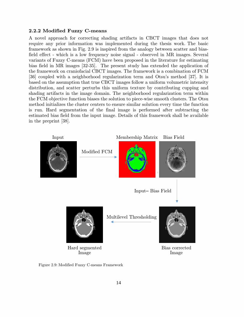
A novel approach for correcting shading artifacts in CBCT images that does not require any prior information was implemented during the thesis work. The basic framework as shown in Fig. 2.9 is inspired from the analogy between scatter and bias-field effect - which is a low frequency noise signal - observed in MR images. Several variants of Fuzzy C-means (FCM) have been proposed in the literature for estimating bias field in MR images [32-35]. The present study has extended the application of the framework on craniofacial CBCT images. The framework is a combination of FCM [36] coupled with a neighborhood regularization term and Otsu's method [37]. It is based on the assumption that true CBCT images follow a uniform volumetric intensity distribution, and scatter perturbs this uniform texture by contributing cupping and shading artifacts in the image domain. The neighborhood regularization term within the FCM objective function biases the solution to piece-wise smooth clusters. The Otsu method initializes the cluster centers to ensure similar solution every time the function is run. Hard segmentation of the final image is performed after subtracting the estimated bias field from the input image. Details of this framework shall be available in the preprint [38].

Multilevel Thresholding

Modified FCM

Input

Input– Bias Field

Bias Field Membership Matrix

Figure 2.9: Modified Fuzzy C-means Framework

Hard segmented Image

Bias corrected Image

14

2.3 Evaluation Metrics

The evaluation metric includes the following examinations:

I. Two Sample T-test The two sample T-test [39] is a statistical test to imply if the means of two groups are reliably different from one another. Mean is a descriptive statistic that describes the result but cannot be generalized beyond that. On the other hand inferential statistics like T-test allows us to make inferences about our predictions beyond the given data.

II. Confusion Matrix

Confusion matrix demonstrates the sensitivity (true positive rate) and specificity (true negative rate) of the results. Sensitivity measures the proportion of actual positives which are correctly identified as such (e.g. the percentage of bone pixels correctly classified as bone pixels). Mathematically,

Sensitivity =number of true positives

number of true positives + number of false negatives

Specificity measures the proportion of negatives which are correctly identified as such (e.g. the percentage of no-bone pixels which are correctly identified as no-bone). Mathematically,

Specificity =number of true negatives

number of true negatives + number of false positives

III. Execution Time

IV. ROI error Several regions in craniofacial CBCT images such as Dorsum Sellae and Clivus are hard to segment due to poor image contrast. Hence, 5 regions of interest (ROIs) were manually defined in CBCT images and classification error within ROI's was calculated.

𝑅𝑅𝑅𝑅𝑅𝑅𝑒𝑒𝑒𝑒𝑒𝑒𝑅𝑅𝑒𝑒𝑖𝑖 =1𝑁𝑁�𝑛𝑛𝑛𝑛𝑛𝑛𝑁𝑁

𝑖𝑖=1

(𝑃𝑃𝑖𝑖𝑖𝑖 − 𝐿𝐿𝑖𝑖𝑖𝑖) ∀ 𝑘𝑘 ∈ {1,2,3,4,5}

where 𝑁𝑁 is the number of test images.

𝑃𝑃𝑖𝑖𝑖𝑖 𝑎𝑎𝑛𝑛𝑎𝑎 𝐿𝐿𝑖𝑖𝑖𝑖 are the predicted and label vectors for the 𝑘𝑘th ROI in the 𝑖𝑖th test image respectively.

𝑛𝑛𝑛𝑛𝑛𝑛 is a function evaluating number of non-zeros.

V. Visual Inspection

The aim of visual inspection is to analyze regions within images that are more susceptible to misclassifications due to different segmentation methods.

(7)

(9)

(8)

15

3. Results

This chapter covers the results generated by the aforementioned methods. All simulations were performed on a desktop computer with Intel Core i7-4790K CPU, 32 GB RAM and NVIDIA GeForce GTX 970 4GB. The training of MLP was performed on the aforementioned CPU and took 6 days to complete. The training of CNN was performed on the aforementioned GPU and took 2 days to complete. In order to maintain result fidelity, none of the 20 test images were exposed to any of the segmentation algorithm during training process for parameter tuning. The results presented below are first time evaluations on test images and no parameter tuning was performed after this. All test images have a fixed size of 512 x 512 x 154.

3.1 Two Sample T-Test

Methods Evaluation Metric

Mean Error %

Standard Deviation %

Execution Time (s)

Thresholding 1.1 0.18 0.9

MFCM 0.8 0.12 64*

MLP 1.2 0.19 92

CNN 0.4 0.07 500 Table 3.1: Mean classification error and execution times over 20 test images. Best scores in every metric are marked in bold. Execution times marked with an * symbolize that the test was performed on CPU. Else, the test was performed on GPU. Table 3.1 shows that CNN based segmentation, results in the minimum classification error and variance among test CBCT images. Yet, at the cost of long execution time. For a T-test, we assume that the null hypothesis states no statistically significant difference between means of two methods. Test result is 1 if it rejects the null hypothesis at the 5% significance level, and 0 otherwise. In case the test result is 1, it is concluded that the group with lower mean error is better. A P-value is the probability of observing the result by chance if the null hypothesis is true. Smaller p-values are preferred. Table 3.2 shows a generalization that in at least 95% of cases, CNN shall outperform other segmentation techniques on CBCT images. MFCM proves to be the second best segmentation algorithm outperforming MLP and multi-level thresholding. MLP and multi-level thresholding show no statistically significant difference among their performance.

16

Method 1 Method 2 Result P-value

CNN Thresholding 1 < 0.001

CNN MFCM 1 < 0.001

CNN MLP 1 < 0.001

MFCM Thresholding 1 < 0.001

MFCM MLP 1 < 0.001

Thresholding MLP 0 0.08 Table 3.2: T-test results for comparing mean errors of different segmentation methods.

3.2 Confusion Matrix

Methods Evaluation Metric

Specificity Sensitivity

Bone Tissue Air Bone Tissue Air

Thresholding 99.9 98.8 99.6 85.3 99.3 99.7

MFCM 99.8 99.3 99.4 91.7 98.5 99.8

MLP 99.1 99.6 99.7 98.1 95.9 99.7

CNN 99.8 99.7 99.4 97.9 98.7 99.8 Table 3.3: Confusion matrix for bone, tissue and air.

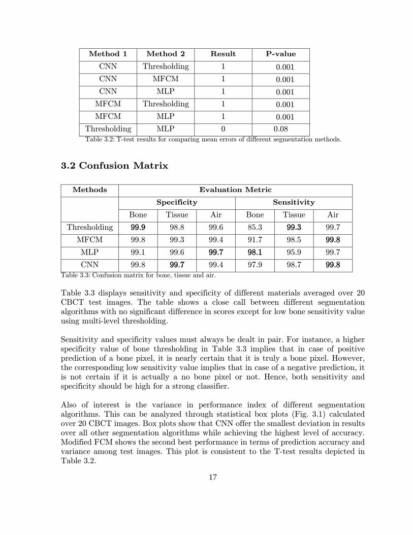
Table 3.3 displays sensitivity and specificity of different materials averaged over 20 CBCT test images. The table shows a close call between different segmentation algorithms with no significant difference in scores except for low bone sensitivity value using multi-level thresholding. Sensitivity and specificity values must always be dealt in pair. For instance, a higher specificity value of bone thresholding in Table 3.3 implies that in case of positive prediction of a bone pixel, it is nearly certain that it is truly a bone pixel. However, the corresponding low sensitivity value implies that in case of a negative prediction, it is not certain if it is actually a no bone pixel or not. Hence, both sensitivity and specificity should be high for a strong classifier. Also of interest is the variance in performance index of different segmentation algorithms. This can be analyzed through statistical box plots (Fig. 3.1) calculated over 20 CBCT images. Box plots show that CNN offer the smallest deviation in results over all other segmentation algorithms while achieving the highest level of accuracy. Modified FCM shows the second best performance in terms of prediction accuracy and variance among test images. This plot is consistent to the T-test results depicted in Table 3.2.

17

Figure 3.1: Box Plots showing statistical distribution of prediction accuracy for different segmentation algorithms evaluated over 20 test images. For each box, the red mark indicates the median, and the bottom and top edges of the box indicate the 25th and 75th percentiles, respectively. The whiskers extend to extreme data points that are not considered as outliers. + Symbol indicates outliers.

Segmentation Method

CNN MFCM MLP Thesh

Cor

rect

Pre

dic

tion

Rat

e %

98.8

99

99.2

99.4

99.6

99.8

BoxPlot for Bone Prediction

Segmentation Method

CNN MFCM MLP Thesh

Cor

rect

Pre

dic

tion

Rat

e %

98.4

98.6

98.8

99

99.2

99.4

99.6

BoxPlot for Tissue Prediction

18

3.3 ROI error

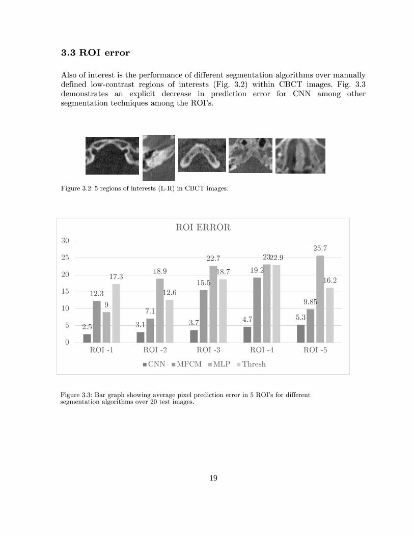
Also of interest is the performance of different segmentation algorithms over manually defined low-contrast regions of interests (Fig. 3.2) within CBCT images. Fig. 3.3 demonstrates an explicit decrease in prediction error for CNN among other segmentation techniques among the ROI's.

Figure 3.2: 5 regions of interests (L-R) in CBCT images.

2.5 3.1 3.7 4.7 5.3

12.3

7.1

15.5

19.2

9.859

18.9

22.7 2325.7

17.3

12.6

18.7

22.9

16.2

0

5

10

15

20

25

30

ROI -1 ROI -2 ROI -3 ROI -4 ROI -5

ROI ERROR

CNN MFCM MLP Thresh

Figure 3.3: Bar graph showing average pixel prediction error in 5 ROI's for different segmentation algorithms over 20 test images.

19

3.4 Visualization Fig. 3.4 provides a visual comparison of different segmentation algorithms. The three

color schemes – black, gray and white – represent air, soft tissue and bone regions respectively. It is observed that CNN provide the most similarity with the ground truth followed by MFCM. It is also shown that multi-level thresholding (F) obscures certain low contrast bone regions around central craniofacial anatomy as discussed in the low sensitivity value in Table 3.3. MFCM (D) outperforms multi-level thresholding because of bias correction which smooths out shading artifacts in the images. MLP (E) demonstrates a slight noisy segmentation. This is due to lack of contextual information captured within the 9 training features.

A. Input Slices

B. Ground Truth

20

C. CNN

D. MFCM

E. MLP

F. Multilevel Thresholding

Figure 3.4: Visual comparison of different segmentation algorithms.

21

4. Discussion

This chapter discusses the results; highlights major challenges involved during the work and suggests improvements.

4.1 Performance

Table 3.1 shows that CNN outperforms other segmentation techniques in term of classification accuracy. However, they also require the highest execution time because of the complex architecture. Table 3.1 also depicts that histogram based thresholding give a good enough classification performance in minimum time. In a strict mathematical sense, the difference in classification performance between CNN and

multi-level thresholding (~0.7%) seems to be fairly low compared to the time and resources needed for CNN implementation. However it must be noted that 0.7% of misclassification in volumetric images of size (512x512x154) implies approximately 300,000 misclassified pixels. These misclassifications are mostly seen around the low-contrast regions of central anatomy (Fig. 3.4 E) and it obscures crucial structural information. This is graphically explained in Fig. 4.1. The plot depicts the number of bone pixels per slice for a test CBCT image. It is apparent that significant bone information is lost via multi-level thresholding around regions inferior to the patient

head top (axial slices 20 to 50) when compared to the dotted red reference line – the ground truth. However, CNN (blue line) shows a considerable match to the ground truth.

Figure 4.1: Bone information per craniofacial CBCT slice in transverse plane. The highest slice No. corresponds to top of the head. 22

Another important contribution of CNN is the stability in their results as shown in Fig. 3.1. Reliability and validity are significant assessment tools of a system. Reliability is the degree to which the system outputs consistent results. Validity is the quality of being factually correct. CNN achieves high reliability and validity by capturing intrinsic noise-free features from images. Hence, the output of CNN is resistant to image artifacts. Shading artifacts are a major source of non-uniform pixel intensities in CBCT images which make multi-level thresholding less reliable and valid in its results. MFCM performs shading correction prior to segmentation which makes the results more reliable and valid compared to multi-level thresholding. A key ingredient behind the success of CNN prediction is the choice of patches centered on edge voxels as explained in section 2.1.1 II. Contrary to random patches extracted from CBCT images, it was observed that the mean segmentation error on test images was reduced by 70% when the CNN was trained using patches around edge voxels. The choice of CNN architecture (order and size of layers) is also a crucial element governing the classification accuracy. The present CNN architecture was determined by iteratively running different combinations of network layers and sizes and comparing the validation scores. However, there is always a room for incorporating more efficient network architectures to improve classification accuracy. Different variants of patch dimensions (Fig. 2.4) were tried during the course work. However, the network performance was optimized for 2D patches only. Further investigation on 3D patches might be of interest in improving network efficiency. An alternative approach is to make use of deep convolutional encoder networks (CEN) [40]. Contrary to our existing patch-based CNN model, CEN has intermediate convolution and deconvolution blocks which extracts features from the entire image rather than patches. Hence, they provide a similar sized mapping of input and output images and eliminate the steps of patch selection and redundant calculations at the overlap of neighboring patches. However, considering the size of CBCT images, a major drawback of CEN is that it would approximately require a 40 times extra processing memory to perform training. A major drawback in CNN performance is the high execution time. This includes time required for creating patches (Fig. 2.4) and then generating output for every patch (Fig. 2.5). Possible solutions to this limitation include:

i. Using a stronger GPU in terms of size or using multiple GPUs. ii. Generate test patches on GPU rather than CPU. iii. Using advanced CNN libraries such as Caffe [41] with cuDNN

acceleration [42].

23

4.2 Limitations

Since the ultimate aim of the segmentation step is to assist in the iterative reconstruction of CBCT images (section A.5.2), a further study targeting the impact of different segmentation techniques on CBCT projection generation is required. This specific study shall draw the boundary conditions of our confusion matrix. For instance, the study shall highlight how lower or higher sensitivity/specificity values of bone, tissue or air voxels impact the CBCT projection generation which in turn effects 3D image reconstruction. A notable limitation of this work lies in the limited number of segmentation algorithms tested on CBCT images. A further study addressing the performance of new segmentation techniques such as level set, region growing, graph partitioning etc. is essential to generalize the performance of CNN over other segmentation algorithms. Also of interest is to attempt improvements in the existing tested methods, for instance, improved features extraction for MLP etc.

Since Leksell Gamma Knife Icon was introduced in May 2015, a major challenge in implementing a deep framework was the unavailability of expert segmented real CBCT images for training. Hence, it is worth mentioning that no real CBCT data was used during the thesis work. Synthetic CBCT images - generated from stereotactic CT

dataset - were used for training and testing (Fig 2.1 – I) as explained in section 2.1.1. However, the use of real CBCT images in future is important to certify the authenticity of the results on clinical level. Another question to be addressed is that the present study is based on a strong assumption that CT images are less sensitive to noise artifacts compared to CBCT images which make CT segmentation using thresholding operation very accurate. Following this assumption, segmented CT images were used as the ground truth for CNN training. However, this assumption is not exactly true. For instance, conventional CT is more sensitive to beam hardening artifacts primarily due to a higher energy spectrum [43]. During the data preparation process as explained in Fig. 2.1 (steps A-E), metallic screws fastening the stereotactic frame to the skull could not be entirely removed. These screws penetrate through the skin (see Fig. 2.2) and cause streaking artifacts. Severe beam hardening was also apparent in the maxillofacial region in some CT images. This significantly deteriorates the quality of ground truth obtained

through thresholding – Fig 4.2. The availability of expert segmented CBCT images in future is likely to overcome this problem. Another possible fix is to make use of advanced tomogram segmentation algorithms that determine thresholds from the projections rather than reconstructed volumes [44, 45].

24

An additional issue to be thought of is that the entire CT data used to generate the CBCT images and ground truth for training and testing was obtained from a single clinical center (anonymous). This means that this data is likely to have inherited some unwanted traits specific to scanner deformations, user protocols etc. Hence, there is a possibility that the trained CNN model might not work with a similar performance index at another clinical site. However, since training architecture is implemented, it is advisable to tune the CNN parameters using data from new sites before practical implementation. Medical data handling is a sensitive exercise involving high level of integrity and probity. CT data from Elekta was provided in DICOM format which groups patient, scanner, protocol and image information in one file. More on DICOM can be found in [46]. Respecting patient's privacy and confidentiality; common tags that describe patient identity such as name, age, sex, ethnic group, occupation, examination date, hospital ID etc. were obscured. Only image information was used as Matlab (.mat) or Python (.py) files for this work. However, since craniofacial anatomy differs slightly among different age groups, sex and geographical locations; it might be of interest in future to make use of this information from DICOM files as separate features in training deep networks. However, it is essential to seek legal consent from the data provider before using this information.

Figure 4.2: An illustration of beam hardening in CT images (left column) deteriorating the ground truth (right column) due to dental anatomy (top row) and metallic stereotactic frame screws (bottom row). Dotted rectangles demonstrate the presence of artifacts.

25

5. Conclusion

Semantic segmentation of Cone Beam CT images was performed using conventional image processing methods, feature-based machine learning technique and feature-independent deep learning framework. The objective of the work was to investigate whether deep learning based CNN surpass the conventional image processing and ML methods in segmenting noisy CBCT images. It was hypothesized that CNN will outperform other algorithms given the aforementioned evaluation metric. Apart from execution time, CNN's have outperformed other segmentation algorithms throughout the evaluation metric. Since execution speed is important for real-time 3D image reconstruction in CBCT, further efforts to speed up CNN execution are required.

26

Appendix A: Background and Literature Review

If the great German Physicist - W. Röntgen - were to return today, what would probably impress him the most from medical evolution? We might shortlist three achievements: resourcefulness of our electronic health record systems in providing secure patient information anywhere and anytime; the vast range and specificity of drugs in our pharmacies; and our ability to look into every inch of human body through

imaging and scoping techniques. Nearly every clinic that Röntgen would encounter would have a busy imaging facility running medical diagnosis or treatment planning, and much of the success behind this achievement can be attributed to his own

discovery of what he called ‘unknown radiations’ or X-radiations. It happened by

chance – as so many things in science do – and marked the beginning of a glittering

career and fame for Röntgen as Father of Diagnostic Radiology that revolutionized the field of medical imaging.

A.1 Computed Tomography

Within months after the discovery of X-radiations in 1895, X-ray images found their

place in clinical environments [47]. In 1917, an Austrian Mathematician – Johan Radon

– showed that any function can be estimated from an infinite number of its projections [48]. However, oblivious to the Radon theorem, an English engineer G. Hounsfield and South African physicist Allan Cormack invented the Computed Tomography (CT) in 1972 [49] inaugurating the era of Digital Medical Imaging. Since then, there has been an explosion of research activities for refining CT technology primarily focusing on better tissue contrast and spatial resolution for medical diagnosis with the constraints of minimum radiation dosage to patients and reduced reconstruction times [50]. Modern third generation CT scanners consist of an X-ray source in a fan geometry that penetrates through the object or patient being scanned, covering a slice section of it. The X-rays are attenuated when penetrating through the object and the local absorption is measured by the detector array. In order to capture a 3D representation, the object is irradiated by rotating the X-ray source and the detector around the object. The local absorptions or projections captured by the detector under different projection angles are used to reconstruct 2D axial slices of the object. Conventional CT generates a 2D slice at every rotation. CT becomes a 3D imaging modality when consecutive slices are arranged as axial stacks. Two broad categories of reconstruction algorithms include direct and iterative methods. Filtered Back Projection (FBP) algorithm is a common example of a direct reconstruction method based on the Radon Transform [51]. The standard FBP algorithm has several fundamental assumptions on scanner geometry and is basically a compromise between image noise and reconstruction speed. With the advent of high speed parallel GPU computations, iterative reconstruction algorithms have attracted huge interest in medical image reconstruction. The field of iterative 3D reconstruction has since been readily evolving; giving rise to a seemingly never ceasing flow of new algorithms [52, 53].

27

Figure A.1: An illustrative operational comparison of conventional fan beam and CBCT systems.

A.2 Cone Beam Computed Tomography

In 1984, Feldkamp, David and Kress (FDK) provided an extension to the FBP method by formulating a 3D reconstruction algorithm using a convolution back projection formula on a set of 2D projections acquired along a circular trajectory [1]. This reconstruction algorithm coupled with the development of continuous exposure x-ray tubes and compact high-quality 2D detector arrays led to the production of Cone Beam CT that expanded the role of X-ray imaging from diagnosis to image guidance in operative and surgical procedures. CBCT is a recent imaging modality. The name cone-beam CT was coined to illustrate the cone shaped divergence of the x-ray beam from the source to detector. It consists of a flat detector that captures 2D projections (rather than slices) of the object at each angular step. The projections are used to estimate a 3D volume of the object being scanned. CBCT mounted on a C-arm is another advancement in Radiology. This configuration provides volumetric imaging capabilities within interventional suites. Historically, medical domains such as interventional radiology and implant industry had been using 2D radiographic imaging techniques like digital subtraction angiography to visualize, manipulate and intervene on 3D structures [3]. C-arm CBCT systems may also be physically attached to a therapeutic device such as proton therapy and linear accelerators [54]. This intervention inaugurated the era of Image Guided Radiotherapy (IGRT) where frequent imaging during the course of treatment helps in improving the precision and accuracy of the radiation source. Recently, Elekta utilized the C-arm CBCT functionalities by physically attaching it to Gamma Knife to determine patient position prior to radiosurgery [55]. In the present frame of work, we are interested in the latter application of CBCT.

28

CBCT has several advantages over traditional CT which make it suitable for point-of-care applications. It offers a small footprint, low cost and an adaptable geometry that qualifies it to be physically attached to a surgical device like Gamma Knife. It also offers a better isotropic spatial resolution. In conventional CT, the voxels are anisotropic rectangular cubes with plane dimensions as small as 0.6mm and voxel depth determined by the axial slice thickness - usually in the order of 1-2mm. The volumetric dataset of CBCT comprises of isotropic cubic voxels that determine the resolution of the image which range from 0.4mm to 0.076mm [56]. Last but not least, CBCT has proven to offer lower radiation dosage compared to conventional CT systems [3, 21]. The price paid for all the above mentioned advantages is poor image contrast and significantly higher noise artifacts compared to conventional CT.

A.3 CBCT System at Elekta

Lars Leksell – a Swedish Physician – developed the concept of Radiosurgery in 1951 [57]. Radiosurgery is a surgical treatment targeting and destroying tumor cells with an ionizing radiation source. The word stereotactic refers to a 3D coordinate system used to locate the target site within the cranial region. Lars, later invented the Gamma Knife in 1967 and founded Elekta in 1972. Gamma Knife stereotactic radiosurgery by Elekta has since been one of the top treatment choice for brain tumors and functional disorders around the globe. In the Gamma-Knife, Gamma-rays emitted from multiple radioactive 60Co sources arranged in a hemi-spherical array are focused on a single point of the brain creating a high spherical dose to destroy tumor cells. The target site (tumor) of the patient is at first located using Magnetic Resonance (MR) scan in a separate room. This is termed as the planning image. The patient is then transferred for a surgical session to Gamma Knife. The planning images are then mapped onto stereotactic coordinates defined for Gamma Knife. This mapping involves annotations on planning images by a physician using the Leksell Frame System [4]. The Leksell Frame has certain

drawbacks. The metallic frame fixation to the patient’s head is an invasive procedure leading to patient discomfort and enhanced treatment time. Second, Dose

Fractionation – which is a common protocol in radiation oncology [58] - is cumbersome to perform using the frame based system. The-state-of-the-art, Leksell Gamma Knife Icon introduced an image guidance system based on CBCT to enable fractionated, frameless and time efficient surgeries while maintaining similar precision levels as is achieved by the Leksell Frame. A C-arm CBCT system attached to Gamma Knife provides the stereotactic reference prior to surgical session. Planning MR images are then co-registered to stereotactic CBCT images automatically for determining patient position relative to Gamma Knife coordinates at the time of surgery.

29

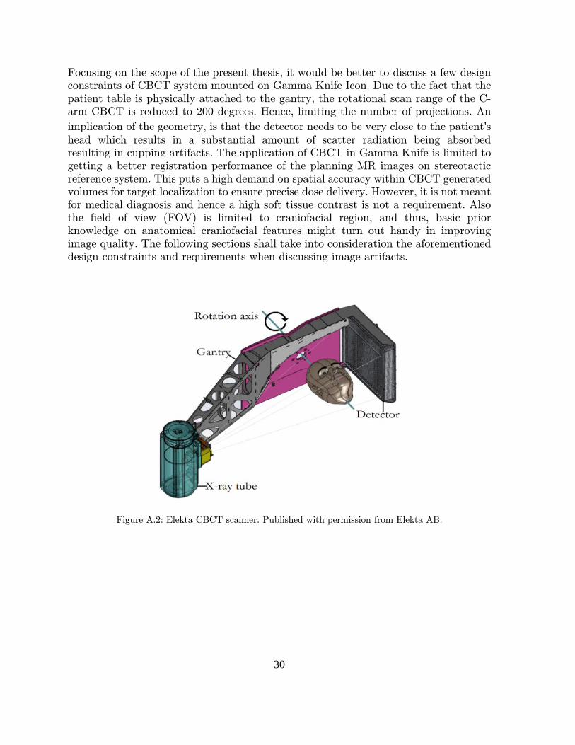
Focusing on the scope of the present thesis, it would be better to discuss a few design constraints of CBCT system mounted on Gamma Knife Icon. Due to the fact that the patient table is physically attached to the gantry, the rotational scan range of the C-arm CBCT is reduced to 200 degrees. Hence, limiting the number of projections. An

implication of the geometry, is that the detector needs to be very close to the patient’s head which results in a substantial amount of scatter radiation being absorbed resulting in cupping artifacts. The application of CBCT in Gamma Knife is limited to getting a better registration performance of the planning MR images on stereotactic reference system. This puts a high demand on spatial accuracy within CBCT generated volumes for target localization to ensure precise dose delivery. However, it is not meant for medical diagnosis and hence a high soft tissue contrast is not a requirement. Also the field of view (FOV) is limited to craniofacial region, and thus, basic prior knowledge on anatomical craniofacial features might turn out handy in improving image quality. The following sections shall take into consideration the aforementioned design constraints and requirements when discussing image artifacts.

Figure A.2: Elekta CBCT scanner. Published with permission from Elekta AB.

30

A.4 CBCT Artifacts

Artifacts are image errors that deteriorate image quality. They can be broadly classified into three categories. (i) Physics based artifacts; that result due to our assumptions, simplifications and modelling limitations of the physical processes involved in the acquisition and reconstruction of CBCT data [51]. (ii) Scanner based artifacts; that occur due to imperfections in scanning geometry, defective detector elements etc. (iii) Patient based artifacts; that occur due to patient movements. Understanding the source of artifact is crucial for applying correction measures. The present thesis focuses on physics based artifacts.

A.4.1 Scatter

Scatter is a big concern in CBCT imaging. Scatter radiation is caused by photons that after interaction with matter, get diffracted from their original path and add to the measured intensities of primary photons. Unlike the fan beam geometry in conventional CT where most of the scatter radiation gets dispersed away from the detector, scatter radiation has a large possibility of interacting with the 2D detector in CBCT. Streak and shading artifacts commonly occur due to scatter radiations [43].

A.4.2 Beam Hardening

The FBP method assumes that the X-radiation is monochromatic – all photons have the same energy [51]. This is assumed to calculate a homogenous attenuation coefficient (dependent only on beam path length) when X-rays pass through an object being radiographed. In practice X-ray beam is polychromatic and from a physical perspective, attenuation coefficients are non-linearly dependent on the density of material being radiographed. Denser the object, the more radiation it absorbs. The low energy rays get more absorbed when passing through the object than high energetic rays within the polychromatic spectrum. The beam reaching the detector has high energy (harder) X-ray beams compared to the emitted source. This phenomenon is termed as beam hardening [59]. Metals and bony structures are a major cause of this artifact. Since this artifact is produced due to the monochromatic assumption in

the reconstruction algorithm – which in turn is same for both CT and CBCT – beam hardening is present in both tomography techniques. CBCT, however is less sensitive to beam hardening due to its low energy spectrum.

A.4.3 Cone-beam artifact

Cone-beam artifact is commonly visible in the periphery of scan volumes. As the X-ray source rotates around the patient in a horizontal arc, the amount of data recorded at the peripheral pixels of the detector is less compared to central detector pixels. Cone beam artifact is proportional to the cone beam angle and smears out flat planar (xy-plane) structures in the z-direction [51].

31

A: Scatter noise significantly disturbing tissue contrast and homogeneity in CBCT scan (right) compared to CT scan (left)

B: Beam Hardening artifact in CT (left) and CBCT (right) showing dark streaks along the lines of greatest attenuation and bright streaks in the other direction.

C: Cone Beam artifact visible on the top region of the head in CBCT scan (right).

Figure A.3: The above illustrations show basic artifacts in CBCT images. Dotted Rectangles demonstrate the presence of artifacts. Published with permission from Elekta AB.

32

A.5 CBCT Denoising Methods

Since the introduction of CBCT in 2001 [60], numerous algorithms have been proposed to tackle its noise artifacts. These correction algorithms can be broadly grouped into two categories.

A.5.1 Hardware approaches

Hardware approaches are basically pre-acquisition methods that are specific for a particular artifact. For instance, in case of scatter artifacts, hardware approaches tend to use air-gaps [61] or anti-scatter grids [62] to prevent scatter photons from reaching the CBCT detector. Similarly, beam filtration using bow-tie filters is an example of hardware correction for beam hardening artifact where an attenuation plate is placed between the source and object to shift the x-ray spectrum towards high-energy end [63]. There are three major drawbacks of hardware approaches. First, they tend to reduce the number of primary photons from reaching the detector, thus decreasing signal to noise ratio (SNR). As a result, higher patient dose is delivered to maintain image contrast. Second, they are specialized for single artifact correction and do not account for image correction in general. Third, they require an add-on device that complicates the hardware on site.

A.5.2 Software approaches

These methods can be divided into three categories:

I. Pre-acquisition correction These methods tend to adjust the gain variations of detector pixels prior to acquisition phase. They make use of beam filters to calculate the ratio between ideal and measured pixel values - Gain Correction Factor - for every pixel. They have shown promising results in eliminating ring artifacts [64]. However, they do not account for other common physics based artifacts such as scatter noise.

II. Post reconstruction correction Post reconstruction techniques are general methods that tend to eliminate shading artifacts from reconstructed images. They include image transformation algorithms coupled with prior information - usually CT images - to minimize the difference between the reconstructed CBCT image and CT image of the same patient [65-68]. The common idea is to build a mathematical fitting model that minimizes a distance metric between the CT and CBCT pixel values. This approach is highly dependent on prior information since it requires exact CT - CBCT image pairs to estimate the polynomial function. In radiotherapy applications, the CT information is gathered from planning images captured by conventional fan beam CT. However, it is desirable to replace CT planning images with MR images due to higher tissue contrast and no radiation exposure [69]. In the context of radiosurgery applications such as Gamma Knife, planning images are often never acquired through CT scans. Rather, MRI scans are used. This impedes the general use of polynomial fitting approach for shading correction in CBCT images.

33

III. Correction within reconstruction These include analytical and iterative reconstruction techniques that tend to include mathematical-physical models for estimating scan objects, scatter contribution in projections, noise levels and system nonlinearities in a deterministic and statistical manner respectively. Iterative reconstruction algorithms - due to a more realistic

approach – are seen as a bellwether in the reconstruction domain. They have demonstrated improved noise suppression while maintaining image features in emission

tomography [70, 71] and computed tomography [72, 73]. FDK – an analytical reconstruction algorithm - is currently used in Gamma Knife Icon and Elekta is investing in significant research to alleviate the artifact problems via state-of-the-art iterative methods. Iterative approaches tend to minimize a cost function iteratively which is constructed based on noise characteristics of the measured data. Accurate noise modelling is essential for statistical iterative algorithms. And hence there has been a series of research activities giving birth to specialized techniques for targeting particular artifacts in the measured data. These include (i) Monte Carlo simulations for modelling scatter noise by tracing the photon path from source to detector and performing corrections in the projection domain [74]. This method is considered to be the most accurate approach for scatter estimation but is computationally burdensome.(ii) Analytical kernel methods using scatter convolution kernels to approximate scatter model [75]. These models offer a balance between computational burden and accuracy. Fig. A.4 briefly explain the overall picture of CBCT image creation. Fig. A.5 and A.6 include the classical steps in an iterative reconstruction algorithm and a typical example of how an analytical scatter estimation model works respectively. Either way, segmentation plays a small but crucial part in both algorithms. The current scope of work is limited to a better segmentation method to be run within the iterative reconstruction loop to assinst image denoising. In order to have a real-time 3D reconstruction, the segmentation step needs to be fast and robust.

Figure A.4: Basic steps in CBCT image creation. The present thesis work is focused within the volume reconstruction block.

Capture 2D X-ray

projections

Pre-processing

Volume Reconstruc

-tion

Post-processing

Visualiza-tion

34

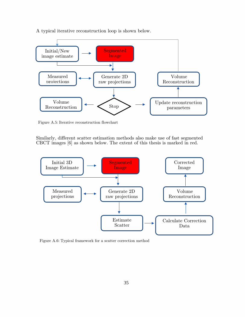
A typical iterative reconstruction loop is shown below. Similarly, different scatter estimation methods also make use of fast segmented CBCT images [6] as shown below. The extent of this thesis is marked in red.

Generate 2D raw projections

Segmented Image

Initial/New image estimate

Measured projections

Volume Reconstruction

Stop Volume

Reconstruction Update reconstruction

parameters

Generate 2D raw projections

Segmented Image

Initial 3D Image Estimate

Measured projections

Volume Reconstruction

Estimate Scatter

Calculate Correction Data

Corrected Image

Figure A.5: Iterative reconstruction flowchart

Figure A.6: Typical framework for a scatter correction method

35

A.6 Segmentation

Automated image segmentation is a fundamental problem in medical image analysis. The applications include contouring organs, lesion (tumor) detection, dose calculations, noise reduction etc. In the present work scope, the aim of the segmentation is to divide the image into homogenous meaningful regions. It is basically a classification problem where every voxel belongs to a particular class. This form of segmentation is also referred as semantic segmentation. There are three broad categories of segmentation methods. (i) Segmentation based on local information. These algorithms tend to work from an image processing viewpoint based morphological and thresholding algorithms [76, 77]. These methods are sensitive to image noise and non-uniform object textures among others [78]. (ii) Segmentation based on a priori information. These are high-level methods that make use of prior information of the expected volume and adapt it to the actual volume. They include deformable models and atlas-based segmentations [10]. These methods are often combined together for segmentation purposes [11, 12]. However, there are two main problems with these methods. First, they require a rich database for constructing atlases. Second, these methods require a smooth transformation between expected and actual volumes. Tumors and other pathological conditions may disrupt this transformation. (iii) Machine Learning (ML) based segmentation techniques have recently shown huge success in medical image analysis with focus on MRI and CT images [14]. They tend to segment lesions or tumor sites within scan volumes and even anatomically segment the entire scan volume into homogenous regions [79]. These methods make use of supervised learning principles where a set of training data and corresponding true labels are fed into a network for training under a certain ML algorithm. The network model is trained to identify the best fitting relationship between the inputs and outputs in a generalized manner. More information on ML algorithms can be found in [15]. A key ingredient behind the success of ML based segmentation methods is the way how the input data is represented. Better image representation often leads to a better analysis. We call it Feature Engineering and Selection and it has been an active research topic in the past decade [80]. Harr wavelet [81] and histogram of oriented gradients [82] are some common examples of feature engineering used for medical image analysis. A major drawback of these so called hand-crafted features is that they are unable to extract salient information from the data. As a result their performance varies from dataset to dataset. Contrary to such traditional classification methods that are dependent on feature engineering, deep learning networks directly extract hierarchical features that are adapted to the dataset [16]. Deep learning based methods for medical image segmentation have shown to outperform the traditional feature based methods on MR images [17, 18]. However, unlike MRI segmentation, these methods have yet not been tried for semantic CBCT segmentation. There are two main reasons for it. First, well labelled CBCT data is not openly available for training deep architectures. Second, CBCT data, unlike MRI, is extremely noisy which poses problem for segmentation.

36

Appendix B: Image Processing and Segmentation

B.1 Image Filtering

Image filtering is a neighborhood operation used to enhance image quality by emphasizing on certain features and depreciating others. Noise is invariably present in digital images. Noise in CBCT images can be broadly grouped into two categories:

1. Signal independent noise: This includes electrical and additive noise. Electrical noise may originate due to several factors involved in the image acquisition process like digital discretization, sensor noise etc.

2. Signal dependent noise: Quantum noise is the photon-count noise that occurs due to uncertainty in the amount of X-ray photons being absorbed by the detector after passing through an object. Quantum noise can be modelled by Poisson's distribution and is often taken care of in the iterative reconstruction process [43].

These noise sources introduce irregularities in the projection images which cause problems in the reconstructed image. However, for simplicity, we shall consider both these noise as additive (signal independent). Hence, we assume that noise is modelled as Additive White Gaussian Noise (AWGN).

𝑉𝑉𝑖𝑖 = 𝑈𝑈𝑖𝑖 + 𝑁𝑁𝑖𝑖 ∀ 𝑖𝑖 ∈ 𝑅𝑅 𝑤𝑤ℎ𝑒𝑒𝑒𝑒𝑒𝑒 𝑖𝑖 is the pixel belonging to the image set of pixels 𝑅𝑅. 𝑈𝑈 is the assumed true noiseless image. 𝑉𝑉 is the noisy image. 𝑁𝑁 is the noise distribution with mean 0 and standard deviation 1.

B.1.1 Gaussian Filtering

Gaussian filtering is a linear spatial operation that convolves the input volume with a Gaussian function kernel [83]. It performs smoothing of the image by replacing every pixel value by the average of its neighbors defined by the kernel window. In the Fourier domain, it gets rid of the high frequency signal which is assumed to be mostly noise. However, high frequency image features such as edges and corners are also lost in the operation.

B.1.2 Non-Local Means Filtering (NLM)

Unlike the Gaussian filtering that denoises images by averaging pixels in the neighborhood kernel, NLM filtering averages similar pixels in the image. The main difference lies in the concept of neighborhood used by the two methods. The neighborhood of a pixel A in NLM filtering includes a set of pixels B such that the window around B pixels (usually Gaussian) is similar to the window around A. Every pixel in B carries a similarity weighting factor that influences the averaging operation. This idea was first proposed by [84] and [85] motivated the use of NLM filtering for denoising CBCT projections.

(10)

37

B.2 Automatic Thresholding

This is a histogram based hard segmentation method where pixels are quantized based on a fixed threshold. Valleys in the image histograms determine the threshold points as shown in Fig. B.1. Otsu's method was originally developed to identify a single threshold value to separate the fore and background images [37]. However, in the present work a modified version of the Otsu's method is used to determine multi-thresholds allowing multi-class segmentation [86].

Figure B.1: Automatic Thresholding

B.3 K-means

K-means is an image clustering algorithm where pixels are grouped together based on a similarity matrix [87]. In case of grayscale CBCT images, Euclidian distances between the grayscale values of pixels is the simplest approach for segmenting the image. The algorithm is given below:

a. Randomly choose K initial cluster centers. b. Assign each pixel to the closest cluster c. Update cluster centers as the average of pixels assigned to each cluster. d. Continue until there is no change in center values of the clusters.

A major limitation with the algorithm is that it does not take spatial coherence into account.

B.4 Fuzzy C-means

Fuzzy C-means algorithm is very similar to K-means, except for step b in the latter algorithm. Rather than hard assigning each pixel to its closest center, Fuzzy C-means creates a partition matrix that stores a membership vector for every pixel defining the degree to which that pixel belongs to all the K clusters [36]. Fuzzy C-means also does not take into account spatial coherence.

38

B.5 Mean Shift

Mean shift is also a clustering based segmentation method that includes spatial information (x,y,z) and grayscale values of the pixels [88]. Mean shift considers this four dimensional input vector as an empirical probability density function. This means that peaks of the density function imply true clusters or segments in the image. These peaks are found iteratively using a gradient ascent function. The basic algorithm works as follows

a. Determine a window (often called as bandwidth) around each image pixel b. Calculate the data mean within the bandwidth c. Shift the window to the new mean and continue until convergence.

A major drawback of mean shift is that we do not get control over number of clusters or segments. It is also computationally demanding.

B.6 Multilayer Perceptron

Artificial Neural Networks (ANN) are machine learning techniques inspired and loosely based on biological neural networks. Multilayer Perceptron (MLP) is a type of supervised ANN which was developed to overcome the limitation of a linear perceptron that only classifies linearly separable data. MLP consists of one or more feed-forward hidden layers that rest between the input and output layers and are used to model non-linearity in the feature space. Each layer in a MLP is fully connected to the next one via weights: an input layer that receives external inputs, hidden layers and an output layer which generates the classification results (Fig. B.2). Except for the neurons in the input layer, every neuron is a computational element with a summation processor and a nonlinear activation function. Rumelhart discovered a way to train MLP using backpropagation of error in which weights between nodes are trained so that the error (difference between output and target value) goes downhill [89]. This is a gradient descent algorithm in which the weights are adjusted to change the value of E (error) in the direction of negative gradient to find a global minima on the error surface.

Figure B.2: Multilayer Perceptron

39

B.7 Convolutional Neural Networks

Convolutional Neural Networks (CNN) belong to the group feed-forward artificial neural networks where the connectivity pattern between different layers is inspired by the connectivity in the animal visual cortex. CNN offer a hierarchical method of data representation as shown in Fig. B.3. For instance, in language processing applications features may be sorted into letters, words, phrases, sentences and finally a story.

The animal visual cortex - first explored by Hubel [90] - is a complex processing system that extracts strong spatial correlations within images via a mosaic cellular arrangement covering the entire visual field. Every cell in the visual cortex is sensitive

only to a small region of the visual field – often known as its receptive field. Efforts to emulate the architecture of animal visual cortex led to the introduction of convolutional neural network that rests on the principles of local connectivity and extensive weight-sharing [19]. This allows handling high-dimensional data such as images and videos without the need of big networks (number of nodes) and longer processing times.

B.7.1 Computational Blocks

Conventionally, CNN's are built from five fundamental blocks.

I. Convolution Block This block takes in a randomly initialized filter bank of arbitrary size and performs 2D or 3D convolution operation on the input image. Simply stating, convolution means applying a filter over an image at all possible offsets. The convolution of a 2D image

𝑓𝑓(𝑥𝑥, 𝑦𝑦) with a filter ℎ of size (2𝑁𝑁 + 1) x (2𝑀𝑀 + 1) is given as:

𝑎𝑎(𝑥𝑥, 𝑦𝑦) = (ℎ ∗ 𝑓𝑓)(𝑥𝑥,𝑦𝑦) = � � ℎ(𝑎𝑎,𝑛𝑛)𝑓𝑓(𝑥𝑥 − 𝑎𝑎,𝑦𝑦 − 𝑛𝑛)𝑁𝑁

𝑛𝑛=−𝑁𝑁

𝑀𝑀

𝑚𝑚=−𝑀𝑀

Intuitively, the filters are analogous to visual cells in the animal cortex. The size of the filter corresponds to the receptive field of a visual cell. At one instant, the filter is only wired to a sub-region of the input image equivalent to the size of the filter - local connectivity. As the filter is swiped through the image along horizontal and vertical directions during convolution, dot product of the filter with its corresponding receptive

(11)

Image in Low Level features (pixel

intensitiesetc.)

Mid-Level features (edges,

motif etc.)

High Level

features (objects

etc.)

Trainable Classifier

Figure B.3: Features in deep learning in context of images.

40

field on the input image is calculated. This operation highlights the presence of a particular feature within the image at any spatial location. Each filter has same weights - weight sharing - and bias values at every offset and is termed as a feature map. The number of filters correspond to the number of features in the convolution layer and this value is chosen arbitrarily.

II. Spatial Pooling Block This block performs a non-linear down-sampling of the input image. It takes a window size as an input and swipes it along the image in both directions and outputs the maximum or mean value at every offset. Hence, for an input image of size (32x32) and a pool window of size (2x2), the output would be (16x16). This block has two main advantages. First, it reduces computational burden by down sampling the input image. This reduces the dimensionality of the input image, thus avoiding overfitting. Second, it provides a sort of translational invariance in the network, thus adding robustness to the solution.

III. Non-Linearity Block This block is essential to stack multiple layers in the network. Different non-linearity functions also termed as activation functions can be used. Most common are Rectified Linear Unit (ReLU) and Sigmoid. The former transforms all negative values to 0 and the latter computes the sigmoid.

𝑦𝑦 = max {0, 𝑥𝑥 } 𝑅𝑅𝑒𝑒𝐿𝐿𝑈𝑈

𝑦𝑦 = 𝜎𝜎(𝑥𝑥 ) =1

(1 + 𝑒𝑒−𝑥𝑥 ) 𝑆𝑆𝑖𝑖𝑎𝑎𝑎𝑎𝑅𝑅𝑖𝑖𝑎𝑎

IV. Fully Connected Block Nodes in fully connected block have full connections to every node in the previous and next layer. This is similar to MLP discussed in Appendix B.6. This block captures position-dependent information and more global patterns.

V. Softmax Block The softmax operator outputs posterior probabilities for a categorical label. These probabilities lie within 0 - 1 range and sum to 1. The softmax operator is given as

𝑦𝑦 =𝑒𝑒𝑥𝑥

∑ 𝑒𝑒𝑥𝑥𝐷𝐷𝑡𝑡=1

Other important computational blocks include De-convolution, Drop Out, Normalization, Log Loss etc. and details can be found in Matconvnet3 [26].

3 Technical manual available at http://www.vlfeat.org/matconvnet/matconvnet-manual.pdf

(12)

(13)

(14)

41

References

1. Feldkamp, L.A., L.C. Davis, and J.W. Kress, Practical cone-beam algorithm. Journal of the Optical Society of America A, 1984. 1(6): p. 612-619.

2. Jaffray, D.A. and J.H. Siewerdsen, Cone-beam computed tomography with a flat-panel imager: initial performance characterization. Med Phys, 2000. 27(6): p. 1311-23.

3. Orth, R.C., M.J. Wallace, and M.D. Kuo, C-arm cone-beam CT: general principles and technical considerations for use in interventional radiology. J Vasc Interv Radiol, 2008. 19(6): p. 814-20.

4. Maciunas, R.J., R.L. Galloway Jr, and J.W. Latimer, The application accuracy of stereotactic frames. Neurosurgery, 1994. 35(4): p. 682-695.

5. Zhao, W., et al., A model-based scatter artifacts correction for cone beam CT. Medical physics, 2016. 43(4): p. 1736-1753.

6. Zhao, W., et al. A patient-specific scatter artifacts correction method. in SPIE Medical Imaging. 2014. International Society for Optics and Photonics.

7. Bai, Y., et al., Iterative CBCT Scatter Shading Correction Without Prior Information. Medical Physics, 2016. 43(6): p. 3345-3345.

8. Pengwei Wu, T.M., Shutao Gong, Jing Wang, Ke Sheng, Yaoqin Xie, Tianye Niu, Shading correction assisted iterative conebeam CT reconstruction, in The 4th International Conference on Image Formation in X-Ray Computed Tomography, C. meeting, Editor. 2016: Bamberg, Germany. p. 391-394.

9. Wu, P., et al., Iterative CT shading correction with no prior information. Phys Med Biol, 2015. 60(21): p. 8437-55.

10. Sharma, N. and L.M. Aggarwal, Automated medical image segmentation techniques. J Med Phys, 2010. 35(1): p. 3-14.

11. Ciofolo, C. and C. Barillot, Atlas-based segmentation of 3D cerebral structures with competitive level sets and fuzzy control. Medical Image Analysis, 2009. 13(3): p. 456-470.

12. Ghadimi, S., et al., Segmentation of scalp and skull in neonatal MR images using probabilistic atlas and level set method. Conf Proc IEEE Eng Med Biol Soc, 2008. 2008: p. 3060-3.

13. Ledig, C., et al., Robust whole-brain segmentation: Application to traumatic brain injury. Medical Image Analysis. 21(1): p. 40-58.

14. Luping Zhou LW, Q.W., Yinghuan Sh., Machine Learning in Medical Imaging. 2015 ed. 6th International Workshop, MLMI. 2015: Springer International Publishing.

15. Marsland, S., Machine Learning - An Algorithmic Perspective. Machine Learning and Pattern Recognition Series, ed. C.a. Hall/CRC. 2009: Taylor and Francis Group.

16. Deng, L. and D. Yu, Deep Learning: Methods and Applications. 2014: Now Publishers.

17. Brosch, T., et al., Deep Convolutional Encoder Networks for Multiple Sclerosis Lesion Segmentation, in Medical Image Computing and Computer-Assisted Intervention – MICCAI 2015: 18th International Conference, Munich, Germany, October 5-9, 2015, Proceedings, Part III, N. Navab, et al., Editors. 2015, Springer International Publishing: Cham. p. 3-11.

18. Liao, S., et al., Representation learning: a unified deep learning framework for automatic prostate MR segmentation. Med Image Comput Comput Assist Interv, 2013. 16(Pt 2): p. 254-61.

19. Krizhevsky, A., I. Sutskever, and G.E. Hinton. Imagenet classification with deep convolutional neural networks. in Advances in neural information processing systems. 2012.

20. Brosch, T., et al., Deep 3D Convolutional Encoder Networks with Shortcuts for Multiscale Feature Integration Applied to Multiple Sclerosis Lesion Segmentation. IEEE Trans Med Imaging, 2016.

42

21. Nagatani, Y., et al., Ultra-low-dose computed tomography system with a flat panel detector: assessment of radiation dose reduction and spatial and low contrast resolution. Radiat Med, 2008. 26(10): p. 627-35.

22. Ruhrnschopf, E.P. and K. Klingenbeck, A general framework and review of scatter correction methods in x-ray cone-beam computerized tomography. Part 1: Scatter compensation approaches. Med Phys, 2011. 38(7): p. 4296-311.

23. Huang, D.-Y. and C.-H. Wang, Optimal multi-level thresholding using a two-stage Otsu optimization approach. Pattern Recognition Letters, 2009. 30(3): p. 275-284.

24. Kubat, M. and S. Matwin. Addressing the curse of imbalanced training sets: one-sided selection. in ICML. 1997. Nashville, USA.

25. Canny, J., A Computational Approach to Edge Detection. IEEE Transactions on Pattern Analysis and Machine Intelligence, 1986. PAMI-8(6): p. 679-698.

26. Lenc, A.V.a.K., MatConvNet -- Convolutional Neural Networks for MATLAB. Proceeding of the {ACM} Int. Conf. on Multimedia. 2015.

27. Geman, S., E. Bienenstock, and R. Doursat, Neural networks and the bias/variance dilemma. Neural computation, 1992. 4(1): p. 1-58.

28. Nickolls, J., et al., Scalable parallel programming with CUDA. Queue, 2008. 6(2): p. 40-53.

29. Cortes, C. and V. Vapnik, Support-vector networks. Machine learning, 1995. 20(3): p. 273-297.

30. Viola, P. and M. Jones. Rapid object detection using a boosted cascade of simple features. in Computer Vision and Pattern Recognition, 2001. CVPR 2001. Proceedings of the 2001 IEEE Computer Society Conference on. 2001. IEEE.

31. Marquardt, D.W., An algorithm for least-squares estimation of nonlinear parameters. Journal of the society for Industrial and Applied Mathematics, 1963. 11(2): p. 431-441.

32. Ahmed, M.N., et al., A modified fuzzy c-means algorithm for bias field estimation and segmentation of MRI data. IEEE Transactions on Medical Imaging, 2002. 21(3): p. 193-199.

33. Aparajeeta, J., P.K. Nanda, and N. Das. Bias field estimation and segmentation of MR image using modified fuzzy-C means algorithms. in Advances in Pattern Recognition (ICAPR), 2015 Eighth International Conference on. 2015.

34. Bei, Y., et al. A fuzzy C-means based algorithm for bias field estimation and segmentation of MR images. in Apperceiving Computing and Intelligence Analysis (ICACIA), 2010 International Conference on. 2010.

35. Pham, D.L. and J.L. Prince, Adaptive fuzzy segmentation of magnetic resonance images. IEEE Transactions on Medical Imaging, 1999. 18(9): p. 737-752.

36. Nock, R. and F. Nielsen, On weighting clustering. Pattern Analysis and Machine Intelligence, IEEE Transactions on, 2006. 28(8): p. 1223-1235.

37. Otsu, N., A threshold selection method from gray-level histograms. Automatica, 1975. 11(285-296): p. 23-27.

38. A Ashfaq, J.A., A modified Fuzzy C-Means algorithm for Shading Correction in Craniofacial CBCT Images [Preprint]. 2016, Elekta Instruments.

39. Snedecor, G.W. and W.G. Cochran, Statistical methods, 8thEdn. Ames: Iowa State Univ. Press Iowa, 1989.

40. Brosch, T., et al. Deep convolutional encoder networks for multiple sclerosis lesion segmentation. in International Conference on Medical Image Computing and Computer-Assisted Intervention. 2015. Springer.

41. Jia, Y., et al. Caffe: Convolutional architecture for fast feature embedding. in Proceedings of the ACM International Conference on Multimedia. 2014. ACM.

42. Chetlur, S., et al., cudnn: Efficient primitives for deep learning. arXiv preprint arXiv:1410.0759, 2014.

43. Schulze, R., et al., Artefacts in CBCT: a review. Dentomaxillofac Radiol, 2011. 40(5): p. 265-73.

44. Batenburg, K.J. and J. Sijbers, Adaptive thresholding of tomograms by projection distance minimization. Pattern Recognition, 2009. 42(10): p. 2297-2305.

43

45. Batenburg, K.J. and J. Sijbers, Optimal threshold selection for tomogram segmentation by projection distance minimization. IEEE Transactions on Medical Imaging, 2009. 28(5): p. 676-686.

46. Indrajit, I., Digital imaging and communications in medicine: A basic review. Indian Journal of Radiology and Imaging, 2007. 17(1): p. 5.

47. Mould, R.F., The early history of x-ray diagnosis with emphasis on the contributions of physics 1895-1915. Phys Med Biol, 1995. 40(11): p. 1741-87.

48. Radon, J., On the Determination of Functions from Their Integral Values along Certain Manifolds. IEEE Trans Med Imaging, 1986. 5(4): p. 170-6.

49. Peeters, F., B. Verbeeten, Jr., and H.W. Venema, [Nobel Prize for medicine and physiology 1979 for A.M. Cormack and G.N. Hounsfield]. Ned Tijdschr Geneeskd, 1979. 123(51): p. 2192-3.

50. Ginat, D.T. and R. Gupta, Advances in computed tomography imaging technology. Annu Rev Biomed Eng, 2014. 16: p. 431-53.

51. Buzug, T.M., Computed Tomography. 2009: Springers. 52. Willemink, M.J., et al., Iterative reconstruction techniques for computed tomography

part 2: initial results in dose reduction and image quality. European radiology, 2013. 23(6): p. 1632-1642.

53. Willemink, M.J., et al., Iterative reconstruction techniques for computed tomography Part 1: technical principles. European radiology, 2013. 23(6): p. 1623-1631.

54. Jaffray, D.A., et al., Flat-panel cone-beam computed tomography for image-guided radiation therapy. Int J Radiat Oncol Biol Phys, 2002. 53(5): p. 1337-49.

55. Instruments, E., Design and performance characteristics of a Cone Beam CT system for Leksell Gamma Knife® Icon™, in White Paper. 2015.

56. Scarfe, W.C. and A.G. Farman, What is Cone-Beam CT and How Does it Work? Dental Clinics of North America, 2008. 52(4): p. 707-730.

57. Leksell, L., The stereotaxic method and radiosurgery of the brain. Acta Chir Scand, 1951. 102(4): p. 316-9.

58. Minniti, G., et al., Fractionated stereotactic radiosurgery for patients with brain metastases. J Neurooncol, 2014. 117(2): p. 295-301.

59. Esmaeili, F., et al., Beam Hardening Artifacts: Comparison between Two Cone Beam Computed Tomography Scanners. Journal of Dental Research, Dental Clinics, Dental Prospects, 2012. 6(2): p. 49-53.

60. Hatcher, D.C., Operational principles for cone-beam computed tomography. J Am Dent Assoc, 2010. 141 Suppl 3: p. 3s-6s.

61. Neitzel, U., Grids or air gaps for scatter reduction in digital radiography: A model calculation. Medical Physics, 1992. 19(2): p. 475-481.

62. Wiegert, J., et al. Performance of standard fluoroscopy antiscatter grids in flat-detector-based cone-beam CT. 2004.

63. Mail, N., et al., The influence of bowtie filtration on cone-beam CT image quality. Med Phys, 2009. 36(1): p. 22-32.

64. Altunbas, C., et al., Reduction of ring artifacts in CBCT: Detection and correction of pixel gain variations in flat panel detectors. Medical Physics, 2014. 41(9): p. 091913.

65. Marchant, T.E., et al., Shading correction algorithm for improvement of cone-beam CT images in radiotherapy. Phys Med Biol, 2008. 53(20): p. 5719-33.

66. Stephen, B., et al., Prior image constrained scatter correction in cone-beam computed tomography image-guided radiation therapy. Physics in Medicine and Biology, 2011. 56(4): p. 1015.

67. Niu, T., A. Al-Basheer, and L. Zhu, Quantitative cone-beam CT imaging in radiation therapy using planning CT as a prior: first patient studies. Med Phys, 2012. 39(4): p. 1991-2000.

68. Niu, T., et al., Shading correction for on-board cone-beam CT in radiation therapy using planning MDCT images. Med Phys, 2010. 37(10): p. 5395-406.

69. Schmidt, M.A. and G.S. Payne, Radiotherapy planning using MRI. Physics in medicine and biology, 2015. 60(22): p. R323.

44

70. Richard M. Leahy, J.Q., Statistical approaches in quantitative positron emission tomography. Statistics and Computing, 2000. 10(2): p. 147-165

71. Iriarte, A., et al., System models for PET statistical iterative reconstruction: A review. Comput Med Imaging Graph, 2016. 48: p. 30-48.

72. Kahn, J., et al., Computed tomography in trauma patients using iterative reconstruction: reducing radiation exposure without loss of image quality. Acta Radiol, 2016. 57(3): p. 362-9.

73. Ono, S., et al., Improved image quality of helical computed tomography of the head in children by iterative reconstruction. J Neuroradiol, 2016. 43(1): p. 31-6.

74. Yuan, X., et al., A practical cone-beam CT scatter correction method with optimized Monte Carlo simulations for image-guided radiation therapy. Physics in Medicine and Biology, 2015. 60(9): p. 3567.

75. Wei, Z., et al., Patient-specific scatter correction for flat-panel detector-based cone-beam CT imaging. Physics in Medicine and Biology, 2015. 60(3): p. 1339.

76. Woods., R.C.G.a.R.E., Digital Image Processing. 3 ed. 2008: Pearson Education International.

77. Dogdas, B., D.W. Shattuck, and R.M. Leahy, Segmentation of skull and scalp in 3-D human MRI using mathematical morphology. Hum Brain Mapp, 2005. 26(4): p. 273-85.

78. Hristidis, V., "Information discovery on electronic health records" Chapter 10: Medical Image Segmentation. 2009: CRC Press.

79. Montillo, A., et al., Entangled Decision Forests and Their Application for Semantic Segmentation of CT Images, in Information Processing in Medical Imaging: 22nd International Conference, IPMI 2011, Kloster Irsee, Germany, July 3-8, 2011. Proceedings, G. Székely and H.K. Hahn, Editors. 2011, Springer Berlin Heidelberg: Berlin, Heidelberg. p. 184-196.

80. Visalakshi, S. and V. Radha. A literature review of feature selection techniques and applications: Review of feature selection in data mining. in Computational Intelligence and Computing Research (ICCIC), 2014 IEEE International Conference on. 2014.

81. Mallat, S.G., A theory for multiresolution signal decomposition: the wavelet representation. IEEE Transactions on Pattern Analysis and Machine Intelligence, 1989. 11(7): p. 674-693.

82. Dalal, N. and B. Triggs. Histograms of oriented gradients for human detection. in Computer Vision and Pattern Recognition, 2005. CVPR 2005. IEEE Computer Society Conference on. 2005.

83. Blinchikoff, H. and H. Krause, Filtering in the time and frequency domains. 2001: The Institution of Engineering and Technology.

84. Buades, A., B. Coll, and J.M. Morel. A non-local algorithm for image denoising. in 2005 IEEE Computer Society Conference on Computer Vision and Pattern Recognition (CVPR'05). 2005.

85. Dacke, F., Non-local means denoising ofprojection images in cone beamcomputed tomography, in KTH, Mathematical Statistics. 2013, KTH: Stockholm. p. 80.

86. Liao, P.-S., T.-S. Chen, and P.-C. Chung, A fast algorithm for multilevel thresholding. J. Inf. Sci. Eng., 2001. 17(5): p. 713-727.

87. Hartigan, J.A. and M.A. Wong, Algorithm AS 136: A K-Means Clustering Algorithm. Journal of the Royal Statistical Society. Series C (Applied Statistics), 1979. 28(1): p. 100-108.

88. Yizong, C., Mean shift, mode seeking, and clustering. IEEE Transactions on Pattern Analysis and Machine Intelligence, 1995. 17(8): p. 790-799.

89. Rumelhart, D.E., G.E. Hinton, and R.J. Williams, Learning representations by back-propagating errors. Cognitive modeling, 1988. 5(3): p. 1.

90. Hubel, D.H. and T.N. Wiesel, Receptive fields and functional architecture of monkey striate cortex. The Journal of Physiology, 1968. 195(1): p. 215-243.

45

TRITA 2016:104

www.kth.se