Seismic interferometry:Who needs a seismic source?

Roel SniederCenter for Wave Phenomena

Colorado School of Mines

email rsnieder@mines.eduhttp://www.mines.edu/~rsnieder

download publications from:http://www.mines.edu/~rsnieder/Publications.html

Fluctuation-dissipation theorem

F

mkT

D (Einstein, 1905)

(Kubo, Rep. Prog. Phys., 29, 255-284, 1966)

Very Long Baseline Interferometry

http://www.lupus.gsfc.nasa.gov/brochure/bintro.html

Distance between USA and Germany

http://www.lupus.gsfc.nasa.gov/brochure/btoday2.html

Pseudo-random source

Piezo-electricvibrator from CGG

45°C50°C

Coda wave interferometry

(Snieder et al., Science, 295, 2253-2255, 2002)

1D example

)/()/(),( cxtLcxtRtxu

cxtR / cxtL /

0x Hx

Cross-correlation

)/()/()()0( cHtCcHtCHxuxu LR

t

cH / cH /

• sum of causal and acausal response• uncorrelated left- and rightgoing waves

Right-going wave only

cxtR /

0x Hx

Right-going wave only

t

cH /

DC-component must vanish

)0()0(

)0()()(

*

LR

RLofTransformFourierdttLtR

Need to extend this to include:

- heterogeneous media

- more space dimensions

Derivation based on normal-modes

(Lobkis and Weaver, JASA, 110, 3011-3017, 2001)

Displacement response

m

mmmmm

m tbtau

tu

cossin)(

),(r

r

)(sin)'()(

),',( tHtuu

tGm

mm

mm

rrrr

Heaviside function

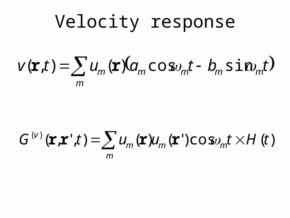
Velocity response

m

mmmmm tbtautv sincos)(),( rr

)(cos)'()(),',()( tHtuutGm

mmmv rrrr

Uncorrelated excitation

m

mmmmm tbtautv sincos)(),( rr

0

2

2

mn

nmmn

nmmn

ba

Fbb

Faa

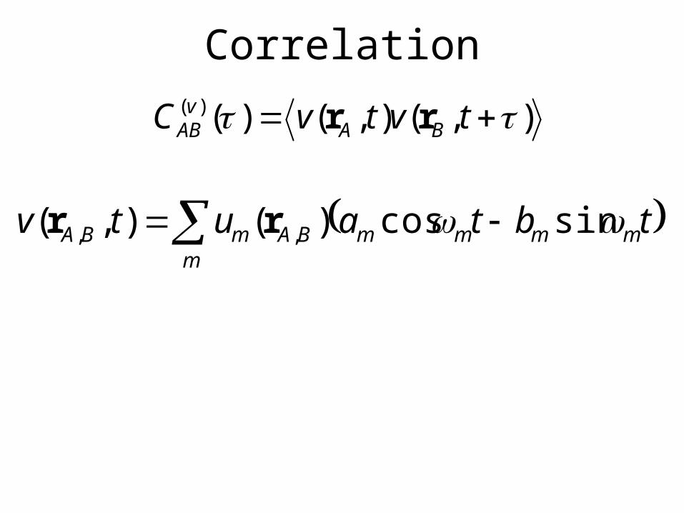
Correlation

),(),()()( tvtvC BAvAB rr

m

mmmmBAmBA tbtautv sincos)(),( ,, rr

Correlation as sum over modes

ttbb

ttab

ttba

ttaa

uuC

mnmn

mnmn

mnmn

mnmn

mnBmAn

vAB

sinsin

cossin

sincos

coscos

)()()(,

)( rr

For uncorrelated modes

ttbb

ttab

ttba

ttaa

uuC

mnmn

mnmn

mnmn

mnmn

mnBmAn

vAB

sinsin

cossin

sincos

coscos

)()()(,

)( rr

nmF 2

For uncorrelated modes

ttbb

ttab

ttba

ttaa

uuC

mnmn

mnmn

mnmn

mnmn

mnBmAn

vAB

sinsin

cossin

sincos

coscos

)()()(,

)( rr

nmF 2

mcos

Correlation

m

mBmAmvAB uuFC cos)()()( 2)( rr

Green’s function

)(cos)()(),,()( HuuGm

mBmAmBAv rrrr

Correlation

m

mBmAmvAB uuFC cos)()()( 2)( rr

Green’s function

)(cos)()(),,()( HuuGm

mBmAmBAv rrrr

0 ),,()( )(2)( BAvv

AB GFC rr

Correlation

m

mBmAmvAB uuFC cos)()()( 2)( rr

Green’s function

)(cos)()(),,()( HuuGm

mBmAmBAv rrrr

0 ),,()( )(2)( BAvv

AB GFC rr

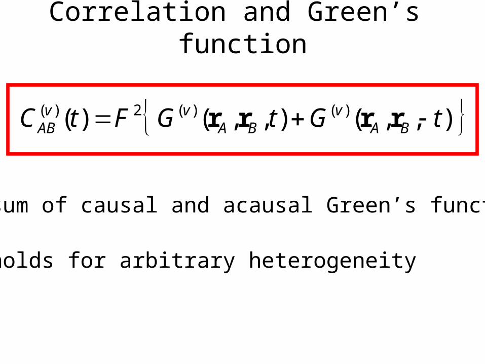
Correlation and Green’s function

),,(),,()( )()(2)( tGtGFtC BAv

BAvv

AB rrrr

- sum of causal and acausal Green’s function

- holds for arbitrary heterogeneity

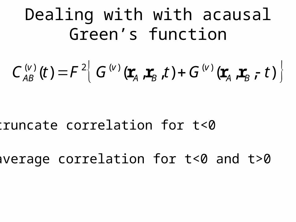
Dealing with with acausal Green’s function

),,(),,()( )()(2)( tGtGFtC BAv

BAvv

AB rrrr

- truncate correlation for t<0

- average correlation for t<0 and t>0

Displacement instead of velocity

2

)(2)(

dt

CdC

dispABv

AB

t

tGtG BA

disp

BAv

),,(

),,()(

)( rrrr

),,(),,()( )()(2)(

tGtGFtdt

dCBA

dispBA

dispdispAB rrrr

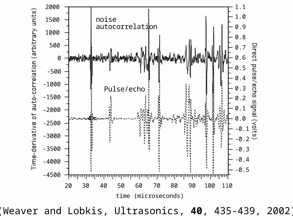
Conclusion: time derivative may appear

(Weaver and Lobkis, Ultrasonics, 40, 435-439, 2002)

20 30 40 50 60 70 80 90 100 110

-4500

-4000

-3500

-3000

-2500

-2000

-1500

-1000

-500

0

500

1000

1500

2000

-0.5

-0.4

-0.3

-0.2

-0.1

0.0

0.1

0.2

0.3

0.4

0.5

0.6

0.7

0.8

0.9

1.0

1.1

time (microseconds)

Pulse/echo

noiseautocorrelation

(Weaver and Lobkis, Ultrasonics, 40, 435-439, 2002)

Representation theorem

Acoustic waves

qpi v

0 vip

Green’s function:

02

21rr

G

cG

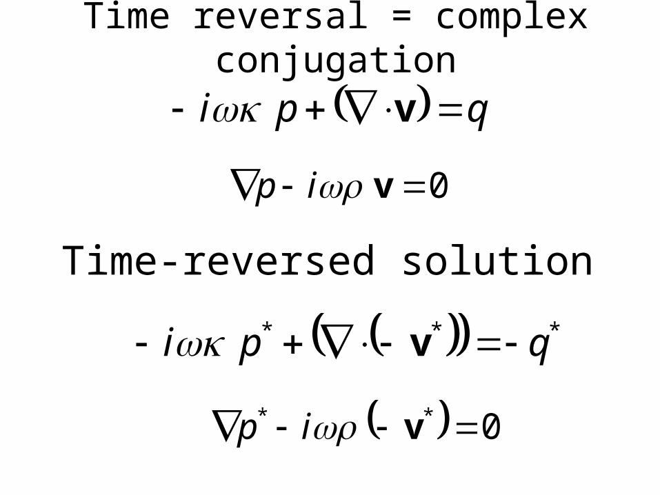
Time reversal = complex conjugation

qpi v

0 vip

*** qpi v

0** vip

Time-reversed solution

Time-reversal

When is a solution.

then is a solution as well

N.B. this does not hold in the presence of attenuation

qp ,, v

*** ,, qp v

Representation theorem

dSppdVpqqp BABABABA nvv ˆ *** ,, AAAAAA qqpp vvreplace:

dSppdVpqqp BABABABA nvv ˆ****

Left hand side

),()()()(

),()()()(

BBBB

AAAA

Gpq

Gpq

rrrrrr

rrrrrr

),(),(

),(),(

*

***

BABA

BAABBABA

rrGrrG

rrGrrGdVpqqp

reciprocity

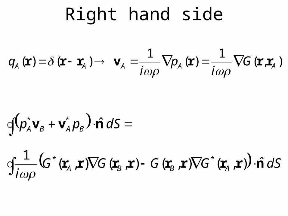
Right hand side

),(1

)(1

)()( AAAAA Gi

pi

q rrrvrrr

dSGGGGi

dSpp

ABBA

BABA

nrrrrrrrr

nvv

ˆ),(),(),(),(1

ˆ

**

**

For spherical surface far away

rrrrr ˆ),(),( BB Gc

iG

dSGGc

dSpp BABABA ),(),(1

2ˆ *** rrrrnvv

Radiation condition:

Virtual-sources

dSGGc

GG BABABA ),(),(1

2),(),( ** rrrrrrrr

Ar

Br

r

(Wapenaar, Fokkema, and Snieder, JASA, 118, 2783-2786 2005heuristic derivation: Derode et al., JASA, 113, 2973-2976, 2003)

Computing synthetic seismograms

(Van Manen et al., Phys. Rev. Lett., 94, 164301,2005)

Field example of virtual sources

(Bakulin and Calvert, SEG expanded abstracts, 2477-2480, 2004)

reservoir

complicated overburden

Peace River 4D VSP

1 0.500.5

1x

10.5

00.51y

1 0.50

0.5

1

z

1 0.500.5

1x

10.5

00.51y

Component used,along-the-well (450)

Image from virtual sources

topbottom

Virtual source Surface

Virtual-sources

dSGGc

GG BABABA ),(),(1

2),(),( ** rrrrrrrr

Ar

Br

r

(Wapenaar, Fokkema, and Snieder, JASA, 118, 2783-2786 2005heuristic derivation: Derode et al., JASA, 113, 2973-2976, 2003)

Excitation by uncorrelated sources on surface

)'(),'(),()()(** rrrrrr FNNc

Uncorrelated sources can be:

- sequential shots

- uncorrelated noise

Response to uncorrelated noise

)()(1

')'()',()(),(1

')',()'(),(1

),(),(1

*2

***2

*

*

BA

BA

BA

BA

ppF

dSNGdSNGF

dSdSGGc

dSGGc

rr

rrrrrr

rrrrrr

rrrr

Green’s function from uncorrelated sources

)()(2

),(),( *2

*BABABA pp

FGG rrrrrr

Ar

Br

r

(For elastic waves: Wapenaar, Phys. Rev. Lett, 93, 254301, 2004)

Raindrop model

Sources can be:

- real sources

- secondary sources (scatterers)

Response to random sources

SS

SS ctStp rr

rrr

/),(

Response to random sources

SBASBA

SSBA ctStp rr

rrr

,

,, /),(

Ar Br

Sr

dttptpC B

T

AAB ),(),()(0

rrCorrelation:

Double sum over sources

''',

)(SSSSSS

ABC

diagonal terms cross-terms

Cross-terms

- vanish on average

- in a single realization:

freedomNTf

11

termsdiagonal

termscross

(Snieder, Phys. Rev. E, 69, 046610, 2004)

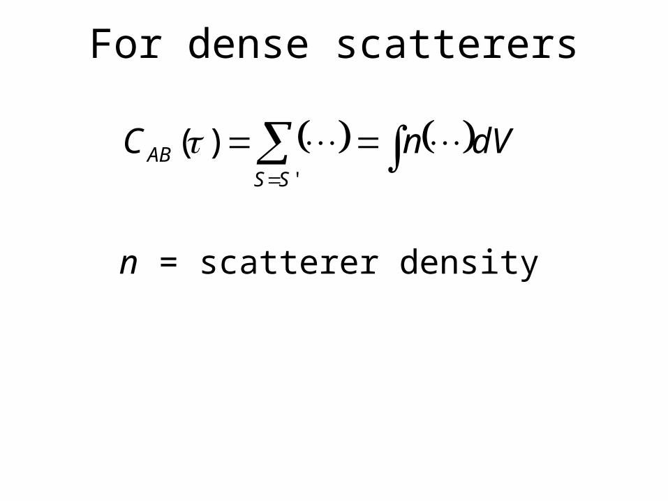
For dense scatterers

dVnCSS

AB '

)(

n = scatterer density

Correlation as volume integral

Ar Br

r

ALBL

dV

LL

LLikSnC

BA

BAAB

exp)()(2

Stationary phase contribution

0zyx

y

z

R

Stationary phase regions

“anti-Fresnel zones”

Stationary phase integration

R

ikRe

R

ikRe

i

cSnCAB

44

)()(

2

)()()(

)( *

2

RGRGi

cSnCAB

(Snieder, Phys. Rev. E, 69, 046610, 2004,for reflected waves see:

Snieder, Wapenaar, and Larner, Geophysics, in press, 2005)

Yet another type of illumination

(Weaver and Lobkis, JASA, 116, 2731-2734)

Four types of averaging

Ultrasound experiment

source

receivers

54 mm

135 mm

(Malcolm et al., Phys. Rev. E, 70, 015601, 2004)

Surface waves

(Campillo and Paul, Science, 299, 547-549, 2003)

correlation Green’s tensor

Z/Z

Z/R

Z/T

correlation Green’s tensor

Z/Z

Z/T

R/ZR/RR/T

T/ZT/R

T/T

Z/R

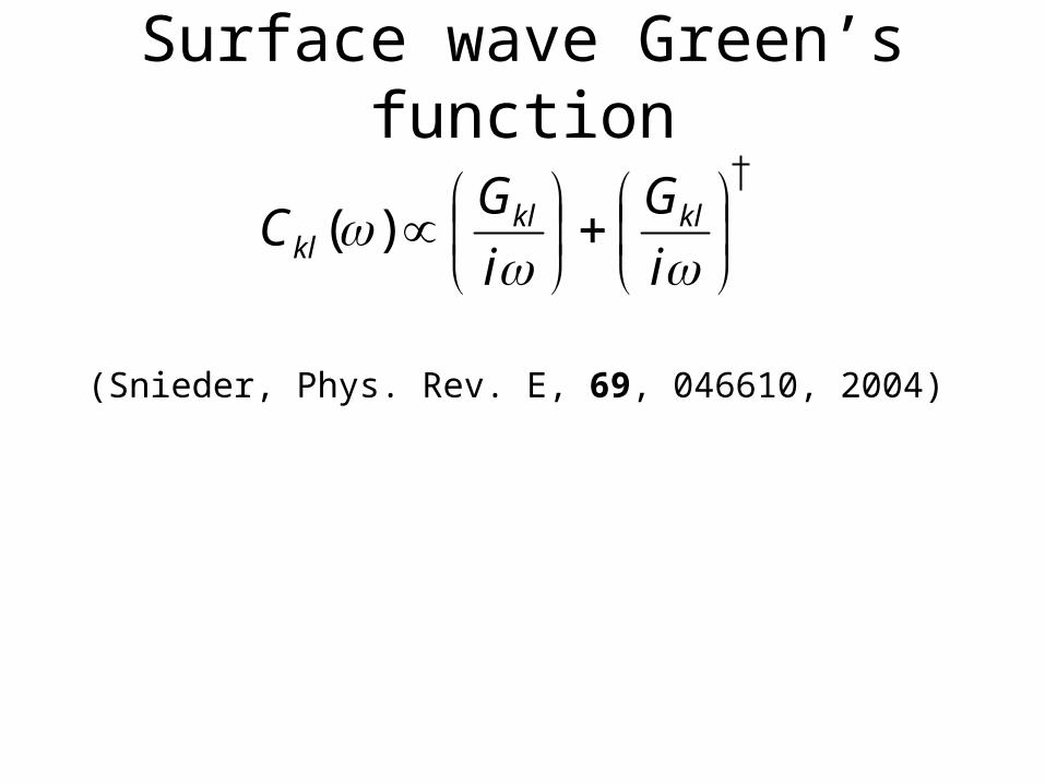
Surface wave Green’s function

i

G

i

GC klklkl )(

(Snieder, Phys. Rev. E, 69, 046610, 2004)

Surface wavedispersionfrom noise

(Shapiro and Campillo,Geophys. Res. Lett.,

31, L07614, 2004)

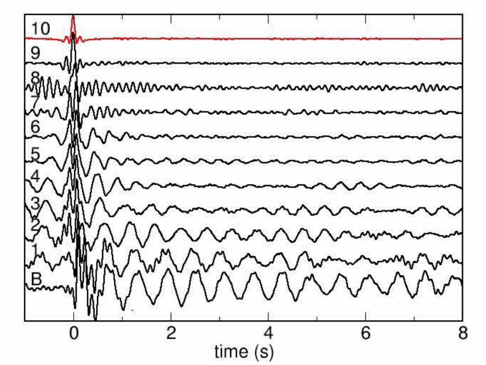
Seismic interferometry in Millikan Library

Deconvolution with top floor

Deconvolution with bottom floor

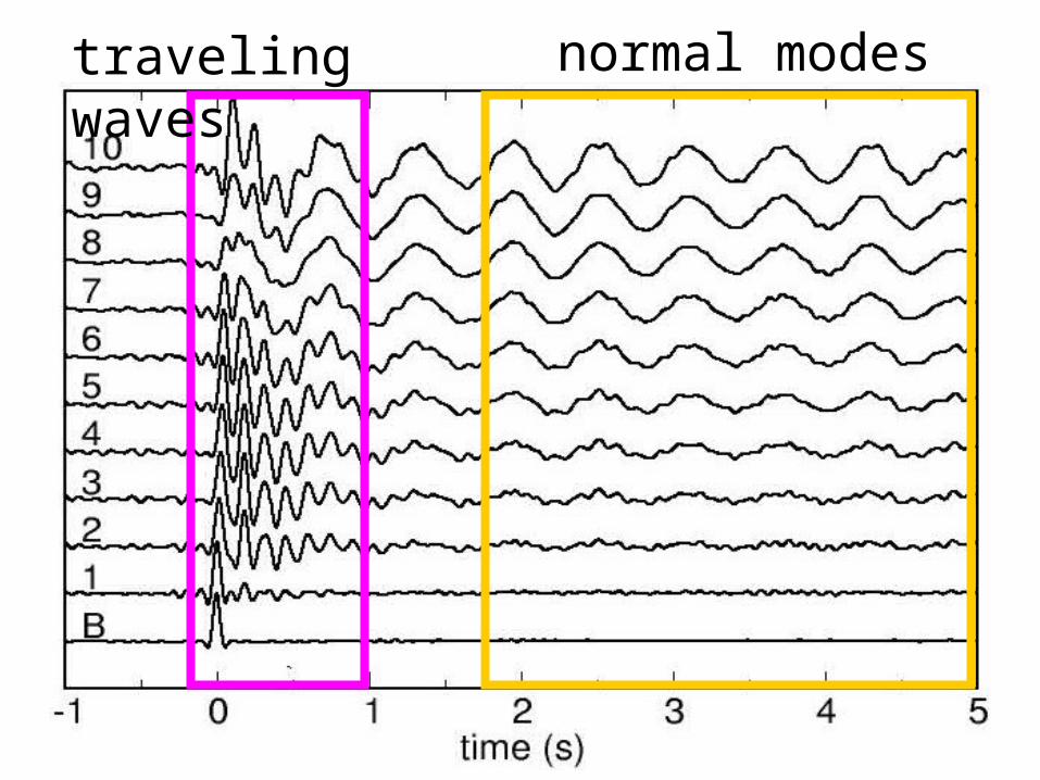
traveling waves normal modes

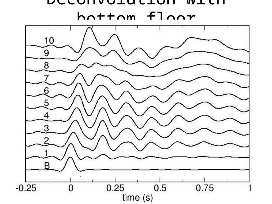
Deconvolution with bottom floor

+ +

Sheiman-interpretation

+ -+ -

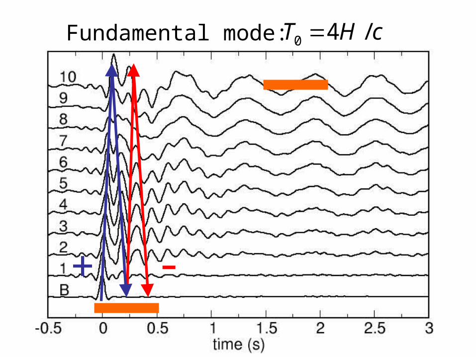
cHT /40 Fundamental mode:

-+

Borehole data from Treasure Island

T – Deconvolved (4.5 to 15 sec)

time (sec)

dep

th (

m)

T – Deconvolved (4.5 to 15 sec)

time (sec)

dep

th (

m)

β

β

β

β

β

=100 m/s=150 m/s

=200 m/s

=250 m/s

=550 m/s

Z – Deconvolved (1 to 15 sec)

time (sec)

dep

th (

m)

Z – Deconvolved (1 to 15 sec)

time (sec)

dep

th (

m)

ααα

α

α

=1500 m/s=1250 m/s

=1600 m/s

=1350 m/s

=2200 m/s

R – Deconvolved (4.5 to 15 sec)

time (sec)

dep

th (

m)

time (sec)

dep

th (

m)

β

β

β

β

β

=100 m/s=150 m/s

=200 m/s

=250 m/s

=550 m/s

R – Deconvolved (4.5 to 15 sec)

Borehole data from Treasure Island

R – Deconvolved (1 to 4.5 sec)

time (sec)

dep

th (

m)

R – Deconvolved (1 to 4.5 sec)

time (sec)

dep

th (

m)

β

β

β

β

β

=100 m/s=150 m/s

=200 m/s

=250 m/s

=550 m/s

Receiver Function

time (sec)

dep

th (

m)

Receiver Function

time (sec)

dep

th (

m)

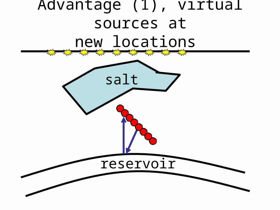
Advantage (1), virtual sources atnew locations

reservoir

salt

Advantage (1), virtual sources atnew locations

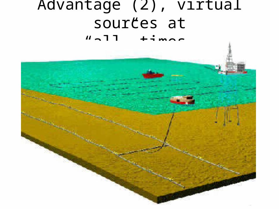
Advantage (2), virtual sources at“all” times

Seismic interferometry in Millikan Library

(Snieder and Safak, Bull. Seismol. Soc. Am., in press, 2005)

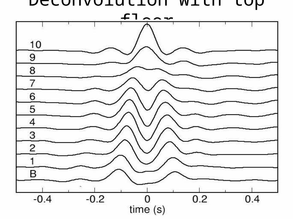
Deconvolution with top floor

Advantage (3), get better illumination

Use surface bounce

Use surface bounce

“Schuster trick”

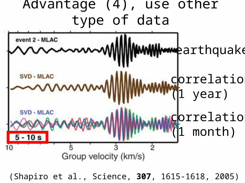
Advantage (4), use other type of data

(Shapiro et al., Science, 307, 1615-1618, 2005)

earthquake

correlation(1 year)

correlation(1 month)

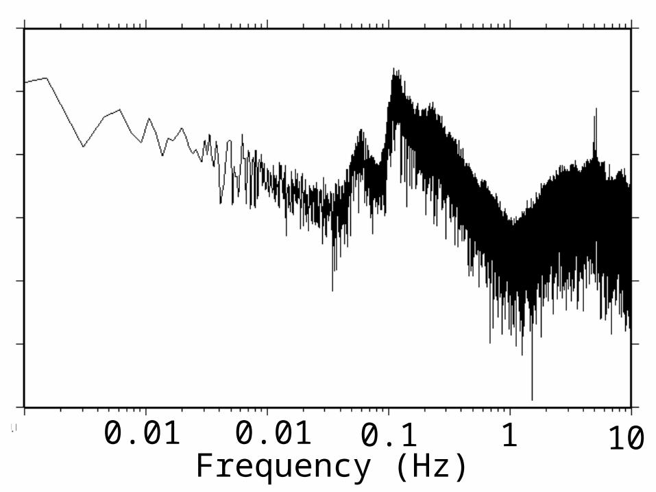
1010.10.010.01

Frequency (Hz)

5-10sec.

1010.10.010.01Frequency (Hz)