seismic interpretation of...
TRANSCRIPT

SEISMIC INTERPRETATION OF PENNSLYVANIAN
ATOKAN STRATA USING 3D SEISMIC INVERSION
DATA, WILBURTON GAS FIELD, ARKOMA BASIN,
SOUTHEASTERN OKLAHOMA
By
CHRISTINE ROBIN HAGER
Bachelor of Science in Geology
Oklahoma State University
Stillwater, Oklahoma
2007
Submitted to the Faculty of the Graduate College of the
Oklahoma State University in partial fulfillment of
the requirements for the Degree of
MASTER OF SCIENCE May, 2009
i
SEISMIC INTERPRETATION OF PENNSLYVANIAN
ATOKAN STRATA USING 3D SEISMIC INVERSION
DATA, WILBURTON GAS FIELD, ARKOMA BASIN,
SOUTHEASTERN OKLAHOMA
Thesis Approved:
Dr. Ibrahim Cemen
Thesis Adviser
Dr. James Puckette
Dr. William Coffey
Dr. A. Gordon Emslie
Dean of the Graduate College

ii
ACKNOWLEDGMENTS
The completion of this thesis was not possible without the help of many people
and organizations.
First, I would like to thank Devon Energy Corporation for all they do for the
Boone Pickens School of Geology at Oklahoma State University. Devon Energy donated
the data that was used for this thesis and provided me with a learning experience that will
be very applicable to industry. Rod Gertson has been a great resource with his
geophysical expertise. I would like to thank him for sacrificing his own time to answer
questions and aid in the completion of this thesis. Dr. Bill Coffey was an invaluable
resource with all of his experience working the Arkoma Basin. Laura Dewett was a great
help with data loading and providing me with well data and technical support for this
project.
Seismic Micro Technology (SMT) has generously given the OSU Boone Pickens
School of Geology a license to run their software KINGDOM Suite. This program was
the main software used for the completion of this project and without this grant this thesis
would not have been possible. Their technical support was very helpful and played an
essential role in completing this M.S. thesis.
I would also like to thank Gorka Garcia of Odegaard America Inc. who was very
helpful in answering questions about this inversion and the process of inversion.

iii
I would like to thank my advisor, Dr. Ibrahim Cemen. His insight about the study
area was very helpful through the entire process. His understanding of structural geology
has provided me with knowledge that is invaluable. I would also like to thank Dr. Jim
Puckette for his help with this project. His well log expertise has provided me with
knowledge that will set me ahead in the working world. I would also like to thank
ExxonMobil for offering me an internship. This internship provided me with an
invaluable learning experience from which I was able to use some of the learned concepts
and apply them in my own thesis. Finally, I would like to thank my friends and family.
Their support helped keep me motivated through this process and made it much more
pleasant.
Again I would like to thank everyone who helped make this thesis possible. I
would never have finished without your help and support. Thank you.

iv
TABLE OF CONTENTS
Chapter Page I. INTRODUCTION ......................................................................................................1
Study Area ...............................................................................................................4 Purpose of Study ......................................................................................................4 Methodology ............................................................................................................6 II. GEOLOGIC OVERVIEW OF THE ARKOMA BASIN TECTONICS AND STRUCTURAL GEOLOGY………………………………………………….…8 III. STRATIGRAPHY OF THE ARKOMA BASIN ..................................................14 Pre-Pennsylvanian Rock Units ..............................................................................14 Pennsylvanian Rock Units .....................................................................................18 IV. SEDIMENTOLOGY OF THE WAPANUCKA LIMESTONE AND SPIRO
SANDSTONE ........................................................................................................22 Diagenetic History .................................................................................................26 V. REFLECTION SEISMOLOGY .............................................................................31
Theory…………………………………………………………………………….32 Acquisition .............................................................................................................34 Processing ..............................................................................................................38 Interpretation. .........................................................................................................41 VI. SEISMIC INVERSION .........................................................................................47
Theory ....................................................................................................................48 Process of Inversion ...............................................................................................51 Seismic Acoustic Impedance versus Well Log Acoustic Impedance…………….52

v
Chapter Page
VII. INTERPRETATION OF THE SEISMIC INVERSION DATA ..........................61 Structure .................................................................................................................64 Porosity ..................................................................................................................74 Thickness ...............................................................................................................78 VIII.CONCLUSION ....................................................................................................87 REFERENCES ............................................................................................................92

vi
LIST OF FIGURES
Figure Page
1. Location of the study area along the Ouachita Thrust Belt………………………..2
2. Location of the study area on the edge of the Frontal Ouachitas ……………..…..5
3. Paleogeographic maps and cross-sections depicting the evolution of the Arkoma Basin…………………………………………………………………..….9
4. Cross-section of Wilburton Gas Field illustrating the Triangle Zone……………11
5. Stratigraphic nomenclature of the Arkoma Basin……………………………....15
6. Stratigraphic chart illustrating amounts of deposition during different time
frames…………………………………………………………………………….16
7. Detailed stratigraphic nomenclature lower Pennsylvanian Subsytem…………....19
8. Isopach map showing Foster Channel complex……………………………….....25
9. Paleogeographic map showing deposition of Wapanucka Limestone and Spiro Sandstone………………………………………………………………………....27
10. Porosity versus chamosite crossplot……………………………………………...29
11. Common Midpoint field Procedure……………………………………………....36
12. Attenuation losses of the seismic signal………………………………………….37
13. Normal Moveout correction (NMO)……………………………….………….....39
14. Semblance Plot Example for picking velocities………………………………….40
15. Example of Kirchoff migration………………………………………………......42
16. Zero phase wavelet versus mixed phase wavelet………………………………...44
17. Phase reversal using AVO analysis………...……………………….………...….46

vii
Figure Page
18. Schematic example of inversion…..………………………………………….…..50
19. Basic workflow of seismic inversion…………………………....………………..53
20. Wavelet extraction at well 1 ……………………………….……………….…....54
21. Crossplot of acoustic impedance derived from seismic vs. calculated acoustic impedance derived from well logs………………………………….…...57
22. Discrepant low frequency model tie at well 4………………………………...….58
23. Bad calculated impedance ties to seismic…………………………………....…...60
24. Synthetic tie at well 1 on convention 3D data……………………………..……..62
25. Acoustic impedance curve tie on inversion 3D data………………………….….63
26. Location of four different thrust sheets analyzed in the study area……………....65
27. Two thrusts of Spiro Sandstone penetrated in well 3 illustrating synclinal
and anticlinal folding…………………………………………………………..…67
28. Crossplot of velocity versus porosity for two thrusts of Spiro Sandstone in well 3…………………………………….………………………................….68
29. Horizon contour map of the Spiro Sandstone thrust sheet 2……………….…….69
30. Arbitrary lines drawn to illustrate areas of tighter folds shown on Figure 29…....70
31. Average velocity for Spiro Sandstone for all wells with sonic curves…………...71
32. Crossplot of acoustic impedance vs. velocity in the Spiro Sandstone.…………...72
33. Cross-section of conventional seismic showing faulting in well 2……………….74
34. Crossplot of acoustic impedance versus density porosity for well 2 and
Well 1 …………....…………………………………………………………….....75
35. Porosity versus Impedance crossplot example used in industry Columbia………………………………………………………………………….76
36. Crossplot of acoustic impedance and porosity comparing well 1 and
Well 2 ……….………………………………………………………………........77

viii
Figure Page
37. Well 5 sonic curve over Spiro Sandstone showing facies change………………..79
38. Map of acoustic impedance of Spiro Sandstone thrust sheet 2……………….….80
39. Location of arbitrary line on base map illustrating changes in acoustic impedance over the survey…………………………………………...81
40. Location of arbitrary line number two on base map illustrating changes in
acoustic impedance over the survey……………………………………………...82
41. Isochron map of Spiro Sandstone thrust sheet 2………………………………….84
42. Crossplot of seismic thickness versus well thickness in Spiro Sandstone………..85
43. Area of interest located on amplitude map……………………………………….90
44. Areas of interest located on isochron map………………………………………..91

1
CHAPTER I
INTRODUCTION
The Arkoma Basin is a foreland basin formed during the Pennsylvanian Ouachita
Orogeny. It is located in southeastern Oklahoma and extends east into the western part of
Arkansas. The Arkoma Basin is approximately 250 miles long and about 50 miles wide.
During the Ouachita Orogeny, collision of the North American Plate and a southern
landmass known as Llanoria formed the Arkoma Basin and Ouachita mountains
(Houseknecht and Kacena, 1983). The Pennsylvanian Ouachita Orogeny is also
responsible for the generation of other foreland basins such as the Black Warrior and Fort
Worth, which all lie landward along the Ouachita fold thrust belt (Figure 1). These basins
are related both stratigraphically and tectonically (Branan, 1968).
Foreland basins are extensively researched across the world because of their
reservoir potential. The Arkoma Basin is one of many prolific foreland basins in North
America. The first discovery of natural gas in the Arkoma Basin was in 1902, but
extensive drilling did not begin until deeper Atokan sandstones were reached (Branan,
1968). The Spiro Sandstone is one of the lower Atokan deeper sandstones that is an
exceptional reservoir in the basin and is distributed over a large area (Branan, 1968, and
Cemen et al., 2001).

2
Figure 1. Yellow circle indicating the approximate location of thesis study area within the Arkoma Basin along the Ouachita thrust belt (after Branan, 1968).

3
The Wilburton gas field is one of the many gas fields discovered in the Arkoma
Basin. The field first produced from deeper Atokan reservoir rocks in 1960 with
production in the Spiro Sandstone (Tilford, 1990). The Wilburton gas field is mainly
located in Latimer County, but also extends into the eastern part of Pittsburg County in
Oklahoma. Over 1.3 trillion cubic feet of gas (tcf) has been produced in the Wilburton
gas field and most of it is structurally trapped in the Spiro Sandstone. Over 733 billion
cubic feet of gas (bcf) has been produced in the 3D survey study area. These values are
current as of February 2008 (IHS, 2008).
Many M.S. theses have been completed covering the geology of the Arkoma
Basin over the years at the Oklahoma State University Boone Pickens School of Geology.
Most focused on the stratigraphy and structural features of the basin. Recently a M.S.
thesis was completed by William Parker (2007) in which a 3D conventional seismic data
set was interpreted. This thesis provided a better understanding of the some of the
structural relationships present in the Arkoma Basin. Additionally, seven cross sections
were constructed and balanced to determine the amount of shortening in the Spiro
Sandstone by Wahab Sadeqi (2007) for a M.S. thesis project completed in Spring 2007.
The 3D conventional data set used by William Parker has since been inverted to acoustic
impedance, and is now being used for this research to interpret stratigraphic relationships.
This thesis will study the rock properties of the Spiro Sandstone by establishing
relationships between acoustic impedance and porosity.

4
STUDY AREA
The Ouachita Mountains are commonly subdivided into three sections: from north
to south they are the Frontal Belt, Central Belt, and Broken Bow Uplift (Figure 2). These
subdivisions are made based on their location from the continent interior. The Frontal
Belt is the closest to the continental interior and is dominated by imbricate reverse faults.
The Central Belt contains large synclines and fewer reverse faults. The Broken Bow
Uplift, most southern section and farthest from the continent interior, contains tight
overturned folds (Feenstra and Wickham, 1975). The frontal Ouachitas are highly
deformed and are separated from the mildly deformed foreland Arkoma Basin by the
Choctaw Fault. The Wilburton triangle zone partitions the mildly deformed strata from
the highly deformed strata. The study area is marked in Figure 2 and is located in the
Wilburton gas field, which is located in the transition zone between the mildly deformed
strata of the Arkoma Basin and the tightly deformed strata of the Frontal Belt (Cemen et
al., 2002).
PURPOSE OF STUDY
The main purpose of this study is to use proprietary 3D seismic that has been
calibrated to well control to tie acoustic impedance changes to porosity changes in the
Spiro Sandstone. This 3D seismic data set has been inverted to acoustic impedance; the

5
Figure 2. Study area location in the Arkoma Basin on the edge of the Frontal Ouachitas (after Cemen et al., 2001). Box 1: Middle Paleozoic (Cambrian through Early Mississippian). Box 2: Middle to late Mississippian (Stanley Group of Ouachitas) Box 3: Morrowan (Jackfork Group and Stanley Formation of Ouachitas) Box 4: Atokan (Spiro/Wapanucka and Atoka Formations of the Ouachitas and Arkoma Basin) Box 5: Desmoinesian (Hartshorne, McAlester, Savana, and Boggy Formations of the Arkoma). H=town of Hartshorne, W=town of Wilburton, WL=Wister Lake
STUDY AREA

6
product of multiplying density by velocity, which can be used to map property changes in
the rocks. A few rock properties that can affect acoustic impedance are porosity, fluid
content, clay content and cementation. For example, a porous rock will be less dense and
have a slower velocity, giving lower acoustic impedance compared to a rock that is
tightly cemented, which will be faster and have a higher density. In areas where well
control is
lacking, this relationship between acoustic impedance and porosity may help identify
more productive areas. Seismic acoustic impedance can also be used to map thickness
changes and help identify thin beds not resolved with conventional seismic data. In
earlier work at OSU (Parker, 2007 and Sadeqi, 2007), the Spiro Sandstone and the
Wapanucka Limestone, which underlies the Spiro Sandstone, were analyzed as a
package. The inversion data shows a large acoustic impedance contrast between the Spiro
Sandstone and Wapanucka Limestone, allowing the two units to be analyzed
independently. Formation tops were also picked more accurately with the inverted
seismic data. This acoustic impedance data set was used to map thickness changes in the
Spiro Sandstone and map areas of higher porosity in the survey area.
METHODOLOGY
In 2000, a 3D seismic data set was acquired in Pittsburg and Latimer counties
within the Wilburton gas field. This 3D data set was donated by Devon Energy
Corporation to the OSU Boone Pickens School of Geology to be used for M.S. thesis

7
projects. This data set was then inverted to acoustic impedance by Odegaard America
Inc. in 2005. Interpretation of this data is being done in KINGDOM Suite version 8.1,
a software package from Seismic Micro-Technology (SMT). Picked horizons and major
faults were interpreted by Parker (2007) on a conventional reflection seismic data set
calibrated to well control. Since then, using the acoustic impedance data set, two
additional horizons were picked. Well logs and acoustic impedance values taken from the
seismic data were crossplotted to derive relationships between porosity and acoustic
impedance. The following steps were used to carry out interpretations on the data:
1) 3D seismic inversion data was imported into KINGDOM Suite version 8.1.
2) Log Ascii Standard (LAS) files with logs and formation tops were imported bringing
the total wells in the project to 64.
3) Time-Depth charts were created using sonic logs to change depth values into time
values so that calculated acoustic impedance curves in depth can be tied to the seismic.
4) Calculated acoustic impedance curves were tied to the impedance data to calibrate well
data to seismic data.
5) The base of the Spiro/ top of the Wapanucka and base of the Wapanucka were picked
over the survey by hand using the picking tool in KINGDOM Suite v. 8.1
6) Wells with sonic logs were identified and velocities were compared over the survey
area.
7) Relationships were established between porosity and acoustic impedance. Areas of
higher porosity in the Spiro Sandstone correlated to lower acoustic impedance values.
8) Seismic thickness and amplitude maps for the Spiro Sandstone were created to
compare impedance changes over the area.

8
CHAPTER II
GEOLOGIC OVERVIEW OF THE ARKOMA BASIN TECTONICS AND
STRUCTURAL GEOLOGY
The Arkoma Basin is a foreland basin bounded to the south by the Ouachita
Mountains, to the north by the Ozark Uplift, to the northwest by the Oklahoma/Cherokee
Platform, to the west by the Hunton Arch, to the southwest by the Arbuckle Mountains,
and to the east by the Reelfoot Rift/Mississippian Embayment. The sedimentary rock
thickness ranges from 3,000 feet on the northern shelf of the basin to 30,000 feet along
the frontal Ouachita Mountains to the south (Branan, 1968 and Johnson, 1988).
The Arkoma Basin began forming as a result of the opening and closing of an
early Paleozoic ocean in the Mid-Cambrian (Houseknecht and Kacena, 1983) (Figure 3).
Rifting began during the early Paleozoic, which resulted in the failed rift arms creating
the Southern Oklahoma Aulacogen and Reelfoot Rift. The Paleozoic ocean started to
close during the Late Devonian to Early Mississippian when Llanoria began encroaching
on the southern margin of North America. A subduction zone was created during the
Devonian, which is supported by the presence of arc-related volcanic debris in the
Mississippian aged Stanley Shale. During this time a basin formed and accumulated
sediment derived from the Central Appalachians to the north and northeast. During the
Devonian to Mississippian an accretionary prism developed. This prism abducted onto
the continental margin of North America during the Atokan, which later
9
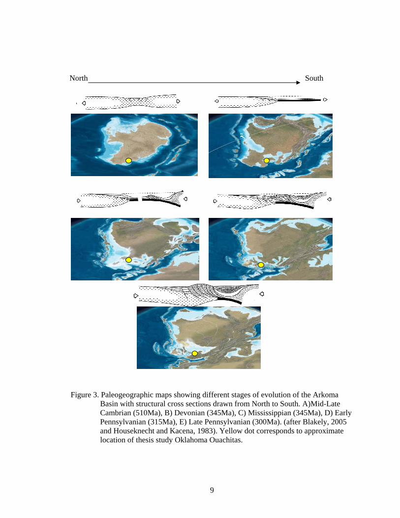
Figure 3. Paleogeographic maps showing different stages of evolution of the Arkoma Basin with structural cross sections drawn from North to South. A)Mid-Late Cambrian (510Ma), B) Devonian (345Ma), C) Mississippian (345Ma), D) Early Pennsylvanian (315Ma), E) Late Pennsylvanian (300Ma). (after Blakely, 2005 and Houseknecht and Kacena, 1983). Yellow dot corresponds to approximate location of thesis study Oklahoma Ouachitas.
North South

10
became the Ouachita Mountains. During this time, flexural bending of the overriding
plate caused normal faults, originally formed in the Cambrian to Devonian, to be
reactivated, deepening the basin and causing an abrupt increase in the thickness of
sediments (Branan, 1968, Houseknecht and Kacena, 1983, and Johnson, 1988).
As discussed previously the Ouachita Mountains can be separated into three belts;
Frontal Belt, Central Belt, and the Broken Bow uplift; based on both stratigraphy and
structural style. The Frontal Belt lies between the Choctaw and Winding Stairs fault and
consists of steeply tilted, imbricately thrusted and tightly folded strata, shallow water
Morrowan basinal strata. The Central Belt has broad open synclines, separated by tight,
typically thrust-cored anticlines. The Broken Bow Uplift consists of isoclinally folded
and thrusted Early Ordovician to Early Mississippian deep-water strata (Suneson and
Hemish, 1994).
The Wilburton gas field and surrounding areas contain down-to-the-south normal
faults that are evident on the northern part of the cross-section (Figure 4) which was
constructed by Cemen (2001). These faults formed in the north end of the leading
imbricate thrust of the duplex structure (Figure 4). Normal faults show a maximum 2,000
feet dip separation. These normal faults are assumed to be formed as growth faults based
on two lines of evidence (1) the abrupt increase in thickness of the middle and lower
Atoka; and (2) presence of turbidite-facies present in the lower and middle Atoka.
Normal faults in Pre-Pennsylvanian rocks may have acted as barriers that forced the
thrusts to ramp over basement rocks (Houseknecht and Kacena, 1983).

11
Figure 4. Wilburton gas field triangle zone interpretation (after Cemen et al., 2001). CF=Carbon Fault, CHF=Choctaw Fault, PMF= Pine Mountain Fault, TVF= Ti Valley Fault and LAD=Lower Atokan Detachment.

12
In the early 1990’s funding became available to fund research on the subsurface
structural styles of the Arkoma Basin. Cemen et al. (2001) proposed a well developed
triangle zone in the Wilburton gas field area. Two major faults and one detachment
surface comprise the triangle zone located in Wilburton gas field. The triangle zone
(Figure 4) is formed by the southerly dipping Choctaw fault, forming one side of the
triangle, and the northerly dipping Carbon fault, forming the other side of the triangle.
The triangle is floored by the Lower Atokan Detachment Surface (LAD) (Cemen et al.,
2001).
The Choctaw fault is a west-southwest to east-northeast striking and southerly
dipping thrust fault that extends more than 120 miles in Oklahoma. The hanging wall of
the Choctaw fault contains many asymmetrical or overturned folds that are also found in
the hanging walls of other thrust faults including the Ti Valley and Pine Mountain faults
(Cemen et al., 2001).
The Ti Valley Fault is a major thrust fault extending 240 miles from near Atoka,
Oklahoma to Jacksonville, Arkansas. The Ti Valley trends west-southwest to east-
northeast with a southeasterly dip of 70-80º. The Pine Mountain fault strikes west-
southwest to east-northeast and is subparallel to the Ti Valley fault. The Pine Mountain
fault dips 70-80º to the south, loses dip with depth and is a splay from the Woodford
detachment or the Choctaw fault. This interpretation was determined by seismic profiles
and wire-line log data (Cemen et al., 2001).
The Carbon fault is an east-west striking fault. It dips to the north approximately
30-40º. The Carbon fault has been interpreted as formed by the continued upward and
northward propagation of the roof thrust, or Lower Atokan Detachment (LAD), within

13
the shales of the Atoka. The incompetent shale units cause the LAD to propagate with a
low angle and form a gentle ramp. When the detachment reached a zero-displacement
point it encounters a hindrance to its forward (northward) movement and begins to form a
backthrust. The Carbon fault formed in this way to accommodate back thrust movement
in the area (Cemen et al., 2001).
Shortening calculations were applied to the Spiro Sandstone/Wapanucka
Limestone in the Wilburton triangle zone (Cemen et al., 2002). The Spiro Sandstone/
Wapanucka Limestone was used as the key bed for restoration because a) it has a very
recognizable well-log signature and b) it is the only competent rock unit found in both the
footwall and hanging wall of the Choctaw fault zone. The amount of shortening in the
Wilburton triangle zone was calculated to be about 60%. Parker (2007) found shortening
in the Spiro Sandstone in the footwall of the Choctaw fault to be about 22%-29%. These
shortening values were consistent with earlier work by Collins (2006) and Sahai et al.
(2007).

14
CHAPTER III
STRATIGRAPHY OF THE ARKOMA BASIN
The Arkoma Basin contains sedimentary rocks that date from the Cambrian to the
middle Pennsylvanian (Figure 5). Deposition in the Arkoma Basin occurred in three
unique depositional periods dating back to the Cambrian. The earliest depositional period
existed from the Cambrian to Early Atokan and consisted of miogeoclinal deposits,
which contributed 5,000 feet to the total strata (Houseknecht and McGilvery, 1990)
(Figure 6). The Middle-Late Atokan strata were a result of syn-depostitional growth fault
movement accounting for 18,000 feet of strata. The Pennsylvanian Desmoinesian Series
deposition occurred during the late stages of the basin development and accounts for
8,000 feet of strata (Houseknecht and Kacena, 1983).
Pre Pennsylvanian Rock Units
Pre-Pennsylvanian deposition was fairly continuous except for two major
epeirogenic uplifts that occurred during the Early and Late Devonian. Pre-Pennsylvanian
rock units range in thickness from 1,000 feet to about 6,000 feet of sediment at most in
the Arkoma Basin (Johnson, 1988). The Arkoma Basin is floored by a Proterozoic

15
Figure 5. Stratigraphic Nomenclature of the Arkoma Basin (Modified after Johnson, 1988).
Granite and rhyolite
Baylock Sandstone
Proterozo ic
Upper
Lower
Middle
Upper
Cambrian
Ordovician
Silurian Devonian
Mississippian
Pennsylvanian
Series Arkoma Basin Ouachita Mountains
Desmoinesian
Atokan
Morrowan
Chestarian
Meramecian
Osagean
Kinderhookian
Upper
Lower
Upper
Lower
Krebs Group Boggy Fm.
Savanna Fm.McAlester Fm.
Hartshorne Fm. Upper
LowerAtoka Fm.
“Caney” Sh.
Woodford Sh.
Hunton Gp.
Frisco Ls. Bois d’Arc Ls.Haragan Ls.Henryhouse Fm.
Chimneyhi llSubgroup
Sylvan Sh.
Viola
Gp.
Simpson
Gp.
Arbuckle
Gp.
Timbered
Hills Gp.
Welli ng Fm.Vi ola Spri ngs Fm.Bromi de Fm.Tulip Creek Fm.McLish Fm.Oil Creek Fm. Joi ns Fm.West Spring Creek Fm.Ki ndblade Fm.Cool Creek Fm.McKenzie Hi ll Fm.Butterly Dol.Si gnal Mountain Ls.Royer Dol.Fort Sill Ls.Honey Creek Ls.
Reagan Ss.
Wapanucka Ls.Union Valley Ls.Cromwell Ss.
Atoka FormationJohns Valley ShaleJackfork Group
Stanley Shale
Arkansas Novaculite
PinetopChert
Missouri Mountain Shale
Polk Creek Sandstone
Bigfork Chert
Womble ShaleBlakely SandstoneMazarn Shale
Crystal Mountain Ss.Collier Shale
? ? ?
Ovs
DSOhs
MD
subsystem
subsystem

16
Figure 6. Stratigraphic chart and time frames illustrating sedimentary rock thickness
during the evolution of the Arkoma Basin (Houseknecht and McGilvery, 1990).

17
crystalline basement. Resting unconformably above the basement rocks is the Reagan
Sandstone which is the widespread basal sedimentary unit in the area. The Lower
Ordovician consists primarily of the Arbuckle Group that represents deposition in a
shallow marine environment as evident by the abundant invertebrate fossils. The Middle
Ordovician is primarily the Simpson Group, which contains shoaling-upwards sequences
(Ham, 1969). The Middle to Late Ordovician contains the Viola Group and consists
mainly of shallow marine carbonates. The Late Ordovician is represented by the Sylvan
Shale, which is thought to represent a shallow marine environment, and the Keel
Formation of Chimneyhill Subgroup of the Hunton Group (Sutherland, 1988).
The Silurian and Lower Devonian are contained within the Hunton Group which
rests unconformably on the Sylvan Shale and is mainly limestone. An epeirogenic uplift
causes a major unconformity separating the Hunton Group from the overlying Woodford
shale (Johnson, 1988). The Late Devonian/Early Mississippian Woodford Shale is a
black, organic rich shale (Ham, 1969). Woodford sediments were deposited in a deep
marine setting (Suneson et al., 2005).
Conditions changed drastically during the Mississippian as thick turbidites were
deposited in the basin (Sutherland, 1988). Mississippian strata include a black, organic-
rich shale known as the Caney Shale. Late Mississippian Springer Shale serves as a major
detachment surface between extensional dominated tectonics and compressional tectonics
of the Pennsylvanian. Other shales comprise the Upper Mississippian Chesterian Series
shale, but they are not well understood (Johnson, 1988). Sediment transport was thought
to come from the southeast during this time (Sutherland, 1988). At the end of the
Mississippian, the sea began to regress because of the broad upwarping of the

18
transcontinental arch, the relative sinking of the Ouachita trough, as well as the
upwarping of the Ozark dome; which all corresponded to the southward tilt of the
Arkoma shelf north of the trough. This was all occurring as the southern landmass known
as Llanoria was encroaching upon the North American plate. Due to the collision, the
Chesterian Series was progressively truncated creating a regional angular unconformity at
the base of the Pennsylvanian (Houseknecht and Kacena, 1983 and Sutherland, 1988).
Pennsylvanian Rock Units
The Pennsylvanian rock units are some of the most noted and studied systems in
the basin because of the highly productive reservoir sands that were deposited during this
time. The series include in order of oldest to youngest; Morrowan Series, Atokan Series,
and Desmoinesian Series (Figure 7) In the beginning of the Morrowan, the sea began to
transgress north onto the Arkoma Shelf across the truncated Chesterian Series surface
(Sutherland, 1988).
Deposition during the Morrowan created large changes in facies and thickness of
sediments. In the eastern part of the basin, the facies consisted of fluvial sandstones and
shales, but moving westward into Oklahoma the facies were mainly mixed shallow-
marine offshore bank facies. In the western part of the basin there is an increase in
limestone and a decrease in sandstone. The Morrowan Series consists of Cromwell
Sandstone and Wapanucka Limestone. The Cromwell Sandstone is considered as the base
of the Morrowan by many workers of subsurface data (Sutherland, 1988). The sandstone

19
Figure 7. Detailed stratigraphic chart of the Pennsylvanian Subsystem showing
informal units within the Arkoma Basin. Spiro Sandstone is boxed in yellow, red arrow indicates detachment surface, and wavy line illustrates unconformity between Morrowan and Atokan (Modified Sutherland, 1988).
Springer Shale
Cromwell Sandstone
Union Valley Limestone
Wapanucka Limestone
Mor
row
an
Penn
sylv
ania
n Su
bsys
tem
Atok
an
Low
er Spiro Sandstone
Foster Sandstone
Ato
ka F
orm
atio
nM
iddl
e
Red Oak SandstonePanola SandstoneDiamond SandstoneBrazil SandstoneCecil SandstoneShay Sandstone
Mis
s.
Che
star
ian
Upp
er Webbers Falls SandstoneGilcrease SandstoneFanshawe Sandstone
Des
moi
nesi
anH
arts
horn
e Fo
rmat
ion
McA
lest
er F
orm
atio
n
Keota SandstoneTamaha Sandstone
Cameron SandstoneBooch Sandstone
Hartshorne Sandstone

20
is fine-medium grained calcareous sandstone overlain by a limestone. The thickness is
more than 35m in the western portion of Oklahoma (Sutherland, 1988). The Union
Valley Limestone is a fossiliferous limestone positioned between the Cromwell
Sandstone and the Wapanucka Limestone.
Deposition between the base of the Atokan Series and the top of the Morrowan
series was interrupted by a drop in sea level that exposed the Morrowan shelf. Foster
channels that were active during the Pennsylvanian incised into the Wapanucka
Limestone, creating an unconformity between the Spiro Sandstone and the Wapanucka
Limestone (Fritz and Hooker, 1994). The Atokan Series consists of the lower, middle and
upper members. The thickness ranges from 305-400m in the northern margin of the
Arkoma Basin in Arkansas to much thicker in the southern margin (Sutherland, 1988).
The lower part of the Atokan Series was deposited in a calm shallow marine setting with
slow sedimentation rates. However, the Middle and Upper Atokan Series sediment were
deposited rapidly in a turbulent marine-nonmarine environment (Houseknecht and
McGilvery, 1990). The Middle Atokan is marked by a drastic increase in thickness due to
syn-depositional growth faults.
The Middle Atokan is characterized by the flexural bending of the southern
margin of the Arkoma shelf. Basin collapse caused flexural bending leading to the
formation or reactivation of previously formed faults that are east-trending syn-
depositional faults. The Middle Atokan rock units thicken on the down-thrown side of
fault blocks due to growth faulting (Sutherland, 1988). This unit consists of mainly shale
and a few sandstones that represent rapid deposition. One of the important sandstone
bodies in this predominately shale rich section is the Red Oak (Houseknecht and

21
McGilvery, 1990). The Red Oak Sandstone is one of the several sandstones that
comprise the Middle Atokan Series. Vedros and Visher (1978) proposed that the Red Oak
Sandstone may be the result of deposition in a submarine-fan environment. However,
Houseknecht and McGilvery (1990) suggests that the sandstone represents deposition in
shallow water because of the continuity of some of the sandstone and the lack of
erosional truncations on up-thrown sides of fault blocks.
Sedimentation rates slowed in the Late Atokan because syn-depositional faults
were no longer active. Deltaic systems that show southward progradation were
transporting sediment from the north and east (Sutherland, 1988).
The Desmoinesian Series is represented by the Krebs Group in the study area,
which is the only rock unit that formed as a result of deposition during major subsidence
and before uplift of the Ouachita fold belt (Houseknecht and McGilvery, 1990). Andrews
and Suneson (1999), proposed that the depositional environments of the Hartshorne
Sandstone, prominent member of the Krebs Group, range from distributary channels,
incised valleys, interdistributary bays, delta margin/ shallow marine, and peat bogs.
The Wapanucka Limestone and the Spiro Formation are the main rock units
studied in this thesis. Seismic acoustic impedance data was used to analyze rock property
changes over the survey area. Therefore, sedimentation and stratigraphy of the
Wapanucka and Spiro will be discussed in the next chapter

22
CHAPTER IV
SEDIMENTOLOGY OF THE WAPANUCKA LIMESTONE AND
SPIRO SANDSTONE
The Wapanucka Limestone and the Spiro Sandstone are two important reservoir
rocks in the Arkoma Basin. Therefore, it is important to understand the depositional and
tectonic history of these two units, which control gas production. Using seismic acoustic
impedance data, the units were analyzed independently of each other. By analyzing the
units separately, acoustic impedance and porosity relationships were established, which
can be mapped and lead to more efficient exploration and production of natural gas.
The Wapanucka Formation represents the top of the Morrowan Series. The
Wapanucka Formation includes both shales and limestone. The Wapanucka Limestone is
dark-tan to medium gray. It thins irregularly to the north (Tulsa Geological Society,
1961). The northward decrease is due to a truncation of the Wapanucka which occurred
pre-Atoka (Lumsden et al., 1971).The Wapanucka Limestone was first named by Taff in
1901(Koinm and Dickey, 1967). The Wapanucka Limestone contains both an oolitic
grainstone facies as well as a carbonate mudstone facies. On the shelf, Spiro sand was
deposited unconformably on top of Wapanucka Limestone (Sutherland, 1988). This
unconformable contact is evidenced by Foster channels that incised the underlying
Wapanucka (Gross et al., 1995).

23
The Spiro Sandstone is the basal unit of the Lower Atoka Formation. The Spiro
Sandstone is generally thicker eastward, and thins to the southwest where it eventually
grades into a limestone (Houseknecht and McGilvery, 1990). The Spiro is a very-fine to
medium grained quartz arenite composed of quartz clasts (Lumsden et al., 1971). Due to
the contrast between overlying shales and underlying shales of the Wapanucka
Formation, the Spiro Sandstone and Wapanucka Limestone are easy to map using seismic
data.
The Spiro Sandstone, a sheet sand with good lateral continuity and high net to
gross sand, was deposited as a result of reworking Foster channels. The Spiro is also
interpreted to be a reworked barrier island deposit containing progradational and
aggradational sandstones (Gross et al., 1995). The progradational/aggradational portion
of the Spiro thins eastward (Lumsden et al., 1971). Mahaffie (1994) classifies the Spiro
as having high net to gross in amalgamated sheets and low net to gross sand in layered
sheets. Two sequence stratigraphy models exist for the deposition of the Spiro Sandstone.
Lumsden and others (1971) suggests the Spiro was deposited during transgression and
Hess and Cleaves (1995) suggest the Spiro was deposited in a lowstand systems tract.
Evidence for a transgressive system is that the gamma ray shows blocky sandstones
which equal high net to gross sheet sandstones and a sharp erosional base with underlying
strata. Fining upward sequences suggest retrogradation, which also supports a
transgression where parasequences would be back stepping (Van Wagoner et al., 1990).
The Spiro is exceptionally fossiliferous with fauna such as brachiopods, crinoids,
and bryozoans. Transgressive systems tract are known for having faunal abundance
(Lumsden et al., 1971). Lowstand systems tract must have been centered in deeper parts

24
of the basin where the shelf was exposed. In these areas shelf faunas are rare and
impoverished producing a scanty fossil record. Therefore, the widely accepted
depositional setting for the Spiro is thought to be that it occurred during a transgression.
The transgressive systems tract is supported by isopach maps constructed by Gross and
others (1995) which show a trend of barrier islands (Figure 8).
Galloway and Hobday (1983) describe three types of barrier islands;
aggradational, progradational, and retrogradational. Aggradational barrier islands occur
when the rate of sea level rise equals the sediment supply rate. Progradational barrier
islands occur when accumulation is in the seaward direction. Retrogradational barrier
islands are defined as landward migrating. A modern day analog of a progradational
barrier island would be Galveston Island. The Spiro Sandstone contains both
progradational and aggradational barrier islands facies (Gross et al., 1995). However, in
Le Flore County, Oklahoma and into Yell County, Arkansas the Spiro becomes a tight,
retrogradational sandstone.
In general, the Spiro was deposited on a broad shelf from updip northerly fluvial
systems to downdip southerly shallow marine environments. In some areas the Spiro and
underlying Wapanucka have an unconformable contact. This unconformable contact was
suggested by Lumsden and others (1971) to be caused during lowstand systems tract
including incised valley fills and other associated lowstand shoreline deposits. Evidence
used to support this include channel incision into shelf facies in an updip position, and

25
Figure 8. Isopach map showing Foster channel complex of the Spiro (after Gross et al., 1995). Yellow circle indicates the approximate location of the study area.
Study Area

26
subsequent infill of Spiro fluvial sandstones. Sutherland (1988) suggested two sources of
the sand that was deposited to comprise the Spiro Sandstone. One source is to the
northeast and the other is located up-dip of the Foster channel complex. In the western
part of the Spiro trend, the sandstone changes facies into a shallow shelf limestone where
it is farthest from the source. Foster channels were transporting and depositing sand from
the North. Interaction of sediment supply and accommodation space controlled Spiro
facies along the Choctaw fault trend (Gross et al., 1995).
DIAGENETIC HISTORY
One of the most important questions in determining reservoir quality is the nature
and timing of hydrocarbon migration. The porosity development and timing of the
hydrocarbon migration in the Spiro reservoir has been controversial. Understanding the
relationship between acoustic impedance and porosity in the Spiro Sandstone is one of
the main objectives of this thesis. Acoustic impedance data is useful in mapping porosity,
but does not explain the origination and preservation of porosity. Therefore, the
formation and preservation of porosity in the Spiro Sandstone is explained below.
Petrographic studies show that Spiro is medium-fine grained in the west and very
fine grained in the east. Two important diagenetic constituents that play a role in the
preservation of porosity in the Spiro Sandstone are chamosite, an iron-rich form of
chlorite, and glauconite. The deposition of chamosite and glauconite occur in different
depositional settings and water depths within the basin (Figure 9). Chamosite was
deposited penecontemporaenously in the northern portion of the basin in a passive

27
Figure 9. Paleogeographic map showing deposition of chamosite and glauconite facies during the deposition of the Spiro Sandstone during the Early Atokan (Modified Al-Shaieb and Deyhim, 2000; Sutherland, 1988).
Texas
Present day Choctaw fault trace
Study Area
Paleozoic Ocean shore line
Chamosite facies
Glauconite facies
N
Possible location of Choctaw fault during Spiro deposition
A
A’

28
shallow marine reducing environment, whereas glauconite was deposited in the southern
part of the basin in deeper water (Al-Shaieb and Deyhim, 2000). Pittman and Lumsden
(1968) state chamosite coatings inhibit quartz overgrowths in the west. The origin of the
chamosite is thought to originate from erosion of iron-rich sediment sourced from the
north (Al-Shaieb and Deyhim, 2000). The grain size and slow burial rate in the
northwestern portion of the basin may have contributed to the development of the
chamosite by allowing more freshwater influx from up-dip channels (Gross et al., 1995).
Chamosite can be transported as a gel in fluvial systems and when deposited in anoxic
shallow marine settings, like that of the Spiro Sandstone, form a clay film around
siliceous sediments (Al-Shaieb and Deyhim, 2000). This prevents quartz overgrowths
during the early stages of diagenesis, preserving primary porosity. Secondary porosity is
formed by the dissolution of chamosite pellets (Al-Shaieb and Deyhim, 2000). Therefore,
areas of Spiro Sandstone containing greater amounts of chamosite showed higher
porosity values (Figure 10).
In the East, where Spiro sands are finer grained and pyrobitumen is common, the
overlying seals may have been fractured during thermal cracking of oil and gas (Gross et
al., 1995). When the gas could not easily displace oil downward the seals were breached,
resulting in the escape of gas and the pyrobitumen residue left behind. This leads to the
thought that some of the gas in the overlying sands may have originated as oil trapped in
the Spiro. Hydrocarbon migration was a late event occurring after a first phase of quartz
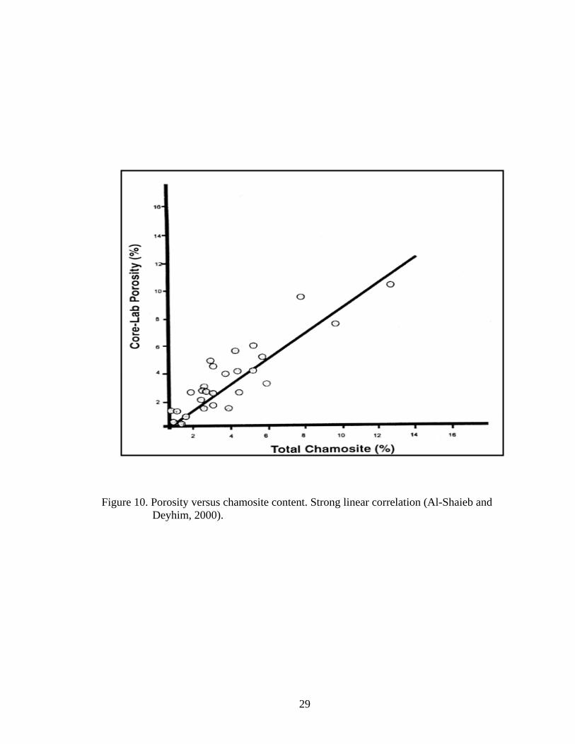
29
Figure 10. Porosity versus chamosite content. Strong linear correlation (Al-Shaieb and Deyhim, 2000).

30
cementation, but most likely before thrusting occurred (Cemen et al., 1995). The second
stage of quartz overgrowths were related to thermal stress (Houseknecht and McGilvery,
1990).
The second phase of diagenesis was the migration of liquid hydrocarbons in both
the west and east. Wells in the eastern portion of the basin contain ubiquitous
pyrobitumen, whereas wells in the west contain only minor amounts of pyrobitumen in
finer grained zones. The presence of pyrobitumen is related to permeability. In the
western part of the basin, as liquids were changed to gas during the heating phase, the gas
cap swept the oil downward though the reservoir except in tight zones. Therefore,
pyrobitumen was left behind as a residue in tight zones. Houseknecht and McGilvery
(1990) state that pyrobitumen residue occurs where the reservoir at the hydrocarbon-
water contact was rendered non-porous by quartz cementation, thus trapping the residue.
In the east where the Spiro sandstones are finer grained and pyrobitumen is pervasive,
overlying seals may have been fractured during the cracking of oil to gas. Some of the
gas in overlying Atokan sandstones may have originated as oil trapped in the Spiro
(Gross et al., 1995).
31
CHAPTER V
Reflection Seismology
This thesis utilized 3D seismic data that has been inverted to acoustic impedance.
Therefore, a brief summary of the theory behind seismic data, seismic acquisition,
processing, and interpretation will be discussed in this chapter. Theory relates to the
different modulii of rocks and how acoustic waves interact with these rocks in the
subsurface. In seismic acquisition, devising parameters to image geologic targets is most
important. Seismic processing takes the raw field data, where the signal is contaminated
with noise and carried on a long unstable waveform, and attempts to create a
representation of the acoustic properties of the earth. Interpretation is the process in
which the geophysicist and geologist tie the earth model from well logs to the seismic.
Seismic imaging is an important tool to help image the subsurface in areas where the
sequence stratigraphy and structure are not well understood and are complicated by
features not observed on the surface. Selective major references on reflection seismology
include Macpherson (2001), Graul (1981), and Wallner (1974).

32
THEORY
Seismic data is produced by sending artificial energy into the earth and recording
its response. This idea was first discovered when large explosives were set off and
recorded by earthquake seismographs (Wallner, 1974). An English seismologist by the
name of Robert Mallet in the mid 1800s was the first to experiment by setting off large
controlled sources of energy and measuring the travel times of the shock waves (Wallner,
1974). Abbot (1878) was the first to measure velocity information from artificial seismic
waves. In 1888, August Schmidt became the first seismologist to propose time-distance
records that would show variations in velocities of seismic waves at depth. However, the
first real use of seismic data for interpreting the subsurface geology was started in the
early 1920s (Wallner, 1974).
In the mid 1920s, Ludger Mintrop was the first to discover a petroleum reservoir
using seismic. He discovered the Orange Salt Dome off the Texas Gulf Coast. His
seismograph was later converted into seismometers, now known as
geophones/hydrophones, that are sensitive electronic recorders and electromagnetic
(Keppner, 1991).
These early geophysicists were using a refraction method to gather information.
Refraction seismic uses shot-detector distances that are much greater than the depth they
are exploring. The refraction method only records the minimum time paths and thus only
records events that are shallow in the subsurface. Reflection uses much smaller shot to

33
detector distances and is able to image formations much deeper in the subsurface. Today
reflection is widely used in exploration seismology (Wallner, 1974).
Seismic energy travels into the ground in a spherical wavefront, similar to
dropping a pebble into a pond. This is explained by Hyguen’s principle which states that
any point on a wave can be considered as a point source for the next wave (Macpherson,
2001). When a wave enters the subsurface, that wave can be reflected, refracted, or
transmitted and converted to different modes. Commonly, only P-waves are recorded, but
when a P-wave is transmitted through the ground there is a mode conversion which also
generates a transmitted S-wave, transmitted P-wave, reflected P-wave and reflected S-
wave.
Embedded in this data is a measure of the physical characteristics of the
subsurface rocks based on their elastic characteristics. The elastic parameters of the rocks
are controlled by Bulk, Shear, and Young’s modulii. The Bulk modulus measures the
compressibility of a material. The Shear Modulus measures how rigid a material is by
measuring the stress to strain ratio. The Young’s modulus measures the stiffness of a
material when opposing forces are applied (Davis and Reynolds, 1996). Fluid type in the
pore space also plays a major role in how the reflected energy responds. Poisson’s ratio
describes how that rock bulges when shortened.
Acoustic impedance is the product of the velocity of the sound waves in rock
times the density of the rock. Acoustic impedance is an important parameter in that it
contains both velocity and density information. The reflection coefficient is defined as
the amplitude of the reflected wave divided by the amplitude of the incident wave.
Reflection coefficients are a function of the acoustic impedance. Acoustic impedance can

34
relate directly to rock type, pore space, pore fluid, and reservoir quality. The reflection
coefficient is dependent upon the contrast of acoustic impedance between two layers. The
reflection coefficient is then
Z2 – Z1
Z2+Z1
Where Rc is the reflection coefficient; Z2 is the acoustic impedance of layer 2 and Z1 is
the acoustic impedance of layer 1 (Macpherson, 2001). For large acoustic contrasts the
stronger the reflection coefficients are in the subsurface the larger the reflection will be
recorded at the surface. The concept of reflection coefficients is illustrated later on in
Figure 12.
ACQUISITION
During surface seismic acquisition, an energy source, for example vibroseis or
dynamite, is used to send sound waves into the ground. Surface detectors record reflected
events from different acoustic boundaries in the subsurface. Acoustic events are defined
by their frequency, amplitude, and time. Seismic frequency usually ranges from 20-80
cycles/second, or hertz. Amplitude is defined as the strength of the reflection coefficient
from a boundary in the subsurface. The higher the reflection coefficient is the higher the
amplitude. Time is the measurement of the downgoing energy reflected from a boundary
and then detected at the surfaces (Wallner, 1974).
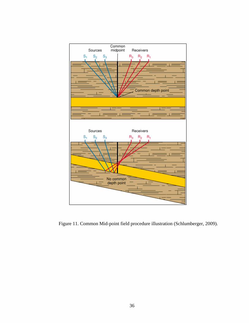
The geophysicist’s knowledge of the subsurface will determine how the field
acquisition of groups and shots is planned. The CDP field procedure is used to give
RC =

35
repeated reflection recordings with varying surface moveout distances of a common
subsurface reflection area (Wallner, 1974) (Figure 11). Gain systems are used in the field
to see the raw data. Decay of amplitude of the seismic signal occurs because of
scattering, spherical divergence, attenuation loss, and amplitude distortion through
frequency loss (Wallner, 1974) (Figure 12).
During seismic acquisition, there are many important factors that need to be
optimized to image the targets of interests. Frequency and amplitude are recorded using a
wide band of frequencies from under 10 to over 100 cycles per second. However, high
and low frequencies are often masked due to wind or shot-hole noises, ground roll and
other coherent and incoherent noise sources which interfere with the reflected signal.
Thus, the bandwidth of the data is usually somewhat narrow and thin beds are hard to
resolve (Wallner, 1974). The type and strength of the source energy will be dependent on
how strong the reflecting events might be. Seismic data is recorded in time and are also
commonly displayed in time. The 3D data used for this thesis project was acquired using
dynamite which gives a broader frequency spectrum than vibroseis, which has difficulty
generating the low frequencies. The higher the bandwidth of frequencies sent into the
ground the higher the resolution, resulting in thinner beds being resolved. Therefore, it is
important to have a wide range of frequencies to get higher resolution data (Wallner,
1974).
36
Figure 11. Common Mid-point field procedure illustration (Schlumberger, 2009).

37
Figure 12. Attenuation losses of the seismic signal (Modified Graul, 1981).
Geologic Layers Acoustic Impedance
Reflection Coefficient
Reflection Coefficient
Reflection Coefficient
Stickogram Stickogram showing transmission losses
Stickogram showing spreading and transmission losses

38
PROCESSING
Seismic processing consists of a multitude of steps that converts raw field data
into a seismic section that can be interpreted to better understand stratigraphy, structural
geology, and oil and gas potential of the area where the data was acquired. Initially raw
field seismic data is edited on a trace by trace basis eliminating bad channels or groups.
Spherical divergence correction is then applied to account for attenuation in the Earth.
First, deconvolution stabilizes the waveform and statics are applied to correct for
near surface velocity anomalies. Normal Moveout (NMO) velocity is the velocity needed
to flatten the traces in a common depth point (CDP) gather so that stacking these traces
will enhance the signal (Figure 13). NMO velocity is found using statistics, and trial and
error (Figure 14). Often the processor will generate semblance plots where they pick the
best velocity to move events back to their right place in time due to large offset distances
so that these CDPs stack properly (Graul, 1981).
Second, migration, a processing technique, is applied to move events to their
proper place. Today migration is commonly done before stacking and is called pre-stack
time migration. Migration seeks to collapse diffraction events to points by moving events
to their proper place in time and space (Gray, 2001). There are two types of migration,
time and depth. Time migration uses an imaging velocity to produce an image that may
not be a correct velocity model for the geology. Depth migration uses an interval velocity
model, which is a model of the Earth’s subsurface (Gray, 2001). Unfortunately, depth
migration requires a lot of velocity estimation leaving room for more error. Therefore,

39
Figure 13. Common Midpoint (CMP or Common Depth Point CDP) NMO correction. Before normal moveout events are not in the right time due to increasing offsets from the CMP. After NMO correction events are moved to the right place in time. (Schlumberger, 2009).

40
Figure 14. Semblance plot on the left showing best velocity picks. On the right is the NMO corrected data (Ikelle and Amundsen, 2005)

41
many geophysicists use time migration. Many different methods of migration exist such
as Kirchoff migration (Figure 15).
Third, stacking, the most powerful processing step, is applied to sum all traces
that contain a common midpoint to equal one trace. Stacking the data eliminates most of
the noise and the redundancy of traces added together to give higher amplitude signals
(Graul, 1981).
The data set for the study area has had an additional post migration step called
inversion which will be discussed in the next chapter.
INTERPRETATION
Well logs have good vertical resolution of the earth, in depth, whereas seismic has good
lateral resolution of the earth, recorded in time. Therefore, to calibrate well data to
seismic, time-depth relationships have to be established to correlate one to the other.
Many seismic interpretation software packages contain time to depth algorithms that can
be applied to well data to convert depth data to time. After a time depth chart has been
created, a geophysicist can generate a synthetic seismic trace. A synthetic seismogram is
made by convolving a wavelet with the reflectivity series from the well. The reflectivity
series consists of all of the reflection coefficients based on the differing acoustic
impedance contrasts between interfaces. A synthetic seismic trace can be created from a
sonic log of a well in the area covered by seismic data to determine how the well logs and
formation tops correlate to the seismic data.

42
Figure 15. Simplistic view of a point diffractor collapsed to a single point using Kirchoff time migration method (Gray, 2001)

43
Knowing the phase of the seismic data is one of the most important pieces of
information to extract from the data. A zero phase wavelet is what most geophysicists
want to work with so that a single peak refers to an impedance increase in normal polarity
(Figure 16). Mixed phase wavelets tend to decrease the quality of the seismic because a
mixed phase wavelet will not image the subsurface correctly (Henry, 1997).
At the interpretation stage, the data has been properly imaged but there is a limit
to the resolution of data due to the lack of temporal resolution (Graul, 1981). When units
are thick, porous and continuous they are easily imaged in seismic. However, with the
recent advances in horizontal drilling technology thin, tight, discontinuous beds can be as
important to oil and gas production as thicker beds, so it is necessary to be able to image
the thin beds as well as the thick beds.
A seismic attribute is simply a measurement derived from seismic data, usually
based on measurements of time, amplitude, frequency, and/ or attenuation (Graul, 1981).
Seismic attributes can be used to relate many quantities such as well productivity to the
seismic data. They have the same common components of arrival time, amplitude,
signature (waveform shape), and a combination of the above (Graul, 1981). Direct
Hydrocarbon Indicators (DHI’s), for example can show up in the seismic data as a
“bright spot,” which is related to the rocks velocity, density and acoustic impedance as a
function of porosity and fluid in the pore space (Wallner, 1974). Polarity reversal can also
be an indicator of hydrocarbons. Also flat spots can be good DHI’s. A fluid contact is
expressed as a flat spot in seismic data (oil on water, or gas on water, or gas on oil) where
there are large contrasts in amplitude from the reflected horizon.

44
Figure 16. Zero phase wavelet (on the right) versus a mixed phase wavelet (on the left) which was only seen when computing a frequency versus phase cross plot. Notice the two side lobes seen in the mixed phase wavelet determined by statistical deconvolution versus the nice strong peak with no side lobes seen in the zero phase wavelet (Henry, 1997).
MIXED PHASE ZERO PHASE

45
Another important seismic attribute is amplitude versus offset (AVO), which is
defined by the normal incidence refection coefficient and the contrast in Poisson’s ratio at
the reflector (Rutherford, 1989). This calculation is done before the CDP data is stacked.
Three classes have been assigned to gas sands based on their AVO characteristics
according to Rutherford. Class 1 gas sands have higher impedance than the encasing
shale with large positive reflection coefficient values. Class 2 gas sands have nearly the
same impedance as the encasing shale and have reflection coefficient values around zero.
Class 3 sands have lower impedance than the encasing shale with negative reflection
coefficient values (Rutherford, 1989). In other words, Class 3 sands are soft and slow
while Class 1 sands are hard and fast. For this case, all show decreasing amplitude with
offset at the top of the gas sand.
Eissa and Castagna (2003) suggested that lower Atoka sandstones show a phase
reversal and therefore are classified as Class 1 sands according to the Rutherford (1989)
classification system (Figure 17). They concluded that AVO analysis can be used in these
high impedance gas sandstones of the Arkoma Basin to locate pore fluids.

46
Figure 17. Phase reversal from a peak to a trough showing a target interval using AVO analysis to identify fluid in pore space (Eissa and Castagna, 2003).

47
Chapter VI
SEISMIC INVERSION
The data set used for this thesis is seismic data that has been inverted to acoustic
impedance. Seismic inversion data differs from conventional reflection seismic in that it
has been processed in a way that the effect of the wavelet has been removed. By
removing the effect of the wavelet, the stratigraphy of the formations is better resolved.
In this thesis, two units which were previously mapped as one unit in the conventional
seismic, were identified independently from each other in the inversion seismic data. This
seismic inversion data has been inverted to acoustic impedance, which relates linearly to
porosity and can be used to map areas of potentially higher porosity. Some of the most
useful resources used in writing this chapter are from Hampson and Russell (1999),
Francis (2006), and personal communication with Gorka Garcia, currently employed by
Odegaard America Inc, who performed the inversion on the data utilized in this thesis.
Seismic inversion was first used in the 1980’s when it was realized that not every
sample in a seismic trace represents a unique reflection coefficient (Pendrel, 2001). In
seismic inversion the goal is to remove the wavelet and return to just the reflection
coefficient series. A well is commonly used to quantify the low frequency part of the
change in impedance with depth so that the acoustic impedance values that result are
actual values for the rocks encountered in the area. This is called absolute acoustic
impedance (Pendrel, 2001). In other words, there is an attempt to recover the acoustic

48
impedance as a function of depth (or time) from observed normal incidence seismograms
(Francis, 2006). Seismic inversion is especially important when studying the stratigraphy
of an area because it removes the effect of the wavelet. Therefore, inversion data can be
used to map thickness changes in rock units as well as to better understand changes in
rock properties.
THEORY
The theory behind inversion involves the most fundamental part of a seismic
section, the seismic trace. A seismic trace can be thought of as having three parts; a
reflectivity series, a wavelet, and noise. Seismic inversion seeks to deconvolve the
seismic by removing the wavelet and leaving just the reflectivity series. The reflectivity
series would be seen as spikes ideally at every bed interface. Reflectivity is calibrated to
acoustic impedance using well control. Since the data is bandlimited the inversion data
traces will still have some width to their traces and will not be seen as a perfect spike at
each interface. However, the resolution of inversion data is much higher allowing for
thinner beds and more bed contacts to be mapped as well as mapping changes in facies
away from well control.
Inversion is used to estimate a model from a set of data and is often non-unique in
the sense that a given data set can be produced by many different models. The
mathematical objective of an inversion algorithm is to minimize the “objective function”
which is a measure of the difference between calculated and observed data. An inversion
algorithm is a coupling of forward modeling and an inversion engine. Forward modeling

49
generates a seismic response by combining the Earth model with a model algorithm.
Inverse modeling simply uses an inverse algorithm to get back to the Earth model
(Banihasan et al., 2006).
There are nine types of inversion discussed in this thesis and they are 1) global
inversion, 2) local search techniques, 3) deterministic, 4) descent type techniques, 5) band
limited, 6) blocky inversion, 7) stochastic, 8) constrained, and 9) sparse spike (Figure 18).
1) Global inversion is for highly non-linear problems and requires a very large number of
trial solutions (Francis, 2006). The global inversion method inverts more than one trace
at a time which will produce a smoother looking inversion by suppressing noise while
maintaining resolution (Pendrel, 2001). 2) Local search techniques is the simple model
which can only be used for moderate non-linear problems and does not require as many
trial and error steps. 3) Deterministic inversion uses well data and seismic to create a
broad bandwidth impedance model of the Earth (Francis, 2006). The inversion data used
for the study area was modeled using a deterministic inversion based on simulated
annealing (Garcia, Odegaard America Inc.). 4) Descent type methods use derivative
information and only require a small number of trial solutions. Two types of descent type
inversion are: 1) Newton type, which requires partial derivatives, is very efficient for
quasi-linear problems used for most types of post-stack seismic inversion, and 2) gradient
based methods, which require only the gradient direction. Inversion comprises three basic
steps: a) converting seismic amplitudes to reflection coefficients: b) converting the
reflection coefficient spikes to acoustic impedance contrasts, which is the actual inversion
step, and c) converting the impedance changes to absolute impedances by the addition of
a low frequency model (Castagna, 2007).

50
Figure 18. A non-specific example of an inversion model where (a) is a three layer Earth model, (b) acoustic impedance, (c) reflection coefficients (d) convolution of reflectivity series with a wavelet. Remove the effect of the wavelet to get back to acoustic impedance (Modified Hampson -Russell, 1999).

51
The sole purpose of the low frequency model is to attain low frequencies from
well log data to attain absolute impedance. As depth increases rocks are more compacted
and thus have increased velocities. The low frequency model expands the bandwidth of
the seismic data thus giving a more accurate interpretation of what is taking place in the
subsurface.
5) Bandlimited inversion method suggests that if a seismic trace represents the
Earth’s reflectivity series, then once that trace is inverted it would become acoustic
impedance (Hampson-Russell, 1999). This method is flawed since the seismic trace is
bandlimited, which means that low and high frequencies are not represented in the
seismic trace. 6) “Blocky Inversion” model uses a series of blocky pseudo velocity logs
resulting in a coarser resolution of the data. The average size of the block is generally
larger than the sample rate of the data. The three pieces of data used are thickness,
density, and velocity of the layer of interest. 7) Stochastic inversion method considers
that the seismic trace and the initial guess impedances are two pieces of data that will be
merged to give the final results. 8) Constrained inversion sets an initial guess as a starting
point for the inversion data and sets absolute boundaries for other parameters that may
deviate from that initial guess. 9) Sparse spike inversion seeks to find a reflectivity series
from the seismic section that contains both high and low frequencies. Sparse Spike
inversion produces two sets of data; a relative and absolute impedance data set, but other
methods such as the deterministic method also produce two sets of data (Pendrel, 2001).
The relative impedance data set has no low frequencies added, whereas the absolute data
set has the low frequency model added. The seismic data used for interpretation in the
52
study area was an absolute impedance data set with the low frequency model added
(Garcia, Odegaard America Inc, 2005).
PROCESS OF INVERSION
There are many different steps to generate seismic inversion data from the time it
is processed to the time it is interpreted (Figure 19). Gorka Garcia, employed by
Odegaard America Inc., performed the inversion in 2005 for the data used in this thesis.
The steps used for the inversion include data quality control, of both the seismic data and
well control, log calibration, wavelet estimation, low frequency model, and finally the
inversion. The first step is studying the quality of the data. This step includes adjusting
sonic and density curves and picked horizons on the seismic data. The second step
includes calibrating the well data to the seismic data by shifting the data up and down in
time to make a good match between the seismic and well data. The third step is wavelet
estimation which is done by extracting a wavelet from the seismic data.
There are three methods that are commonly used to calculate the wavelet that is
imbedded in the data. The first method is “purely deterministic” which would measure
the wavelet directly using surface receivers. The second method is “purely statistical”
which would derive the wavelet from seismic data alone (Hampson-Russell, 1999). This
method is sometimes unreliable because it is sometimes hard to determine the phase
spectrum. The third method is using a well log which would ideally tie perfectly or
almost perfectly to the seismic (Figure 20). The third method may not produce a good
wavelet extraction if the tie is not exact, which results in a poor depth to time conversion.

53
Figure 19. Basic workflow of seismic inversion from processing to interpretation (Garcia, Odegaard American Inc.)

54
Figure 20. Well calibration to extract a constant phase wavelet from the data (Garcia, Odegaard America Inc). Description: Red line on seismic section represents synthetic ties. The sonic log is being edited where a checkshot existed and is colored blue with the original shown in red.
Fu llstack c onstant p hase wavel et extrac ti on (us ing check shot & 72.0 ms bulk s hift)
55
Wavelets can change from trace to trace as a function of time, so the optimum wavelet
extraction method is to find an “average” wavelet for the entire seismic data cube
(Hampson-Russell, 1999). For this study a constant phase wavelet was extracted using
the well log method. A constant phase wavelet is extracted by calculating the amplitude
spectrum from the seismic alone and the phase is assumed to be constant. This type of
wavelet extraction tends to be most robust where there are imperfect well ties (Hampson-
Russell, 1999).
The fourth step is adding the low frequency model to the data. As discussed
earlier in this chapter the low frequency model adds low frequency data, collected from
well data, to the seismic data since surface seismic does not record low frequencies. The
low frequency model increases the bandwidth of the seismic data and thus allows for a
more accurate seismic inversion. After these steps are taken, the seismic data is ready to
be inverted to acoustic impedance using a series of algorithms. When the inversion
process is completed, calculated acoustic impedance curves, from well data, are
compared to the seismic for quality control checks.
SEISMIC ACOUSTIC IMPEDANCE VERSUS WELL LOG ACOUSTIC
IMPEDANCE
Four well logs, calibrated to seismic, were used for the inversion used in this
thesis project. These wells contained sonic, one with a checkshot, and density logs. A
checkshot survey is generated with a receiver located in the borehole at a known depth.

56
After a source has been generated at the surface the time to reach the receiver is recorded
(Schlumberger, 2009). Therefore, the depth and time are known values and can be
compared to a sonic log to adjust the accuracy of the sonic log to the seismic.
The wells used for the inversion were wells 1, 2, 3, and 4. Eventually well 3 was
dropped from the inversion project because of misties. Well 1 and well 4 show similar
velocity and density values. However, well 2 shows much different rock properties and
thus does not make as good of a tie to the data. Therefore, to check how well log values
compared to sonic values, a crossplot of average seismic values and well log values in the
Spiro Sandstone was generated (Figure 21). Averages had to be used because of the
vastly different sample rates and resolutions of seismic data and well log data. The
sample rate of the seismic data is 4ms, approximately every 18 feet, and well logs values
were sampled every 0.5 foot.
Due to the wide range of velocities used for inverting the seismic data, there is a
lack of correlation between calculated acoustic impedance (from well log values) and
seismic acoustic impedance. The lack of correlation between calculated acoustic
impedance and seismic acoustic impedance can be the result of many things. First, the
low frequency model can affect the values of acoustic impedance away from wells that
were used in the inversion process. An example of a well with a poor low frequency
model is shown for well 4 (Figure 22). Low frequencies travel much farther than higher
frequencies and thus are not generated by surface seismic. Therefore, addition of the low
frequency model is important for an accurate inversion. However, the answer to the
problem is probably due to limited data. With only 3 wells and seismic data used for the

57
Figure 21. Chart graphing acoustic impedance from seismic versus calculated acoustic impedance from well log data. Wells 1, 2, 3, and 4 were used in the inversion process.
Calc'dAI vs Seis AI
34000
34500
35000
35500
36000
36500
37000
37500
38000
38500
25000 30000 35000 40000 45000 50000
Calc'd AI
Seis
AI
Well 6Well 1Well 4Well 2Well 8Well 7Well 5

58
Figure 22. Green arrow points to where the low frequency model (blue line) and
log curve values (red line) do not match (Garcia, Odegaard America Inc).
R o c k _ is la n d _ 3 5 - L o w f r e q u e n c y m o d e l , A I

59
inversion, a lot of interpolation was made in between wells. If more wells contained
density logs, and sonic logs this issue may have been better resolved. However, for many
reasons, it is impossible to always have a complete suite of well logs for each well
location. Some examples of where the well log calculated acoustic impedance and
seismic acoustic impedance differ significantly are shown (Figure 23). In general the
seismic data has underestimated the acoustic impedance values compared to the
calculated acoustic impedances generated from log data. However, in lower acoustic
impedance values seen in seismic do, in fact, correlate to lower acoustic impedance
values calculated from well logs.

60
Figure 23. Green circles indicate areas where the seismic acoustic impedance result (blue line) and log curve acoustic impedance (red curve) do not match. This is located at the Spiro Sandstone horizon. (Color scale for seismic inversion is in kg/m2s) (Garcia, Odegaard America Inc.).

61
CHAPTER VII
INTERPRETATION OF THE INVERSION DATA
The Late Morrowan Wapanucka Limestone and the Lower Atokan Spiro
Sandstone are two important gas producing reservoirs in the study area. The two units are
impossible to distinguish on the conventional seismic data. Therefore, in previous studies
Parker, 2007 and Sadeqi, 2007 the two units were analyzed as a package because they
were masked by one large peak (Figure 24). The new inversion data was able to resolve
the two units as separate units because the effect of the wavelet has been removed and the
large impedance contrast between the two units. This large impedance contrast was
between the slower more porous sandstone of the Spiro and the faster less porous
limestone of the Wapanucka Formation. In order to separate the two units a calculated
impedance curve was tied to the seismic as well as a gamma ray log and sonic log (Figure
25). After the logs were tied to the seismic, the picking tool was used to pick the base of
the Spiro/ top of Wapanucka and the base of the Wapanucka. The top of the Spiro was
previously picked using the PSTM (pre-stacked time migrated) data by Parker (2007).
By picking the Spiro Sandstone as a unique unit, amplitude and isochron maps
were generated to map areas of interest. In the study area an area of interest is defined as
an area with greater thickness and lower impedance that relates to higher porosity in the

62
Figure 24. PSTM (pre-stacked time migrated) data resolving the Spiro Sandstone and Wapanucka Limestone as a single reflector in a vertical seismic display in KINGDOM Suite 8.1. Descriptions: The yellow curve is the synthetic trace and the light blue is the gamma ray. The black curves in the background are the seismic traces overlain on the color filled seismic data. The tops and bases of units are marked on the GR curve. On the synthetic the top of the Spiro would is seen as a large peak and the base of the Wapanucka is seen as a large trough.
Base Wapanucka
Top Spiro Sandstone
TopWapanucka

63
Figure 25. Inversion data allowed for the differentiation between the Spiro Sandstone and Wapanucka Limestone shown in a vertical display in KINGDOM Suite 8.1. Descriptions: The pink curve is the acoustic impedance calculate curve, the red curve is the sonic curve, and the dark blue curve is the gamma ray. The display is shown in two wave travel time (TWT). The color bar is in acoustic impedance, 1= largest acoustic impedance value 0= lowest acoustic impedance (kg/m2s).
Base Wapanucka Limestone
Base Spiro/ Top Wapanucka Limestone
Top Spiro Sandstone

64
Spiro Sandstone. Therefore, thickness changes in the Spiro as well as rock property
changes could be attributed solely to the Spiro Sandstone. Sonic logs were analyzed to
check for velocity contrasts. The project contained 11 sonic logs of quality that reached
the Spiro Sandstone. Acoustic impedance was correlated to porosity where porosity logs
existed. Higher porosity caused a decrease in acoustic impedance, since changes in
acoustic impedance are directly related to the rock properties. In cases where the Spiro
Sandstone is more porous, the velocity was slower than where the sandstone was tightly
cemented.
STRUCTURE
Structure plays an important role in controlling the productivity of the Spiro
Sandstone. Impedance changes directly relate to rock property changes, which are
controlled by either structure or stratigraphic changes within the unit. Parker (2007) and
Sadeqi (2007) mapped four different thrust sheets in the footwall of the Choctaw fault
zone within a duplex structure (Figure 26). Four different thrust sheets of the Spiro and
Wapanucka were analyzed in the study area (Spiro/Wap_1, Spiro/Wap_2, Spiro/Wap_3,
and Spiro/Wap_4). Structural changes of the Spiro Sandstone/Wapanucka Limestone
were previously studied over seven seismic cross sections (Parker, 2007 and Sadeqi,
2007). Four lines of cross section were parallel to dip (dip lines) and three lines were
approximately perpendicular to dip (strike lines). The dip lines were most important in
showing rock property changes related to structural control and the strike lines were most
useful in looking at lateral changes.

65
Figure 26. Location of four different thrust sheets of the Spiro/Wapanucka in the study area. Time maps are in ms.
Four different thrust sheets in the study area shown in time maps (ms)
Thrust sheet 1
Thrust sheet 2
Thrust sheet 4
Thrust sheet 3

66
As mentioned earlier, a few rock properties that effect acoustic impedance are
porosity, fluid content, cementation, and facies changes. Arbitrary lines were drawn
across the survey area approximately parallel to dip to illustrate relationships between
structure and acoustic impedance. In areas where the Spiro Sandstone has been tightly
folded in an anticlinal shape, it is possible that increasing porosity may be associated with
an increased fracture density (Figure 27). This is shown in Figure 28 where the highly
folded hanging wall of the thrust fault of the Spiro Sandstone has more porosity than the
broad synclinally shaped footwall of the thrust fault. Horizon contour maps of the top of
Spiro and base of Spiro were made to analyze areas of tighter folding (Figure 29).
Arbitrary lines were drawn through the horizon contour maps to see if the folds
resembled synclinal or anticlinal folding (Figure 30).
The goal of analyzing the structure was to infer where areas of tighter folding
existed in the study area that may contain higher porosities due to fracturing from
compression. Lower impedance values are not necessarily seen in these areas because the
highly folded areas experience imaging problems due to energy dispersion off the tight
structure. However, using inversion seismic data, solely, as a tool for predicting fracture
concentration and stress direction orientation is a broad assumption. Therefore, core data
would have been needed to verify the existence of open fractures where porosity values
are in the inversion data.
All wells with sonic logs were analyzed to see what an average velocity for the
Spiro Sandstone would be and where outliers existed in the survey (Figure 31). Velocity
and acoustic impedance were then crossplotted to show that slower velocities would
correspond to lower acoustic impedances (Figure 32). In areas where wells have

67
Figure 27. Two thrust of the Spiro penetrated in a well that had porosity information. The first Spiro shows a tighter anticlinal type fold. The second Spiro shows a very open syncline. PSTM Data. Color bar is in amplitude units.
1st Spiro thrust penetrated
2nd thrust Spiro penetrated

68
Figure 28. Well 2 crossplot of acoustic impedance versus porosity (density porosity sandstone matrix) showing that the hanging wall (first thrust block) of the Spiro Sandstone has more porosity than the footwall (second thrust block) of the Spiro Sandstone. The first thrust block is in blue and the second thrust block is in pink.
AI (using Faust Velocity) vs. Porosity
0
10000
20000
30000
40000
50000
60000
70000
0 5 10 15 20 25
Porosity
Aco
ustic
Impe
danc
e
Spiro_1Spiro_2
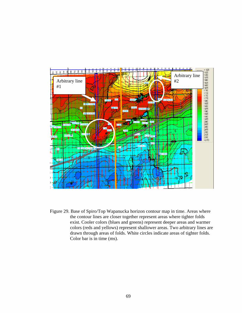
69
Figure 29. Base of Spiro/Top Wapanucka horizon contour map in time. Areas where the contour lines are closer together represent areas where tighter folds exist. Cooler colors (blues and greens) represent deeper areas and warmer colors (reds and yellows) represent shallower areas. Two arbitrary lines are drawn through areas of folds. White circles indicate areas of tighter folds. Color bar is in time (ms).
Arbitrary line #1
Arbitrary line #2

70
Figure 30. Arbitrary lines #1 and #2 showing a tighter #1 anticlinal fold and #2 more open anticlinal fold. The yellow line represents the top of Spiro horizon and the dark blue line is the base of Spiro/Top of Wapanucka horizon. Color scale is in acoustic impedance units (kg/m2s).
#1 #2

71
]
Figure 31. Velocities in the Spiro Sandstone vs. depth for all wells with sonic logs. Two outliers; well 2 and well 5. Both of these wells penetrated Spiro that lie near or on faults. The arrow points to well 2 and well 5.

72
Figure 32. Average acoustic impedance values for the Spiro interval crossplotted against velocity for all wells that had sonic logs available. The acoustic impedance values are higher due to poor resolution since they lie on a fault. An R^2 value for the wells not including the outliers = 0.1224.

73
penetrated Spiro Sandstone that has been faulted, slower velocities are expected as well
as lower acoustic impedance (Figure 33). In cases where structure was thought to control
porosity, crossplots were generated to map acoustic impedance versus porosity for
different thrusts of the Spiro Sandstone. Well 2 contains highly fractured Spiro sandstone
that contains much more porosity than the well 1 which is nearby (Figure 34). Overall
acoustic impedance values did not always correlate with tighter folding. Therefore, using
inversion data as tool to determine fracture content is too ambiguous to use with any
certainty, unless fracture density could be determined from core data or FMI (Formation
MicroImager Schlumberger registered trademark) data.
POROSITY
In the Spiro Sandstone, porosity can range from 2 to 30% (Lumsden et al., 1971).
The amount of porosity is dependent on either diagenetic features or fractures. In areas
where diagenetic features are the reason for an increased porosity, the acoustic
impedance data set does a good job at predicting porosity. Acoustic impedance inversion
data is commonly used in industry to predict facies changes correlating to higher
porosities (Figure 35). Reservoir characterization can be greatly enhanced if areas of
higher porosity are accurately mapped. Rock properties, such as porosity, have a large
impact on the acoustic impedance. An acoustic impedance versus porosity, density
porosity run on a sandstone matrix, crossplot was generated for well 2 which showed a
good linear correlation between porosity and acoustic impedance (Figure 36).

74
Figure 33. Arbitrary line drawn across the survey to illustrate the faulting. PSTM Data.
Well 2 (penetrates fault)

75
Figure 34. A crossplot of porosity (density porosity run on a sandstone matrix) versus acoustic impedance showing the relationship between acoustic impedance and porosity contrasting a well with no fault (dark blue, well 1) to a well that penetrated a fault (pink, well 2) in the Spiro Sandstone.
Well 1 and well 2 AI vs Porosity
0
2
4
6
8
10
26000 31000 36000 41000 46000 51000
Z Impedance (gft/ccs)
Poro
sity
(phi
)
Well 1
Well 2

76
Figure 35. An example of impedance vs. porosity. On the left a crossplot of porosity versus P-impedance with the color scale corresponding to different wells for Cretaceous aged sandstones in Magdalena Valley, Columbia (Calderon and Castagna, 2007). On the right examples from the Danish North Sea (Pedersen-Tatalovic, 2008).Lower acoustic impedance values correlate to higher porosity values.

77
Figure 36. Crossplot of porosity (density porosity run on a sandstone matrix) versus acoustic impedance for well 2. Correlation coefficient is 0.584.
Well 2 Spiro Sandstone Porosity vs. Z y = -0.0012x + 39.19R2 = 0.5864
0
2
4
6
8
10
26000 27000 28000 29000 30000 31000 32000 33000 34000
Z (gft/ccs)
Poro
sity
(phi
)

78
As stated previously, acoustic impedance is the product of velocity and density.
Therefore, sonic and density curves were analyzed looking for changes that could later be
related to acoustic impedance changes. Well 5 shows a significant facies change in the
Spiro Sandstone going from a faster, presumably tightly cemented sandstone to a slower,
presumably more porous sandstone (Figure 37). A map of acoustic impedance values in
the Spiro Sandstone (thrust sheet 2) was created using a volume attribute function in
KINGDOM Suite v. 8.1 (Figure 38). This tool essentially windows from one horizon, for
example top of the Spiro, to the next, for example base of the Spiro, and calculates a root
mean squared (rms) value over the interval. This function then computes a horizon that
then represents the rms value of a unit, for instance the Spiro. This horizon can then be
displayed on the survey map giving a single rms value for each X, Y coordinate location
on the survey map.
Arbitrary lines including wells with sonic logs were analyzed across the survey to
see how well velocity and acoustic impedance correlate (Figures 39 and 40). These lines
depict the structural position of the Spiro Sandstone, which identify the thrust sheet in
which the wells lie, and each wells average velocity (in p-wave slowness). These figures
show how acoustic impedance changes relate to structural position and velocity.
Structural position refers to whether the Spiro Sandstone is located in the hanging wall or
footwall of the fault, anticlinally folded versus synclinally folded, or structurally higher
or lower. These lines showed that there is variation between acoustic impedance values
and structural location of the Spiro Sandstone, but more importantly that there is a greater
correlation between velocity and acoustic impedance. Density values do not vary much in

79
Figure 37. Well 5 sonic curve (DT) and Gamma Ray (GR). Sonic shows a faster (boxed in green, avg. 80 µs/ft) and slower portion (boxed in red, avg. 105 µs/ft) of the Spiro Sandstone which may correlate to a change in facies.
FASTER
Top Spiro
Base Spiro
0API 150API
Top Wapanucka

80
Figure 38. Acoustic impedance map of the Spiro Sandstone thrust sheet 2. Cooler colors (blues and greens) indicate lower acoustic impedance values and warmer colors (reds and yellows) indicate higher acoustic impedance values. Color bar is in acoustic impedance units (kg/m2s).
Well 5

81
Figure 39. Arbitrary line drawn across the western edge of the survey along dip to illustrate acoustic impedance changes. Vertical section of arbitrary line showing wells with velocity information projected onto the line. Description: acoustic impedance value (from seismic), sonic log average for Spiro Sandstone in that well, and thrust sheet (in blue). Color scale is in acoustic impedance units (kg/m2s).
37533, 59.84,1 28550, 56.38,1 34608, 62.8,1 30434, 57.72,2 32195, 55.24,2

82
Figure 40. Arbitrary line across the central part of the survey ~along dip with wells projected onto the line. Vertical section of arbitrary line. Wells with velocity information have been projected onto the line. Description: Well name, acoustic impedance value, sonic log average for Spiro Sandstone in that well, and thrust sheet (in blue). Color bar is in acoustic impedance units (kg/m2s).
Well 2 Well 5 Well 1 Well A Well 637932, 86.36, 2 35489, 79.21, 2 36801, 56.92, 2 34837, 52.15, 2 36521, 57.75, 2

83
the Spiro Sandstone because of the environment of deposition. The Spiro was deposited
as a sheet sand, that is interpreted as being formed by the reworking of
progradational/aggradational barrier islands. This study concludes that the linear
relationship between acoustic impedance and porosity holds true for the Lower Atokan
rocks present in the Arkoma Basin.
THICKNESS
Thickness maps are important in determining the lateral and vertical extent of a
reservoir. Generally, isopach maps are constructed from well log data and lack accuracy
when well control is deficient. However, seismic inversion data constrains the thickness
map even more, thus giving a more accurate interpretation since the inversion data has
the wavelet removed, tops and bases of geological units are better resolved and are not
masked by the wavelet. Thickness maps were generated for the Spiro Sandstone in
different thrust sheets of the Spiro to be used as a way to derive thickness information
from the seismic (Figure 41). A crossplot of seismic thickness versus well log thickness
was created to check the quality of the isochron map (Figure 42). A trend line drawn
through the data points in the crossplot gave a correlation coefficient of 0.7029. The
correlation is good enough between actual well thickness and predicted seismic thickness
to use the isochron map as an interpretation tool to predict Spiro sandstone thickness.
The isochron map was computed using the top of the Spiro to the top of the
Wapanucka. Therefore, this thickness calculation is not only Spiro sandstone, but may

84
Figure 41. Isochron map of the Spiro thrust sheet 2. Cooler colors (blues and greens) represent thinner areas and warmer colors (reds and yellows) represent thicker areas. Color bar is in feet.
96.44
91.38
86.32
81.25
76.2
71.13
66.07
61.01
55.94
54.63
50.88
6 miles
Approximately 50 line *50 lines = 1 section

85
Figure 42. Seismic thickness (from isochron map converted to feet) versus well thickness. R^2= 0.7029 with 26 wells used.
Seis (ft) vs Well (ft) y = 0.7029x + 23.496R2 = 0.7029
50
60
70
80
90
100
110
40 50 60 70 80 90 100 110
Well thickness
Seis
thic
knes
s
Series1Linear (Series1)

86
contain minor amounts (<10ft) of Spiro shale. The Spiro Sandstone reaches thicknesses
as great as 100 feet at maximum. However, wells that drill several thrust sheets
containing the Spiro Sandstone could penetrate over 300 feet of Spiro Sandstone, due to
repetition of the strata.
Thickness maps generated in the Spiro Sandstone showed thickness values
ranging from 50 to 100 feet. The depositional environment of the Spiro Sandstone
controls the minor fluctuations in thickness. As discussed earlier, the Spiro Sandstone
was deposited as a sheet sand derived from the reworking of progradational/aggradational
barrier islands. The inversion data used in this thesis may be better suited for calculating
thickness of sandstone bodies higher in the section, which may show greater fluctuations
in thickness based on their depositional setting. Specifically, the sandstones of interest
would be the Panola, Red Oak, and Brazil.

87
VIII
CONCLUSIONS
Seismic inversion data provides a better understanding of the rock properties in
the subsurface. Unlike conventional reflection seismic data which contains mainly
important structural information, inversion data provides stratigraphic information. The
findings for this thesis can be broken into three different areas based on their relationship
to acoustic impedance; structure, porosity, and thickness.
Structure:
• Areas of tighter anticlinal shaped folds may correlate to lower acoustic
impedance values due to fracture porosity
• Horizon contour maps may provide additional insight as to where areas of
greater compression are occurring possibly causing an increase in fracture
density.
• The absolute value of acoustic impedance was unaffected by structural
position.

88
Porosity:
• It is necessary to analyze core data to determine if open fractures exist. Thin
sections are needed to determine if the porosity preserved is primary or
secondary.
• Acoustic impedance and porosity showed a linear correlation. Higher
porosities were seen in areas with lower acoustic impedance
• In areas where the Spiro Sandstone experienced facies changes the acoustic
impedance value was a good predictor of porosity.
Thickness:
• Inversion data resolved two distinct units that were originally mapped as a
package in seismic: the Spiro Sandstone and the Wapanucka Limestone.
• Isochron maps were produced to predict thickness changes in the Spiro
Sandstone. These maps were checked with well log thicknesses and showed a
correlation of 0.707.
• Acoustic impedance values did not show any correlation to thickness values.
Two areas of interest are pointed out where acoustic impedance values are lower and
thickness values are higher (Figure 43 and 44).

89
Future Work:
• Middle Atokan sandstones higher up in the section (Red Oak and Brazil
Sandstones specifically) should be analyzed as they may also be good
candidates for evaluating using inversion data.
• These sandstones exhibit greater fluctuations in thickness due to depositional
processes. They are also encased in shale, which gives a large impedance
contrast both at the top and base of the unit. Therefore, the top and base of
each unit should be able to be picked with accuracy.
• These sandstones may also give good linear correlation between porosity and
acoustic impedance.

90
Figure 43. Areas of interest are circled in yellow. These areas have high producing wells nearby and show significantly lower acoustic impedance values. These areas correspond to thicker areas on the isochron map. Description: Amplitude map using the RMS function discussed in the paper displayed on a basemap. Lower acoustic impedance values are in blues and greens and higher values are reds and yellows. Color bar is acoustic impedance units (kg/m2s).
6 miles
Approximately 50 line *50 lines = 1 section

91
Approximately 50 line *50 lines = 1 section
Figure 44. Isochron map from the top of the Spiro to the base Spiro/ top Wapanucka. Areas circled in yellow correspond to areas of greater thickness and correspond to areas of lower acoustic impedance seen in Figure 43. The color scale is in feet.
96.44
91.38
86.32
81.25
76.2
71.13
66.07
61.01
55.94
54.63
50.88
6 miles

92
REFERENCES
Abbot, H. L., 1878, On the Velocity of Transmission of Earth Waves, American Journal
of Seismology, v.115, p. 178-184.
Al-Shaieb, Z., and P. Deyhim, 2000, Chamosite: a key mineral for interpretation of the
depositional environment of the Spiro sandstone, in K.S. Johnson, ed., Marine
clastics in the southern Midcontinent, 1997 symposium: OGS Circular 103, p.
157-170.
Andrews, R. D., and Suneson, N. H., 1999, Interpretation of surface and subsurface
gamma-ray profiles, Hartshorne Formation, Arkoma Basin, southeastern
Oklahoma: Oklahoma Geology Notes, V. 59, n.2. (April 1999).
Banihasan, N., Riahi, M. A., Anbaran, M., 2006, Recursive and Sparse Spike Inversion
Methods on Reflection Seismic Data, Institute of Geophysics,
University of Tehran
Blakey, R.C., 2005, Paleogeography and Geologic Evolution of North America,
http://www4.nau.edu/geology/.
Branan, C.B. Jr., 1968, Natural Gas in Arkoma Basin of Oklahoma and Arkansas,
Reprinted and Edited from AAPG Memoir 9, v 2, p. 1616-1635, Petroleum
Geology of the Mid-continent Tulsa Geological Society, Special Publication 3.
Calderon, J.E., and Castagna,J., 2007, Porosity and Lithologic Estimation Using Rock

93
Physics and Multi-Attribute Transforms in Balcon Field, Colombia, The Leading
Edge, v.26, no. 2, p. 142-150.
Castagna, John, 2007, Nautilus USA, Seismic Attributes for Exploration and Reservoir
Characterization.
Cemen, I., Al-Shaieb, Z., Hess, F., Akthar, S., and Feller, R., 1995, Geometry of
Thrusting in the Wilburton Gas Field and Surrounding Areas, Arkoma Basin,
Oklahoma: Implications for Gas Exploration in the Spiro Sandstone Reservoirs,
AAPG Abstracts, p. 84.
Cemen, I., Evans, J., and Sagnak, A., 2001a., Eastern Continuation of the Wilburton
Triangle Zone in the Red Oak Gas-Field Area, Frontal Ouachitas-Arkoma Basin
Transition Zone, Southeastern Oklahoma, Oklahoma Geological Survey, Circular
106, p. 81-94.
Cemen, I., Sagnak, A. and Akthar, S., 2001b., Geometry of the Triangle Zone and
Duplex Structure in the Wilburton Gas Field Area of the Arkoma Basin,
Southeastern Oklahoma, Oklahoma Geological Society, Circular 104, p. 87-98.
Cemen. I., Al-Shaieb, Z.., Evans, J., Ronk, J., Syed, M., Sagnak, A., and McPhaill, K.,
2002, Structural Traps along the Frontal Ouachitas-Arkoma Basin Transition
Zone Southeastern Oklahoma, AAPG abstracts, v. 2002, p. 28-29.
Collins, Marline, 2006, Geometry of Late Paleozoic Thrusting, Wilburton and Damon
Quadrangles, Arkoma Basin, Southeast Oklahoma, M.S. Thesis, Oklahoma State
University, Stillwater, OK.
Davis, G.H., and Reynolds, S.J., 1996, Structural Geology of Rocks and Regions, Second
Edition, John Wiley and Sons, Inc.

94
Eissa, M.A. and Castagna, J.P., 2003, Case Study: AVO Analysis in a High-Impedance
Atoka Sandstone (Pennsylvanian), North Arkoma Basin, McIntosh County,
Oklahoma, The Leading Edge, October 2003.
Feenstra,R. and Wickham,J.,1975, Evolution of folds around Broken Bow Uplift,
Ouachita Mountains, southeastern Oklahoma, AAPG Bulletin, June 1975, v. 59,
no. 6, p.974-985.
Francis, Ashley, 2006, Nautilus USA, A Practical Guide to Inversion and Stochastic
Modeling, Earthworks Environment and Resources Ltd.
Fritz, R.D., and Hooker, E.O., 1994, Stop 10, Spiro Sandstone, Oklahoma Geological
Survey, Guidebook 29, Geology and Resources of the Eastern Ouachita
Mountains Frontal Belt and Southeastern Arkoma Basin Oklahoma.
Galloway, W.E., and Hobday, D.K., 1983, Terrigeneous Clastic Depositional Systems:
Applications to Fossil Fuels and Groundwater Resources, 2nd ed, New York.
Garcia, Gorka, Odegaard America Inc., Personal Communication
Graul, M., 1981, Basic Chevron School,GeoQuest International, Inc.
Gray, S.H., Etgen, J., Dellinger, J., and Whitmore, D., 2001, Seismic Migration Problems
and Solutions, Geophysics, September-October 2001, v. 66, no.5, p. 1622-1640.
Gross, J.R., Thompson, S.A., Claxton, B.L., and Carr, M.B., 1995, Reservoir Distribution
and Exploration Potential of the Spiro Sandstone in the Choctaw Trend, Arkoma
Basin, Oklahoma and Arkansas; AAPG Bulletin v. 79, issue 2, p.159-185.
Ham, W.E., 1969, Regional Geology of Arbuckle Mountains, Oklahoma, Oklahoma
Geological Survey, Guide Book 17, p.5-28.
Hampson and Russell Software Services Ltd., 1999, STRATA.

95
Henry, S.G., 1997, Zero Phase can Aid Interpretation, AAPG Explorer.
Hess, F.B., and Cleaves, A.W., 1995, Depositional Environment of the Spiro Sandstone
in the Wilburton, Red Oak, and Kinta Fields, Arkoma Basin, Oklahoma, GSA
Abstracts with Programs, North-Central/South Central Sections, p. 58.
Houseknecht, D.W. and Kacena, 1983, Tectonic-Sedimentary Evolution of the Arkoma
Basin and Guidebook to Deltaic Facies, Hartshorne Sandstone, Houseknecht,
and others, SEPM Mid-Continent section, Volume 1, October 1983- Tectonic and
Sedimentary Evolution of the Arkoma Basin.
Houseknecht, D.W. and McGilvery, T.A., 1990, Red Oak Field, Structural Traps II,
Traps Associated with Tectonic: AAPG Treatise Petroleum Geology, Atlas of Oil
and Gas Fields, p. 201-225.
IHS, 2008, February, http://energy.ihs.com/.
Ikelle, L. and Amundsen, L., 2005, Introduction to Petroleum Seismology, Society of
Exploration Geophysicists, Tulsa, Oklahoma.
Johnson, K.S., 1988, General Geologic Framework of the Field-Trip Area, in Johnson,
K.S. ed., Shelf to Basin Geology and Resources of Pennsylvanian Strata in the
Arkoma Basin and Frontal Ouachita Mountains.
Keppner, G., 1991, Ludger Mintrop, Geophysics: The Leading Edge of Exploration,
p.21- 28.
Koinm, D. N., and Dickey, P.A., 1967, Growth Faulting in McAlester Basin of
Oklahoma, AAPG Bulletin, v.51, no. 4, p. 710-718
Lumsden, D.N., Pittman, E.D., and Buchanan, R.S., 1971, Sedimentation and Petrology
of Spiro and Foster Sands (Pennsylvanian), McAlester Basin, Oklahoma; AAPG

96
Bulletin 55, p.254-266
Macpherson, D.S., 2001, Seismic Fundamentals.
Mahaffie, M.J., 1994, Reservoir Classification for the Turbidite Intervals at the Mars
Discovery, Mississippi Canyon 807, Gulf of Mexico, in P. Weimer, A.H Bouma,
And B.F. Perkins eds., Submarine Fans and Turbidite Systems: GCS-SEPM
Foundation 15th Annual Research Conference, p. 233-244
Parker, W.F.Jr., 2007, Structural Interpretation of Paleozoic Strata as part of
the Transition Zone in the Wilburton Gas Field Using 3D Seismic, Hartshorne,
Higgins, Adamson and Gowen Quadrangles, Southeastern Oklahoma, Arkoma
Basin, M.S. Thesis, Oklahoma State University, Stillwater, OK.
Pedersen-Tatalovic, R., Uldall, A., and Jacobsen, N.L., 2008, Event-based Low
frequency Impedance Modeling Using Well Logs and Seismic Attributes, The
Leading Edge.
Pendrel, J., 2001, Seismic Inversion- The Best Tool For Reservoir Characterization,
Jason Geosystems Canada
Pittman, E.D., and Lumsden, D.N., 1968, Relationship Between Chlorite Coatings on
Quartz Grains and Porosity, Spiro Sand, Oklahoma, Journal of Sedimentary
Research, v.38, no. 2, p.668-670.
Sadeqi, A.W., 2007, Structural Geometry of the Late Paleozoic Thrusting in the
Hartshorne, Higgins, Adamson, and Gowen Quadrangles, Southeastern
Oklahoma, M.S. Thesis, Oklahoma State University, Stillwater, OK.

97
Sahai, S., Cemen, I., and Cox, D., 2007, Application of Seismic Attributes for Enhanced
Structural Interpretation of the Wilburton Gas Field Area in the Southeastern
Oklahoma, AAPG Annual Meeting, Abstracts.
Schlumberger Limited, 2009, http://www.slb.com/
Suneson, N.H., and Hemish, L.A., 1994. Geology and Resources of the Eastern Ouachita
Mountains Frontal Belt and Southeastern Arkoma Basin: Oklahoma.
Oklahoma Geological Survey, Guidebook 29, p. 3.
Suneson, N. H., Cemen, I., Kerr, D., Roberts, M.l., Slatt, R. Stone, C., 2005,
Stratigraphic and Structural Evolution of the Ouachita Mountains and Arkoma
Basin, Southeastern Oklahoma and Western Arkansas: Applications to Petroleum
Exploration, Geological Survey, Guidebook 34, p. 1-4.
Sutherland, P.K., 1988, Late Mississippian and Pennsylvanian Depositional History in
the Arkoma Basin area, Oklahoma and Arkansas; GSA Bulletin, v. 100 no.11,
p.1787-1802.
Rutherford, S. R. and Robert H. Williams, 1989, Amplitude-Versus-Offset Variations
in Gas Sands, Geophysics, v.54, no.6, p.680-688.
Tilford, M.J., 1990, Geological Review of the Ouachita Mountains Thrust Belt Play
Western Arkoma Basin, Oklahoma, Special Publication-Oklahoma Geological
Survey, p. 169-196.
Tulsa Geological Society, 1961, Symposium on the Arkoma basin: Tulsa Geol. Soc.
Digest, v. 29, 152 p. 718.

98
Van Wagoner, J.C., Mitchum, R.M., Campion, K.M., and Rahmanian, V.D., 1990,
Siliciclastic Sequence Stratigraphy in Well Logs, Cores, and Outcrops: AAPG
Methods in Exploration Series 7, p. 55.
Vedros, S. and Visher, G.S., 1978, The Red Oak Sandstone, a Hydrocarbon-Producing
Submarine Fan Deposit, Sedimentation in Canyons, Fans, and Trenches, p. 292
307.
Wallner, J. D., 1974, Applied Petroleum Geophysics, Tenneco Oil.

VITA
Christine Robin Hager
Candidate for the Degree of
Master of Science Thesis: SEISMIC INTERPRETATION OF PENNSYLVANIAN ATOKAN STRATA
USING 3D SEISMIC INVERSION DATA, WILBURTON GAS FIELD, ARKOMA BASIN, SOUTHEASTERN OKLAHOMA
Major Field: GEOLOGY Biographical:
Education: Completed the requirements for a Bachelor of Science in Geology at Oklahoma State University, Stillwater, Oklahoma in December, 2007. Completed the requirements for a Master of Science in Geology at Oklahoma State University, Stillwater, Oklahoma in May, 2009 Experience: Teaching Assistant T. Boone Pickens School of Geology;
Internship: ExxonMobil. Professional Memberships: American Association of Petroleum Geologist,
Society of Exploration Geophysicists, American Geophysical Union, Oklahoma City Geological Society.

ADVISER’S APPROVAL: Dr. Ibrahim Cemen
Name: Christine Robin Hager Date of Degree: May, 2009 Institution: Oklahoma State University Location: Stillwater, Oklahoma Title of Study: SEISMIC INTERPRETATOIN OF PENNSYLVANIAN ATOKAN
STRATA USING 3D SEISMIC INVERSION DATA, WILBURTON GAS FIELD, ARKOMA BASIN, SOUTHEASTERN OKLHAOMA
Pages in Study: 98 Candidate for the Degree of Master of Science
Major Field: Geology Scope and Method of Study:
The Arkoma Basin is a very prolific foreland basin that is actively being explored and drilled today. The structure and depositional setting of the Spiro Sandstone plays a major role in the productivity. Seismic inversion data provides a direct correlation to rock properties and can be used to aid in better reservoir characterization. This study will investigate whether seismic inversion data can be used as a crucial piece of data that can be as influential as well logs in determining areas to drill in the Arkoma Basin. Where well log and core data are limited, this study could provide vital information on what the projected porosity would be in the Spiro Sandstone in a specific structural position. Correlating acoustic impedance values to porosity will lead to more efficient drilling. Findings and Conclusions:
The findings for this thesis can be broken into three different areas based on the relationship to acoustic impedance; structure, porosity, and thickness. Structure: Areas of tighter anticlinal shaped folds may correlate to lower acoustic impedance values due to fracture porosity. Horizon contour maps provided additional insight as to where areas of greater compression are occurring, which may cause an increase in fracture density. The absolute value of acoustic impedance was unaffected by structural position. Core analysis is necessary to determine if open fractures exist as well as thin sections to determine if the porosity preserved is primary or secondary. Porosity: Acoustic impedance and porosity showed a good linear correlation. Higher porosities were seen in areas of lower acoustic impedance. In areas where the Spiro Sandstone experienced facies changes, the acoustic impedance value was a good predictor of porosity. Thickness: Inversion data resolved two distinct units that were originally mapped as a package in seismic; Spiro Sandstone and Wapanucka Limestone. Isochron maps were produced to predict thickness changes in the Spiro Sandstone. These maps were checked with well log thicknesses and showed a correlation of 0.707. Acoustic impedance values did not show any correlation to thickness values.