Sándor Süle: Seismic Methods III, Lab Exercises 1

Seismic lab exercises

SEISMIC LAB 1st Exercise

This type of analysis involves taking either seismic or geologic cross-sections and building a chronostratigraphic chart. Chronostratigraphic charts, also called Wheeler diagrams after the geologist who initially formalized this time-stratigraphy concept in 1958, display both the horizontal distribution of the component sedimentary layers of a sequence but also the significant hiatuses in sedimentation. This diagram is derived from sedimentary successions and is used to show the time relationships of both the depositional systems and system tracts, and their relationship to surfaces of non-deposition (Emery et. al, 1996).

The basic units of the charts are "chronosomes", horizontal ribbons that represent sedimentary rock units bounded by time planes. Chronostratigraphic charts are best constructed from interpreted seismic sections and help understand how sedimentary sections develop through time. The horizontal axis of the chart matches the horizontal dimension of the seismic section and vertical axis represents time (see and work on Figure Lab-1. You can follow the basic concept which I handed over to you in “Seismic Methods II” hand-out on page 13-16). I have already helped you with Figure Lab-2, where the oldest layer is reconstructed already and you have to apply the basic concepts to the overlying layers only.

Exercise to construct a chronostratigraphic chart:

The following section describes how to construct a chronostratigraphic chart. Steps for extracting information from a seismic section to build a chronostratigraphic chart:

1. Carefully interpret the pseudo-seismic section by identifying and marking where reflector terminations intersect seismic surfaces. Identify the type of reflector terminations (onlap, downlap, toplap, and/or truncation).

2. Transfer the numbered reflectors to a time-scale:

a. The horizontal line matches the length of the pseudo seismic section or distance, with SP refering to "Shot Points" numbered 10 through 240. The vertical axis on the lower part of the diagram represents an arbitrary time line.

Sándor Süle: Seismic Methods III, Lab Exercises 2

The numbered time intervals, 1 through 30, are assumed to be of equal duration. b. Transfer the horizontal dimension of the interpreted reflectors, starting with oldest (numbered here as 1), to the bottom of the time chart. Draw this to match the horizontal length of the equivalent reflector. Continue this process in order of deposition for all remaining reflectors, as in the presented movie.

References Emery, D., Myers, K. J., Sequence Stratigraphy, 1996, published by Blackwell Science Ltd., p. 297.

University of South Columbia Sequence Stratigraphy Web page

Wheeler, H.E. 1958. Time stratigraphy. American Association of Petroleum Geologists, Bulletin, v. 42, p. 1047-1063.

Sándor Süle: Seismic Methods III, Lab Exercises 3

Fig Lab-1 EXERCISE 1: CHRONOSTRATIGRAPHIC CHART CONSTRUCTION Create a Chronostratigraphic Chart identifying the following on this Chart: Lithology, Reflection Terminations including "Onlap", "Offlap", and "Downlap". If you have color pencils, it is a little bit easier.

Sándor Süle: Seismic Methods III, Lab Exercises 4

Figure Lab-2 ⁄for the 1st Exercise ⁄

I try to help you with this figure to work on Figure Lab-1. The oldest layer is reconstructed already and you have to apply the basic concepts to the overlying

layers only.

Sándor Süle: Seismic Methods III, Lab Exercises 5

2nd Exercise

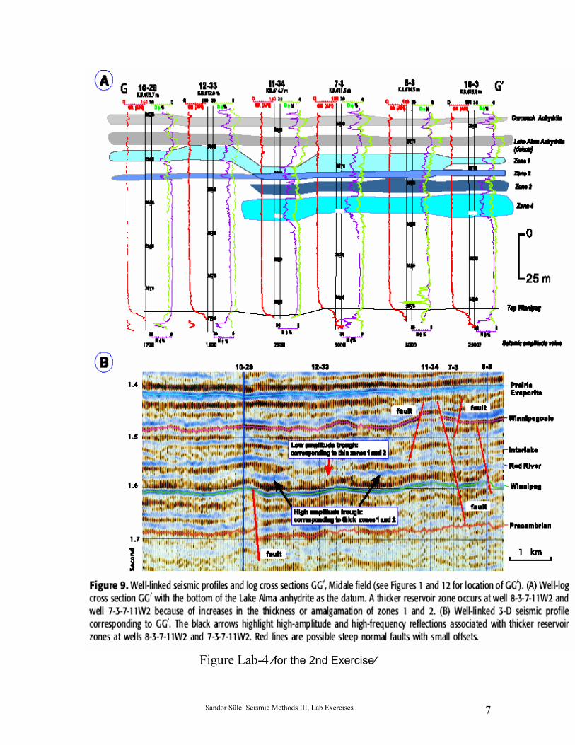
The two figures below are from a volume of the AAPG Bulletin published last year. The title is ‘Pool characterization of Ordovician Midale field: Implication for Red River play in northern Williston basin, southeastern Saskatchewan, Canada’. Wells 7-3(-11W2) and 11-34(W2) are shown on both figures. But there is a contradiction between the interpreted Precambrian horizon (lowest horizon marked with red color). In this depth range the maximum misfit between the interpreted horizon in time and the marker in depth can be a maximum 5 meters. Try to estimate the depth difference between the two differently interpreted Precambrian horizons. Hint:

- between the Winnipeg-Precambrian interval the layers are mainly carbonates (by the 22th page of the handout you can calculate with velocity about 3500 m/s )

- on page 23 of the hand-out you can find a relation to layer thickness calculation from the two way running time and the interval velocity.

Comment: do not be mislead by the synthetic seismogram, this is not important to answer the question. I will speak about the synthetic seismograms in the Friday class.

References L.F. Brown, Jr., J. M. Benson, G. J. Brink, S. Doherty, A. Jollands, E. H. A. Jungslager, J. H. G. Keenan, A. Muntingh, and N. J. S. van Wyk, 1996, Sequence Stratigraphy in Offshore South African Divergent Basins: An Atlas on Exploration for Cretaceous Lowstand Traps by Soekor (Pty) Ltd, AAPG Studies in Geology #41, ISBN#0-89181-049-8, 184 page

University of South Columbia Sequence Stratigraphy Web page

Sándor Süle: Seismic Methods III, Lab Exercises 6

Figure Lab-3 ⁄for the 2nd Exercise⁄

Sándor Süle: Seismic Methods III, Lab Exercises 7

Figure Lab-4 ⁄for the 2nd Exercise⁄

Sándor Süle: Seismic Methods III, Lab Exercises 8

3rd Exercise

The seismic line used in this exercise is a copy of Figure 39 from page 49 of the AAPG Atlas of the “Sequence Stratigraphy in Offshore South African Divergent Basins”. This figure was chosen because it contains clear and easy to interpret examples of onlapping and downlapping sequence geometries and a relatively uncomplicated structural fabric.

The Atlas that the figure comes from has many other similar examples and was initially interpreted by Soekor (Pty) Ltd during their exploration for Cretaceous lowstand traps in the offshore of South Africa.

The upper part of the section is a siliciclastic environment. Try to apply the basic concept of the reflection patterns, written in the handout on page 9-11 and draw the patterns on a similar way with arrows. The lower part is manly faulted carbonated rocks, you can try to find similar faulted features that were presented on the Italian Po-Plain section, given in the Seismic Methods II class. It depends on the person whether he or she likes to start the interpretation with the faults, or with the horizons. I always start with the faults.

Sándor Süle: Seismic Methods III, Lab Exercises 9

Sándor Süle: Seismic Methods III, Lab Exercises 10

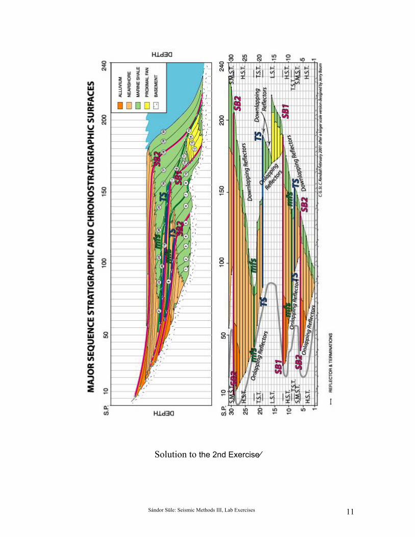
Solutions 1st Exercise The reconstructed chronostratigraphic chart looks like this (next page): As an other example I also attached Peter Vail’s procedure for constructing regional chart of cycles of relative changes of sea level. 2nd Exercise On Figure Lab-4 the two-way-time of the Precambrian horizon at well 7-3 is about 1.68 seconds. On Figure Lab-5 the two-way-time of the Precambrian horizon at well 7-3 is about 1.63 seconds. As the thickness of the layer is given by the one way running time in the given interval multiplied by the velocity:

ondmeterond

sec3500*sec

1005*

21 ≈ 90 meter

3rd Exercise I attached the interpreted section.

Sándor Süle: Seismic Methods III, Lab Exercises 11

Solution to the 2nd Exercise⁄

Sándor Süle: Seismic Methods III, Lab Exercises 12