Seismic travel times and event location

B.L.N. Kennett Research School of Earth Sciences, The Australian National University

• Both the location and nature of events need to be determined

• Locating event hypocentres in space and time requires – a model for seismic wave propagation – means of handling multiple observations

• The interplay between improved knowledge of the

Earth and event locations has played an important role in the development of Seismology

2

Source Characterization

• Hypocentre location employs – arrival times of seismic phases – a representation of the time of passage for the

various phases • It is possible to determine the epicentre by

geometric means, e.g., bracketing using the great circle arcs midway between station pairs in arrival order.

• Depth estimation needs an earth model or travel-time tables.

• All methods depend on some broad idea of the likely location.

3

Event location

• As early as 1911 Geiger was employing least-squares optimisation to determine hypocentres working from an initial trial

• In the 1930’s Jeffreys developed the method of uniform reduction to overcome problems associated with large errors, by reshaping the residual distribution to be closer to the Gaussian assumed in the least-squares technique

• These methods depend on a good starting point and require calculation of derivatives

4

Early Location algorithms

• Representations of the time of passage of seismic phases were needed and these were commonly derived by interpolation in travel-time tables

• Jeffreys started developing tables, and was later joined by Bullen with publication in 1940 of a comprehensive set of tables – these tables relied on assembling information for

different distance ranges from multiple geographic areas where good data was available

– incidentally helped to create the field of “robust statistics”

5

Travel-Time tables

• The J-B tables are very effective, but not wholly compatible between P and S, and depths from P and pP-P differ.

• Baseline issues were clear from known locations of nuclear tests

• In 1987 IASPEI initiated an effort to improve on the J-B tables. An important decision was to use a radial Earth model as a summary of the travel times exploiting the clever representation of tau-splines (Buland & Chapman 1983) to allow rapid delivery of times for multiple phases

6

From tables to models I

• The international effort produced a parametric model iasp91 with a parametric representation of radial structure.

• With relocation of many events to produce a new set of empirical travel times, a further model ak135 was produced in 1995.

• Both models share a simple upper mantle model and reflect the structure encountered between sources and stations – thus a comprise between subduction zone and continental structure

• Compatibility between P and pP is good, so depth phases can be directly incorporated 7

From tables to models II

Radial seismological models

The shaded zones indicate the strongest 3-D variations where a radial 1-D model will inevitably have major limitations

8

Reference models such as ak135 provide a good representation of the times of passage of seismic waves from seismic sources Significant deviations appear out to 30 deg – associated with strong 3-D structure The interruption for S is the crossing of the core phase SKS

9

• The availability of rapid travel-time calculations allows for fully nonlinear algorithms that do not employ derivatives

• An effective procedure is the Neighbourhood Algorithm: the shakeNA program of Sambridge & Kennett (2001), which exploits the properties of the 4-D hypocentral space to seek the best-fitting solutions for some prescribed misfit function (L1 or L2)

• Only a broad initial domain is needed: +/- 2 deg in latitude and longitude, +/- 60 km in depth (where possible), +/- 20 s in origin time

• Good locations can be obtained rapidly with 30 iterations of the NA inversion scheme, i.e., 279 locations tested with 9 new trials per iteration into the best 2 voronoi cells

10

Nonlinear location I

Location Procedure II

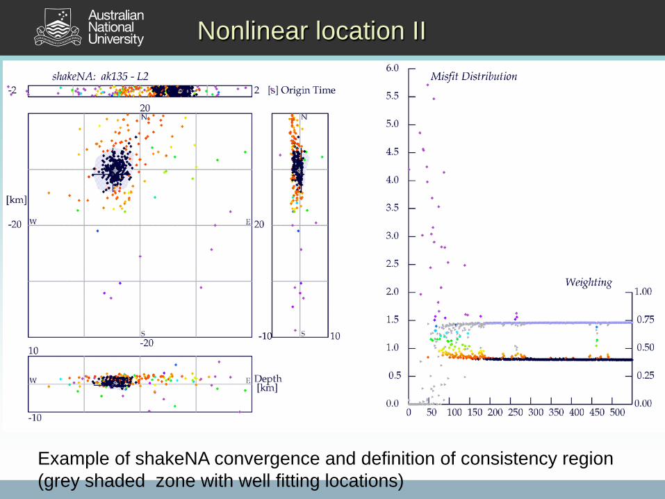
Example of shakeNA convergence and definition of consistency region (grey shaded zone with well fitting locations)

Nonlinear location II

• Such NA procedures work well to extract depth information and converge fast

• Error bounds can be extracted by setting an acceptable level of fit – the consistency region shown in grey in the example

• Alternatively a least-squares procedure can be started from the “best” location to yield conventional error ellipses

• Developments of these ideas underpin the current location methods used at the ISC

12

Nonlinear location III

• How do we explain the success of location with radial models for a 3D Earth? – smoothly varying travel times – heterogeneity averages out – limitation to avoid very large residuals (even

when real) • When using 3-D models

– keep smooth – represent major variations well – block tomographic models rarely suitable

13

1-D vs 3-D models

14

3-D effects - Australia

• Large variation in travel times with west and centre very fast • Locations without allowance for 3-D show large bias • AuSREM 3-D model available

S residuals have similar pattern, but residuals are 3-4 times larger!

15

Residuals after 3-D location

• Location in 3-D AusREM model using nonlinear NA algorithm, with times calculated using Fast-Marching-Method • Comparison of residuals after location in 3-D model and with ak135

• Most systematic effects suppressed or eliminated

16

Hidden 3-D effects

Magnitude dependent locations As the size of event changes different stations are used and influence of 3-D effects becomes important. For event in Flores – as magnitude diminishes location moves away from Australia because dominated by fast paths to WA stations

Billings et al., BSSA 1994

• The earthquake database contains a vast amount of information on the patterns of event residuals

• Needs to be exploited so that multiple large “master” events can be used to recognise arrival patterns to be applied to smaller events, and remove magnitude biases

• Schema: – Preliminary location – Refinement using arrival patterns from data base

Database mining I

18

Database mining II

Raw Residuals from ak135 model for WRA

Smoothed Empirical travel times for WRA

Exploit structure in the data base to recognise multi-scale variations associated with event locations, can represent behaviour more succinctly than a 3-D model. Once event location known approximately behaviour in its neighbourhood can be exploited to refine location.

Figure from: Nicholson, Sambridge & Gudmundsson, GJI, 2004

19

Database mining III

ak135

ETT

The effectiveness of such 3-D oriented Empirical travel times (ETT) is indicated by the reduction in the spread of residuals relative to those for ak135. Need to think of event location as a collective process not just an isolated set of data.

Figure from: Nicholson et al. GJI, 2004