selected paper prepared for presentation at the 2016...
TRANSCRIPT

1
Role of Weather on Design of a Water Quality Trading Program Baseline: A Case Study of
the Jordan Lake Watershed, North Carolina
Marzieh Motallebi
Assistant Professor, Baruch Institute of Coastal Ecology and Forest Science
Clemson University. Georgetown, SC
Ali Tasdighi
Ph.D. Candidate, Department of Civil and Environmental Engineering
Colorado State University, Fort Collins, CO
Dana L. Hoag
Professor, Department of Agricultural and Resource Economics
Colorado State University, Fort Collins, CO
Mazdak Arabi
Associate Professor, Department of Civil and Environmental Engineering
Colorado State University, Fort Collins, CO
Selected Paper prepared for Presentation at the 2016 Agricultural & Applied Economics
Association Annual Meeting, Boston, Massachusetts, July 31–August 2.
Copyright 2016 by Marzieh Motallebi, Ali Tasdighi, Dana Hoag, and Mazdak Arabi. All rights reserved. Readers may make verbatim copies of this document for non-commercial purposes by any means, provided that this copyright notice appears on all such copies.

2
Role of Weather on Design of a Water Quality Trading Program Baseline: A Case Study of the Jordan Lake Watershed, North Carolina
Abstract
Water quality trading (WQT) has been suggested as a cost effective approach to achieve water
quality goals for many watersheds (EPA, 2007), including the Jordan Lake watershed in North
Carolina. Although, theory supports the concept, its implementation has experienced a numbers of
failures in the United States. A broad spectrum of physical, social, economic, and intuitional
factors have diverted success. One of the institutional hindrances is the WQT baseline. WQT
baseline is a reference point that must be met by credit sellers and buyers before being allowed to
buy or sell credits. Favorable (unfavorable) weather compared to the baseline can result in gains
(losses) attributed to conservation technology. We construct a WQT market applied to the new
Jordan Lake Watershed program in North Carolina to examine the role of weather on baseline
period as related to total nitrogen (TN) loads in Jordan Lake. Results of our models show that the
baseline weather condition has a profound impact on the water quality credits supply. The purpose
of this study is to alert policy makers to this issue and to suggest ways to better match the baseline
incentives with emission reduction goals when taking weather variability and trends into account.
Keywords: Water Quality Trading, Baseline, Riparian Buffers, Weather, Jordan Lake

3
Introduction
There have been increasing calls to establish water quality trading (WQT) markets for nutrients
(EPA, 2001, 2004; Willamette Partnership, et al., 2015). Nutrients are the primary culprit in many
of the impaired or threatened lakes, reservoirs, and ponds in the United States (Selman et al. 2009)
and are a seemingly suitable candidate for trading. In theory, water quality can be improved at a
lower cost using WQT than command and control policies such as regulation, which was
successfully demonstrated for mitigating Sulfur Dioxide emission into the atmosphere (Stavins,
2005). The U.S. Environmental Protection Agency estimated that allowing trading between point
sources (PSs) and nonpoint sources (NPSs) could reduce the cost of implementing water quality
goals nationally by $140-235 million annually (EPA, 2001). The conservation measures used to
produce nonpoint source credits can also result in co-benefits, such as improved wildlife habitat
(Lentz et al., 2014).
Conceptually, WQT programs allow polluters with high abatement costs to purchase
credits from firms with lower abatement costs to meet their own regulatory limits. For example, a
waste treatment plant might find it less costly to pay a farmer to install conservation practices to
abate a pollutant, such as nitrogen, than to upgrade their own systems. Although WQT is
conceptually appealing, programs that have been implemented thus far have struggled to show a
meaningful success (Greenhalgh and Selman, 2012; Ribaudo and Gottlieb, 2011; Stepheson and
Shabman, 2010), with only a few trades occurring in any of the programs. A growing list of reasons
why these programs have not found more success have been identified in economic literature,
including high transaction costs, high trading ratios, and trust or uncertainty on the part of buyers
and sellers (Breetz, et al., 2004; Ribaudo, 2013; Newburn and Woodward, 2011; Stepheson and
Shabman, 2010).

4
One of those hurdles is a baseline requirement, which establishes a threshold that must be
exceeded before credits can be offered to others (Ribaudo, 2013). While there is a vast body of
research showing that weather can have a significant effect on the level of pollutant loads to water
bodies (Kang, et al. 2009; Lang, et al. 2013), there has been little attention paid to how this
variation might affect the efficacy of baselines. Therefore, in this study, we determine how weather
congruity between the baseline and implementation date in a water quality trading program effects
the number of credits traded and the impact on cost savings and abatement. Typically, the amount
of pollution in a baseline is dependent on some weather scenario, and many other factors such as
soil types, conservation practice and distance to water. Both point sources and nonpoint sources
are regulated by Total Maximum Daily Load (TMDL) limits, which establishes a cap for an
impaired watershed. Typically, PSs are obliged to adhere to those limits and NPs, like agriculture,
are not. While we found a number of studies that detailed limitations stemming from the way
baselines are established and implemented, we found only one that discussed temporal distortions
in detail related to how pollution is measured between the baseline and point of implementation
(Michaelowa, 2009). The point of that study was to illustrate difficulties related to estimating
pollution across large regions where countries are trading greenhouse gas emissions through Joint
Implementation programs. In the case of Nutrients, data and models are available to make more
precise forecasts, which hides a problem that has not been previously examined. Of course, many
of the problems already discussed in the literature will persist, but none have focused on the
distortion that can be created by rules related to how the weather pattern is chosen by baseline and
implementation decisions.
We build a supply and demand model for an active WQT program in the Jordan Lake
Watershed, North Carolina. Then we isolate the impact of weather on a farmer’s ability to supply

5
credits. We show that if the weather conditions for the baseline were severe, leading to a lot of
pollution, a farmer has a weather advantage toward supplying credits, and vice versa, which either
leads to a lack of additionality in preventing pollution or in raising the cost of the program,
respectively. Using our market model, we then estimate these distortions, and finally we examine
how to improve assumptions about the weather to reduce distortions.
Methodology
A detailed description and study about how baselines affect farmer’s willingness to install
conservation practices and to supply nutrient credits can be found in Ribaudo, Savage and
Talberth, 2014. They establish no lose (Millard-Ball, 2013) baselines that act as eligibility
requirements (Horowitz and Just, 2013) that farmers must achieve before being able to supply
credits in the Chesapeake Bay Watershed. They include a business-as-usual (BAU), or current
practice, baseline and five baselines with limits on Nitrogen loss per acre, ranging from 15 to 65
pounds. More stringent baselines increase the cost for farmers to provide credits by increasing the
amount of abatement that cannot be counted, shifting the supply curve to the left, and making it
more difficult to provide credits (Ghosh et al., 2011; Ribaudo et al., 2014; Stephenson et al., 2010).
Abatement that cannot be counted toward selling credits provides additionality but reduces the
number of producers that sell credits and reduces the ability of WQT to reduce program costs
(Ribaudo and Savage, 2014). Likewise, if the baseline is set below that currently occurring,
payments result in no additionality.
Similar to Ridaudo, Savage and Talberth (2014), we estimate supply and demand for
credits in a case study. However, our focus is on climate congruence related to the establishment
of the baseline and the performance of the conservation practice. Credits in our case study in the

6
Jordan Lake Watershed are awarded based on the reduction of Nitrogen from using a conservation
practice, riparian buffers in this case, compared to a baseline, currently the five-year average
between 1997 and 2001. Similar to many programs, Nitrogen reduction is estimated by models
and in this case is measured as the quantity predicted to enter Jordan Lake based on average
weather during the five-year baseline and weather in the year the practice is applied. We focus just
on the implications of how these two weather points affect credit generation, abatement, costs
savings and additionality. All other forms of baseline distortions, such as misrepresenting
conservation efforts (Miller and Duke, 2013), setting baselines low to award good stewards
(Ribaudo and Savage, 2014), changes in technology over time (Michaelowa, 2009), shifting
baseline syndrome (Papworth et al., 2009) and informational asymmetries between buyers, sellers
and monitors (Millard-Ball, 2013) are ignored.
The Jordan Lake Watershed is located in the Piedmont region of North Carolina. The 4,367
km2 watershed is comprised of three sub-watersheds: Haw, Upper New Hope and Lower New
Hope covering 80%, 13% and 7% of the total watershed area respectively (figure 1). The Jordan
Lake Watershed is located in the Piedmont region of North Carolina and is a significant water
resource within the Cape Fear River Basin. In addition to serving as a crucial water supply, Jordan
Lake was created to provide flood control, protection of water quality downstream, fish and
wildlife conservation, and recreation services. The lake has been declared as hyper-eutrophic by
the Environmental Management Commission since its impoundment.
The no-lose baseline in the Jordan Lake program is the five-year average total nitrogen
(TN) yield into the lake. As shown in figure 2, the amount of TN from any one farmer that enters
the lake will vary by year, depending on climate patterns. A flat trend with a consistent pattern is
depicted for simplicity. If the baseline happened to occur in a period when the pollution was very

7
low, the baseline would represent a point below the average, B. If a farmer wanted to get into the
program when the climate happened to result in a very high level of pollution, Pc, keeping the
practice constant for now, he would find that he is already exceeding the baseline due to differences
in the climate, not because of his practices. If he then applies a conservation practice, he is made
less likely to overcome the weather penalty. For example, if the practice reduced TN delivered to
the lake to PP1, the farmer could not achieve baseline, even though 𝑃𝑃𝑐𝑐 − 𝑃𝑃𝑃𝑃1 is abated. If the
conservation practice reduced pollution to PP2, the farmer could supply credits based on the
difference between 𝐵𝐵 − 𝑃𝑃𝑃𝑃2. In either case, the number of credits is fixed even though the net
reduction in TN would ebb and flow along with the climate patterns. If for example, credits were
based on the current year, instead of the implementation year, a farmer would have a weather
advantage in some years, where he could reach the baseline with no effort in conservation
(figure 2).
There are a number of solutions that can be applied to address the distortion caused by
weather incongruences. The weather cycle could be de-trended and credits based on longer
periods. With models, one could even hold the weather cycle constant for each period, regardless
of what the weather was. We look at the distortion caused by the current program baseline rules
and at some adaptations below.
Credit Supply
We develop an empirical model based on actual WQT program rules and goals, and then evaluate
how weather will affect the baseline design and amount of generated credits based on cost and
pollution data for individual farms in the Haw sub-watershed. In the Jordan Lake WQT program,
farmers can install riparian buffers as the conservation practice to reduce TN loads delivered to the
8
Lake to meet the baseline and then sell credits to new urban developers. The TMDL utilized
loading results from 1997-2001 to establish a background condition for the Jordan Lake Watershed
upon which reductions were based.
To estimate the credits supply curve, total nitrogen reduction (TNR) credits were estimated
for each agricultural field based on data for 3,718 Common land Units (CLUs) for which
conservation practice data were available. It is infeasible to measure pollutant loads from all
nonpoint sources within a watershed. Hence, simulation models are commonly used to estimate
nonpoint source pollutant loads from conservation practices (Arabi et al. 2012). The purpose of
using a watershed model in this study was to simulate the hydrology, water quality, and
management operations at different spatial scales (watershed, field, etc.). A Soil and Water
Assessment tool (SWAT) model was developed for simulation of stream flow and water quality
(nutrients) for the watershed. SWAT is a process-based semi-distributed watershed model which
operates on daily time-step. The model is widely used in the literature to evaluate water quality
benefits of agricultural conservation practices (SWAT literature database 2016) which makes it an
ideal candidate for the purpose of this study.
Delivery ratios were applied based on SPAtially Referenced Regressions on Watershed
(SPARROW) coefficients (Smith et al. 1997) to estimate TN load delivery to Jordan Lake. Yield
and price data for North Carolina crops and hay (NASS 2014) were then combined with these
delivery ratios to calculate the marginal cost (MC) of conservation practice adoption for each field
(see Motallebi 2015 for details).
To be qualified to sell the credits, nonpoint sources, such as farmers, must first accede to
the baseline requirements. In order to meet the baseline and then sell the credits, farmers are
required to install riparian buffers. Installing riparian buffers generates costs for farmers including:

9
1) installation cost, 2) opportunity cost (lost yield), and 3) maintenance and monitoring cost. A
farmer can maximize his/her profit by selling crops and primary TNR credits as follows:
𝑚𝑚𝑚𝑚𝑚𝑚𝑥𝑥,𝑍𝑍 𝜋𝜋 = 𝑃𝑃𝑌𝑌𝑌𝑌 + 𝑃𝑃𝑁𝑁𝑇𝑇𝑇𝑇𝑇𝑇(𝑍𝑍) − 𝑇𝑇𝑇𝑇(𝑍𝑍) − 𝑟𝑟𝑥𝑥𝑚𝑚
where 𝑚𝑚 and 𝑍𝑍 are traditional crop production inputs and the inputs required for installing
conservation practices, respectively. Z is the amount of the conservation practice implemented that
supplies TNR. The first term 𝑃𝑃𝑌𝑌𝑌𝑌 is crop revenue; the second term is the TNR credit revenue. 𝑃𝑃𝑌𝑌
and 𝑃𝑃𝑁𝑁 are crop prices and credit prices, respectively. 𝑌𝑌 and 𝑇𝑇𝑇𝑇𝑇𝑇(𝑍𝑍) are crop production and the
amount of TNR credits, respectively. The product of 𝑟𝑟𝑥𝑥𝑚𝑚 indicates the total cost of crop production
and TC(𝑍𝑍) encompasses the installation and the opportunity cost of implementing the conservation
practice. Z is a function of required water pollution reduction, 𝑍𝑍 = 𝑓𝑓(�̅�𝑒 − 𝑒𝑒0) = 𝑓𝑓(𝛥𝛥𝑒𝑒). Where �̅�𝑒
and 𝑒𝑒0 are the amount of pollution emission in baseline and the amount of current emitted pollution
respectively. That is,
If �̅�𝑒 > 𝑒𝑒0 farmers can sell credits
If �̅�𝑒 < 𝑒𝑒0 farmers are not eligible to participate in WQT program
The baseline condition has the effect of truncating the lower end of the supply function,
and effectively requiring a farmer to supply up to the baseline at their own expense. Therefore, �̅�𝑒
is a major factor in deciding whether a farmer can provide credits to a WQT market. Finally, the
baseline weather conditions are varied as described later.
Credit Demand
In the Jordan Lake watershed, the demand function represents the needs of urban developers,
which are regulated non-point emitters. New urban developers have two options to reduce their
nutrient emissions into water. They can either install waste water treatment plants (WWTP)
(1)
(2)

10
including bio-retention, sand filters, ponds, or wetlands; or participate in the WQT program to buy
credits. If the marginal cost of participating in trading is less than the marginal cost of installing
technology, developers can meet their pollution requirements at lower cost with the WQT program.
The cost of installing the WWTPs including construction cost, 20 year maintenance cost,
and the opportunity cost of lost production were extracted from the economics of structural
stormwater best management practices (BMPs) report for NC (Wossink and Hunt, 2003). Net
present value (NPV) of these costs with a discount rate of 4.6% was used to calculate the cost of
WWTP for the 2014. Our model will utilize the TN loads before and after installing BMPs for a
new urban development based on the Jordan Lake Nutrient Loading Accounting Tool (NCDENR,
2007). The total storm water management requirement’s threshold for urban developments in the
Haw watershed for TN is 3.8 and 1.43 (lbs/ac/yr), respectively (See Appendix Table 2). Loading
from developments will vary highly across the region. Therefore, we used the results from a 43.3
acre residential and commercial development located in the city of Durham as a proxy for the
region. According to the Jordan watershed model report (TETRA TECH 2014), the
imperviousness (representing urban growth here) between 1999 and 2010 increased by 33,211
acre in the Haw River watershed, or by 3,019 acre per year. We assume for simplicity and lack of
data that the imperviousness growth indicates the urban development growth. Therefore, the urban
development in the Haw sub-watershed will continue to grow at 3,019 acres per year, and that all
growth will have the same impact as our case study, we can assume that there would be the
equivalent of 70 new developers in 2014.

11
Results
Tasdighi et al. (2016) showed an observed increase of 50% in TN loads by farmers in 2012,
compared to the Jordan baseline in 1997-2001, could be almost completely explained by weather,
not on conservation measures. To demonstrate the effects of weather we compared a rolling five-
year baseline starting with 1997-2001 and ending in 2012. This created various entry points, B,
along the annual pollution curve presented in figure 2. At this time, we have only aggregated results
for the impact of these baseline assumptions at the watershed level for all fields and do not have
information about each field’s performance.
Results for each rolling five-year baseline, and baselines for the maximum and minimum
loads, are presented in table 1. Note that the number of participants that are able to meet the
baseline and supply credits roles with the baseline as demonstrated in figure 3. That is, when TN
from the baseline is lower than TN from current practices, farmers are less able to supply credits
due to the weather penalty and vice versa. Accordingly, the number of credits supplied varies
commensurately, from a low of 966 to a high of 6,653. The maximum credit shows the largest
number of credits supplied from any single field. The minimum and maximum MC show how
much a producer needed to supply those credits given the cost of implementing a riparian buffer
and the amount that made it to the lake. Social surplus, producer plus consumer surplus, is also
provided.
Clearly, the baseline is making a difference on the number of credits provided and social
surplus, and it rolls with the weather as demonstrated in figure 2. To demonstrate how extensive
this distortion can be, we also added a scenario where the baseline was at the lowest level it could
be, min load, and at the highest level it could be, max load. The social surplus between these two
scenarios varied from $109,070 to $11,346,343. We are in the process of extending the time period

12
examined and looking at other variations in the baseline assumptions (such as de-trending the data
when the trend might be increasing due to climate change) in time for the presentation of this
article in the 2016 AAEA meeting. We are also working to report the individual implications on
abatement, versus credit supply (weather penalty or advantage), and program cost and
additionality.

13
References
Arabi, M., Meals, DW., and DL. Hoag. 2012. Watershed modelling. Pages 84–120 in Osmond DL,
Meals DW, Hoag DL, Arabi M, editors. How to build better agricultural conservation programs to
protect water quality: The national institute of food and agriculture-conservation effects
assessment project experience. Soil and Water Conservation Society.
Breetz, HL., Fisher-Vanden, K., Jacobs, H., and C. Schary. 2005. Trust and communication:
Mechanisms for increasing farmers' participation in water quality trading. Land
Economics 81(2):170–190.
Ghosh, G., Ribaudo, M., and J. Shortle. 2011. Baseline requirements can hinder trades in water
quality trading programs: Evidence from the Conestoga watershed. Journal of Environmental
Management 92(8):2076–2084.
Greenhalgh, S. and M. Selman. 2012. Comparing water quality trading programs: What lessons
are there to learn? Journal of Regional Analysis and Policy 42(2):104–125.
Horowitz, JK. and RE., Just, 2013. Economics of additionality for environmental services from
agriculture. Journal of Environmental Economics and Management 69:105–122.
Kang, JH., Debats, SR., and MK. Stenstrom. 2009. Storm-water management using street
sweeping. Journal of Environmental Engineering-ASCE 135:479–489.
Lang, M., Li, P., and X. Yan. 2013. Runoff concentration and load of nitrogen and phosphorus
from a residential area in an intensive agricultural. Science of The Total Environment 458–
460:238–245.
Lentz, AH., Ando, AW., and N. Brozovic. 2014. Water quality trading with lumpy investments,
credit stacking, and ancillary benefits. Journal of the American Water Resources Association.
50(1):83–100.

14
Michaelowa, A. 1998. Joint Implementation – the baseline issue. Economic and political aspects.
Global Environmental Change 8(1):81–92.
Millard-Ball, Adam. 2013. The trouble with voluntary emissions trading: Uncertainty and adverse
selection in sectoral crediting programs. Journal of Environmental Economics and Management
65 (2013) 40–55.
Miller, K. and JM. Duke. 2013. Additionality and water quality trading: institutional analysis of
nutrient trading in the Chesapeake Bay watershed. Georgetown International Environmental Law
Review 25(4):521–548.
Motallebi M. 2015. Water quality trading in Jordan Lake, North Carolina: economic, hydrological,
behavioral, and ecological aspects. Ph.D. dissertation. Colorado State University.
Newburn, DA. and RT. Woodward. 2012. An ex post evaluation of Ohio’s Great Miami water
quality trading program. Journal of the American Water Resources Association 48:156–169.
North Carolina Division of Water Resources (NCDENR). 2007. Rules Implementation
Information. Available online at: http://portal.ncdenr.org/web/jordanlake/implementation-
guidance-archive
Papworth, SK., Rist, J., Coad, L., and EJ. Milner-Gulland. 2009. Evidence for shifting baseline
syndrome in conservation. Conservation Letters 2:93–100
Ribaudo, M. and J. Savage. 2014. Controlling non-additional credits from nutrient management in
water quality trading programs through eligibility baseline stringency. Ecological Economics 105:
233–239
Ribaudo, M., Savage, J., and J. Talberth. 2014. Encouraging reductions in nonpoint source
pollution through point-nonpoint trading: the roles of baseline choice and practice subsidies.
Applied Economic Perspectives and Policy 36(3):560–576.
15
Ribaudo, MO. 2013. Critical Issues in Implementing Nutrient Trading Programs in the Chesapeake
Bay Watershed. STAC Workshop Report, 14-002, May 14, Annapolis, M.D.
Ribaudo, MO. and J. Gottlieb. 2011. Point-nonpoint trading – Can it work? Journal of the
American Water Resources Association 47(1): 5–14.
Selman, M., Greenhalgh, S., Branosky, E., Jones, C., and J. Guiling. Water quality trading
programs: An international overview. World Resources Institute Issue Brief. WRI: Washington
D.C. 2009. Available online: http://www.wri.org/publication/water-quality-trading-programs-
international-overview.
Shortle, J. and RD. Horan. 2013. Policy instruments for water quality protection. Annual Review
Resource Economics 5(1):111–138.
Smith, RA., Schwarz GE., and RB. Alexander. 1997. Regional interpretation of water-quality
monitoring data. Water Resources Research 33:2781–2798.
Stavin, RN. 2005. Lessons learned from SO2 allowance trading. Choices 01/2005; 20(1).
Stephenson, K., and L. Shabman. 2010. Rhetoric and reality of water quality trading and the
potential for market like reform. Policy instruments for water quality protection 47:15–28.
SWAT literature database for peer-reviewed journal articles. (Last accessed January 19, 2016).
Available from https://www.card.iastate.edu/swat_articles/.
Tasdighi, A., Arabi, M., and D. Osmond. 2016. The relationship between land use and water
quality in an urbanizing watershed. Submitted to Journal of Environmental Quality.
TETRA TECH. 2014. Lake B. Everett Jordan Watershed Model Report. Available online at:
ftp://ftp.tjcog.org/pub/planning/water/JordanAllocationModel/TTDataFiles/Documents/Model_D
evelopment_Reports/Jordan_Watershed_Model_Report_July2014final.pdf

16
U.S. Environmental Protection Agency, (EPA). 2004. Water quality trading assessment handbook:
can water quality trading advance your watershed’s goals? Prepared under EPA Contract 68-W-
02-048.
U.S. Environmental Protection Agency, (EPA). 2001. The National Costs of the Total Maximum
Daily Load Program. Draft Report, EPA 841-D-01-003,
http://www.epa.gov/owow/tmdl/coststudy/coststudy.pdf, accessed February 3, 2016.
United States Department of Agriculture. 2014. National Agricultural Statistics Services (NASS).
Available online at:
http://www.nass.usda.gov/Quick_Stats/Ag_Overview/stateOverview.php?state=NORTH%20CA
ROLINA
Willamette Partnership, World Resources Institute, and the National Network on Water Quality.
Building a water quality trading program: Options and considerations. Available online:
http://willamettepartnership.org/wp-content/uploads/2015/06/BuildingaWQTProgram-
NNWQT.pdf. (accessed on 18 June 2015).
Wossink A, Hunt B. 2003. The economics of structural stormwater BMPs in North Carolina. UNC-
WRRI-2003-344. WRRI Project 50260.

17
Figure 1. Jordan Lake watershed

18
Figure 2. Annual pollution and average pollution with baseline (B), current pollution (PC), and pollution after installing two differing conservation practices (PP1 and PP2) for a hypothetical agricultural field.
Figure 3. Number of participant fields and TN reduction under different baseline scenarios
0
1,000
2,000
3,000
4,000
5,000
6,000
7,000
0200400600800
1,0001,2001,4001,6001,8002,000
Tota
l red
uctio
n (lb
s)
Num
ber o
f par
ticip
ants
Baseline year
Year
TN load (lbs)
Average
Weather Penalty
Weather Advantage
PC
B
PP1
PP2
Annual
19
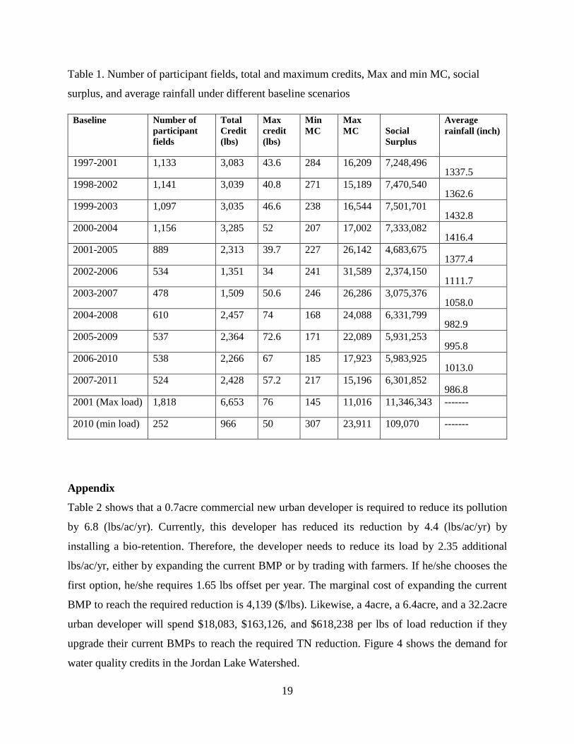
Table 1. Number of participant fields, total and maximum credits, Max and min MC, social
surplus, and average rainfall under different baseline scenarios
Baseline Number of participant fields
Total Credit (lbs)
Max credit (lbs)
Min MC
Max MC Social
Surplus
Average rainfall (inch)
1997-2001 1,133 3,083 43.6 284 16,209 7,248,496 1337.5
1998-2002 1,141 3,039 40.8 271 15,189 7,470,540 1362.6
1999-2003 1,097 3,035 46.6 238 16,544 7,501,701 1432.8
2000-2004 1,156 3,285 52 207 17,002 7,333,082 1416.4
2001-2005 889 2,313 39.7 227 26,142 4,683,675 1377.4
2002-2006 534 1,351 34 241 31,589 2,374,150 1111.7
2003-2007 478 1,509 50.6 246 26,286 3,075,376 1058.0
2004-2008 610 2,457 74 168 24,088 6,331,799 982.9
2005-2009 537 2,364 72.6 171 22,089 5,931,253 995.8
2006-2010 538 2,266 67 185 17,923 5,983,925 1013.0
2007-2011 524 2,428 57.2 217 15,196 6,301,852 986.8
2001 (Max load) 1,818 6,653 76 145 11,016 11,346,343 -------
2010 (min load) 252 966 50 307 23,911 109,070 -------
Appendix
Table 2 shows that a 0.7acre commercial new urban developer is required to reduce its pollution
by 6.8 (lbs/ac/yr). Currently, this developer has reduced its reduction by 4.4 (lbs/ac/yr) by
installing a bio-retention. Therefore, the developer needs to reduce its load by 2.35 additional
lbs/ac/yr, either by expanding the current BMP or by trading with farmers. If he/she chooses the
first option, he/she requires 1.65 lbs offset per year. The marginal cost of expanding the current
BMP to reach the required reduction is 4,139 ($/lbs). Likewise, a 4acre, a 6.4acre, and a 32.2acre
urban developer will spend $18,083, $163,126, and $618,238 per lbs of load reduction if they
upgrade their current BMPs to reach the required TN reduction. Figure 4 shows the demand for
water quality credits in the Jordan Lake Watershed.

20
Figure 4. Demand for water quality credits in Jordan Lake Watershed
0
5,000
10,000
15,000
20,000
25,000
0 1000 2000 3000 4000 5000 6000
P ($
)
Credit (lbs)

21
Table 2. New urban developers’ BMP size and BMP cost based on case study in Durham County, North Carolina
Development Type Size (ac)
Location BMP Current reduction (lbs/ac/yr)
Required reduction (lbs/ac/yr)
Total individual
offset (lbs/yr)
TC (NPV) for current
reduction ($)
TC (NPV) for required reduction ($) MC ($/lbs)
The Villas at Hope Valley Residential 4.00 Durham
BRC w/IWS1 2.1 2.4 1.36 123,051 129,199 18,083
City Center Commercial
Building 0.70 Durham BRC
w/IWS 4.4 6.8 1.65 35,612 45,338 4,139
Hendrick South Point
Commercial Auto Mall 32.20 Durham
2 Ponds and Sand
Filter 2.3 3.8 48.30 3,840,143 4,767,501 618,238
BCBS of NC Commercial 6.40 Durham
Wetland and Sand
Filter 2.2 4.9 17.28 921,651 1,362,092 163,126
1 Bio-retention cell with or without internal water storage