selecting a cost-e ective test case prioritization...
TRANSCRIPT

Selecting a Cost-Effective Test Case Prioritization Technique
Sebastian Elbaum,∗ Gregg Rothermel,† Satya Kanduri,‡ Alexey G. Malishevsky,§
January 8, 2003
Abstract
Regression testing is an expensive testing process used to validate modified software and detectwhether new faults have been introduced into previously tested code. To reduce the cost of regressiontesting, software testers may prioritize their test cases so that those which are more important, by somemeasure, are run earlier in the regression testing process. One goal of prioritization is to increase atest suite’s rate of fault detection. Previous empirical studies have shown that several prioritizationtechniques can significantly improve rate of fault detection, but these studies have also shown that theeffectiveness of these techniques varies considerably across various attributes of the program, test suites,and modifications being considered. This variation makes it difficult for a practitioner to choose anappropriate prioritization technique for a given testing scenario. To address this problem, we analyzethe fault detection rates that result from applying several different prioritization techniques to severalprograms and modified versions. The results of our analyses provide insights into what types of prioriti-zation techniques are and are not appropriate under specific testing scenarios, and the conditions underwhich they are or are not appropriate. Our analysis approach can also be used by other researchers orpractitioners to determine the prioritization techniques appropriate to other workloads.
1 Introduction
Regression testing is an expensive testing process used to validate modified software and detect whether new
faults have been introduced into previously tested code. Test case prioritization techniques help engineers
execute regression tests in an order that achieves testing objectives earlier in the testing process. One testing
objective involves rate of fault detection – a measure of how quickly a test order detects faults. An improved
rate of fault detection can provide earlier feedback on the system under test, enable earlier debugging, and
increase the likelihood that, if testing is prematurely halted, those test cases that offer the greatest fault
detection ability in the available testing time will have been executed.
Numerous prioritization techniques have been described in the research literature [5, 6, 8, 19, 23]. Studies
[6, 18, 19] have shown that at least some of these techniques can significantly increase the rate of fault
detection of test suites in comparison to the rates achieved by unordered or randomly ordered test suites.
More recently, researchers at Microsoft [21] have applied prioritization to test suites for several multi-million
line software systems, and found it highly efficient even on such large systems.∗Department of Computer Science and Engineering, University of Nebraska – Lincoln, [email protected]†Department of Computer Science, Oregon State University, [email protected]‡Department of Computer Science and Engineering, University of Nebraska – Lincoln, [email protected]§Department of Computer Science, Oregon State University, [email protected]
1

These early indications of potential are encouraging; however, studies have also shown that the rates of
fault detection produced by prioritization techniques can vary significantly with several factors related to
program attributes, change attributes, and test suite characteristics [3, 4]. In several instances, techniques
have not performed as expected. For example, one might expect that techniques that take into account the
location of code changes would outperform techniques that simply consider test coverage without taking
changes into account, and this expectation is implicit in the technique implemented at Microsoft [21]. In
our empirical studies [6], however, we have often observed results contrary to this expectation. It is possible
that engineers choosing to prioritize for both coverage and change attributes may actually achieve poorer
rates of fault detection than if they prioritized just for coverage, or did not prioritize at all.
More generally, to use prioritization cost-effectively, practitioners must be able to assess which prioritiza-
tion techniques are likely to be most effective in their particular testing scenarios, i.e., given their particular
programs, test cases, and modifications. Toward this end, we might seek an algorithm which, given various
metrics about programs, modifications, and test suites, calculates and recommends the technique most likely
to succeed. The factors affecting prioritization success are, however, complex, and interact in complex ways
[3]. We do not possess sufficient empirical data to allow creation of such a general prediction algorithm, and
the complexities of gathering such data are such that it may be years before it can be available. Moreover,
even if we possessed a general prediction algorithm capable of distinguishing between existing prioritization
techniques, such an algorithm might not extend to additional techniques that may be created.
In this paper, therefore, we pursue an alternative approach. Using data obtained from the application
of several prioritization techniques to several substantial programs, we compare the performance of several
prioritization techniques in terms of effectiveness, and show how the results of this comparison can be used,
together with cost-benefit threshold information, to select a technique that is most likely to be cost-effective.
We then show how an analysis strategy based on classification trees can be incorporated into this approach
and used to improve the likelihood of selecting the most cost-effective technique.
Our results provide insight into the tradeoffs between techniques, and the conditions underlying those
tradeoffs, relative to the programs, test suites, and modified programs that we examine. If these results
generalize to other workloads, they could guide the informed selection of techniques by practitioners. More
generally, however, the analysis strategy we use demonstrably improves the prioritization technique selection
process, and can be used by researchers or practitioners to evaluate techniques in a manner appropriate to
their own testing scenarios.
The rest of this article is organized as follows. Section 2 describes the test case prioritization problem in
greater detail, presents a measure for assessing rate of fault detection and techniques for prioritizing tests,
and summarizes related work. Section 3 presents the details of our study, our results, and our approaches
for selecting appropriate techniques. Section 4 presents further discussion of our results, and concludes.
2

2 Test Case Prioritization
Rothermel et al. [19] define the test case prioritization problem and describe several issues relevant to its
solution; this section reviews the portions of that material that are necessary to understand this article.
The test case prioritization problem is defined as follows:
The Test Case Prioritization Problem:
Given: T , a test suite; PT , the set of permutations of T ; and f , a function from PT to the real
numbers.
Problem: Find T ′ ∈ PT such that (∀T ′′) (T ′′ ∈ PT ) (T ′′ 6= T ′) [f(T ′) ≥ f(T ′′)].
Here, PT represents the set of all possible prioritizations (orderings) of T , and f is a function that, applied
to any such ordering, yields an award value for that ordering.
There are many possible goals for prioritization. In this article, we focus on increasing the likelihood of
revealing faults earlier in the testing process. This goal can be described, informally, as one of improving a
test suite’s rate of fault detection. To quantify this goal, [19] introduced a metric, APFD, which measures
the weighted average of the percentage of faults detected over the life of the suite. APFD values range from
0 to 100; higher numbers imply faster (better) fault detection rates.
Let T be a test suite containing n test cases, and let F be a set of m faults revealed by T . Let TFi be the
first test case in ordering T ′ of T which reveals fault i. The APFD for test suite T ′ is given by the equation:
APFD = 1 − TF1 + TF2 + ... + TFm
nm+
12n
(1)
For example, consider a program with a test suite of five test cases, A through E, such that the program
contains eight faults detected by those test cases, as shown by the table in Figure 1.A. Consider two orders
of these test cases, order T1: A–B–C–D–E, and order T2: C–E–B–A–D. Figures 1.B and 1.C show the
percentages of faults detected versus the fraction of the test suite used, for these two orders, respectively.
The area inside the inscribed rectangles (dashed boxes) represents the weighted percentage of faults detected
over the corresponding fraction of the test suite. The solid lines connecting the corners of the inscribed
rectangles interpolate the gain in the percentage of detected faults. The area under the curve thus represents
the weighted average of the percentage of faults detected over the life of the test suite. Test order T1 (Figure
1.B) produces an APFD of 50%, and test order T2 (Figure 1.C) is a much “faster detecting” test order than
T1, (and in fact, an optimal order) with an APFD of 84.0%.
3

0.6 0.8
10
20
30
40
50
60
70
80
90
Test Suite Fraction
100
0
0 0.2 0.4 1.0
Test Case Order: A−B−C−D−E
Per
cent
Det
ecte
d F
aults
Area = 50%
1 2 3 4 5 6 7 8 9 10x xx x x xx x x x x x x x x x x
ABCDE
test fault
0.2 0.4 0.6 0.8 1.0
0
0
10
20
30
40
50
60
70
80
90
100
Test Suite Fraction
Test Case Order: C−E−B−A−D
Per
cent
Det
ecte
d F
aults
Area = 84%
A. Test suite and faults exposed B. APFD for prioritized test suite T1 C. APFD for prioritized test suite
Figure 1: Example illustrating the APFD measure.
2.1 Prioritization Techniques
Numerous prioritization techniques have been described in the research literature [5, 6, 8, 19, 23]. To date,
most proposed techniques have been code-based, relying on information relating test cases to coverage of
code elements, and a first dimension along which techniques can be distinguished is in terms of the type
of code elements they consider. For example, test cases can be prioritized in terms of the number of code
statements, basic blocks, or functions they executed on a previous version of the software. One technique
for doing this, total function coverage prioritization, simply sorts the test cases in the order of the number of
functions they cover, and if multiple test cases cover the same number of functions, orders these randomly.
A second dimension along which techniques can be distinguished involves the use of “feedback”. When
prioritizing test cases, having selected a particular test case as “next best”, information about that test case
can be used to re-evaluate the worth of test cases not yet chosen, prior to picking the next best test case.
For example, additional function coverage prioritization iteratively selects a test case that yields the greatest
function coverage, then adjusts the coverage information for remaining test cases to indicate their coverage
of functions not yet covered, and then repeats this process until all functions coverable by at least one test
case have been covered. At this point, the process is repeated on remaining test cases.
A third dimension along which techniques can be distinguished involves the use of other, non-coverage
based, sources of information in prioritization. One such source of information pertains to modifications. For
example, the amount of change undergone by a code element can be factored into prioritization, by weighting
the elements covered using a fault index indicating an amount of change [16]. Such a fault index can range
from a complex metric incorporating various factors related to the possible indicence of regressionfaults [6],
to a simple binary metric indicating “changed” or “not changed”. Other types of information suggested
4

in the literature [5, 6] include test cost estimates, fault severity estimates, estimates of fault propagation
probability, and usage statistics obtained through operational profiles; these can be used to adjust the weights
given to specific classes of test cases or coverable elements.
2.2 Related Work
In recent years, several researchers have addressed the test case prioritization problem and presented tech-
niques for addressing it.
Wong et al. [23] suggest prioritizing test cases according to the criterion of “increasing cost per additional
coverage”. The authors restrict their attention to prioritization of the subset of test cases selected from a
test suite by a safe regression test selection technique, and the selected test cases are only those test cases
that reach modified code, but other test cases could be placed after these for later execution. Thus, this
technique can be described as using feedback, modification information, and test cost information.
Rothermel et al. [18, 19] and Elbaum et al. [5, 6], in work summarized above, provide the first formal
definition of the prioritization problem and present metrics for measuring the rate of fault detection of test
suites. They define prioritization techniques including all of those described in Section 3.1, and present the
results of several empirical studies of those techniques.
Jones et al. [8] describe a technique for prioritizing test cases for use with the modified condition/decision
coverage (MCDC) criteria, this technique uses feedback, but no modification information.
Srivastava and Thiagarajan [21] present a technique for prioritizing test cases based on basic block
coverage, using both feedback and change information. The technique also differs from previous techniques
in that it computes flow graphs and coverage from binaries, and attempts to predict possible affects on
control flow following from code modifications. The authors describe the application of this technique to
several large systems at Microsoft, and provide data showing that the approach can be applied efficiently
to those systems. The authors also provide data suggesting that their prioritized test case orders achieve
coverage quickly, and can detect faults early; however, their studies do not compare their prioritized test
suites to other test suites, so it is not possible to say whether the results represent an improvement in rate
of fault detection over those that would be obtained with other orderings.
Kim and Porter [10] present a technique, which they refer to as a “history-based prioritization” technique,
in which information from previous regression testing cycles is used to better inform the selection of a subset
of an existing test suite for use on a modified version of a system. This technique is not, however, a
“prioritization technique” in the sense defined in the literature (and summarized earlier in this section),
because it imposes no ordering on test cases – the characteristic essential to the definition of prioritization.
Rather, the approach selects a subset of a test suite, using history information to determine which test cases
should be selected, and is more accurately described as a “regression test selection technique” [17].
5

Avritzer and Weyuker [1] present techniques for generating test cases that apply to software that can
be modeled by Markov chains, provided that operational profile data is available. Although the authors do
not use the term “prioritization”, their techniques generate test cases in an order that can cover a larger
proportion of the software states most likely to be reached in the field earlier in testing, essentially, prioritizing
the test cases in an order that increases the likelihood that faults more likely to be encountered in the field
will be uncovered earlier in testing. Though not concerned with the prioritization of existing test cases for
use in testing modified software, the approach provides an example of the application of prioritization in the
case in which test suites are not available.
Among the papers described above, only a few [5, 6, 18, 19] report results of studies or experiments
explicitly assessing the ability of prioritization techniques to improve rate of fault detection, relative to each
other or to unprioritized test suites. As reported in Section 1, however, these studies show that technique
effectiveness varies widely with a number of factors involving program, change characteristics, and test
suite characteristics. None of the techniques investigated have proven uniformly superior to others in all
situations. To make effective use of prioritization, practitioners require strategies for selecting the appropriate
techniques. To date, no such strategies have been provided.
3 Empirical Study
To assess whether, and under which conditions, specific code-based prioritization techniques are preferable
to other techniques, and to examine approaches for making such assessments, we designed and performed
an empirical study. We applied several prioritization techniques to test suites for several versions of several
non-trivial programs, and measured the rates of fault detection of the resulting test suites. We then used
this data to compare relative technique performance and investigate the factors affecting it, and provide
strategies for selecting appropriate techniques. This section describes the techniques we selected, the subject
programs and test suites we studied, and our results and findings.
3.1 Prioritization Techniques
As target prioritization techniques, we choose four heuristics that have been previously described in the
literature [5, 19] and investigated in empirical studies [5, 6, 18, 19], that could easily be (or have already
been) implemented by practitioners, and that allow us to examine two of the key dimensions of differences
among techniques: the uses of feedback and information on modifications. (For simplicity and to facilitate
comparison, we restricted our attention to function-coverage-based techniques). The four techniques were:
Total function coverage prioritization (total). Total function coverage prioritization sorts the test cases
in the order of function coverage achieved. If multiple test cases cover the same number of functions,
they are ordered randomly.
6

Additional function coverage prioritization (addtl). Additional function coverage prioritization combines
feedback with coverage information: it iteratively selects a test case that yields the greatest function
coverage, then adjusts the coverage information on subsequent test cases to indicate their coverage of
functions not yet covered, and then repeats this process, until all functions covered by at least one test
case have been covered. If multiple test cases cover the same number of functions not yet covered, they
are ordered randomly. When all functions have been covered, this process is repeated on remaining
test cases, until all have been ordered.
Total binary-diff function coverage prioritization (total-diff). Total binary-diff function coverage priori-
tization uses modification information, but without feedback: it sorts test cases in the order of their
coverage of functions that differ textually (as measured by a modified version of the Unix “diff” func-
tion). If multiple test cases cover the same number of differing functions, they are ordered randomly.
When all test cases that cover differing functions have been ordered, remaining test cases are ordered
using total function coverage prioritization.
Additional binary-diff function coverage prioritization (addtl-diff). Additional binary-diff function coverage
prioritization uses both feedback and modification information: it iteratively selects a test case that
yields the greatest coverage of functions that differ, then adjusts the coverage information on subsequent
test cases to indicate their coverage of functions not yet covered, and then repeats this process, until all
functions that differ and that have been covered by at least one test case have been covered. If multiple
test cases cover the same number of differing functions not yet covered, they are ordered randomly.
This process is repeated on remaining test cases, until all test cases that execute functions that differ
have been used; then, additional function coverage prioritization is applied to remaining test cases.
As a control technique, we also considered random orderings of test cases (random), which let us
determine whether the heuristics we examined obtained results better than might be obtained by chance.
3.2 Subject Programs and Test Suites
To reduce the likelihood that our results would be dependent on a specific set of programs, we used eight
C programs with different characteristics as subjects. Table 1 lists these programs and some of their salient
characteristics, including number of versions, number of non-comment, non-blank lines of code in the initial
version, number and size of the test suites used, and average number of faults present in the versions.
The preparation of these subjects involved several activities including instrumentation of programs to
measure coverage, standardization and automation of build process, construction of oracles based on outputs
of previous program versions, and scripts ranging from test harnesses to measurement computation scripts.
We also performed fault seeding and test suite construction for most subjects, as follows.
7

Subject Description KLOC Number of Number of Number of Avg. FaultsVersions Test Suites Test Cases per Version
bash Unix shell 49 10 2 1168, 19 7.8emp-server server module of internet game 68 10 2 1985, 32 10.0flex lexical analyzer generator 8 5 1 567 4.5grep pattern search utility 11 5 1 809 2.8gzip data compression/decompression 5 6 1 217 11.8make build manager 18 5 1 1043 4.0sed stream editor 8 2 1 1293 4.5xearth view earth from space 24 3 1 539 3.5
Table 1: Subject Characteristics
Test Suites. To conduct our study we required test cases for our programs. For emp-server, flex, grep,
gzip, make, sed, and xearth no test cases were available. To construct test cases representative of those that
might be created in practice for these programs, we adapted a process defined initially by Hutchins et al. [7]
for their study of test adequacy criteria. We used the documentation on the programs, and the parameters
and special effects we determined to be associated with each program, as informal specifications. We used
these informal specifications, together with the category partition method and an implementation of the
TSL tool [2, 13] to construct a suite of test cases that exercise each parameter, special effect, and erroneous
condition affecting program behavior. We then augmented those test suites with additional test cases to
increase code coverage (measured at the statement level). We created these suites for the base versions of the
programs; they served as regression suites for subsequent versions. Bash was somewhat different in that it
had been released with test suites composed of test cases from previous versions and new test cases designed
to validate added functionality. However, some of these suites also contained test cases that were obsolete
for later versions of the system. Thus, we decided to use the test cases from release 2.0 of the system because
most these worked on all releases, and we updated this suite to test additional features (considering the
reference documentation for Bash [15] as an informal specification) and increase coverage of functions.
Faults. We wished to evaluate the performance of prioritization with respect to detection of regression
faults, that is, faults created in a program version as a result of the modifications that produced that version.
Such faults were not available with our subject programs; thus, to obtain them, we followed a procedure
similar to one defined and employed in several previous studies of testing techniques [7, 24, 25], as follows.
First, the two labs involved in the study recruited graduate and undergraduate students in computer science
with at least two years of C programming experience. Then, the students thus recruited were instructed to
insert faults that were as realistic as possible based on their experience, and that involved code deleted from,
inserted into, or modified between the versions. To further direct their efforts, the fault seeders were given
the following list of types of faults (adapted from the fault classification presented in [12]) to consider:
8

• Faults associated with variables, such as with definitions of variables, redefinitions of variables, deletions
of variables, or changes in values of variables in assignment statements.
• Faults associated with control flow, such as addition of new blocks of code, deletions of paths, redefi-
nitions of execution conditions, removal of blocks, changes in order of execution, new calls to external
functions, removal of calls to external functions, addition of functions, or deletions of functions.
• Faults associated with memory allocation, such as not freeing allocated memory, failing to initialize
memory, or creating erroneous pointers.
Given ten potential faults seeded in each version of each program, we activated these faults individually,
and executed the test suites for the programs to determine which faults could be revealed by which test cases.
We excluded any potential faults that were not detected by any test cases: such faults are meaningless to
our measures and have no bearing on results. We also excluded any faults that were detected by more than
25% of the test cases; our assumption was that such easily detected faults would be detected by engineers
during their unit testing of modifications. The average number of faults remaining across all versions are
reported in the rightmost column of Table 1.
3.3 Results and Findings
We applied each of our five prioritization techniques to each of our subject programs (for each applicable
test suite), for each pair of sequential versions in turn. For each such application we computed the APFD of
the resulting prioritized test suite with respect to the faults in the subsequent version. We also computed an
approximate optimal APFD achievable for the given test suite and set of faults.1 This process produced 56
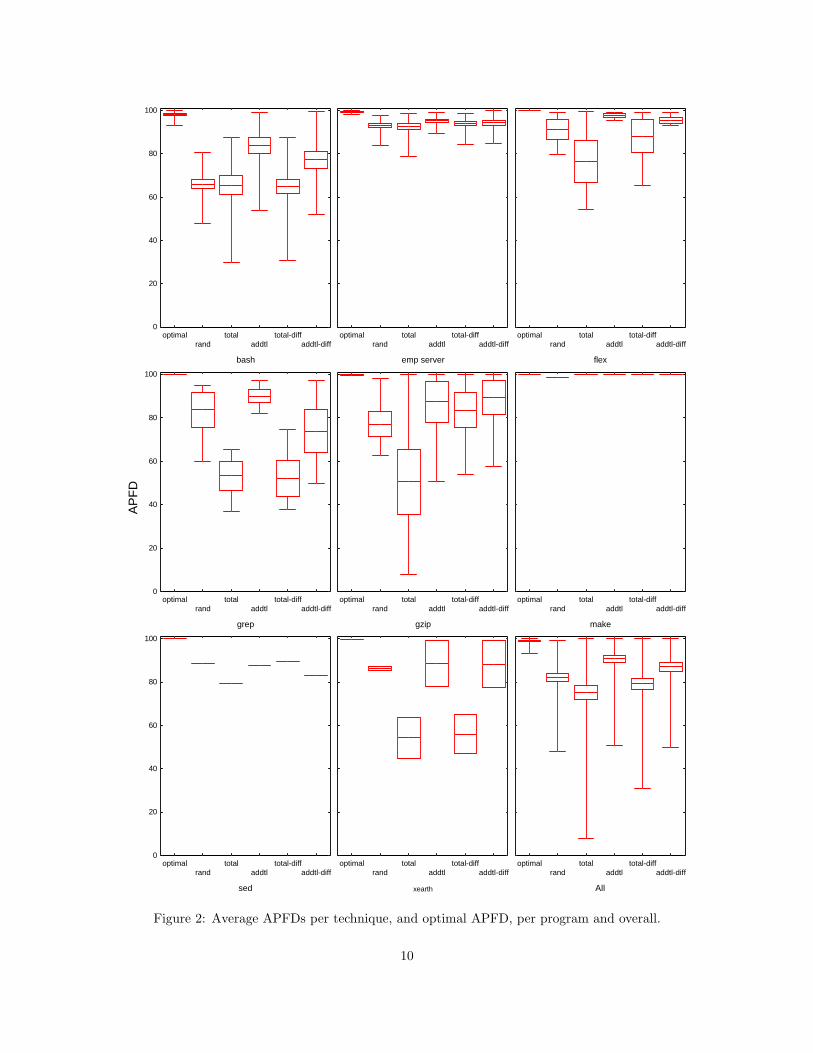
APFD values, which are represented in the box-plots shown in Figure 2.2 The figure contains separate plots
for each program and one plot summarizing“all programs” (bottom-right). Each plot contains a box showing
the distribution of APFD scores for each of the five techniques, and the optimal APFD scores possible.
Overall, the APFD results shown in Figure 2 are similar to those observed in previous studies [5, 6,
18, 19]. Techniques using feedback (addtl and addtl-diff) usually produced better prioritization results
than random, and in some cases (e.g., flex) approximated optimal ordering. In contrast, the simplest
prioritization technique, total, produced an average APFD lower than or equal to that produced by random.
Considering the data for all subjects, we note that techniques without feedback tended to have lower APFD
values and exhibit greater variance in APFD than techniques with feedback. We also found that the use1This approximate optimal APFD was calculated through a greedy heuristic that orders test cases in terms of the number
of as-yet-unexposed faults they uncover. Although not a practical prioritization technique per se (because it assumes priorknowledge of which tests expose which faults), this heuristic provides an approximate upper bound on prioritization results.
2Box plots provide a concise display of a distribution. The central line in each box marks the mean value. The edges of thebox are bounded by the standard error. The whiskers extend to the minimum and maximum data points observed.
9
AP
FD
bash
optimalrand
totaladdtl
total-diffaddtl-diff
0
20
40
60
80
100
emp server
optimalrand
totaladdtl
total-diffaddtl-diff
flex
optimalrand
totaladdtl
total-diffaddtl-diff
grep
optimalrand
totaladdtl
total-diffaddtl-diff
0
20
40
60
80
100
gzip
optimalrand
totaladdtl
total-diffaddtl-diff
make
optimalrand
totaladdtl
total-diffaddtl-diff
sed
optimalrand
totaladdtl
total-diffaddtl-diff
0
20
40
60
80
100
xearth
optimalrand
totaladdtl
total-diffaddtl-diff
All
optimalrand
totaladdtl
total-diffaddtl-diff
Figure 2: Average APFDs per technique, and optimal APFD, per program and overall.
10

of modification information (indicated by the -diff suffix) sometimes improved the total technique (e.g, on
flex, gzip, sed, and xearth), but often caused the addtl technique to behave more poorly.
Figure 2 also shows the degree to which APFD values varied across subjects and versions. For example,
on some subjects (e.g., gzip) there was large variance in APFD values for all techniques, while on others
(e.g., make) APFD values were relatively consistent for all techniques. On still other subjects (e.g., flex),
some techniques exhibited wide variance while others did not. The relative performances of techniques also
differed across subjects; for example, on grep, the mean APFD value for addtl was 20 points greater than
the mean APFD value for addtl-diff, while on gzip, the mean APFD value for addtl-diff was better than
the mean APFD value for addtl.
3.3.1 Prioritization Instances and Cost-Benefit Thresholds
A practitioner turning to Figure 2 for help in selecting a prioritization technique could easily be misled.
For example, although total-diff’s mean APFD was worse than random’s mean APFD on most programs,
on 56% of all individual applications total-diff was superior to random. In general, measures of central
tendency such as the mean are appropriate to characterize an aspect of a distribution, but they do not
provide a way to characterize how likely we are, in selecting a technique, to be correct in our selection.
A different strategy for assessing the tradeoffs between prioritization techniques, that does provide a way
to characterize the likelihood of selecting a technique correctly, can be obtained by comparing the numbers
of applications in which the performances of prioritization techniques differ. Toward this end, we define a
prioritization instance as a single application of a given prioritization technique to a given version and test
suite. To compare two prioritization techniques, as an initial strategy, we calculate the number of instances
in which the first technique generates a higher APFD than the second.
When making this comparison, however, we also consider an additional factor. A difference in APFD of
k% may or may not be practically important to a practitioner, depending on various cost factors associated
with the practitioner’s testing process [6]. To assume that a “higher” APFD implies a better technique,
independent of cost factors, is an oversimplification that may lead to inaccurate choices among techniques.
Cost models for prioritization [11] can be used to determine, for a given testing scenario, the amount
of difference in APFD that may yield desirable practical benefits, by associating APFD differences with
measurable attributes such as dollar costs. Without constraining our analysis to specific costs, however, we
can analyze cost-benefits more generally by using an abstract notion of the amount of difference in APFD
that we refer to as a cost-benefit threshold: a percentage difference in APFD that must be exceeded in order
for that APFD gain to be beneficial.
Table 2 compares the performances of the techniques we investigated in our study in terms of prioritization
instances, conditioned on several different cost-benefit thresholds. The table displays, for each pairwise
11

Row Techniques Cost-Benefit Threshold# Compared 0% 1% 5% 10% 25%1 total vs. random 41 39 21 5 22 addtl. vs. random 79 70 37 32 203 addtl vs. total 61 61 52 39 304 total-diff vs. random 57 41 16 9 25 total-diff vs. total 55 50 34 16 56 total-diff vs. addtl 23 16 7 4 27 addtl-diff vs. random 68 59 30 25 148 addtl-diff vs. total 63 63 46 37 149 addtl-diff vs. addtl 41 25 7 2 2
10 addtl-diff vs. total-diff 50 41 30 25 14
Table 2: Percentage of prioritization instances in which the first technique compared is better than thesecond technique compared under a given cost-benefit threshold.
technique comparison (one per row), the percentage of prioritization instances in which each technique
was worth applying, across five cost-benefit threshold values (0%, 1%, 5%, 10%, and 25%). Within each
comparison, for each cost-benefit threshold k, we list the percentages of prioritization instances in which the
first technique of the two compared (the leftmost technique listed in column 2) produced an APFD value
exceeding that of the second technique by k% or more, and thus, should be the preferred technique under
threshold k. Put differently, the numbers contained in the table’s cells under a given threshold k indicate
the probability that the first technique would achieve an APFD k% better than the second technique, across
the instances in which the techniques were applied.
The data in the table serves as the basis for a prioritization technique selection strategy (henceforth
referred to as the basic instance-and-threshold strategy). For example, considering row 2, a practitioner
can claim some confidence that benefits will be obtained, at low cost-benefit thresholds, by employing
addtl rather than random, because such benefits were observed in 79% of the instances considered for
threshold 0%, and 70% of the instances considered for threshold 1%. On the other hand, considering row 9,
a practitioner expecting to obtain benefits by incorporating modification information into addtl stands more
chances of being incorrect than correct, for all cost-benefit thresholds, and a practitioner choosing between
total and random would select appropriately on more occasions by just choosing random.
The table also shows that, when the practitioner becomes more demanding with respect to cost-benefit
threshold, the recommended technique shifts. For example (row 2), although addtl is preferable to random
when thresholds are low (0% or 1%), as cost-benefit threshold reaches 5% there is a larger probability that
the use of feedback is not worthwhile. Also, at cost benefit thresholds of 5% or higher, comparing random
to any heuristic (rows 1, 2, 4, and 7), there are always more instances in which random is preferable.
It is also interesting to observe how the rates at which percentages change vary across comparisons. For
example, the probability that addtl is preferable to total decreases more slowly, as threshold increases,
12

than does the probability that addtl is preferable to random; this indicates a smoother transition between
threshold levels.
Finally, although we cannot claim that the particular results presented in the table generalize to other
programs, versions, and test suites, with further experimentation we hope to improve the generality of the
information presented. Meanwhile, a practitioner could collect similar data on their own systems and employ
the method just described to determine which techniques to employ on those systems in future regression
testing efforts.
3.3.2 Improving Technique Selection using Testing Scenario Characteristics
The basic instance-and-threshold strategy for comparing and selecting prioritization techniques is based
exclusively on comparisons of the APFD values achieved by two techniques, relative to a given cost-benefit
threshold; it is simple and, our data shows, can be effective in some cases. In other cases, however, this
strategy may not be helpful. For example, the table reveals that the chance of achieving higher APFDs by
adding feedback to the total-diff technique (i.e, by using addtl-diff) is 50/50. That is, the practitioner can
obtain the same level of certainty that they are choosing the best technique through a coin-toss.
Whether or not this strategy is effective, it seems possible that a second strategy considering the charac-
teristics of the testing scenario (the particular program, modifications, and test suite involved), could increase
the probability of choosing a technique correctly. We call this second strategy the enhanced instance-and-
threshold strategy, and to investigate it we followed a two step process. First, we characterized the collected
prioritization instances by computing a set of metrics related to testing scenarios. Second, we used these
metrics to refine the guidelines for selecting techniques by building classification trees.
Classification Trees and their Application
Classification trees have been used frequently in previous software engineering research. For example, classifi-
cation trees have been used to classify modules as fault prone or not fault prone [9] and to predict components
for which development effort is likely to be high [14, 20]. In our context, we use classification trees to predict
whether a certain testing scenario facilitates the use of a prioritization technique by measuring program,
test suite, and change characteristics that hold for that particular scenario. Classification trees can help
with this for several reasons. First, unlike more traditional statistical techniques,3 classification trees are not
constrained by the underlying population distribution. Second, their hierarchical nature makes them easy
to interpret, which could facilitate their adoption by practitioners. Third, the trees can be decomposed into
a set of rules that make the decision process straightforward.3For example, consider the differences between classification trees and discriminant analysis. Instead of producing a set
of coefficients defining the single linear combination of the independent variables that best differentiates the groups in theindependent variable where all predictor variables are considered simultaneously, decision trees employ a hierarchical form,where decisions are made sequentially on each independent variable.
13

The generation of a classification tree starts from a set of observations that constitute a training or learning
set for which a property that must be forecasted is known. For example, for the question of whether feedback
is effective, the learning set must include, for each prioritization instance, whether feedback was beneficial
or not. In addition, each prioritization instance has a set of associated values corresponding to a number
of independent variables. The tree generation process begins by splitting the learning set (starting node)
into two subgroups (child nodes). The method we used for splitting, CART (Classification and Regression
Trees), uses an “exhaustive search for univariate splits” method for categorical predictor variables [22], in
which all possible splits for each predictor variable at each node are examined to find the split producing
the largest improvement in goodness of fit. We employed the Gini goodness of fit measure, which reaches
a value of zero when only one class is present at a node and reaches its maximum value when class sizes at
the node are equal. The process is repeated recursively for each node until a stopping rule is reached.
Tree evaluation is commonly performed through misclassification rates. A portion of the cases are des-
ignated as belonging to the learning sample and the remaining cases are designated as belonging to the test
sample. The predictive model defined by the tree can then be developed using the cases in the learning
sample, and its predictive accuracy can be assessed using the cases in the test sample.
In our application of the approach, we used 25% of our observations as the test sample, which left 42
observations in the learning set. Also, to check the stability of the trees, we used v-random cross validation
within the learning sample. This cross validation involved selecting five random subsamples of equal size from
the learning sample and computing the classification tree of the specified size five times, each time omitting
one of the subsamples from the computation and using that subsample as a test sample for cross-validation.
Thus, each subsample was used four times in the learning sample and just once as the test sample.
In addition, we made the following assumptions while generating trees. First, since the prioritization
techniques we examined are relatively simple, we assumed that their cost is equivalent. We also assumed
the same misclassification cost, independent of the predicted outcome. Second, we assumed that the prior
probability of a technique being successful is proportional to the percentage of observations in the learning
set where that technique generated an APFD value greater than its counterpart (e.g., addtl is assumed to
be successful in 70% of the scenarios for a 1% cost-benefit). Third, splitting on the predictor variables of the
learning set continued until each terminal node in the classification tree had no more than 25% of misplaced
scenarios (Fact/frac option in Statistica).
The independent variables we considered were obtained from previous studies [3, 4] which identified and
classified the sources of variation observed in the prioritization techniques’s effectiveness. Those sources
involve program, test suite and change characteristics. The resulting metric set (Table 3) is the result of a
refinement process in which several of the originally proposed metrics were discarded based on their marginal
contribution to the observed variation in APFD.
14

Metric Description Mean Median Std. Dev.A FSIZE mean function size 54 46 19AN CHOC mean number of changes lines per changed function 9 7 6P FCH C percentage of functions changed and covered 12 7 15P CH L percentage of changed LOC 11 3 17P TRCHF percentage of tests reaching a changed function 94 100 23AP FET mean percentage of functions executed by a test 33 36 9A TESTS CHF mean number of tests going through changed functions 40 45 20P CH INDEX probability of executing changed functions 16 9 18
Table 3: Metrics collected over the 56 applications of prioritization techniques to our subject programs.
Results
We generated classification trees for each pair of techniques compared (each row) in Table 2, beginning with
the pairs for which the application was successful in producing refinements (rows 1, 2, 3, 5, 8, and 10),
followed by the other pairs. (We generated trees only for the cost-benefit threshold of 1%. This choice was
arbitrary and does not imply any loss of generality for the approach.)
1. total versus random
We begin by comparing total and random. Figure 3 presents the tree that results from applying the
classification tree approach considering these two techniques. The tree starts with the top decision node
(node “1”). Each node contains a histogram representing the frequency distribution of the techniques being
compared (heights of the columns are proportional to the frequencies); the legend at upper left identifies the
techniques to which the bars in the histograms correspond. Each node also contains a label indicating the
dominant technique in that node. The root node, node 1, is split forming two new nodes; the text beneath
the root node describes the rule determining the split. In Figure 3 this rule indicates that instances with
AP FET ≤ 35% are sent to node 2 and classified as cases in which random should be used, and instances
with AP FET values greater than 35% are assigned to node 3 and classified as cases in which total should
be used. The values of 18 and 24 printed above nodes 2 and 3, respectively, indicate the number of cases
sent to each of these two child nodes.
The tree indicates that total worked best on testing scenarios in which test cases executed relatively larger
percentages of the functions in the system tested, leading to a higher probability of covering a changed
function. On the other hand, total did not perform as well in scenarios in which test cases had smaller
“footprints”, where the probability of not executing a faulty function is accentuated.
We next employed the test set to assess tree accuracy. The results are presented in Table 4. The rows in
this table correspond to the technique predictions for the instances, and the columns indicate actual observed
results. For example, in four test instances total was the best performer and this was correctly predicted,
whereas in two instances our predictions were incorrect because random did better. Overall, we observe
15

1
2 3
AP_FET <= 35
18 24
random
random total
totalrandom
Figure 3: Classification tree for total versus random.
Techniques total randomtotal 4 2random 0 8Misclassification Rates 0/4 = 0% 2/10 = 20%
Table 4: Classification accuracy on test sample - total versus random
that with just one metric, the tree could discern with 100% accuracy the instances in which total would be
preferable to random, and with 80% accuracy the instances in which total would not outperform random.
Recall that a practitioner following the guidelines given in Table 2, at cost-benefit threshold 1%, would
discard total and employ no prioritization technique, missing an opportunity for improvement in 39% of
the instances. Following the guidelines presented in the classification tree would increase the likelihood
of selecting the appropriate prioritization technique. Utilizing the misclassification rates (MR) and prior
probabilities (PP) from Table 2, a practitioner employing the tree would select the appropriate technique in
88% of the instances:
(1 − MRtotal) ∗ PPtotal + (1 − MRrandom) ∗ PPrandom = (1 − 0) ∗ 39% + (1 − .20) ∗ 61%) = 88% (2)
2. addtl versus random
Figure 4 presents the classification tree that results from comparing addtl and random. This tree
contains two splits. The first split is based on A FSIZE, indicating that programs with average function size
over 90 LOC are less likely to provide instances in which addtl is preferable to random. The second split
16

1
2 3
4 5
A_FSIZE <= 90
AN_CHOC <= 20
39 3
37 2
addtl
addtl random
addtl random
addtlrandom
Figure 4: Classification tree for addtl versus random.
Techniques addtl randomaddtl 10 3random 0 1Misclassification Rates 0/10 = 0% 3/4 = 75%
Table 5: Classification accuracy on test sample - addtl versus random
employs the AN CHOC metric with a value of 20, suggesting that functions in which average change size
is greater than 20 reduce the potential of addtl in comparison to random. Overall, programs with large
functions or functions with many changes tend to constrain the power of addtl. This could be caused by
the greedy nature of addtl and the fact that we employed it at the function coverage level. As such, even if
a function has a lot of change or is large, addtl seeks to cover it once, which may delay exposure of faults.
Table 5 assesses the accuracy of this tree. The misclassification rates indicate that, using the tree, we may
over-predict the cases in which addtl will be preferable. Still, the guidelines from Table 2 (at cost-benefit
level 1%) would lead a practitioner to choose addtl in all cases, missing an opportunity to do better in 30%
of the instances in which random is at least as good as addtl. The refined strategy increases the likelihood
of selecting the appropriate prioritization strategy to 78% of the cases (78% = (1-0) * 70% + (1-.75) * 30%).
3. addtl versus total
Figure 5 presents the classification tree that results from comparing addtl to total. This tree also
contains two splits. AP FET is again the first discriminator and, as in the preceding tree, smaller AP FET
17

1
2 3
4 5
AP_FET <= 35
P_CH_L < =26
18 24
20 4
addtl
addtl total
total addtl
totaladdtl
Figure 5: Classification tree for addtl versus total.
Techniques addtl totaladdtl 8 1total 1 3Misclassification Rates 1/9 = 11% 1/4 = 25%
Table 6: Classification accuracy on test sample - addtl versus total.
values do not benefit total. We believe that the availability of test cases focusing on specific functionality
(instead of exercising most of the system) are one determinant for whether feedback techniques prosper.
Node 3 is split again into two nodes based on the P CH L metric. The tree indicates that more changes are
likely to help feedback (assuming those changes are distributed).
Table 6 indicates that in this case, misclassification occurs primarily due to over-prediction on behalf of
addtl on instances in which it does not provide gains. Still, a practitioner has much to gain by using just
two metrics and the classification tree. Without using this information, addtl would be selected because
it performs better than total 61% of the time However, a practitioner employing the tree would select the
appropriate technique in 85% of the instances (85% = (1-.11) * 61% + (1-.20)* 39%).
5. total-diff vs total
Figure 6 presents the classification tree that results from comparing total-diff and total. This tree
contains three splits. The first split is based on AP FET, again indicating that higher percentages of
functions executed per test do promote the effectiveness of total. Node three is split based on P CH L,
18

1
2 3
4 5
6 7
AP_FET <= 35
P_CH_L <= 1
A_TESTS_CCHF <= 46
18 24
9 15
5 10
total
total-diff total
total total-diff
total-diff total
totaltotal-diff
Figure 6: Classification tree for total versus total-diff.
Techniques total total-difftotal 5 0total-diff 2 7Misclassification Rates 2/7 = 29% 0/7 = 0%
Table 7: Classification accuracy on test sample - total versus total-diff.
indicating that total is more likely to be beneficial if the percentage of changed lines of code is less than 1%.
The last split occurs on node five based on A TESTS CCHF. If the percentage of tests covering changed
functions is less than or equal to 46%, then incorporation of diff information seems to be helpful. Intuitively,
if the tests have a greater overlap covering changed functions, then total can potentially do as well as
total-diff since the use of modification information does not add much value.
Table 7 indicates that the tree mispredicted 29% of the instances in which total-diff was not beneficial,
but was very accurate in identifying instances in total-diff outperforms total. A practitioner employing
this tree would need to compute three metrics. Such effort would be compensated for, however, with an
86% probability of selecting the appropriate technique (86% = (1-.29) * 50% + (1-0) * 50%). Note that the
probability of selecting the appropriate technique without using the tree was 50%.
19

1
2 3
4 5
6 7
AP_FET <= 35
P_CH_L <= 1
A_TESTS_CCHF <= 48
18 24
9 15
6 9
addtl-diff
addtl-diff total
total addtl-diff
addtl-diff total
totaladdtl-diff
Figure 7: Classification tree for addtl-diff versus total.
Techniques addtl-diff totaladdtl-diff 3 0total 1 10Misclassification Rates 1/4 = 25% 0/10 = 0%
Table 8: Classification accuracy on test sample - addtl-diff versus total
8. addtl-diff vs total
A practitioner trying to determine whether to incorporate both change information and feedback into
total would employ the tree in Figure 7. The resulting tree has the same nodes and splitting metrics as the
one introduced in Figure 6. The misclassification rates from Table 8 indicate that a practitioner following
this tree would have an 84% probability of selecting the appropriate technique for a given scenario (84% =
(1-.25) * 63% + (1-0) * 37%), as opposed to 63% without using the tree.
10. addtl-diff vs total-diff
The tree in Figure 8 concerns the situation in which a practitioner using modification information must
decide whether or not to incorporate feedback. The figure indicates that with just one split based on the
P CH INDEX metric the leaf nodes are reached. Table 9 shows that this tree predicts addtl-diff to be
20

1
2 3
P_CH_INDEX <= 2.5
12 30
total-diff
total-diff addtl-diff
total-diffaddtl-diff
Figure 8: Classification tree for addtl-diff versus total-diff.
Techniques addtl-diff total-diffaddtl-diff 6 5total-diff 0 3Misclassification Rates 0/6 = 0% 5/8 = 63%
Table 9: Classification accuracy on test sample - addtl-diff versus total-diff
preferable to total-diff innacurrately in several instances. Yet, a practitioner following this tree would have
a 78% probability of choosing the appropriate technique (78% = (1-0) * 41% + (1-.63) * 59), which is greater
than the 63% chance of choosing correctly without the tree.
Remaining cases.
For four pairs of technique comparisons, classification trees did not provide additional selection power:
total-diff versus random, total-diff versus addtl, addtl-diff versus random, and addtl-diff versus
addtl. In these cases, no tree produced gains surpassing those that a practitioner could obtain by following
Table 2, and thus, trees were of no value. One possible reason for lack of effectiveness in classification trees
in these four cases could be that the attributes we captured are not able to fully explain the differences
in technique performance. Another possible reason is the limited number of observations available; more
observations could improve our understanding and enable the creation of useful classification trees.
It is interesting to note, however, that all comparisons in which a tree could not be constructed involved
a comparison with a technique using modification information. Modification information seems, in some
cases, to add variability in a manner that we cannot predict. Such variability could be caused, for example,
21

by the accuracy of the tools that determine modifications, or in the way in which modification information is
combined with coverage information. Still, it seems that the usage of modification information is not always
recommendable, and its success may be difficult to predict.
4 Discussion and Conclusions
We have presented a study of five prioritization techniques across eight systems. Although previous studies
of test case prioritization [5, 6, 18, 19] have been conducted, the set of subjects we have considered form the
largest set of non-trivial programs employed to date to quantify the relative effectiveness of prioritization
techniques at improving the rate of fault detection of test suites.4 Our results regarding the effectiveness
of the techniques confirm previous findings [5, 6, 18, 19], among them the fact that the performance of
test case prioritization techniques varies significantly with program attributes, change attributes, test suite
characteristics, and their interaction.
These results support the search for strategies by which practitioners could choose appropriate priori-
tization techniques for their particular testing scenarios, and we have proposed two such strategies. The
basic instance-and-threshold strategy, introduced in Section 3.3.1, recommends the technique that has been
successful in the largest proportion of instances in the past, accounting for cost-benefit thresholds. The
enhanced instance-and-threshold strategy, introduced in Section 3.3.2, adds into consideration the attributes
of a particular testing scenario, using metrics to characterize scenarios, and employing classification trees to
improve the likelihood of recommending the proper technique for each particular case.
The relative effectiveness of these two strategies for a cost-benefit threshold of 1% is summarized in Table
10. Each row introduces the techniques being compared, the probability for recommending the appropriate
technique for a given scenario under each strategy, and the gain generated by the enhanced strategy with
respect to the basic strategy. For example, in the first row, we see that a practitioner employing the basic
instance-and-threshold strategy would have a 61% likelihood of selecting the most effective technique. A
practitioner using the enhanced strategy, however, would have an 88% likelihood of selecting the most
effective strategy (at the cost of computing AP FET and following the classification tree introduced in the
previous section). The effectiveness of these strategies on the workloads we considered demonstrates their
viability for evaluating techniques in other scenarios introduced by researchers or practitioners.
In this work we have assumed that the prioritization techniques examined have equivalent costs. For
the relatively simple techniques we have considered, all operating at the level of function coverage and
using binary “diff” decisions that could be retrieved from configuration management, this assumption seems
reasonable. To extend these comparisons to other classes of techniques, however, this assumption is less4The preparation of such subjects is tedious and time consuming, and most likely this is the primary reason this type of
study has infrequently been attempted relative to software regression testing. For example, the fault seeding process requiresapproximately 80 person-hours per successful fault (that is exposed by some test cases).
22

Likelihood of StrategyRow # Techniques Compared Correct Recommendation Refinement
Basic Enhanced GainStrategy Strategy
1 total vs. random 61% 88% 17%2 addtl. vs. random 70% 78% 8%3 addtl vs. total 61% 85% 24%4 total-diff vs. random 59% 86% 27%5 total-diff vs. total 50% – –6 total-diff vs. addtl 84% – –7 addtl-diff vs. random 59% – –8 addtl-diff vs. total 63% 84% 21%9 addtl-diff vs. addtl 75% – –
10 addtl-diff vs. total-diff 59% 78% 19%
Table 10: Strategies for prioritization technique selection.
reasonable. Techniques that incorporate test cost or module criticality information, or those that operate at
finer grained levels of coverage, present different cost-benefits tradeoffs. These tradeoffs can be modelled as
described in [11], and related to cost-benefit thresholds, allowing comparisons of differing-cost techniques,
but this approach needs to be investigated empirically.
The most pressing need for future work, however, involves additional studies of prioritization applied to
a wider variety of programs, modified programs, test suites, and faults. Such studies could help us extend
the generality of our conclusions about relative technique efficacy. Further data will also help us better
understand the characteristics influencing cost-effectiveness, and help us further differentiate techniques
through additional metrics and the classification tree approach. The need for such studies is particularly
acute because software professionals are beginning to employ test case prioritization in practice [21], and
our results show that some of the expectations we might have about technique effectiveness (e.g. “adding
modification information will improve rate of fault detection”) can be incorrect. Practitioners relying on
such expectations may actually, and unwittingly, be harming their test suites’ rates of fault detection. Only
through careful empirical work can we transform such problematic expectations into useful engineering
strategies.
Acknowledgments
This work was supported in part by the NSF Information Technology Research program under Awards
CCR-0080898 and CCR-0080900 to University of Nebraska, Lincoln and Oregon State University. We are
especially grateful to the members of the MAPSTEXT and Galileo research groups for their assistance in
preparing subject programs.
23

References
[1] A. Avritzer and E. J. Weyuker. The automatic generation of load test suites and the assessment of the
resulting software. IEEE Transactions on Software Engineering, 21(9):705–716, Sept. 1995.
[2] M. Balcer, W. Hasling, and T. Ostrand. Automatic generation of test scripts from formal test speci-
fications. In Proceedings of the 3rd Symposium on Software Testing, Analysis, and Verification, pages
210–218, Dec. 1989.
[3] S. Elbaum, D. Gable, and G. Rothermel. Understanding and measuring the sources of variation in the
prioritization of regression test suites. In Proceedings of the Seventh International Software Metrics
Symposium. Institute of Electrical and Electronics Engineers, Inc., April 2001.
[4] S. Elbaum, P. Kallakuri, A. Malishevsky, G. Rothermel, and S. Kanduri. Understanding the effects of
changes on the cost-effectiveness of regression testing techniques. Technical Report 020701, University
of Nebraska - Lincoln, July 2002.
[5] S. Elbaum, A. Malishevsky, and G. Rothermel. Incorporating varying test costs and fault severities
into test case prioritization. In International Conference on Software Engineering, pages 329–338, May
2001.
[6] S. Elbaum, A. Malishevsky, and G. Rothermel. Test case prioritization: A family of empirical studies.
IEEE Transactions of Software Engineering, 28(2):159–182, February 2002.
[7] M. Hutchins, H. Foster, T. Goradia, and T. Ostrand. Experiments on the effectiveness of dataflow- and
controlflow-based te st adequacy criteria. In Proceedings of the International Conference on Software
Engineering, pages 191–200, May 1994.
[8] J. A. Jones and M. J. Harrold. Test-suite reduction and prioritization for modified condition/decision
coverage. In Proceedings of the International Conference on Software Maintenance, Nov. 2001.
[9] T. Khoshgoftaar, E. Allen, and J. Deng. Using regression trees to classify fault-prone software modules.
IEEE Transactions on Reliability, 51(4):455–462, 2002.
[10] J.-M. Kim and A. Porter. A history-based test prioritization technique for regression testing in resource
constrained environments. In Proceedings of the International Conference on Software Engineering, May
2002.
[11] A. Malishevsky, G. Rothermel, and S. Elbaum. Modeling the cost-benefits tradeoffs for regression testing
techniques. In Proceedings of the International Conference on Software Maintenance, Oct. 2002.
24

[12] A. P. Nikora and J. C. Munson. Software evolution and the fault process. In Proceedings of the Twenty
Third Annual Software Engineering Workshop, NASA/Goddard Space Flight Center, 1998.
[13] T. Ostrand and M. J. Balcer. The category-partition method for specifying and generating functional
tests. Communications of the ACM, 31(6), June 1988.
[14] A. Porter and R. Selby. Evaluating techniques for generating metric-based classification trees. The
Journal of Systems and Software, 12(3):209–218, 1990.
[15] C. Ramey and B. Fox. Bash Reference Manual. O’Reilly & Associates, Inc., Sebastopol, CA, 2.2 edition,
1998.
[16] G. Rothermel, S. Elbaum, A. Malishevsky, P. Kallakuri, and B. Davia. The impact of test suite
granularity on the cost-effectiveness of regression testing. In Proceedings of the 24th International
Conference on Software Engineering, pages 230–240, May 2002.
[17] G. Rothermel and M. Harrold. Analyzing regression test selection techniques. IEEE Transactions on
Software Engineering, 22(8):529–551, Aug. 1996.
[18] G. Rothermel, R. Untch, C. Chu, and M. J. Harrold. Test case prioritization: An empirical study. In
Proceedings of the International Conference on Software Maintenance, pages 179–188, 1999.
[19] G. Rothermel, R. H. Untch, C. Chu, and M. J. Harrold. Test case prioritization. IEEE Transactions
on Software Engineering, 27(10):929–948, October 2001.
[20] R. Selby and A. Porter. Learning from examples: Generation and evaluation of decision trees for
software resource analysis. IEEE Transactions on Software Engineering, 14(12):1743–1757, 1988.
[21] A. Srivastava and J. Thiagarajan. Effectively prioritizing tests in development environment. In Pro-
ceedings of the International Symposium on Software Testing and Analysis, pages 97–106, July 2002.
[22] Statsoft. Statistica. http://www.statsoft.com/exploratory.html.
[23] W. E. Wong, J. R. Horgan, H. London, and H. Agrawal. A study of effective regression in practice. In
Proceedings of the Eighth International Symposium on Software Reliability Engineering, pages 230–238,
November 1997.
[24] W. E. Wong, J. R. Horgan, S. London, and A. P. Mathur. Effect of test set size and block coverage
on the fault detection effectiveness. In Proceedings of the Fifth International Symposium on Software
Reliability Engineering, pages 230–238, Nov. 1994.
25

[25] W. E. Wong, J. R. Horgan, S. London, and A. P. Mathur. Effect of test set minimization on fault
detection effectiveness. In Proceedings of the 17th International Conference on Software Engineering,
pages 41–50, Apr. 1995.
26