selecting informative moments via lasso - people · estimator and di erent versions of...

SELECTING INFORMATIVE MOMENTS VIA LASSO

YE LUO

A. The traditional optimal GMM estimator is biased when there are many moments. This pa-

per considers the case when information is sparse, i.e., only a small set of the moment conditions is

strongly informative. We propose a LASSO based selection procedure in order to choose the informative

moments and then, using the selected moments, conduct optimal GMM. Our method can significantly re-

duce second-order bias of the optimal GMM estimator while retaining most of the information in the full

set of moments. The LASSO selection procedure allows the number of moments to be much larger than

the sample size. We establish bounds and asymptotics of the LASSO and post-LASSO estimators. Under

our approximate sparsity condition, both estimators are asymptotically normal and nearly efficient when

the number of strongly informative moments grows at a slow rate compared to the sample size. The for-

mulation of LASSO is a convex optimization problem and thus the computational cost is low compared to

other moment selection procedures such as those described in Donald, Imbens and Newey (2008). In an

IV setting with homoskedastic errors, our procedure reduces to the IV-LASSO method stated in Belloni,

Chen, Chernozhukov and Hansen (2012). We propose penalty terms using data-driven methods. Since

the construction of the penalties requires the knowledge of unknown parameters, we propose adaptive al-

gorithms which perform well globally. These algorithms can be applied to more general L1-penalization

problems when the penalties depend on the parameter to be estimated. In simulation experiments, the

LASSO-based GMM estimator performs well when compared to the optimal GMM estimator and CUE.

Keywords: GMM, Moment Selection, Many Moments, LASSO, Convex Optimization, Adap-tive Method.

1. I

The optimal two-step GMM estimator has been widely used in economic applications. It is quite

common to have an application with a large number of moment restrictions that can be used for esti-

mation and inference. For example, a conditional moment restriction provides an infinite number of

potential unconditional moments by allowing the use of different functions of the conditioning variable

Date: The present version is of Nov. 2, 2014. I am deeply grateful to my advisors Victor Chernozhukov, Jerry Hausman,

Anna Mikusheva and Whitney Newey for their guidance and suggestions to improve this paper. I thank Victor Chernozhukov

and Jerry Hausman for their long term encouragement during my PhD. I also thank Isaiah Andrews, Alexandre Belloni, Denis

Chetverikov, Kirill Evdokomov, Alfred Galichon, Yaroslav Muhkin, Martin Spindler and participants at MIT Econometrics

seminar for many helpful discussions. I thank Emily Gallagher for editing assistance. Contact: Department of Economics,

MIT. E-mail: [email protected]. All remaining errors are mine.1

2 YE LUO

as instruments. However, applying an efficient GMM estimator to many moment conditions typically

results in biased estimators and poor accuracy of confidence sets. Hansen, Hausman, Newey (2006)

shows that the presence of many valid instrumental variables (IV later) may improve efficiency, but the

inference procedure becomes inaccurate due to second order bias. If the number of moments exceeds

the sample size, then an efficient GMM estimator does not exist at all. The problem with many moments

arises from the efficient GMM’s need for the optimal weighting matrix, which is an inverse of a large

dimensional random matrix. The ill-posedeness of the inversion problem leads to poor performance

of the optimal GMM estimator. However, simply throwing out over-identified moments is undesirable

due to efficiency losses.

The main goal of this paper is to improve the GMM procedure by selecting informative moment

conditions from a large set of available moments. The selection procedure proposed in this paper

utilizes the basic spirit of regression-LASSO, using the L1 penalty to find a nearly optimal combination

of moment conditions. The goal is to select moments without loss of asymptotic efficiency but that will

guarantee the accurate coverage property of post selection inferences.

The main assumption needed to ensure the validity of the suggested procedure is approximate spar-

sity. The exact sparsity assumption means that all but a relatively small (though increasing with the

sample size) number of moments is absolutely uninformative about the parameter we are trying to esti-

mate. Approximate sparsity weakens this condition by allowing all moments to have some information

about the parameter of interest but, in fact, the majority of moments has so little informational content

that no loss of asymptotic efficiency occurs from not using those moments. The number and identity

of truly informative moments are unknown, but we need to impose bounds on the growth rate of the

number of informative moments requiring that it be much smaller than the sample size.

The LASSO method proposed in this paper could be viewed as a complementary method to the

traditional methods for the many moments problem. We provide a description of the convergence rate

properties of such a selection mechanism. As we prove, under the approximate sparsity assumption

together with other technical conditions, the LASSO-based estimators are asymptotically efficient. Our

estimators have much less second order bias for valid inference when compared to the optimal GMM

estimator and different versions of bias-corrected estimators. Our method also has low computational

cost and is easy to implement in practice as an optimization problem with a globally convex function

and L1 penalty.

One of main challenges we face in this paper is the selection of the appropriate penalty terms that

would guarantee the efficient performance of the LASSO-selection procedure. We derive theoretical

penalty terms that guarantee the asymptotic behavior of post-LASSO estimators and develop a feasible

version of those penalties. We adopt a modest deviation theory of self-normalized vectors to construct

SELECTING INFORMATIVE MOMENTS VIA LASSO 3

data-driven penalty terms which is based on the relatively novel results stated in De La Puna, Lai and

Shao (2008) and Jing, Shao and Wang (2003). Our method also requires the use of an adaptive penalty.

Similar procedures are considered in Zou (2006), Huang, Ma and Zhang (2008) and Buehlmann, Van

der Geer and Zhou (2011). We propose computationally tractable iterative algorithms that implement

the LASSO method proposed in this paper.

In Monte-Carlo examples, we compare the performance of our method to that of the traditional

GMM and CUE when the number of moments is comparable to the sample size. We also present the

performance of our method when the number of moments is larger than the sample size. We show that

in both situations, the LASSO based estimators are more efficient than both GMM and CUE and result

in less bias as well.

The paper closest in flavor of this paper is Belloni, Chen, Chernozhukov and Hansen (2012) (later

BCCH), which considers a linear IV model with many instruments and selects the informative instru-

ments via a LASSO selection procedure applied in the first stage regression. This paper relies heavily

on an approximate sparsity assumption which means that the large set of available instruments contains

only a few truly informative ones. The linear structure of the optimal instruments in the first step regres-

sion is important in their analysis, while our method does not rely on it. This paper can be considered a

direct generalization of traditional regression-LASSO and the optimal IV method proposed in BCCH.

The performance of our procedure is derived based on many results in the LASSO literature and

related fields. For the theoretical performance of LASSO, see, for example, Bickel, Ritov and Tsy-

bakov (2009), Belloni and Chernozhukov (2012), Tibshirani (1996), Zhang and Huang (2008). For

performance of post-LASSO, see also Belloni and Chernozhukov (2012).

There are also alternative approaches to selecting informative moments. Donald, Imbens and Newey

(2008) considers choosing the optimal set of moments via minimizing asymptotic mean-squared-error

criteria. Their method is convenient to judge which of two sets of moments is better in terms of smaller

asymptotic MSE, however, it is not computationally feasible for selecting the “best model” from a large

set of potential sets of moment conditions. Shi (2013) considers a novel “relaxed empirical likelihood”

estimator that the number of moments are allowed to increase with speed O(exp(n19 )), where n is the

sample size. Our method relaxes this constraint to O(exp(n13 )) when the number of truly informative

moments increases slowly enough along with other technical conditions. The estimator proposed in

Shi (2013) is also more difficult to compute compared to our method.

As alternatives to the selection approaches in the work mentioned above, there are many methods

for correcting second order bias of two-stage GMM with many moments. In the instrumental variables

setting, it is well known that LIML and Fuller estimators are robust to the many IV problem. Under

4 YE LUO

GMM, LIML-like estimators, such as CUE proposed in Hansen (1996) and GEL proposed in Imbens

(2002), are also robust to the many moments problem. However, the validity of these estimators holds

only under the assumption that the number of moment conditions grows at a fractional polynomial

rate of the sample size. In contrast to that, our approach allows the number of moment conditions to

exceed the sample size. Other studies such as Chao and Swanson (2005), Han and Phillips (2006),

Hansen, Hausman and Newey (2008), Chao, Swanson, Hansen, Newey and Woutersen (2012) propose

bias-correction methods for many IV problems in different settings.

Another approach to the many moments problem is to acknowledge that the usual variance of GMM

estimators seems to be small and produces low coverage in practice. Bekker (1994) proposes a standard

deviation robust to the many IV case when the distribution of the residual is normal. Newey and

Windjimejer (2009) proposes a variance robust to many moments for the GEL estimator. But again the

working assumption of these papers is that the number of moments is growing at most at a fractional

polynomial rate of the sample size.

We outline this paper as follows: Section 2 introduces the basic settings. Section 3 proposes a

LASSO method for selecting the informative moments. Section 4 presents high level assumptions

and theoretical results of the LASSO and post-LASSO estimators. Section 5 discusses the validity of

preliminary high-level conditions as stated in Section 4. Section 6 includes Monte-Carlo examples to

illustrate the performance of our selection procedure. Section 7 concludes the paper.

In the paper we will use the following notations: Let || · ||2 be the (Euclidean) L2 norm of any real

vector with any length. Similarly, let || · ||1 and || · ||∞ be the L1 norm and L∞ norm of a real vector. Let

|| · ||0 be the L0 norm of a real vector, i.e., the number of non-zero components of the vector.

2. S

Let us begin with a set of moment conditions

(2.1) E[g j(Z, β0)] = 0, j = 1, ..,m

that holds uniquely for the true d-dimensional parameter β0 which lies in the interior of the compact

parameter space D. In this paper we treat the dimension d as fixed. Assume we have data Zi, i =

1, 2, ..., n consisting of independent observations. Let g(Z, β) = (g1(Z, β), g2(Z, β), ..., gm(Z, β))′.

The main interest of this paper is to explore a situation that arises when the number of moment

conditions m is large or may even exceed the sample size n. We will allow the number of moments

mn to increase with n, but we drop the index in order to simplify the notation. The setting with many


moment conditions often arise in applications and is very important in empirical practice. Below are

the two such examples.

Example 1 (conditional moment restrictions). Suppose the model is described by conditional moment

restriction E[g(x, β0)|z] = 0, where β0 is the true parameter. Then the following set of unconditional

moments holds: E[g(x, β0) f (z)] = 0, where f (z) can be any set of transformations of z such as polyno-

mials, triangular series, splines and so on. In principle, there are an infinitely many number of moment

conditions that can be formed. Newey (1989) discusses the optimal moment conditions under in this

setting.

Example 2 (panel data). Suppose E[yi,t|yi,t−1, ..., yi,0] = αi + β0yi,t−1, 1 6 i 6 n, 1 6 t 6 T. Denote

∆yi,t = yi,t − yi,t−1. One can form the following moment conditions for any transformation f (·):

E[∆yi,t − β0(∆yi,t−1) f (yi,s)] = 0, 1 6 s 6 t − 2,

E[(yi,T − β0yi,T−1) f (∆yi,s − β0∆yi,s−1)] = 0, 1 6 s 6 T − 1.

Denote En as the empirical average operator. Let W be a m × m semi-positive definite matrix. The

GMM estimator is defined as:

βGMM := argminβEn[g(Z, β)]′WEn[g(Z, β)].

The two-step efficient GMM is the typical method used to obtain efficient estimates within a GMM

framework. In two-step efficient GMM, the critical step is to consistently estimate the variance-

covariance matrix of the residual Ω0 := E[g(Z, β0)g(Z, β0)′]. We can estimate the Ω0 by the following

plugged in estimator1:

Ω := En[g(Z, β)g(Z, β)′],

where β is a preliminary consistent estimator of β0. If Ω is a consistent positive definite estimator of

Ω0, then the two-step GMM estimator, βTGMM , can be defined as:

βTGMM := argminβEn[g(Z, β)]′Ω−1En[g(Z, β)].

In general the preliminary estimator β must be consistent but does not need to be√

n consistent. We

can obtain the preliminary estimator using the first d moment conditions by setting En[g j(Z, β)] = 0,

1 6 j 6 d. Or similarly, one is free to select a set of moment conditions (containing at least d moments)

which the researcher thinks is important. Throughout the paper, the following general assumption on a

preliminary estimator β will be made:

1In this paper I consider i.i.d. data. For serially correlated data, the Ω can be estimated by the Newey-West estimator,

which is semi-positive definite. The logic presented in this paper can be carried over to serially correlated data with more

careful attention to detail. I leave the case of serially correlated data as a topic for future research.

6 YE LUO

Assumption C.1 (Convergence of β ). There exists an priori estimator β of β0 and a constant 12 > ρ > 0,

such that

(2.2) ||β − β0||2 = Op(n−ρ

).

The traditional two-step efficient GMM typically has large bias when the number of moments m is

large compared to the sample size n. Newey, Donald and Imbens (2008) provides a decomposition

of the asymptotic second order bias, which can grow with the number of moments. The main source

of such bias arises from poor accuracy of the estimation of Ω when the size of this matrix grows. If

m grows fast enough, then estimator Ω may even be inconsistent. The high level of uncertainty in the

estimation of Ω0 causes the instability of the inverse matrix, Ω−1, due to the “ill-posedness” problem, as

the smallest eigenvalue of Ω can be very close to 0. If one has more moment conditions than available

observations (m > n), the two-step efficient GMM is not well defined since Ω is not invertible. Thus

the main challenge to the behavior of the efficient two-step GMM comes from the estimation of the

optimal weighting matrix Ω−10 .

This paper examines at the problem from a different perspective. Rather than estimating and invert-

ing Ω, we are searching for an optimal linear combination of moments that would be the most infor-

mative about the parameter β, or equivalently, the optimal combination matrix suggested in Hansen

(1982). Hansen (1982) shows that if m is fixed, the m × d optimal combination matrix Ω−10 G0(β0) can

generate an efficient estimator of β0 by estimating the just identified system of equations:

(2.3) G0(β0)′Ω−10 En[g(Z, βC)] = 0,

where G0(β) := E[∂g(Z,β)∂β ] is the gradient matrix of E[g(Z, β)]. Since the above equation is asymptoti-

cally equivalent to the first order condition of the two-step efficient GMM for fixed m and growing n,

the estimator βC is efficient and first order equivalent to the optimal two-step GMM estimator βTGMM .

One way to interpret this result is that the two-step efficient GMM procedure tries to find the optimal

combination of moment conditions.

In general, estimating the m × d optimal combination matrix Ω−10 G0(β0) is easier and more accurate

than estimating the optimal weighting matrix Ω−10 , especially when m is large. The number of elements

in the optimal combination matrix remains very large to allow for effective estimation. In this paper we

make an assumption on the approximate sparsity of such a matrix, which means that a small number

of moment conditions (with unknown indices) contains most of the information about the unknown

parameter β contained in the full set of moments. The number of very informative moments, sn, is un-

known and may increase with the sample size but much more slowly than the total number of moments.

The sparsity assumption is stated and discussed in detail in Section 3.


Given the sparsity assumption on the optimal combination matrix, the main task solved by the paper

consists of selecting the informative moments. This task is best performed by employing a special form

of the LASSO estimation for the optimal combination matrix that has been adapted to the presence of a

poorly invertible covariance matrix. Previously, the LASSO method has been applied to the selection of

informative instruments in instrumental variable regression with many potential instruments by BCCH.

This paper generalizes this selection idea to a non-linear GMM setting with many moment conditions.

The assumption below allows us to linearize the set of moment conditions even when the number of

moments is large. The linear approximation of generally non-linear moments is an important prelimi-

nary step in our analysis.

Assumption C.2. [Regularity conditions on g and G] Suppose the domain of β is a compact set Θ ⊂ Rd

and the true parameter β0 lies in the interior of Θ. There exist an absolute constant K and constants

KM,n, KG,n and KB,n depending on n only, such that with probability converging to 1 the following

statements hold:

(1) There exists a positive measurable function KM(Z) which does not depend on n such that for any

β and β′ in Θ, max16 j6m |g j(Z, β)− g j(Z, β′)| 6 KM(Z)‖β− β′‖2. E[KM(Z)] 6 K and max16i6n KM(Zi) 6

KM,n;

(2) There exists a positive measurable function KM(Z) which does not depend on n such that for any β

and β′ in Θ, max16 j6m ‖∂g j∂β (Z, β)− ∂g j

∂β (Z, β′)‖2 6 KG(Z)‖β−β′‖2. E[KG(Z)] 6 K and max16i6n KG(Z) 6

KG,n;

(3) max16 j6m En[|g j(Z, β0)|2] 6 K, max16 j6m E[|g j(Z, β0)|3] 6 K.

(4) max16 j6m,16i6n |g j(Zi, β0)| 6 KB,n.

(5) G0(β0)′Ω−10 E[g(Z, β)] = 0 holds uniquely for β = β0 in Θ. For any ξ > 0, there exists η > 0 which

does not depend on n and m such that for any β with ||β − β0||2 > ξ, ||G0(β0)′Ω−10 E[g(Z, β)]||2 > η.

Assumption C.2 puts restrictions on the smoothness of the moment conditions. Constants KG,n, KM,n

and KB,n typically increase with n as the number of moment conditions is growing. The constraints on

the speed with which they increase is stated in the Section 5. Under the conditions described in the

Section 5, statement (3) of Assumption C.2 is implied by statement (4) if KB,n grows slowly enough.

Statement (5) guarantees identification and consistency of the GMM estimator.

In addition, we assume here that the information in the full set of moment conditions is limited and

in particular the super-consistent estimators of β are ruled out. This assumption below also rules out

8 YE LUO

the weak identification problem. This assumption is generally true for conditional moment restriction

settings.

Assumption C.3 (Limited Information). Assume the maximal and minimum eigenvalues of

G0(β0)′Ω−10 G0(β0) are bounded away from below and above by absolute constants.

3. LASSO S

3.1. Formulation of LASSO estimation.The main task of this paper is to estimate the optimal combination matrix Ω−1

0 G0(β0). Let Id be the

identity matrix of dimension d × d and let el be the lth column of Id, 1 6 l 6 d. To estimate the m × d

optimal combination matrix Ω−10 G0(β0), it suffices to estimate Ω−1

0 G0(β0)el for all 1 6 l 6 d. Let us fix

the vector v and estimate λ∗(v) := Ω−10 G0(β0)v, or we simply write λ∗ for notational convenience when

there is no confusion.

Let us define the estimator λ for λ∗ as the solution to the following minimization problem P:

(3.4) P : minλ

12λ′Ωλ − λ′G(β)v +

m∑

j=1

tn|λ jγ j|,

where G(β) := En[ ∂g∂β (Z, β)], γ j > 0 is the moment-specific penalty loading for the jth moment condi-

tion, 1 6 j 6 m, and t > 0 is the uniform penalty loading.2

The problem P consists of two components: the objective function Q(λ) := 12λ′Ωλ − G(β)v and the

penalty∑m

j=1tn |λ jγ j|. If Ω is invertible, the minimizer of the objective function Q(λ) alone is Ω−1G(β)v,

which can serve as a good estimator of λ∗ when the number of moments is fixed. The penalty terms t

and γ j, 1 6 j 6 m should be chosen in such a way that small coefficients in λ∗ shrink to 0, and large

coefficients remain non-zero. Thus, the solution to the minimization problem with the appropriate

penalty, λ, has non-zero coefficients only for the moments which contain significant information on the

unknown parameter β0. Hence, P can be interpreted as a moment selection mechanism.

2 Economists may have primitive information (which could come from either economic models or intuition) that a subset of

moments should always be included in a GMM model. In practice we can assume that there are two sets of moment conditions.

The first set, the baseline group, contains moment conditions with indices 1, 2, ..., B. The second set, the additional group,

contains moment conditions with indices B + 1, ...,m. The baseline group is assumed to be economically important, and

therefore, this group of moment conditions always needs to be considered. To avoid excluding any moment conditions in the

baseline group, the selection mechanism P can be modified as follows:

P1 : minλ

12λ′Ωλ − λ′H +

m∑

j=B+1

tn|λ jγ j|.

In this paper, we focus on the analysis of P. All results for P can be carried over to P1 under exactly the same conditions.


The minimization problem P also has a computational advantage compared to other methods such

as the moment selection mechanism proposed in Donald, Imbens and Newey (2008). The objective

function Q(λ) is convex, and the penalty function∑m

j=1tn |λ jγ j| is strictly convex. Thus, the solution

to the problem P is unique. The minimization procedure can be performed with any convex mini-

mization algorithms like the Shooting algorithm, for example. These algorithms typically converge in

O(m log(m)) time, compared to O(2m) as proposed in Donald, Imbens and Newey (2008).

The selection procedure P described in equation (3.4) is a generalization of the first stage IV selec-

tion procedure proposed in BCCH for homoskedastic models.

Example 3 (Many IV). Assume we observe data from a linear IV model:

Y = Xβ + Wγ + U,

X = ZΠ + V,

with d-dimensional regressor X, m-dimensional instruments Z, and homoskedastic error term U. BCCH

(2012) considers the following LASSO approach applied to the first stage regression:

(3.5) minΠl

En[(Xl − ZΠl)2] +

m∑

j=1

2tn|Πl jγl j|.

In the above equation, t is the uniform penalty and γl j is the moment specific penalty for the endogenous

variable Xl, 1 6 l 6 d.

If we rewrite this within the GMM framework, the moment conditions are E[Z′(Y − Xβ)] = 0. Con-

sequently, G(β) = EnZ′X, G0(β) := E[Z′X], and Ω0 = E[Z′UU′Z] = σ2uE[Z′Z]. Let Ω := σ2

uEn[Z′Z],

where σ2u > 0 is an estimator of σ2

u. Then, the selection mechanism P for λ∗(el) can be written as:

(3.6) minλ

12σ2

uλ′En[Z′Z]λ − λ′En[Z′Xl] +

m∑

j=1

tn|λ jγ j|.

If γ jl = σ2uγ j then optimization problems (3.5) and (3.6) are equivalent, in particular, Πl = σ2

uλ.

Furthermore, the formulation of P also includes the OLS regression with LASSO penalties:

Example 4 (Regression LASSO). Suppose we have the OLS equation Y = Xβ + ε. The regression

LASSO is:

(3.7) minβEn[(Y − Xβ)2] +

2tn||β||1.

If γ j = 1 for all j, problem P is identical to the regression LASSO in equation (3.7), since Ω = En[X′X]

and G(β)v := En[XY].

10 YE LUO

In this paper we investigate the performance of two estimators, the LASSO estimator βL and the post-

LASSO estimator βPL, which are defined below. Let λ(l) be the solution of the optimization problem

P for λ∗(el), Tl be the set of indices of non-zero components of λ(l), T = ∪dl=1Tl and gT (Z, β) be the

vector containing only moments with indices in T . Define

βL = argminβ∈D∑

16l6d

(λ(l)′En[g(Z, β)])2,

βPL = argminβ∈DEn[gT (Z, β)]′Ω−1TEn[gT (Z, β)],

where ΩT = En[gT (Z, β)gT (Z, β)′].

When the informative moment conditions are rare among a full set of moments, the LASSO estima-

tor βL and the post-LASSO estimator βPL are expected to perform well under the sparsity assumptions

proposed in the next subsection. These two estimators are less biased compared to two-step efficient

GMM simply because much significantly fewer moments are used in the second step of the estimation

procedure, and these estimators are nearly efficient since the most informative moments are preserved

by the selection mechanism.

3.2. Sparsity Assumption.The LASSO approach performs extremely well under certain sparsity assumptions on the high-dimensional

parameter, as shown in Belloni and Chernozhukov (2011a), (2011b), Belloni, Chernozhukov and

Hansen (2012), BCCH (2012) and Bickel et al. (2008). Similarly, we propose the following approxi-

mate sparsity assumption which adapts specifically to the analysis under a GMM framework. We begin

with an exact sparsity assumption which rarely holds in practice but provides additional theoretical

properties to the selection procedure. Then we show how this assumption may be weakened. Let us

now fix v ∈ Rd, ||v||2 = 1, and consider the combination vector λ∗ := Ω−10 G0(β0)v.

Assumption C.4 (Sparse Combination Matrix). Denote sn := ||λ∗||0 to be the number of non-zero

components of λ∗.

(1) sn = o(n);

(2) there exists a generic constant K1 such that ||λ∗||1 6 K1.

The exact sparsity assumption imposes the restriction that most of the elements of λ∗ must be zero,

though their indices are unknown. The number of non-zero coefficients, sn, is also assumed to be un-

known to the researcher. Our results will typically impose rate restrictions on sn allowing it to increase,

but not too quickly. If the exact sparsity condition holds, then by choosing the correct penalties t and

γ, the selection procedure P will possess the oracle property, i.e., the identity of non-zero coefficients

in λ is recovered with probability going to 1. Such an oracle property has been discussed previously


in the LASSO literature under exact sparsity conditions, for example, Bunea et al. (2007) Zou (2006).

We discuss the oracle property of P in Section 4.

Typically, the exact sparsity assumption is too strong to be relevant to most applications, so a much

weaker assumption is used to achieve the main results about the good performance of LASSO and

post-LASSO estimators.

Assumption C.5 (Approximate Sparse Combination Matrix). Suppose there exist absolute positive

constants Kuλ , Kl

λ and Kr and a non-stochastic m × 1 vector λ such that:

(1) ||λ||0 = sn = o(n).

(2) Klλ 6 ||λ||1 6 Ku

λ .

(3) ||λ − λ∗||1 = o(√

log(m∨n)n

).

Assumption C.5 applied d times to v = e1, e2, ..., ed implies that the optimal combination matrix

Ω−10 G0(β0) can be approximated by a matrix with only a few non-zero components. In statement (3),

the quality of the approximation is measured by a bound on L1 distance between λ∗ and λ. The true

vector λ∗ may not even have zero coefficients at all, but its elements should shrink quickly enough, as

we described in the example below.

Example 5. Let λ∗( j) be the jth largest (in absolute value) component of λ∗. Assume that the absolute

values of all components of λ∗ are different, and |λ∗( j)| = O( j−q), where q > 32 . Assume also that

max16 j6m E[||∂g j∂β (Zi, β0)||2] 6 K0, with K0 being an absolute constant. Then λ∗ is approximately sparse

with sn = dn 12q−2 e. The approximating vector λ can be chosen as

λ j = λ∗j · Iλ∗j > λ

∗(sn)

.

The approximate sparsity assumption C.5 implies no super consistency of the assumption C.3 under

mild regularity conditions.

Lemma 1. Suppose the assumption C.5 holds for v = el for l = 1, ..., d. Assume there exists an absolute

constant K0 such that max16 j6m E[||∂g j∂β (Zi, β0)||2] 6 K0. Then if m grows at rate m = O(exp(n)), the

full set of moments does not have superconsistency, i.e., the maximal eigenvalue of G0(β0)′Ω−10 G0(β0)

is bounded from above.

12 YE LUO

4. M R

In this section, we establish our main results by employing three high level assumptions that are

often used in LASSO analysis. In the next section we discuss what primitive assumptions imply the

validity of these high level conditions.

The inversion of matrix Ω may be an undesirable estimator (if it exists) of Ω−10 , however, the inver-

sion of diagonal submatrices with size s × s of Ω can be stable when s is small compared to n. Recall

that for any δ ∈ Rm, ||δ||0 is the number of non-zero components of δ. For a semi-positive definite

matrix M, we define κ and φ as lower and upper bounds of eigenvalues of all diagonal submatrices of

size, at most, s × s:

Definition 4.1. For any positive real number s > 1 and a m×m semi-positive definite matrix M, define

κ(s,M) and φ(s,M) as:

(4.8) κ(s,M) := minδ∈Rm,||δ||06s,δ,0

δ′Mδ

||δ||2 ,

(4.9) φ(s,M) := maxδ∈Rm,||δ||06s,δ,0

δ′Mδ

||δ||2 .

Assumption C.6 (Eigenvalues of sub-matrices). There exist constants 0 6 κ1 6 κ2 such that with

probability increasing to one as the sample size grows we have

κ1 6 κ(log(n)sn, Ω) 6 φ(log(n)sn, Ω) 6 κ2.

The high level assumption C.6 allows us to robustly invert any diagonal, square, sub-matrix of Ω of

size at most O(sn) that grows more slowly than n. This will be the key assumption that will guarantee

the good asymptotic behavior of LASSO and post-LASSO estimators. The validity of Assumption C.6

essentially depends on the growing speed of sequence KB,n as defined in Assumption C.2 and on the

accuracy of the preliminary estimator β. Section 5.1 discusses the primitive conditions necessary for

Assumption C.6 to hold.

Recall that the moment selection problem P as stated in (3.3.4) consists of two components: the

objective function 12λ′Ωλ− λ′G(β)v and the penalty term

∑mj=1

tn |λ jγ j|. Let us define the score function

S (λ) as the derivative of the objective function, i.e.,

S (λ) = Ωλ − G(β)v.

The second high-level assumption needed to analyze the performance of LASSO is that the score

function evaluated at λ is dominated by the vector of the penalties.


Assumption C.7 (Dominance of Penalty). For a given sequence of positive numbers αn converging to

zero we have

P

max16 j6m

∣∣∣∣∣∣∣S (λ) j

γ j

∣∣∣∣∣∣∣ <tn

> 1 − αn,(4.10)

where S (λ) j is the jth entry of S (λ).

Assumption C.7 guarantees that the penalty is harsh enough and thus a relatively small number

of moments will be chosen by the LASSO selection procedure. The validity of Assumption C.7 is

guaranteed by the proper choice of penalties t and γ j. The choice of these penalties is discussed

in Sections 5.2 and 5.3, where a feasible procedure for choosing penalties is put forward. Let ε be

an absolute positive constant all throughout the remainder of this paper.3 For a given vector v, the

traditional choice of t is t = (1 + ε)√

nΦ−1(1 − 2mαn

). When t = (1 + ε)√

nΦ−1(1 − 2mdαn

), the dominance

condition stated in Assumption C.7 can hold uniformly for v = e1, .., ed with probability at least 1−αn,

which means that we can put an additional supremum over l = 1, ..., d inside the probability in equation

(4.10).

Assumption C.8 (Bounded Penalty). There exist absolute, positive constants a and b such that a 6

min16 j6m γ j 6 max16 j6m γ j 6 b with probability increasing to one.

With the three high level assumptions C.6-C.8 stated above, we are now able to derive the main

results on the performance of the LASSO estimator βL and the post-LASSO estimator βPL. For any

δ ∈ Rm, define the semi-norm ||δ||2,n := δ′Ωδ.

Theorem 1 (LASSO estimator of β). Consider optimization problems P for v = el, l = 1, .., d. Let

λ(l) be the solution to the problem of estimating λ(l), which is a sparse approximation of λ∗(l) =

Ω−10 G0(β0)el. Suppose Assumptions C.1-C.3 and C.5- C.8 hold for all v = e1, ..., ed with t = (1 +

ε)√


), αn → 0 and mαn → ∞. Additionally we require that Assumption C.7 holds

uniformly for v = e1, e2, ..., ed.

Then there exists an absolute constant Kλ and a sequence εn → 0 such that with probability at least

1 − α − εn, the following statements are true:

maxl6l6d||λ(l) − λ(l)||2,n 6 Kλ

√sn log( md

αn)

n,(4.11)

3The traditional recommendation (e.g. BCCH (2012)) of the value ε is 0.1.

14 YE LUO

and

maxl6l6d||λ(l) − λ(l)||1 6 Kλ

√s2

n log( mdαn

)

n.(4.12)

If, in addition, we have s2n(KM,n ∨ KB,n)2log(m) = o(n), where KM,n and KB,n are constants as defined

in Assumption C.2, then the LASSO estimator βL has the following rate :

||βL − β0||2 = Op

(1√n∨ sn log(m)

n

).(4.13)

Furthermore, if s2n log(m)2 = o(n), the estimator βL is asymptotically normal:

√n(βL − β0)→d N(0, (G0(β0)′Ω−1

0 G0(β0))−1).(4.14)

Theorem 1 considers the case of approximate sparsity, that is, when only several (sn) moment condi-

tions are truly informative, while at the same time many coefficients in the optimal combination matrix

may be non-zero. The LASSO selection procedure tries to estimate approximate combination vec-

tors λ(l) for l = 1, ..., d rather than optimal combinations λ∗(l). Equations (4.11) and (4.12) state the

accuracy with which this estimation occurs in L1 metric and the semi-norm || · ||2,n correspondingly.

Since the dimensionality of vectors, m, is increasing to infinity, these metrics are different. The two

terms on the right hand side of statement (4.13) provide rates for the LASSO estimator. The first of

them corresponds to the variance, while the second relates to the bias. The bias of the LASSO esti-

mator arises from the inversion of matrices of size O(sn) and correlation between λ(l) and the residual

En[g(Zi, β0)]. Statement (4.14) is obtained if the bias term is stochastically dominated by the uncer-

tainty of the LASSO estimator. It is important to notice that according to statement (4.14) the LASSO

estimator is asymptotically efficient, even though we have effectively eliminated nearly uninformative

moments.

Set T = ∪dl=1Tl serves as a moment selector, where Tl is the set of indices of non-zero components

of λ(l). Denote T0,l as the set of indices of non-zero components of λ(l) and T0 := ∪dl=1T0,l. The post-

LASSO estimator simply deletes moment conditions with indices outside T and performs the two-step

efficient GMM on selected moments only. Lemma 2 below shows that T is a suitable estimator of the

set T0 under similar regularity conditions as stated in Theorem 1. In particular T has Op(sn) elements

and, if all the non-zero elements of λ are large enough, then we are able to uncover all those elements

asymptotically.

Lemma 2 (Selector T ). Suppose Assumptions C.1-C.3 and C.5- C.8 hold for all v = e1, ..., ed with

t = (1 + ε)√


), αn → 0 and mαn → ∞. Additionally we require that Assumption C.7


holds uniformly for v = e1, e2, ..., ed. If s2n log(m)

n → 0, then there exists a sequence εn → 0 such that with

probility at least 1 − αn − εn,

(1) |T | = O(sn).

(2)√

n min16l6d, j∈T0,l |λ(l) j |s2

n log(m)→ ∞, then T0 ⊂ T .

Theorem 2 (post-LASSO estimator of β). Suppose Assumptions C.1-C.3 and C.5- C.8 hold for all

v = e1, ..., ed with t = (1 + ε)√


), αn → 0 and mαn → ∞. Additionally we require that

Assumption C.7 holds uniformly for v = e1, e2, ..., ed. If s2n log(m)

n (KG,n ∨ KM,n)2 → 0, then there exists a

sequence εn → 0 such that with probability at least 1 − α − εn,

||βPL − β0||2 = Op

(1√n∨ sn log(m)

n

).

Furthermore, if s2n log(m)2(KM,n ∨ KB,n)2 = o(n), the estimator βPL is asymptotically normal:

√n(βPL − β0)→d N(0, (G′Ω−1

0 G)−1).

The rates and asymptotic properties of the post-LASSO estimator stated in Theorem 2 are identical

to those of the LASSO estimator stated in Theorem 1. However, it is reasonable to expect that the

post-LASSO estimator has better finite sample performance. If the exact sparsity assumption C.4 is

true, then we obtain a stronger result often referred as the Oracle Property, which means that the post-

LASSO estimator obeys asymptotics as if the true model were being used for estimation. Therefore,

the post-LASSO estimator may achieve asymptotic normality under weaker restrictions on the rate of

sn.

Corollary 1 (Oracle Property under Exact Sparsity). Suppose Assumptions C.1-C.4 and C.6-C.8 hold

for all v = e1, ..., ed with t = (1 + ε)√


), αn → 0 and mαn → ∞. We additionally

require that Assumption C.7 holds uniformly for v = e1, e2, ..., ed. If√


n log(m)→ ∞ and

s2n log(m)(KM,n ∨ KB,n)2 = o(n), then the post Selection estimator βPL is asymptotically normal:

√n(βPL − β0)→d N(0, (G′Ω−1

0 G)−1).

5. P C A C.6-C.8

5.1. Primitive Conditions for Assumption C.6.Assumption C.6 places restrictions on eigenvalues of any diagonal submatrices of Ω = En

[g(Zi, β)g(Zi, β)′

]

of size at most sn log(n). The validity of this assumption hinges heavily on two statements. First, we

16 YE LUO

need a similar property to hold for the empirical covariance matrix Ω0 = En[g(Zi, β0)g(Zi, β0)′

]evalu-

ated at the true β0 rather than the preliminary estimated β. Second, we need the difference between Ω

and Ω0 to be small enough.

Assumption C.9 (Eigenvalues of submatrices of Ω0). There exist positive constants κ1,0 6 κ2,0 such

that with probability increasing to one, κ1,0 6 κ(sn log(n), Ω0) 6 φ(sn log(n), Ω0) 6 κ2,0.

Assumptions similar to Assumption 9 are common in the LASSO literature. For example, in an

OLS-LASSO with model Y = Xβ + u, Ω0 = En[X′X]. Tibshirani (1990) makes the assumption that

eigenvalues of diagonal sub-matrices of En[X′X] has rate similar to that stated in Assumption C.9. In

IV-LASSO with model Y = Xβ + u and X = ZΠ + v, Ω0 = En[Z′Z]. BCCH makes the assumption that

En[Z′Z] satisfies Assumption C.9. Belloni and Chernozhukov (2011) constructs preliminary conditions

for Assumption C.9 under a Gaussian assumption on g(Zi, β0). BCCH proves Assumption C.9 by

imposing conditions on the speed of growth of KB,n, a constant defined in Assumption C.2. We combine

the facts stated in the above two papers into Lemma 3:

Lemma 3 (Sufficient condition for Assumption C.9). Suppose there exist positive absolute constants

a1 and a2 such that

a1 6 κ(sn log(n),Ω0) 6 φ(sn log(n),Ω0) 6 a2.

(1) If KB,nsn log2 n log2(sn log n) log(m ∨ n) = op(n), then Assumption C.9 holds.

(2) Suppose that g(Zi, β0) are i.i.d. Gaussian random vectors with mean 0, 1 6 i 6 n. Then if

sn log(n) log(m) = o(n), Assumption C.9 holds.

Lemma 4 (Primitive conditions for Assumption C.6). Suppose conditions C.1 and C.2 hold. Ifsn log(n)K2

M,n

n2ρ →0 as n goes to infinity, then, φ(sn log(n), Ω − Ω0) →p 0. If in addition to that Assumption C.9 holds,

then Assumption C.6 holds as well.

5.2. Bounds on Score Function.In this subsection we discuss about primitive conditions to satisfy Assumptions C.7 and C.8. Assump-

tion C.7 requires that the penalty terms γ j, j = 1, 2, ...,m be large enough.

Assumption C.10 (Bounds on Higher Order Moments). Assume there exist absolute constants C1 and

C2 such that

(1) max16 j6m E[g j(Zi, β0)6

]6 C1,

(2) E[∥∥∥∥∂g j

∂β (Zi, β0)∥∥∥∥

3

2

]6 C2.


For a given fixed v ∈ Rd, we establish bounds on the score function S (λ). Lemma 5 below suggest

one potential choice of penalties which, however, is not feasible in practice.

Lemma 5 (Ideal choice of penalty levels). Suppose Assumptions C.1, C.2, C.5 and C.10 hold. Let

t0 =

√nΦ−1(1 − 4m

αn). Assume that αn → 0 and mαn → ∞. Assume that log(m)

n1/3 → 0. Let

(5.15) γ j := (1 + c)(KG,n + 2KM,n||λ||1)√

n||β − β0||2Φ−1

(1 − αn

4m

)

+

En

m∑

k=1

gk(Zi, β0)g j(Zi, β0)λk

2

−En

m∑

k=1


2

12

+

En

(∂g j

∂β(Zi, β0)v

)2

−[En∂g j

∂β(Zi, β0)v

]2

12

+

√n∣∣∣(Ω0(λ − λ∗)) j

∣∣∣Φ−1

(1 − αn

4m

) ,

where 1 > c > 0 is an arbitrarily small absolute constant.

Then there exists a sequence εn → 0 such that

P

√

n max16 j6m

∣∣∣∣∣∣∣S j(λ)γ j

∣∣∣∣∣∣∣ 6t0n

> 1 − αn − εn.(5.16)

The penalty γ j suggested in Lemma 5 is not feasible in practice since we do not have any knowledge

about β0 or λ or about any bounding constants. These penalty terms are also complicated to compute.

In many situations we can choose seemingly simpler penalties than the ones suggested in equation

(5.15).

Corollary 2 (Asymptotic penalty). Assume that all conditions of Lemma 5 hold and, in addition,(KG,n∨KM,n)2

n2ρ−1 log(m) → 0. Define the following two sets of penalties:

(1) Refined asymptotic penalty γRj , 1 6 j 6 m:

(5.17) γRj :=

En

m∑

k=1


2

−En

m∑

k=1


2

12

+

En

(∂g j

∂β(Zi, β0)v

)2

−[En∂g j

∂β(Zi, β0)v

]2

12

.

(2) Coarse asymptotic penalty γCj , 1 6 j 6 m:

18 YE LUO

γCj = ||λ||1

maxk∈T0

(Engk(Zi, β0)4 − [Engk(Zi, β0)2]2

) 12

(5.18)

+

En

(∂g j

∂β(Zi, β0)v

)2

−[En∂g j

∂β(Zi, β0)v

]2

12

.

If both γR and γC satisfy Assumption C.8, then there exists a sequence εn → 0 such that statement

(5.16) holds with γ j = γRj or γ j = γC

j for all 1 6 j 6 m.

The vector of refined penalties γR is sharper than the vector of coarse penalties γC , that is, for all

realizations we have γRj 6 γC

j . In simulations we find that the refined penalties result in estimators

with smaller mean squared errors in finite samples, however, in practice, the refined penalties are more

difficult to construct than the coarse penalties. Both γR and γC depend on the target of estimation, λ.

These penalties are still infeasible but can be estimated once we have a consistent estimator λ such that

||λ − λ||1 →p 0. We discuss how to construct feasible penalties in Section 5.3.

Theorems 1 and 2 require that Assumption C.7 be satisfied uniformly for the set of vectors e1, ..., ed.

The statement below shows how this can be achieved by adjusting the common penalty term t.

Lemma 6 (Uniform Dominance of Penalty). Suppose γ j,l is the penalty term for v = el and moment

j, 1 6 l 6 d and 1 6 j 6 m. Suppose Assumption C.7 holds for each l ∈ 1, 2, ..., d with t = t0 and

the set of penalties γ j,lmj=1. Then by setting t =

√nΦ−1(1 − 4md

αn), Assumption C.7 holds uniformly for

v = e1, ..., ed.

Assumption C.8 is a general assumption which can only be examined for specific choices of penal-

ties. In what follows, we consider the necessary conditions for γR and γC to satisfy C.8.

Assumption C.11 (Bounds on Empirical Higher Order Moments). There exist absolute positive con-

stants Kug , Kl

G and KuG such that:

(1)

max16 j6m

En[g j(Zi, β0)4] 6 Kug ;

(2)

KlG 6 min

16 j6m

En[(

∂g j

∂β(Zi, β0)v)2] − [En

∂g j

∂β(Zi, β0)v]2

6 max16 j6m

En[(

∂g j

∂β(Zi, β0)v)2] − [En

∂g j

∂β(Zi, β0)v]2

6 Ku

G.


In BCCH (2012), the authors impose a condition that is stronger than (1), in particular, they assume

that En[g j(Zi, β0)8] is bounded, which is not required here.

Lemma 7. If Assumptions C.5 and C.11 hold, then Assumption C.8 holds for γR and γC .

5.3. Feasible Penalties.We are tempted to use the suggested γR or γC penalties, however, they are not feasible. There are two

obstacles to their use. The first is that we need to know the true theoretical parameter β0, the other

is that λ is unknown. We can and will substitute the unknown β0 with the preliminary estimator β.

Finding a substitute for λ is a more delicate task. Assume we have a preliminary guess of λ, which we

denote λ. If ||λ − λ||1 → 0, we can construct a feasible version of penalty terms γRj and γC

j .

Definition 5.1 (Empirical Penalty). (1) Refined empirical penalty γRj , 1 6 j 6 m, is defined as:

(5.19) γRj :=

En(∑

16k6m

gk(Zi, β)g j(Zi, β)λk)2 − [En

∑

16k6m

gk(Zi, β)g j(Zi, β)λk)]2

12

+En(G(Zi, β)v)2

j − [En(G(Zi, β)v) j]2 1

2 .

(2) Coarse empirical penalty γCj , 1 6 j 6 m, is defined as:

(5.20) γCj = ||λ||1

max

16k6m

(Engk(Zi, β)4 − [Engk(Zi, β)2]2

) 12

+En|(G(Zi, β)v) j|2 − [En(G(Zi, β)v) j]2

12 .

The empirical penalties γR and γC should be close and work similarly to the asymptotic penalties γR

and γC . The features needed for the empirical penalties to perform well are summarized in the Lemma

below.

Lemma 8 (Consistency of empirical penalties). Suppose Assumptions C.1, C.2, C.5 hold. Assume

Assumption C.8 hold for theoretical penalty γR (or γC) as defined in equation (5.19) or (5.20) cor-

respondingly. If a preliminary guess is such that ||λ − λ||1 →p 0 and (KM,n ∨ KG,n)n−ρ →p 0, then

the empirical penalty terms γRj (or γC

j ), 1 6 j 6 m, satisfy the following condition. There are two

non-random sequences un and ln converging to one such that with probability increasing to one

ln 6 |γ j

γ j| 6 un for all 1 6 j 6 m.

A result similar to that of Theorems 1 and 2 can be derived for empirical penalties γR (or γC).

Theorem 3. Suppose Assumptions C.1-C.3, C.5 and C.9-C.11 hold for all v = e1, ..., ed with t =

(1 + ε)√


), αn → 0 and mαn → ∞. Let the penalty terms be γRj (or γC

j ), which are based

20 YE LUO

on preliminary guess λ. Suppose the following growing conditions hold with probability increasing to

one:

(1) log(m)3

n → 0, s2n log(m)(KB,n∨KM,n)2

n → 0.

(2)sn log(n)K2

M,n

n2ρ → 0, (KG,n∨KM,n)2

n2ρ−1 log(m) → 0.

(3) ||λ − λ||1 → 0.

Then, there exists a sequence εn → 0 such that with probability at least 1 − α − εn,

(5.21) ||βL − β0||2 = O(

1√n∨ sn log(m)

n

),

(5.22) ||βPL − β0||2 = O(

1√n∨ sn log(m)

n

).

Furthermore, if s2n log(m)2 = o(n), the estimator βL and βPL are asymptotically normal:

(5.23)√

n(βL − β0)→d N(0, (G′Ω−10 G)−1).

(5.24)√

n(βPL − β0)→d N(0, (G′Ω−10 G)−1).

To come up with an accurate guess λ of λ one could employ an adaptive procedure that uses estima-

tors of λ obtained as a result of LASSO selection. Given any λ, define a function π that maps λ ∈ Rm

to the solution of problem P with empirical penalties γRj (or γC

j ) which have been constructed based

on λ. For the true unknown value λ, we know that by Theorem 1, under certain regularity conditions,

||π(λ)−λ||1 = Op

(√s2

n log(m)n

). So λ is “nearly” a fixed point of πwhen s2

n log(m)n → 0. Vice versa, when π

only has one unique fixed point, this fixed point should lie very close to λ. Thus, to implement moment

selection procedure P, we can iteratively update the empirical penalty terms γRj (or γC

j ), 1 6 j 6 m.

Consider a sequence of m × 1 vectors λ(p), and p = 0, 1, .... λ(p) will be the solution of P with penalties

computed based on λ(0), λ(1),...,λ(p−1). First, we need to discuss an algorithm that converges globally

for coarse penalty γC .

Algorithm 1 (Binomial Search). For coarse penalty γC , let λ(0)j = 0 and λ(1)

j = ξ for all j = 1, 2, ...,m,

where ξ is a positive number. Denote x0 = ||λ(0)||1 and x1 = ||λ(1)||1. Let η be a small number represent-

ing the precision level of our algorithm.4

Notice that γCj only depends on ||λ||1. We can consider a mapping π1 which maps a non-negative

real number w to an m × 1 vector γC by plugging ||λ||1 = w into equation (5.20).

4We recommend the use of λ(0) = 0 and η = 0.0001.


Start of Algorithm 1:

While (|x0 − x1| > η)

Let x2 =x1+x0

2 ;

If ||π1(x2)||1 > x2, then x0 = x2;

else x1 = x2.

end

Termination of Algorithm 1.

Lemma 9 (Convergence of Algorithm 1). For penalty terms γC , if the value ξ is large enough, x1 and

x2 in Algorithm 1 converge to a non-negative fixed point xC ∈ R. The fixed point xC is unique.5

Lemma 10 (Property of Fix Point using γC). Suppose we apply coarse empirical penalties and Al-

gorithm 1 to perform LASSO in problem P. Define λC as the solution of problem P, given the

penalty set as π1(xC). Suppose Assumptions C.1-C.3, C.5 and C.9-C.11 hold for all v = e1, ..., ed

with t = (1 + ε)√


), αn → 0 and mαn → ∞. Suppose the following growth conditions

hold with probability increasing to one:

(1) log(m)3


n → 0.

(2)sn log(n)K2

M,n

n2ρ → 0, (KG,n∨KM,n)2

n2ρ−1 log(m) → 0.

Then the LASSO estimator βL and the post-LASSO estimator βPL based on λC satisfy statements

(5.21) and (5.22). Furthermore, if s2n log(m)2 = o(

√n), βL and βPL satisfy (5.23) and (5.24).

For penalty γR, we propose the application of Algorithm 2 to iteratively estimate γR and λ. This

algorithm is usually required to perform with a latency > 2, since a naive iterative algorithm often

diverges in practice. This algorithm can serve for a general adaptive penalization procedure when

penalties are computed based on the target of estimation. The fixed point of Algorithm 2, λR, has

superior finite sample performance compared to λC , since penalties γR are sharper than penalties γC .

We illustrate this point with Monte-Carlo examples in Section 6.

Algorithm 2 (Adaptive Algorithm with Latency). Let w > 1 be the length of the latency. Let B > w be

the length of the incubational period. Let λ(0) be the initial value of λ. Let η be the tolerance level.

Start of Algorithm 2:

5If we use a shooting algorithm to compute the minimization problem P, the operational time of Algorithm 1 is

O(| log( ξη)m log(m)|).

22 YE LUO

While(p > 0)

If (p < B) (incubational period)

(1a) Compute penalty γR using λ(0).

(2a) Compute the optimization problem P with the penalty term γ.

(3a) λ(p) is set to be the optimizer of the problem P using penalty γ obtained in (1a).

(4a) p = p + 1.

else (converging period)

(1b) Update penalty term γR using λ = λ(p), where λ(p) :=∑p−1

q=p−w λ(q)

w .

(2b) Compute the optimization problem P with the penalty term γR and obtain optimizer λ(p).

(3b) If∑w

q=1 ‖λ(p−q+1) −∑p

q′=p−w λ(q′)

w+1 ‖1 < η: Terminate.

(4b) p = p + 1.

end

end

Termination of Algorithm 2.

Lemma 11 (Property of Fixed Point using λR). Suppose we make use of refined empirical penalties and

Algorithm 2 to perform LASSO in problem P. Suppose the initial value λ(0) satisfies ||λ(0) − λ||1 → 0.

Assume that the sequence λ(0), λ(1), ... converges to a fixed point λR.6 Suppose Assumptions C.1-C.3,

C.5 and C.9-C.11 hold for all v = e1, ..., ed with t = (1 + ε)√


), αn → 0 and mαn → ∞.

Further, suppose the following growth conditions hold with probability increasing to one:

(1) log(m)3


n → 0.

(2)sn log(n)K2

M,n

n2ρ → 0, (KG,n∨KM,n)2

n2ρ−1 log(m) → 0.

Then the LASSO βL and post-LASSO βPL estimators based on λR satisfy (5.21) and (5.22). Further-

more, if s2n log(m)2 = o(

√n), βL and βPL satisfy (5.23) and (5.24).

6λC can serve as an initial value for Algorithm 2 when we use the refined penalties to perform LASSO. Although it is still

unknown whether or not Algorithm 1 converges in all cases, in our simulations the convergence criterion of Algorithm 2 is

always satisfied within less than 100 iterations when k is set to 3.


6. S

Han and Phillips (2006) introduces several interesting economic examples with many moment condi-

tions that are non-linear in the parameter of interest. Similar to Shi (2013), we consider a Monte-Carlo

experiment based on time-varying individual heterogeneity models (example 17 as described in Han

and Phillips (2006)).

Assume that we observe i.i.d. data (xi, yi), i = 1, 2, ..., n, where xi is an (m + 1) × dx matrix and yi is

an m × 1 vector. Suppose that for any 1 6 j 6 m and 1 6 i 6 n, we model yi, j as:

yi, j = f j(β1)αi + xi, jβ2 + εi, j,

where f j(·) are a known function that depends on j, αi are some unknown individual heterogeneity, and

εi, j are random i.i.d. errors with mean 0. The key parameter of interest, β1, is a scalar while β2 is a d×1

vector ∈ Rd. The variation of f j(β1) captures how does the effect of individual heterogeneity change

across period j, 0 6 j 6 m. Thus, in this model, it is important to estimate β1 well. For any 1 6 j 6 m,

we can consider the following moment conditions based on first difference strategy:

(6.25) E[yi, j f j−1(β1)− yi, j−1 f j(β1)− ( f j−1(β1)xi, j − f j(β1)xi, j−1)β2] = E[ f j−1(β1)εi, j − f j(β1)εi, j−1] = 0.

Equation (6.25) holds for every j = 1, 2, ...,m − 1, that is to say we can form a moment condition for

each 1 6 j 6 m − 1. In addition, we consider to add a moment condition based on long-difference:

(6.26) E[yi,m f0(β1) − yi,0 fm(β1) − ( f0(β1)xi, j − fm(β1)xi,0)β2] = E[ f0(β1)εi,m − fm(β1)εi,0] = 0.

Thus, there are m moment conditions in total. Let β = (β1, β′2) be a vector in Rd and β0 be the true

parameter of β. The moment conditions implied by equation (6.25) can be written as follows:

(6.27) g j(yi, β) := yi, j f j−1(β1) − yi, j−1 f j(β1) − ( f j−1(β1)xi, j − f j(β1)xi, j−1)β2.

And we have:

(6.28)∂g j

∂β(yi, β) = (

∂ f j−1

∂β1(β1) · (yi, j − xi, jβ2) − ∂ f j

∂β1(β1) · (yi, j−1 − xi, j−1β2),

−( f j−1(β1)xi, j − f j(β1)xi, j−1)).

Similarly, we can write down empirical moment conditions for equation (6.26). Given a consistent

estimator β of β0, it is easy to build the basic constructing blocks in moment selection procedure P:

Ω = En[gi(yi, β)gi(yi, β)′],

G(β)v = En[∂g j

∂β(yi, β)v],

24 YE LUO

where v = el, l = 1, 2, ..., d.7

Shi (2013) considers a design that the covariates xi j only consists of a constant. Also in Shi (2013),

the “strength” of the moment conditions, i.e., ||E[∂g j∂β (yi, β0)]||2 decays exponentially (after being sorted

in a decreasing order) due to the formulation of f j(·), 1 6 j 6 m. Similar to Shi (2013), we perform our

procedure on a design with a covariate being the constant term. However, we only place a restriction

that the quantities ||E[∂g j∂β (yi, β0)]||2 decay in polynomial speed (after being sorted in decreasing order.)

Unlike example 2 in Shi (2013), in our design the optimal GMM estimator is severely biased, while the

LASSO and post-LASSO estimators are much less biased.

Example 6 (Approximate Sparse Design 1). Assume that for 0 6 j 6 m − 1, f j(β1) = 11+β1 ja , where

a = 1. So f j(β1) decays with polynomial speed. For j = m, let fm(β1) = β1 such that mth moment is

informative about the true parameter β0. When m is large, the last moment is computationally difficult

to be detected and thereby being used in the estimation. Let αi ∼ N(1, 1) be i.i.d across individual i.

In addition, let the constant be the only covariate in (6.25) and the true parameter β0 := (β10, β20) =

(0.6,−2). Assume that the domain of the parameter β is [0.1, 1] × [−1, 5]. Let β be the efficient GMM

estimator estimated from the first five moment conditions.

Therefore, for any 1 6 j 6 m − 1, g j(zi, β0) = f j−1(β10)εi, j − f j(β10)εi. So for any 1 6 j 6 m − 1,

Var(g j(zi, β0)) =(

11+β10 ja

)2+

(1

1+β10( j−1)a

)2> 1

β210 j2a . Hence, we divide the moment condition g j by j−a

in order to normalize these moment conditions, i.e., for j = 0, 1, ...,m − 1,

g j(zi, β) = g j(zi, β) · ja.

We don’t normalize the mth moment condition because it has variance bounded away from 0 and from

above. So gm(zi, β) = gm(zi, β).

The partial derivative of g(zi, β) can be written as follows:

∂g j

∂β(zi, β) = ja ·

(∂ f j−1

∂β1(β1) · (yi, j − xi, jβ2) − ∂ f j

∂β1(β1) · (yi, j−1 − xi, j−1β2),−( f j−1(β1)xi, j − f j(β1)xi, j−1)

).

And the expected gradient of the jth moment is:

G0 j(β0) = E[∂g j

∂β(zi, β0)] = ja ·

(∂ f j−1

∂β(β10) f j(β10) − ∂ f j

∂β(β10) f j−1(β10), f j(β1) − f j−1(β1)

),

for 0 6 j 6 m − 1. It is easy to see that when a = 1,

(1) ja∂ f j−1∂β (β10) f j(β10) − ∂ f j

∂β (β10) f j−1(β10) =jaβ10

(1+ jaβ10)2(1+( j−1)aβ10)2 ;

(2) ja( f j(β10) − f j−1(β10)) = − jaβ10(1+ jaβ10)(1+( j−1)aβ10) .

7In practice, certain normalization may be needed. We discuss this in the specific examples below.


m=240 n=400 n=200

Bias√

nS E MSE Rej. Rate Bias√

nS E MSE Rej. Rate

LASSO 0.0039 0.904 0.023 0.042 0.0078 0.923 0.0043 0.062

post-LASSO 0.0065 0.875 0.0020 0.048 0.0045 0.922 0.0043 0.068

GMM8 0.149 1.164 0.0255 0.770 0.175 1.332 0.0396 0.538

EW-GMM 0.350 6.051 0.2145 1.000 0.402 1.265 0.170 1.000

CUE 0.0067 2.206 0.110 0.830 NA NA NA NA

Eff. Bound NA 0.756 NA NA NA 0.756 NA NA

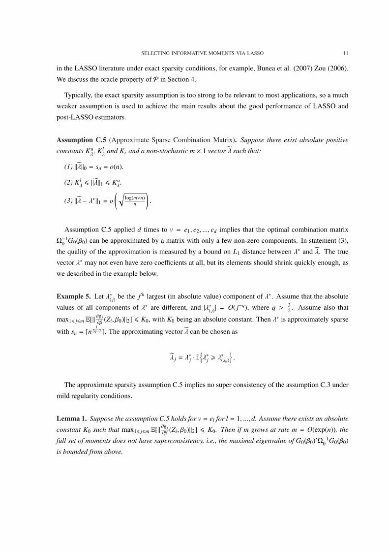
T 1. Comparison of βL and βPL with other estimators on the key parameter β1.

Number of simulations = 500.

So ||G0 j||2 is decaying with polynomial speed O( j−a). We perform the selectio procedure P with g.

The initial value of GMM estimation procedures is all set at (0.5,−1.5). We demonstrate the perfor-

mance of our selection procedure about the key parameter β1 in Tables 1, 2 and Figures 1-3. In Table

1, it is clear that βL and βPL are more efficient compared to efficient GMM and equally weighted GMM

(EW-GMM later). In addition, the bias of LASSO and the post-LASSO estimators are much smaller.

CUE has small bias when n = 400 but it is more dispersed because of its heavy tails, as such phenome-

non is discussed in Hausman et al. (2007). In Table 2, we can see that the average number of moments

selected when n = 400 is larger than that when n = 200. When sample size is smaller, the penalties

are larger and thus less moments are selected via LASSO. In our example, Algorithm 2 runs iteratively

for less than 15 times on average before it hits the stopping criteria, as described in the second row

of Table 2. Figure 1 illustrates the frequencies of moment conditions selected by the T as described

in Lemma 2. As we can observe in Figure 1, the moments picked by the selector T includes the first

a few ones and the last one, which is expected to be a strongly informative moment condition and can

be hardly picked by traditional methods such as AIC and BIC procedures proposed in Andrews (1999).

In addition, our procedure does not rely on perfect selection: the 4th moment condition is only used

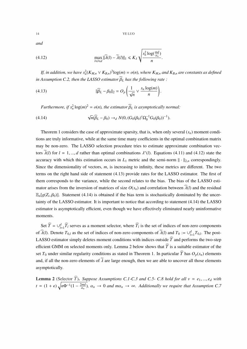
in 65% of the time when n = 200 and 25% of the time when n = 400. Figure 2-3 confirm asymptotic

normality of βL and βPL.

8 When n = 200 < m = 240, we use Ω + Im/√

n instead of Ω.

26 YE LUO

m=240 n=400 n=200

LASSO LASSO

Average number of moments selected 5.76 4.79

Average number of iteration (Algorithm 2) 14.2 12.3

Average running time per instance 15.56sec 13.52sec

T 2. More details on performance of LASSO and post-LASSO.

The next Monte-Carlo experiment is based on example 3 of Hausman, Lewis, Menzel and Newey

(2007). This example considers a Generalized-IV model when the ”second stage regression” contains

non-linear functions of the parameter β.

Example 7 (Approximate Sparse Design 2). Consider the following setting:

y = exp(xβ0) + ε,

x = zΠ + v.

We slightly modify the assumptions in Hausman, Lewis, Menzel and Newey (2007): First, x is two

dimensional, not one; Second, the number of instruments, m, is larger than the sample size, n. The true

beta β0 = (0, 0). Let m = 500 and n = 200. v ∼ N(0, 1), z1, ..., zm ∼ N(0, 1) and they are independent,

Π(1, j) = 1/ ja +1/(m+1− j)a, Π(2, j) = 1/(m/2+1/2− j)a, and ε = ρw1 +√

1 − ρ2φw2 · (∑mj=1 z j/ j)+√

1 − φ2w3, where a = 1 and w1,w2,w3 are independent standard normal random variables. The

preliminary estimate is set as the equally weighted GMM (EWGMM) estimator.

In this setting, traditional GMM and CUE estimators do not exist. We compare our estimator with

the performance of EWGMM estimator in Table 3. In table 3, though EWGMM estimator seems to

be quite close to the true parameter, but its bias to too large and lead to incorrect inference. Such bias

will lead to even worse rejection rate when n increases. Also in table 3, our LASSO and post-LASSO

estimators are nearly efficient compared to the efficiency bound (G0(β0)Ω−10 G0(β0))−1, although on

average 10.3 out of 500 moments are selected. The empirical variance of EW. The asymptotic test of

LASSO and post-LASSO estimators have the size which are slightly larger than 0.05. This is perhaps

due to the randomness of the moment selector T . In Table 1, we also see the similar phenomenon

in LASSO and post-LASSO estimators when n = 200. Again, similar to the previous Monte-Carlo

example, post-LASSO is slightly better than LASSO in MSE. Figure 4 presents the frequencies of


F 1. Frequencies of Moments Selected: Top: n = 200; Bottom: n = 400

moments which are picked by the LASSO selector. According to our design, we should expect three

groups clustered around 1, 250, and 500. We can observe exactly the same phenomenon in Figure 4.

28 YE LUO

F 2. Distribution of β1L and β2L. Top: n = 200; Bottom: n = 400.

7. C

This paper applies the LASSO method to solve the many moments problem. Instead of implementing

traditional optimal GMM with the full set of moments, we consider selecting the informative moments

before conducting the traditional optimal GMM procedure. Since the optimal GMM estimator can be

obtained via the optimal combination matrix G0(β0)′Ω−10 , we formulate a quadrative objective function

with LASSO type penalties to estimate the rows in the optimal combination matrix (d rows in total).

This method has several advantages compare to the traditional optimal GMM or GEL when the number

of moments is comparable to the sample size or even much larger than the sample size. When approx-

imate sparisty holds, first of all, our method can substantially reduce any second order bias simply

because most of the informative moments are dropped by the selection procedure; second, our method

is computationally tractable compared to other moment selection procedures such as those proposed in

Donald, Imbens and Newey (2008).

Theoretically, we establish the asymptotic bounds of the LASSO estimator of the optimal combi-

nation matrix under L1 distance and semi-norm || · ||2. Based on these bounds, we are able to prove


F 3. Distribution of β1PL and β2PL. Top: n = 200; Bottom: n = 400.

F 4. Frequencies of Moments Selected: Approximate Sparse Design 2

30 YE LUO

m=500 n=200

Bias√

nVar MSE Rej. Rate

LASSO (0.0123,−0.0005)

0.582 0.011

0.011 0.147

(3.11, 0.75) × 10−3 0.060

post-LASSO (0.0166, 0.0034)

0.524 0.006

0.006 0.145

(2.92, 0.73) × 10−3 0.060

EW-GMM (0.0559, 0.0174)

0.392 −0.016

−0.016 0.137

(5.09, 0.98) × 10−3 0.248

Eff. Bound NA

0.477 −0.060

−0.060 0.123

NA NA

Average # of Moments Chosen 10.3

T 3. Comparison of βL and βPL with equally weighted GMM estimator. Number

of simulations = 500.

consistency and establish bounds for the LASSO based GMM estimator βL and post-LASSO based

GMM-estimator βPL. Furthermore, when the number of truly informative moments, sn (as defined in

the approximate sparsity assumption), grows with speed s2n log(m)2

n → 0, we can prove that together with

a set of high-level conditions, both βL and βPL are asymptotically normal and nearly efficient. These

high-level assumptions are common in the LASSO literature. We establish primitive conditions for the

high-level assumptions such that the validity of these assumptions mainly relies on a set of growth con-

ditions for the parameters KG,n,KM,n,KB,n (which characterizes the behavior of the tail of the residuals

and the smoothness of the moment conditions) and ρ (which characterizes the accuracy of the prelim-

inary estimator). All these results are novel in dealing with non-linearity when the LASSO method is

applied.

In addition to these theoretical results, we propose a set of feasible and valid penalties to imple-

ment the LASSO procedure. Due to the complexity of our problem, our penalty terms depend on the

target of estimation, which is one of the main challenges we encounter. Such a challenge does not

arise when traditional LASSO is applied to OLS and 2SLS. We propose adaptive algorithms to solve

this difficulty that are computationally tractable. Our algorithm 1 converges globally, which guarantees

the performance of the algorithm with fast speed. Our algorithm 2 is more general and works well in


Monte-Carlo experiments, though the theoretical convergence speed is not yet known. We prove that

the convergence points in our algorithms satisfy the same properties as if we were using the penal-

ties constructed from the true parameter. The excellent performance of these adaptive algorithms is

demonstrated in Monte-Carlo experiments.

8. A A: P S 4

Proof of Lemma 1.

By assumption, for any v ∈ Rd, ||v||2 = 1, ||G0(β0)v||∞ 6 K0. If m = O(exp(n)), by statement (2) and (4)

of C.5, ||λ∗||1 6 Kuλ + o(

√log(m)

n ) is bounded from the above.

Thus, vG0(β0)′Ω−10 G0(β0)v = (λ∗)′G0(β0)v 6 ||λ∗||1||G0(β0)v||∞ 6 K0||λ∗||1 is bounded from the

above. That is to say, the maximal eigenvalue of G0(β0)′Ω−10 G0(β0) is bounded from the above.

Proof of Theorem 1.

To prove Theorem 1, I follow the strategy in BCCH (2012). The proof of this theorem is divided

into three steps. The first step provides proof for (4.11) and (4.12). The second step provides proof for

consistency of βL. The third step proves (4.13) and (4.14).

Step 1: In this step, we establish bounds for λ(l) − λ(l), 1 6 l 6 m.

For any vector x ∈ Rm, define norm || · ||1,n of x as ||x||1,n :=∑

16 j6m |x j||γ j|, and define semi-norm

|| · ||2,n of x as x′Ωx. For any c > 0 and set T ⊂ 1, 2, ...,m, define the following quantities:

(8.29) κ2c(T ) := min

||δTc ||16c||δT ||1,δ,0

s||δ||22,n||δT ||21

,

(8.30) κ2c,n(T ) := min

||δTc ||1,n6c||δT ||1,δ,0

s||δ||22,n||δT ||21,n

,

where s = |T |.

Lemma 3 of Bickel, Ritov and Tsybakov (2009) proves that bounds on κ(s, Ω) imply a lower bound

for κc(T ) and κc,n(T ). More specifically, for any positive integer s1, Bickel, Ritov and Tsybakov (2009)

shows that κc(T )2 > κ(s1, Ω)(1 − ε√

s φ(s1,Ω)s1 κ(s1,Ω)

). For s 6 sn and s1 = s log(n), the Assumption C.6

implies that

κc(T )2 > κ1

(1 − ε

√κ2

log(n)κ1

),

which is bounded from below away from 0 as n approaches infinity. So κc,n(T )2 > a2

b2 κc(T )

32 YE LUO

> a2

b2 κ1

(1 − ε

√κ2

log(n)κ1

), which verifies that κc,n(T )2 is bounded from below if s 6 sn.

Let δ := λ − λ. For λ, let T be the set of indices of non-zero components of λ. Below I establish

non-asymptotic bounds for the solution to P.

Lemma 12 (Bounds for LASSO Selector λ). Given v ∈ Rd, suppose λ is the sparse vector to be

estimated and λ is the solution to the convex optimization problem P. Let T be the set of indices of

non-zero components in λ. Assume that conditions C.1-C.3 and C.6-C.8 hold. Denote ε = ε+2ε Then,

with probability at lease 1 − αn,

(8.31) ||δ||1,n 6 ε||δT ||1,n,

and

(8.32) ||δ||2,n 6√

s2t0(2 + ε)nκε,n(T )

.

Proof. By definition, λ is the minimizer of the problem P. Therefore, tn (||δT ||1,n − ||δT c ||1,n) > Q(λ) −

Q(λ).

Meanwhile, Q(λ) − Q(λ) can be decomposed as:

(8.33) Q(λ) − Q(λ) =12δ′Ωδ − δ′Ωλ + v′G′δ >

12δ′Ωδ − ||S (λ)||∞||δ||1.

By Assumption C.7, P( t0n > max16 j6m | S j (λ)

γ j|) > 1 − αn.

By inequality (8.33), tn ||λ||1,n − t

n ||λ||1,n > |Q(λ) − Q(λ)| > ||S ||∞||δ||1 > − t0n ||δ||1,n. By setting t =

(1 + ε)t0, we know that (1 + ε)||δT ||1,n − (1 + ε)||δT c || > −||δT ||1,n − ||δT c ||1,n. Thus,

||δT c ||1,n 6 ε||δT ||1,n.

Restarting with (8.33), again tn (||δT ||1,n − ||δT c ||1,n) > 1

2 ||δ||22,n − t0n ||δT ||1,n − t0

n ||δT c ||1,n.

Therefore, 12 ||δ||22,n 6 t0(2+ε)

n ||δT ||1,n − tεn ||δT c ||1,n 6 t0(2+ε)

√s

nκε,n(T ) ||δ||2,n. Thus,

||δ||2,n 6 2t0(2 + ε)√

snκε,n(T )

.

In the Lemma 12, I establish bounds for λ−λ given a vector v ∈ Rd. To obtain a just identified system

of moment conditions, we can consider repeating the selection procedure (4.11) for v = e1, e2, ..., ed.

Define δ(l) := λ(l) − λ(l), T0,l = j|λ(l) j , 0 and T0 := ∪16l6dT0,l.


For any 1 6 l 6 d, by Lemma 12, ||δ(l)||2,n 6 2t0(2+ε)√

snnκε,n(T0) . Also, t0 = Φ−1(1 − αn

4md ) 6√

log( 4mdαn

).

Combining these inequalities, we immediately obtain (4.12):

maxl6l6d||δ(l)||2,n 6 K′λ

√sn log( 4md

αn)

n,

where K′λ := 2(2+ε)κε,n(T0) .

For (4.11), by conclusions in Lemma 12, ||δT c(l)||1,n 6 ε||δT (l)||1,n. Therefore ||δ(l)||1 6 ba ||δ(l)||1,n 6

ba

√sn

κε,n||δ(l)||2,n. The inequality (4.12) holds with constant Kλ = b

aκε,nK′λ.

Step 2: In this step, we prove consistency of βL.

Let Λ = (λ(1), λ(2), ..., λ(d)), Λ = (λ(1), λ(2), ..., λ(d)) and ∆ = (δ(1)′, δ(2)′, ..., δ(d)). By definition

∆ = Λ − Λ.

The GMM estimator βL has the following property:

(8.34) Λ′En[g(Zi, βL)] = 0.

We prove that βL is consistent. Let

qn(β) =

d∑

l=1

(λ(l)′En[g(Zi, β)])2,

qn(β) =

d∑

l=1

(λ(l)′En[g(Zi, β)])2,

qn,0(β) =

d∑

l=1

(λ(l)′E[g(Zi, β)])2,

and

q∗n(β) =

d∑

l=1

(λ∗(l)′E[g(Zi, β)])2

Consider the following decomposition:

(8.35) qn(β) − qn,0(β) = qn(β) − qn(β) + qn(β) − qn,0(β).

For the first term qn(β) − qn(β) of (8.35) can be bounded as follows:

(8.36) |qn(β)−qn(β)| 6 |d∑

l=1

En[(λ(l)−λ(l))′g(Zi, β)2]|+2|d∑

l=1

En[(λ(l)−λ(l))′g(Zi, β)λ(l)g(Zi, β)]|.

In (8.36), the important component |(λ(l)−λ(l))g(Zi, β)| goes to 0 since ‖λ(l)−λ(l)‖1 → 0 fast enough.

More specifically, |(λ(l) − λ(l))′g(Zi, β)| 6 |(λ(l) − λ(l))′g(Zi, β0)| + KM,n‖(λ(l) − λ(l))‖1 · ‖β − β0‖2. By

34 YE LUO

Holder’s inequality, |(λ(l) − λ(l))′g(Zi, β0)| 6 ‖λ(l) − λ(l)‖1 max16 j6m |g j(Zi, β0)| = Op

(√s2

n log(m)n KB,n

).

And KM,n‖(λ(l) − λ(l))′‖1 · ‖β − β0‖2 6 KM,nd(Θ), where d(Θ) is the diameter of Θ which is a finite

constant. So KM,n‖(λ(l) − λ(l))′‖1 · ‖β − β0‖2 = Op(√

s2n log(m)

n KM,n).

Therefore, |(λ(l) − λ(l))′g(Zi, β)| = Op

((KB,n ∨ KM,n)

√s2

n log(m)n

).

Using the bounds obtained above for |(λ(l) − λ(l))g(Zi, β)|, in (8.36), the fist component can be

bounded by:

|d∑

l=1

En[(λ(l) − λ(l))′g(Zi, β)2]| = Op

((KB,n ∨ KM,n)2 s2

n log(m)n

);

The second component can be bounded by:

2|d∑

l=1

En[(λ(l) − λ(l))′g(Zi, β)λ(l)′g(Zi, β)]| 6 2|d∑

l=1

| max16i6n

|(λ(l) − λ(l))′g(Zi, β)|En[|λ(l)′g(Zi, β)|]|,

where En[|λ(l)′g(Zi, β)|] 6 En[|λ(l)′g(Zi, β0)|] + ‖λ(l)‖1d(Θ)KM,n.

By statement (4) of Assumption C.2,

En[|λ(l)′g(Zi, β0)|] =∑

16 j6m

|λ(l)) j| · |En[|g j(Zi, β0)|] 6∑

16 j6m

|λ(l)) j||En[|g j(Zi, β0)|2] 6 K‖λ(l)‖1.

Therefore,

2|d∑

l=1

| max16i6n

|(λ(l) − λ(l))′g(Zi, β)|En[|λ(l)′g(Zi, β)|]| = Op

KM,n

√s2

n log(m)n

.

Combining the bounds obtained above,

qn(β) − qn(β) = Op

(KB,n ∨ KM,n)

√s2

n log(m)n

,

for any β ∈ Θ.

For the second component qn(β)−qn,0(β) in (8.35), we need to apply the ULLN for arrays. The state-

ment (1) of Assumption C.2 implies that for any β and β′ ∈ Θ, |λ′g(Z, β) − λ′g(Z, β′)| 6 ‖λ‖1K(Z)||β −β′||2, where E[‖λ‖1K(Z)] 6 KKu

λ < ∞. So by ULLN for arrays,

max16l6d

|En[λg(Z, β)] − E[λg(Z, β)]| →p 0

uniformly for any β ∈ Θ.


Thus, |qn(β)−qn,0(β)| →p 0 uniformly =for β ∈ Θ. So by construction qn,0(βL)→p 0, since qn(βL) =

0 and (KB,n ∨ KM,n)√

s2n log(m)

n →p 0. In addition, by Assumption C.5, ‖λ(l) − λ∗(l)‖1 = o(√

log(m)n ), for

all 1 6 l 6 d. Hence,

|λ(l)′E[g(Z, β)]−λ∗(l)E[g(Z, β)]| = |(λ(l)−λ∗(l))′E[g(Z, β)]−E[g(Z, β0)] 6 ||λ(l)−λ∗(l)||1d(Θ)E[KM(Z)].

So by assumption that log(m)3

n → 0, q∗n(β) − qn,0(β) → 0 uniformly in β ∈ Θ. Hence, q∗n(βL) →p 0. It

follows immediately that together with statement (5) of Assumption C.2, ‖βL − β0‖2 →p 0.

Step 3: In this step, we prove asymptotic properties of βL.

By Assumption C.2, the local expansion can be expanded as:

(8.37) −Λ′En[g(Zi, β0)] = Λ′En[g(Zi, βL)] − En[g(Zi, β0)]

On the left hand side of (8.37),

(8.38) Λ′En[g(Zi, β0)] = Λ′En[g(Zi, β0)] + (Λ − Λ)′En[g(Zi, β0)].

By Assumption C.2 and C.4, the first component of (8.38) consists the mean of a d×1 random vector

with bounded variance. So by the array Linderberg Feller Central limit theorem,√

nΛ′En[g(Zi, β0)]→d N(0, Λ′Ω0Λ),

where Λ′Ω0Λ = (G0(β0)′Ω−10 G0(β0))−1 + o(

√log(m)

n ), which is nearly efficient.

The second component of (8.38) consists the bias comming from the correlation of the estimated

optimal combination matrix Λ and En[g(Zi, β0)]. By (4.12), for all 1 6 l 6 d, with probability increasing

to one, ||λ(l) − λ(l)||1 6 K′λ

√s2

n log(4m/αn)n .

To obtain an upper bound for max16 j6m En[g(Zi, β0)], we need to use the moderate-deviation theory

of self-normalized vectors. For detailed theory and bounds, we refer to Shao and Zhou (2003) and De

La Pena et. al.(2009). If statement (3) of Assumption C.2 holds, Lemma 5 of BCCH provides a useful

result to bound max16 j6m En[g(Zi, β0)].

Lemma 13. Suppose that for each 1 6 j 6 m, R j :=∑

16 j6m U j√∑16 j6m U2

j

, where Ui j are independent random

variables across i with mean 0. If E[|Ui j|3] - 1, then with log(m)n1/3 → 0, there exists a sequence ln → ∞

such that for any α small enough,

(8.39) P( max16 j6m

|R j| 6 Φ−1(1 − α

2m)) > 1 − α(1 +

Aln

),

where A is an absolute constant.

36 YE LUO

Hence, apply Lemma 13 to our problem, with probability increasing to one, |max16 j6m En[g j(Zi, β0)]| 6Φ−1(1− 2m

αn)

n

√max16 j6m En[|g j(Zi, β0)|2] = O(

√log(m)

n ). Therefore, the second component of (8.38) can be

bounded by:

|(λ(l)−λ(l))′En[g j(Zi, β0)]| 6 ||(λ(l)−λ(l))||1 max16 j6m

|En[g j(Zi, β0)]| 6p C

√s2

n log(m)n

√log(m)

n= C

sn log(m)n

,

with C being some generic constant.

On the right hand side of (8.37), we have the following decomposition:

(8.40) ΛEn[g(Z, βL)] − En[g(Z, β0)] = En[Λg(Z, βL)] − En[Λg(Z, β0)]

+(Λ − Λ)En[g(Z, βL)] − En[g(Z, β0)].For the first component of (8.40), En[Λg(Z, βL)] − En[Λg(Z, β0)] = En[Λ ∂g

∂β (Z, β∗)](βL − β0) for some

β∗ = β0 + O(||βL − β0||2).

We consider apply ULLN to ∂g∂β (Z, β∗). Let Fn := ∂g

∂β (Z, β) − ∂g∂β (Z, β0)|β ∈ Θ be a class of functions

indicated by elements in Θ. So | ∂g∂β (Z, β) − ∂g

∂β (Z, β0)| 6 KG(Z)d(Θ)Kuλ . By statement (1) of Assumption

C.2, E[KG(Z)] 6 K, so the ULLN for arrays holds:

limn→∞ sup

f∈Fn

||En[ f (Z)] − E[ f (Z)]||2 → 0 almost surely.

Therefore, En[Λ′g(Z, βL)] − En[Λ′g(Z, β0)] = (Λ′G0(β0) + op(1))(βL − β0).

For the second component of (8.40),

(Λ − Λ)En[g(Z, βL)] − En[g(Z, β0)] 6 max16l6d

||λ(l) − λ(l)||1KM,n||βL − β0||2 = Op(KM,n

√s2

n log(m)n

).

By assumption, KM,n

√s2

n log(m)n →p 0, so the right hand side of (8.37) can be written as:

(Λ′G0(β0) + op(1))(βL − β0).

It is also easy to verify that by statement (3) of Assumption C.5, Λ′G0(β0) = G0(β0)Ω−10 G0(β0) +

o(√

log(m)n ).

Combining the asymptotic approximation of two sides in (8.37), we get:

||βL − β0||2 = Op

(1√n∨ s0log(m)

n

).

In addition, ifs2

0 log(m)2

n = o(1), then s0log(m)n = o( 1√

n). Therefore,

(8.41)√

n(βL − β0)→d N(0,Vn),


with Vn − (G0(β0)′Ω−10 G0(β0))−1 → 0.

Proof of Lemma 2.

Here we need a set of results similar to Lemma 7-Lemma 9 stated in BCCH. For any l = 1, 2, ..., d, we

define m = |TlTl|, where Tl is the set of indices of non-zero components in λ(l). We need to prove

that m = Op(sn). In fact we only need to prove that m = Op(|Tl|).

Notice that the first order condition gives:

S (λ(l)) j = sign(λ) jγ jtn,

for any j ∈ TlTl. For simplicity, for two vectors A and B with same length, we let AB := ( A j

B j) j>1.

Therefore,

(8.42) (1 + ε)t0n

√ml = || S (λ)

γ TlTl

||2 6 || S (λ(l))γ TlTl

||2 + ||Ω(λ(l) − λ(l))γ TlTl

||2.

The first component of the above expression is bounded by:

|| S (λ(l))γ TlTl

||2 6√

mlt0n,

with probability at least 1 − αn − εn.

For the second term,

||Ω(λ(l) − λ(l))γ TlTl

||2 6 1a||Ω(λ(l) − λ(l)TlTl

||2.

Define UTl = Tl ∪ Tl.

For any j ∈ TlTl, Ω(λ(l) − λ(l) j :=∑

j∈UTlΩ jk (λ(l)k − λ(l)k). Therefore, Ω(λ(l) − λ(l))TlTl

=

ΩUTl (λ(l)UTl − λ(l)UTl)TlTl, which only depends on the subset UTl with size at most ml + sn.

Next, we need a simple fact from Lemma 9 of BCCH. Namely, the function φ(s,M) is sub-additive,

i.e., φ(s1,M) + φ(s2,M) > φ(s1 + s2,M), for s1 and s2 being positive integers. This implies that for any

real number q > 1 and positive integer s, φ(dsq,Me) 6 dqeφ(s,M).

||Ω(λ(l) − λ(l))TlTl||2 6 ||ΩUTl (λ(l)UTl − λ(l)UTl)||2 = ||Ω

12UTl

(λ(l)UTl − λ(l)UTl)||2,n.

We know that ||Ω12UTl

(λ(l)UTl − λ(l)UTl)||2 = ||λ(l)UTl − λ(l)UTl ||2,n 6 Kλ

√sntn with probability at least

1−αn − εn (in fact this result holds at the same events when || S (λ(l))γ TlTl

||2 6√

mlt0n , therefore we don’t

38 YE LUO

need to correct the size of the probability to let both situation hold simultaneously). Therefore,

||Ω(λ(l) − λ(l))TlTl||2 6 ||ΩUTl (λ(l)UTl − λ(l)UTl)||2 6

√snKλtan

√φ(sn + ml, Ω).

Combining the bounds we obtained above, we get the following bounds as we review (8.42):

εt0n

√ml 6

√snKλtan

√φ(sn + ml, Ω).

Consequently, ml 6 sn( Kλ(1+ε)aε )2

√φ(sn + ml, Ω). Denote C0 := ( Kλ(1+ε)

aε )2κ2. Let C∗ be an abso-

lute constant > 2C0. Let p∗ = C∗sn. Therefore, φ(dp∗e, Ω) 6 κ2 as n → ∞, as we assume that

φ(sn log(n), Ω) 6 κ2. Therefore, ml 6 C0snφ(dp∗e, Ω)d sn+mlC∗sne 6 C0snκ2(1 +

sn+mlC∗sn

) 6 C0snκ2 +sn+ml

2 .

Hence, ml 6 (2C0κ2 + 1)sn.

Step (2) is derived based on results stated in (4.12). It is quite obvious that λ(l) j is non-zero if j ∈ Tl

when the assumption√


n log(m)→ ∞ holds.

Proof of Theorem 2.

Based on Lemma 2, we have that |T | 6 Csn for some absolute constant C with probability at least

1 − αn − εn. So ΩT has eigenvalues bounded from above and away from 0.

Consider λT (l) := Ω−1T

G(β)el. Therefore Q(λT ) 6 Q(λ(l)) by construction. Denote δT (l) := λT (l) −λ(l). Therefore,

12δT (l)′ΩδT (l) 6 −δT (l)′S (λ(l)) = −δT (l)′S (λl) − δT (l)′Ω(λ(l) − λ(l)).

By the fact that ||δT ||0 6 Csn and Assumption C.7, for the first component −δT (l)′S (λl), we have

| − δT (l)′S (λl)| 6 tn||δT (l)||1,n 6 bt

√Csn

nκ1||δT (l)||2,n.

For the second component, δT (l)′Ω(λ(l) − λ(l)), we have

|δT (l)′Ω(λ(l) − λ(l))| 6 ||δT (l)||2,n||λ(l) − λ(l)||2,n 6 Kλ

t√

sn

n||δT (l)||2,n.

The two bounds above implies that ||δT (l)||2,n 6 K(l) t√

snn , where K(l) := 2( b

√C

κ1+ Kλ) is an absolute

constant. Therefore, it follows that ||λT (l) − λ(l)||2,n 6 (K(l) + Kλ) t√

snn .

It follows that

||λT (l) − λ(l)||2 6||λT (l) − λ(l)||2,nκ(ml + sn, Ω)

6(K(l) + Kλ)

κ1

t√

sn

n,


and by Cauchy-Schwarz inequality

||λT (l) − λ(l)||1 6√

ml + sn||λT (l) − λ(l)||2 6 (K(l) + Kλ)√

C + 1κ1

tsn

n.

So we have established similar bounds for λT (l) − λ(l) as we did for λ(l) − λ(l) in Theorem 1.

Since all the arguments in step 2 and step 3 in Theorem 1 can be carried over to this theorem, based

on λT (l)−λ(l) instead of λ(l)−λ(l), so the conclusion stated in Theorem 2 holds due to similar argument

illustrated in the proof of Theorem 1.

Proof of Corollary 1. This results is based on the fact that T0 ⊂ T and |T | = O(sn) with probability at

least 1 − αn − εn. The derivation is similar to Step 2 and 3 in Theorem 1 except that we do not pay

additional log(m) is the bounds stated in (4.13). I abbreviate the proof here.

9. A B: P S 5

Proof of Lemma 4.

Denote wi = g(Zi, β) − g(Zi, β0). By Assumption C.2, max16 j6m |wi j| 6 KG,n||β − β||2.

Consider the sparse eigenvalue of Ω = En[g(Zi, β)g(Zi, β)′]. We compare Ω with Ω0 = En[g(Zi, β0)g(Zi, β0)′].For any ||δ||2 = 1 and ||δ||0 6 sn log(n),

(9.43) δ′Ωδ − δ′Ω0δ = 2En[(δ′wi)(g(Zi, β0)′δ)] + En[(δ′wi)2].

By Cauchy-Schwarz inequality,

|En[(δ′wi)(g(Zi, β0)′δ)]| 6 En[(w′iδ)2]

12En[(g(Zi, β0)′δ)2]

12 6 φ(sn log(n), Ω0)

12En[(w′iδ)

2]12 .

By Holder-inequality with the conditions ||δ||0 6 sn log(n) and sn log(n)K2M,n = op(n2ρ),

En[(w′iδ)2] 6 En[(||wi||∞||δ||1)2] 6 En[K2

M,n||β − β0||22sn log(n)||δ||22] = K2M sn log(n)op(n−2ρ) = op(1).

Therefore,

φ(log(s)sn, Ω − Ω0) = max||δ||2=1,||δ||06sn log(n)

|δ′Ωδ − δ′Ω0δ|

6 2(K2

M sn log(n)

n2ρ )12 κ1,0 +

K2M sn log(n)

n2ρ →p 0.

If in addition Assumption C.9 holds that: κ1 6 κ(Cs, Ω0) 6 φ(Cs, Ω0) 6 κ2, for any δ on the unit sphere

and ||δ0|| 6 Cs0,

δ′Ωδ = δ′Ω0δ + (δ′Ωδ − δ′Ω0δ) = δ′Ω0δ + op(1).

40 YE LUO

Let c be a small absolute constant such that c < κ1,02 . So with probability going to one, 0 < κ1,0 − c 6

κ(sn log(n), Ω) 6 φ(sn log(n), Ω) 6 κ2,0 + c.

Proof of Lemma 5.

The score of objective function Q at λ can be expanded as: S (λ) = (Ω−Ω0)λ− (G(β)−G0(β0))+Ω0(λ−λ∗). Let T be the set of indices of non-zero components of λ. Therefore, for each j ∈ 1, 2, ...,m,

(9.44) S j =∑

k∈Tλk(En[g j(Zi, β)gk(Zi, β)]−E[g j(Zi, β0)gk(Zi, β0)])−(En[

∂g j

∂β(Zi, β)v]−E[

∂g j

∂β(Zi, β0)v])

+∑

16k6m

Ω0, jk (λk − λ∗k).

There are three components in the above equation 9.44):

(1)∑

k∈T λk(En[g j(Zi, β)gk(Zi, β)] − E[g j(Zi, β0)gk(Zi, β0)]);

(2) En[∂g j∂β (Zi, β)v] − E[∂g j

∂β (Zi, β0)v];

(3)∑

16k6m Ω0, jk (λk − λ∗k).

Step 1: Consider the upper bound of the first component in equation (9.44). Obviously,

(9.45) ||(Ω −Ω0)λ||∞ 6 ||(Ω − Ω0)λ||∞ + ||(Ω0 −Ω0)λ||∞.

The first part of the decomposition (9.45) is ||(Ω − Ω0)λ||∞.

Similar to the calculation in Lemma 4, we could prove that:

||(Ω − Ω0)λ||∞ is bounded by:

||(Ω − Ω0)λ||∞ 6 ||(Ω − Ω0)||∞||λ||1 6p (1 + ε)2KM,n||β − β0||2||λ||1,where 1 > c > 0 be a small absolute constant and ||(Ω − Ω0)||∞ := max16 j6m,16k6m |Ω jk − Ω0, jk|.

The second part of the decomposition (9.45) is ||(Ω0 − Ω0)λ||∞. To obtain an upper bound for this

term, again we need to use the moderate-deviation theory from Lemma 13.

By assumption (g(Zi, β0)g(Zi, β0)′ −Ω0)λ j are independent random variables across i with mean 0.

It is easy to show that E[|(g(Zi, β0)g(Zi, β0)′ − Ω0)λ j|3] 6 max16 j6m E[|g j(Zi, β0)6|]||λ||31 6 Kug (Ku

λ)3 <

∞. Thus, for n large enough, there exists a term qn := Aln→ 0 such that Pr(|(Ω0 − Ω0)λ j| <

En[((g(Zi, β0)g(Zi, β0) −Ω0)′λ)2j]Φ−1(1 − α

4m ), for all1 6 j 6 m) > 1 − α(1 + qn).

However, En[((g(Zi, β0)g(Zi, β0)′−Ω0)λ j)2] can not be used in practice to bound |(Ω0−Ω0)λ j| be-

cause Ω0 is unknown. Instead, we establish bounds using the empirical variance En[((g(Zi, β0)g(Zi, β0)′−Ω0)λ j)2]. Let Ui j be (g(Zi, β0)g(Zi, β0)′−Ω0)λ j. Denote U = En[U]. We apply a modified version of


Lemma 13 to bound max16 j6m U j. Let z j = U

En[((g(Zi,β0)g(Zi,β0)′−Ω0 )λ j)2] 12

be the infeasible Z− statistic.

Lemma 13 establishes bounds for the Z− statistic.

Consider the t-statistic t j :=√

n U jsu j

, where su j := S e(U j) := 1n−1

∑16 j6m(U j − U)2 1

2 . Notice that

there is a simple relationship between t j and z j:

t j := z j

√n − 1n − z2

j

.

Thus, P(t j > x) = P(z j > x( nn+x2−1 )

12 ) for any x. Let x = Φ−1(1 − α

4m ), so by assumption x3 =

O(log(m)3) = o(n). Therefore, P(t j > x) = P(z j > x( nn+x2−1 )

12 ) > (1−η)P(z j > Φ−1(1− α

4m )) > 1− α2 −η

as n→ ∞ for any small number η > 0.

Now replace Ui j with (g(Zi, β0)g(Zi, β0)′ −Ω0)λ j. So

nn − 1

su2j = En[(

m∑

k=1

gk(Zi, β0)g j(Zi, β0)λk)2] − [En(m∑

k=1

gk(Zi, β0)g j(Zi, β0)λk)]2.

Therefore, Pr( √

n|((Ω0−Ω0 )λ) j |En[(

∑mk=1 gk(Zi,β0)g j(Zi,β0 )λk)2]−En[

∑mk=1 gk(Zi,β0)g j(Zi,β0 )λk]2 1

26 Φ−1(1 − α

4m ), for all 1 6 j 6 m)>

1 − αn2 + o(1).

(2) The second component in (9.44) can be decomposed as:

(9.46) En[∂g j

∂β(Zi, β)v] − E[

∂g j

∂β(Zi, β0)v] = (En[(

∂g j

∂β(Zi, β)v)] − En[(

∂g j

∂β(Zi, β0)v)])

+(En[(∂g j

∂β(Zi, β0)v)] − E[(

∂g j

∂β(Zi, β0)v)]).

By Lemma 3, the first part of (9.46) is bounded by KG ||β − β0||2. The second part of (9.46) can

be bounded by En[|∂g j∂β (Zi, β0)|2] − En[∂g j

∂β (Zi, β0)]2 using the same strategy as described in the previous

component. Thus, Pr(√

n|En[

∂g j∂β (Zi,β0)v]−E[

∂g j∂β (Zi,β0)v]|

En[(∂g j∂β (Zi,β0)v)2]−[En(

∂g j∂β (Zi,β0)v)]2 1

26 Φ−1(1 − α

4m ), for all 1 6 j 6 m) > 1 − αn2 +

o(1).

(3) The third component Ω0(λ−λ∗) is non-stochastic constant. It equals to 0 if λ∗ obeys exact sparse

assumption C.4.

The penalty γ j proposed in Lemma 5 is a combination of the upper bounds described in steps (a),

(b) and (c). Hence,

(9.47) P( max16 j6m

∣∣∣∣∣∣∣S j(λ)γ j

∣∣∣∣∣∣∣ 6 Φ−1(1 − αn

4m)) > 1 − αn + o(1).

42 YE LUO

Proof of Corollary 2. By Assumption C.5, we know that ||λ − λ∗||1 = op(√

mn ). Therefore, ‖Ω0(λ −

λ∗)‖ →p 0. If (KG,n∨KM,n)2

n2ρ−1 log(m) → 0, the first term stated in 5.15 would also converge to 0. Hence, if

assumption C.8 holds, the penalties γRj is uniformly converging to the infeasible penalties γ j stated in

Lemma 5, for all 1 6 j 6 m.

Hence, there exists a sequence ε′n → 0 such that with probability at least 1 − αn − εn − ε′n,

max16 j6m

∣∣∣∣∣∣∣S j(λ)γ j

∣∣∣∣∣∣∣ 6t0n.

Proof of Lemma 6. Lemma 13 allows us to bound the maxima of a vector with length m of empirical

averages of mean zero i.i.d data. For l = 1, 2, ..., d, let γ(l) be the vector of penalties for v = el, and

S l(λ) be the score function of 12λ′Ωλ − λ′G(β)el.

To bound the maxima of∣∣∣∣∣S l (λ) jγ j(l)

∣∣∣∣∣ for all 1 6 j 6 m and 1 6 l 6 d, we can simply consider the 1 × md

vector S ∗ := (S 1(λ)′, S 2(λ)′, ..., S d (λ)′). So we can apply Lemma 13 to S ∗ and the uniform upper

bound for∣∣∣∣∣S l (λ) jγ j(l)

∣∣∣∣∣ will be√


), with probability at least 1 − αn − o(1).

Proof of Lemma 7. The proof of this Lemma is quite straight forward. Statement (2) in Assumption

C.11 guarantees that both γRj and γC

j are bounded from below by KlG, 1 6 j 6 m. Assumption C.5 and

statement (1) in Assumption C.11 guarantees that both γRj and γC

j are bounded from the above.

Proof of Lemma 8.

(1) For the refined penalty γRj , denote

wgj := En[(

∑

16k6m

gk(Zi, β)g j(Zi, β)λk)2] − [En(∑

16k6m

gk(Zi, β)g j(Zi, β)λk)]2

−En[(∑

k∈T0

gk(Zi, β0)g j(Zi, β0)λk)2] − [En(∑

k∈T0

gk(Zi, β0)g j(Zi, β0)λk)]2,

and

wGj := En[(

∂g j

∂β(Zi, β)v)2] − [En

∂g j

∂β(Zi, β)v]2 − En[

∂g j

∂β(Zi, β0)v2] − En[

∂g j

∂β(Zi, β0)v]2.

It is easy to rewrite wgj and wG

j as:

wgj = En[(

∑

16k6m

gk(Zi, β)g j(Zi, β)λk)2] − En[(∑

k∈T0

gk(Zi, β0)g j(Zi, β0)λk)2]


−[En(∑

16k6m

gk(Zi, β0)g j(Zi, β0)λk)]2 − [En(∑

k∈T0


and

wGj = En[(

∂g j

∂β(Zi, β)v)2] − En[(

∂g j

∂β(Zi, β0)v)2] − [En

∂g j

∂β(Zi, β)v]2 − [En

∂g j

∂β(Zi, β0)v]2.

First,

En[(∑

16k6m


k∈T0


= En[∑

16k6m

gk(Zi, β)g j(Zi, β)λk − gk(Zi, β0)g j(Zi, β0)λk2]

−2En[∑

16k6m

gk(Zi, β)g j(Zi, β)λk − gk(Zi, β0)g j(Zi, β0)λk2]∑

16k′6m

gk′(Zi, β0)g j(Zi, β0)λk′]

6 En[∑

16k6m

gk(Zi, β)g j(Zi, β)λk − gk(Zi, β0)g j(Zi, β0)λk2]

+2En[∑

16k6m

gk(Zi, β)g j(Zi, β)λk − gk(Zi, β0)g j(Zi, β0)λk2]12En[

∑

16k′6m

gk′(Zi, β0)g j(Zi, β0)λk′2].

The key component∑

16k6mgk(Zi, β)g j(Zi, β)λk − gk(Zi, β0)g j(Zi, β0)λk is bounded by:

∑

16k6m

∣∣∣∣gk(Zi, β)g j(Zi, β)λk − gk(Zi, β0)g j(Zi, β0)λk∣∣∣∣ 6

∣∣∣∣∣∣∣∑

16k6m

gk(Zi, β0)g j(Zi, β0)(λk − λk)

∣∣∣∣∣∣∣

+

∣∣∣∣∣∣∣∑

16k6m

gk(Zi, β)g j(Zi, β) − gk(Zi, β0)g j(Zi, β0)λk

∣∣∣∣∣∣∣6

∑

16k6m

∣∣∣gk(Zi, β0)g j(Zi, β0)∣∣∣ |λk − λk| + (2KM,n||β − β0||2 + K2

M,n||β − β0||22)||λ||21.

By assumption KM,n||β−β0||2 →p 0, so K2M,n||β−β0||22||λ||21 is smaller than KM,n||β−β0||2 as n→ ∞with

probability going to one. So there exists a small 1 > c > 0 such that 2KM,n||β − β0||2 + K2M,n||β − β0||22 6

(2 + c)KM,n||β − β0||2 with probability going to one.

Therefore, En[∑16k6m gk(Zi, β0)g j(Zi, β0)λk − gk(Zi, β0)g j(Zi, β0)λk2] 6∑

16k,k′6m En[|λk − λk||λk′ −λk′ ||gk(Zi, β0)gk′(Zi, β0)g j(Zi, β0)2|] 6 max16 j6m En[g j(Zi, β0)4]

∑16k,k′6m |λk−λk||λk′−λk′ | 6 Ku

g ||λ−λ||21.

Similarly, En[(∑

16k′6m gk′(Zi, β0)g j(Zi, β0)λk′)2] 6 Kug ||λ||21.

So by the fact that (x + y)2 6 2x2 + 2y2, we get:

En[∑

16k6m

gk(Zi, β)g j(Zi, β)λk − gk(Zi, β0)g j(Zi, β0)λk2] 6

2En[∑

16k6m

gk(Zi, β0)g j(Zi, β0)λk−gk(Zi, β0)g j(Zi, β0)λk2]+En[∑

16k6m

gk(Zi, β)g j(Zi, β)−gk(Zi, β0)g j(Zi, β0)λk2]

44 YE LUO

6 Kug ||λ − λ||21 + 2(2 + c)2K2

M,n||β − β0||22||λ||21.

By assumption, KM,n||β − β0||2 →p 0, ||λ − λ||1 →p 0, ||λ||1 6 Kuλ , therefore

wgj = En[(

∑

16k6m


k∈T0

gk(Zi, β0)g j(Zi, β0)λk)2]→p 0.

Second,

wgj = En[(

∑

16k6m


k∈T0


−[En(∑

16k6m

gk(Zi, β0)g j(Zi, β0)λk)]2 − [En(∑

k∈T0


and

wGj = En[(

∂g j

∂β(Zi, β)v)2] − En[(

∂g j

∂β(Zi, β0)v)2] − [En

∂g j

∂β(Zi, β)v]2 − [En

∂g j

∂β(Zi, β0)v]2.

Statement (1) of Assumption C.2 implies that maxi, j |(∂g j∂β (Zi, β0)v) j| 6 KM,n. Therefore,

En[(∂g j

∂β(Zi, β)v)2] − En[(

∂g j

∂β(Zi, β0)v)2] = En[(

∂g j

∂β(Zi, β)v − ∂g j

∂β(Zi, β0)v)2]

+2En[∂g j

∂β(Zi, β)v − ∂g j

∂β(Zi, β0)v∂g j

∂β(Zi, β0)v].

6 K2G ||β − β0||22 + 2En[KG(Z)]KM,n||β − β0||2.

And similarly,

[En∂g j

∂β(Zi, β)v]2 − [En

∂g j

∂β(Zi, β0)v]2| 6 K2

G ||β − β0||22 + En[KG(Z)]KM,n||β − β0||2.

By the LLN for arrays, En[KG(Z)]→p E[KG(Z)] 6 K. Therefore, by assumption KG,n||β−β0||2 →p 0

and KM,n||β − β0||2 →p 0. Thus, wGj →p 0.

Notice the upper bounds that we derived for wgj and wG

j are uniform in j, therefore wgj and wG

j

converges to 0 w.p. → 1 uniformly. Hence γRj → γR

j uniformly, i.e., there exists a constant Kγ,n → 0

such that max16 j6m |γRj − γR

j | 6 Kγ,n.

By assumption C.7, γRj is bounded from above and below. Suppose a 6 γR

j 6 b for all 1 6 j 6 m.

Therefore, 1 − Kγ,na 6γR

j

γRj6 1 +

Kγ,na .

(2) The proof is similar to the argument presented in (1). I abbreviate the proof here.


Proof of Theorem 3. In fact it is suffice to show that a similar version of Assumption C.7 holds, since

the Proof of Theorem 1 and Theorem 2 only relies on Assumption C.7 for the penalty terms together

with other technical conditions. The high level Assumptions C.6 are verified by the Assumptions C.1-

C.3, C.5, C.9-C.11 and the growing conditions (1) and (2)stated in Theorem 3.

By Lemma 8, the γR (or γC) satisfiesγR

j

γRj→ 1 uniformly for j = 1, 2, ...,m. From now on, we

only mention γR since all logics for γR can be carried over to γC . So Assumption C.8 also holds as n

approaches infinity.

Also by Lemma 8, there exists a sequence of positive numbers ε′n converging to 0 such that with

probability at least > 1 − ε′n, 11+ ε

36 γR

γRj6 1 + ε

3 , where we know that ε is a small but fixed positive

number. Therefore, since we know that with probability at least 1 − αn − εn, we have:

max16 j6m

∣∣∣∣∣∣∣|S (λ) j|γR

j

∣∣∣∣∣∣∣ 6t0n.

Then, with probability at least 1 − αn − εn − ε′n,

max16 j6m

∣∣∣∣∣∣∣S (λ) j

γRj

∣∣∣∣∣∣∣ 6t0n

(1 +ε

3).

Denote t′0 =t0n (1+ ε

3 ). So for ε < 0.2, we know that t > t′0(1+ ε2 ). Then all the derivations in Theorem

1 and Theorem 2 follows with the constants constructed with ε2 , not ε.

Proof of Lemma 9.

Suppose there are λ1 and λ2 such that ||λ1||1 6 ||λ2||1. Let λ1 = π(λ1) and λ2 = π(λ2) to be the solutions

of the problem P with penalties terms constructed by the parameters λ1 and λ2.

Denote q =max16 j6m(Eng j(Zi, β0)4 − [Eng j(Zi, β0)2]2)

12 . q is a positive real number bounded from

the above. So γCj (λ) = q||λ||1 +

En|(G(Zi, β)v) j|2 − [En(G(Zi, β)v) j]2

12 .

Consider the objective function Q(λ) = 12λ′Ωλ − λ′G(β)v.

By definition, Q(λ1)+q||λ1||1||λ1||1+En|(G(Zi, β)v) j|2 − [En(G(Zi, β)v) j]2

12 ||λ1||1 6 Q(λ2)+q||λ1||1||λ2||1+


12 ||λ2||1,

and Q(λ2) + q||λ2||1||λ2||1 +En|(G(Zi, β)v) j|2 − [En(G(Zi, β)v) j]2

12 ||λ2||1 6 Q(λ1) + q||λ2||1||λ1||1 +


12 ||λ1||1.

Adding the above two inequalities together, we obtain the following inequality:

||λ1||1||λ1||1 + ||λ2||1||λ2||1 6 ||λ2||1||λ1||1 + ||λ1||1||λ2||1.

46 YE LUO

Since we assume ||λ1||1 6 ||λ2||1, it is easy to see that ||λ1||1 > ||λ2||1. That is to say, the function

π2 : x 7→ ||π1(x)||1 is a non-negative, decreasing function mapping from [0,∞) to [0,∞). Therefore, π2

only has one unique fixed point ∈ [0,+∞), that is xC .

It is suffice to choose ξ >max16 j6m

En |(G(Zi ,β)v) j |2−[En(G(Zi ,β)v) j]2

12

q , since 0 would be the solution to Punder the penalty terms with ||λ||1 = ξ in (5.20). So the fixed point must lies between π2(x0) and π2(x1).

The binomial search algorithm finds the fixed point within logarithm time of ξη .

Proof of Lemma 10 and Lemma 11.

The proofs of Lemma 10 and Lemma 11 are based on Theorem 3. By the properties of γC and γR, it is

easy to verify that λC(l) and λR(l) are consistent estimators of λ(l) in L1 norm, for all 1 6 l 6 d:

(1) For the empirical coarse penalty γC , since we know that by Theorem 3, ||π(λ)−λ||1 = Op(√

s2n log(m)

n )

is converging to 0, then π2(||λ||1)− ||λ||1 →p 0. By Lemma 9, we know that π2 is a decreasing function.

The fixed point xC must satisfy that π2(||λ||1) 6 xC 6 ||λ||1 or ||λ||1 6 xC 6 π2(||λ||1). In both cases we

have xC − ||λ||1 →p 0. Then it follows that γ j defined by ||λ||1 = xC are valid for all 1 6 j 6 m, i.e., they

satisfy the results stated in Lemma 8. If follows that ||λC − λ||1 →p 0.

(2) For the empirical refined penalty γR, since the initial value is consistent in L1 distance, we would

have that for any p > 0, ||λ(p) − λ||1 →p 0, followed by the results stated in Theorem 3. Therefore,

||λR − λ||1 → 0.

Therefore, the corresponding penalties using λC and λR are valid, i.e., the results stated in Lemma 8

holds. Then the logic of Theorem 3 leads all results stated in Lemma 10 and Lemma 11.

R

[1] Andrews, D. W. (1999). Consistent moment selection procedures for generalized method of moments estimation. Econo-

metrica, 67(3), 543-563.

[2] Bekker, P.A., Alternative Approximations to the Distributions of Instrumental Variables Estimators, Econometrica 63,

657-681, 1994.

[3] Belloni, A., and Chernozhukov, V. (2010). Post-l1-penalized estimators in high-dimensional linear regression models

(No. CWP13/10). cemmap working paper.

[4] (a) Belloni, A., and Chernozhukov, V. (2011). High dimensional sparse econometric models: An introduction (pp.

121-156). Springer Berlin Heidelberg.

(b) Belloni, A., and Chernozhukov, V. (2011). l1-penalized quantile regression in high-dimensional sparse models. The

Annals of Statistics, 39(1), 82-130.

[5] Belloni, A., Chernozhukov, V., and Hansen, C. (2011). Inference for high-dimensional sparse econometric models.

arXiv preprint arXiv:1201.0220.


[6] Belloni, A., Chen, D., Chernozhukov, V., and Hansen, C. (2012). Sparse models and methods for optimal instruments

with an application to eminent domain. Econometrica, 80(6), 2369-2429.

[7] Bickel, P. J., Ritov, Y. A., and Tsybakov, A. B. (2009). Simultaneous analysis of Lasso and Dantzig selector. The Annals

of Statistics, 1705-1732.

[8] Bunea, F., Tsybakov, A., and Wegkamp, M. (2007). Sparsity oracle inequalities for the Lasso. Electronic Journal of

Statistics, 1, 169-194.

[9] Candes, E., and Tao, T. (2007). The Dantzig selector: Statistical estimation when p is much larger than n. The Annals

of Statistics, 2313-2351.

[10] Puna, V. H., Lai, T. L., and Shao, Q. M. (2008). Self-normalized processes: Limit theory and Statistical Applications.

Springer.

[11] Donald, S. G., Imbens, G. W., and Newey, W. K. (2003). Empirical likelihood estimation and consistent tests with

conditional moment restrictions. Journal of Econometrics, 117(1), 55-93.

[12] Donald, S. G., Imbens, G., and Newey, W. (2008). Choosing the number of moments in conditional moment restriction

models.

[13] Hansen., L, Large Sample Properties of Generalized Method of Moments Estimators, Econometrica, 1982, vol. 50, issue

4, pages 1029-54.

[14] Han, C., and Phillips, P. C. (2006). GMM with many moment conditions. Econometrica, 74(1), 147-192.

[15] Hansen, C., Hausman, J., and Newey, W. (2008). Estimation with many instrumental variables. Journal of Business and

Economic Statistics, 26(4).

[16] Hausman, J., Menzel, K., Lewis, R., and Newey, W. (2007). A reduced bias GMM-like estimator with reduced estimator

dispersion (No. CWP24/07). cemmap working paper, Centre for Microdata Methods and Practice.

[17] Huang, J., Ma, S., and Zhang, C. H. (2008). Adaptive Lasso for sparse high-dimensional regression models. Statistica

Sinica, 18(4), 1603.

[18] Jing, B. Y., Shao, Q. M., and Wang, Q. (2003). Self-normalized Cramr-type large deviations for independent random

variables. The Annals of probability, 31(4), 2167-2215.

[19] Newey, W. K., and Smith, R. J. (2004). Higher order properties of GMM and generalized empirical likelihood estimators.

Econometrica, 72(1), 219-255.

[20] Newey, W. K., and Windmeijer, F. (2009). Generalized method of moments with many weak moment conditions. Econo-

metrica, 77(3), 687-719.

[21] Rosenbaum, M., and Tsybakov, A. B. (2010). Sparse recovery under matrix uncertainty. The Annals of Statistics, 38(5),

2620-2651

[22] Shi, Z. (2013). Econometric Estimation with High-Dimensional Moment Equalities. In Meeting of the Econometric

Society in June (p. 1).

[23] Tchuente, G., and Carrasco, M. (2013). Regularized LIML for many instruments (No. 2013s-20). CIRANO.

[24] Tibshirani, R. (1996). Regression shrinkage and selection via the lasso. Journal of the Royal Statistical Society. Series

B (Methodological), 267-288.

[25] van de Geer, S., Buhlmann, P., and Zhou, S. (2010). The adaptive and the thresholded Lasso for potentially misspecified

models. arXiv preprint arXiv:1001.5176.

[26] Zhang, C. H., and Huang, J. (2008). The sparsity and bias of the Lasso selection in high-dimensional linear regression.

The Annals of Statistics, 1567-1594.

[27] Zhao, P., and Yu, B. (2006). On model selection consistency of Lasso. The Journal of Machine Learning Research, 7,

2541-2563.

48 YE LUO

[28] Zou, H. (2006). The adaptive lasso and its oracle properties. Journal of the American statistical association, 101(476),

1418-1429.

selecting informative moments via lasso - people · estimator and di erent versions of...

Documents