selecting the right objective measure for association …cse.msu.edu/~ptan/papers/is.pdf ·...

ARTICLE IN PRESS

Information Systems 29 (2004) 293–313

$Recommen

supported by N

number DOE/L

Performance C

DAAD19-01-2-

necessarily refl

and no officia

computing fac

Minnesota Sup

*Correspond

E-mail addr

[email protected]

(J. Srivastava).

0306-4379/$ - se

doi:10.1016/S03

Selecting the right objective measure for association analysis$

Pang-Ning Tan*, Vipin Kumar, Jaideep Srivastava

Department of Computer Science, University of Minnesota, 200 Union Street SE, Minneapolis, MN 55455, USA

Abstract

Objective measures such as support, confidence, interest factor, correlation, and entropy are often used to evaluate

the interestingness of association patterns. However, in many situations, these measures may provide conflicting

information about the interestingness of a pattern. Data mining practitioners also tend to apply an objective measure

without realizing that there may be better alternatives available for their application. In this paper, we describe several

key properties one should examine in order to select the right measure for a given application. A comparative study of

these properties is made using twenty-one measures that were originally developed in diverse fields such as statistics,

social science, machine learning, and data mining. We show that depending on its properties, each measure is useful for

some application, but not for others. We also demonstrate two scenarios in which many existing measures become

consistent with each other, namely, when support-based pruning and a technique known as table standardization are

applied. Finally, we present an algorithm for selecting a small set of patterns such that domain experts can find a

measure that best fits their requirements by ranking this small set of patterns.

r 2003 Elsevier Ltd. All rights reserved.

1. Introduction

The analysis of relationships between variablesis a fundamental task at the heart of many datamining problems. For example, the central taskof association analysis [1,2] is to discover setsof binary variables (called items) that co-occur

ded by Nick Koudas. This work was partially

SF grant number ACI-9982274, DOE contract

LNL W-7045-ENG-48 and by the Army High

omputing Research Center contract number

0014. The content of this work does not

ect the position or policy of the government

l endorsement should be inferred. Access to

ilities was provided by AHPCRC and the

ercomputing Institute.

ing author. Tel.: +1-612-626-8083.

esses: [email protected] (P.-N. Tan),

.edu (V. Kumar), [email protected]

e front matter r 2003 Elsevier Ltd. All rights reserve

06-4379(03)00072-3

together frequently in a transaction database, whilethe goal of feature selection is to identify groupsof variables that are highly correlated with eachother, or with respect to a specific target variable.Regardless of how the relationships are defined,such analyses often require a suitable measure toevaluate the dependencies between variables. Forexample, objective measures such as support,confidence, interest factor, correlation, and entropyhave been used extensively to evaluate the inter-estingness of association patterns—the stronger isthe dependence relationship, the more interestingis the pattern. These objective measures are definedin terms of the frequency counts tabulated in a2 � 2 contingency table, as shown in Table 1.

Although there are numerous measures avail-able for evaluating association patterns, a sig-nificant number of them provide conflictinginformation about the interestingness of a pattern.

d.

ARTICLE IN PRESS

Table 1

A 2 � 2 contingency table for items A and B

Table 2

Ten examples of contingency tables

P.-N. Tan et al. / Information Systems 29 (2004) 293–313294

To illustrate this, consider the 10 contingencytables, E1–E10, shown in Table 2. Table 3 showsthe ranking of these tables according to 21different measures developed in diverse fields suchas statistics, social science, machine learning, anddata mining.1 The table also shows that differentmeasures can lead to substantially different rank-ings of contingency tables. For example, E10 isranked highest according to the I measure butlowest according to the f-coefficient; while E3 isranked lowest by the AV measure but highest bythe IS measure. Thus, selecting the right measurefor a given application poses a dilemma becausemany measures may disagree with each other.

To understand why some of the measures areinconsistent, we need to examine the properties ofeach measure. In this paper, we present several keyproperties one should consider in order to selectthe right measure for a given application. Some ofthese properties are well-known to the data miningcommunity, while others, which are as important,have received less attention. One such property isthe invariance of a measure under row and columnscaling operations. We illustrate this with thefollowing classic example by Mosteller [3].

1A complete definition of these measures is given in Section 2.

Table 4(a) and (b) illustrates the relationshipbetween the gender of a student and the gradeobtained for a particular course for two differentsamples. Note that the sample used in Table 4(b)contains twice the number of male students inTable 4(a) and 10 times the number of femalestudents. However, the relative performance ofmale students is the same for both samples and thesame applies to the female students. Mostellerconcluded that the dependencies in both tables areequivalent because the underlying associationbetween gender and grade should be independentof the relative number of male and female studentsin the samples [3]. Yet, as we show later, manyintuitively appealing measures, such as the f-coefficient, mutual information, Gini index orcosine measure, are sensitive to scaling of rowsand columns of the table. Although there aremeasures that consider the association in bothtables to be equivalent (e.g., odds ratio [3]), theyhave properties that make them unsuitable forother applications.

In this paper, we perform a comparativestudy of the properties for 21 existing objectivemeasures. Despite the general lack of agreementamong many of these measures, there are twosituations in which they become consistent witheach other. First, we show that the rankingsproduced by many measures become highlycorrelated when support-based pruning is used.Support-based pruning also tends to eliminatemostly uncorrelated and poorly correlatedpatterns. Second, we show that a techniqueknown as table standardization [3,4] can alsobe used to make the measures consistent witheach other.

An alternative way to find a desirable measure isby comparing how well the rankings produced byeach measure agree with the expectations ofdomain experts. This would require the domainexperts to manually rank all the contingencytables extracted from data, which is quite alaborious task. Instead, we show that it is possibleto identify a small set of ‘‘well-separated’’ con-tingency tables such that finding the most suitablemeasure using this small set of tables is almostequivalent to finding the best measure using theentire data set.

ARTICLE IN PRESS

Table 3

Rankings of contingency tables using various objective measures. (lower number

means higher rank)

Table 4

The grade-gender example

P.-N. Tan et al. / Information Systems 29 (2004) 293–313 295

1.1. Paper contribution

The specific contributions of this paper are asfollows.

1.
We present an overview of 21 objectivemeasures that were proposed in the statistics,social science, machine learning, and datamining literature. We show that application ofdifferent measures may lead to substantiallydiffering orderings of patterns.
2.
We present several key properties that will helpanalysts to select the right measure for a givenapplication. A comparative study of theseproperties is made using the twenty-one existingmeasures. Our results suggest that we canidentify several groups of consistent measureshaving similar properties.
3.
We illustrate two situations in which most ofthe measures become consistent with eachother, namely, when support-based pruningand a technique known as table standardi-zation are used. We also demonstrate theutility of support-based pruning in terms of
eliminating uncorrelated and poorly correlatedpatterns.

4.
We present an algorithm for selecting a smallset of tables such that domain experts candetermine the most suitable measure by lookingat their rankings for this small set of tables.
1.2. Related work

The problem of analyzing objective measuresused by data mining algorithms has attractedconsiderable attention in recent years [5–11].Piatetsky-Shapiro proposed three principles thatmust be satisfied by any reasonable objectivemeasures. Our current work analyzes the proper-ties of existing measures using these principles aswell as several additional properties.

Bayardo et al. [9] compared the optimal rulesselected by various objective measures. Theyshowed that given a collection of rules A-B;where B is fixed, the most interesting rules selectedby many well-known measures reside alongthe support-confidence border. There is an intui-tive reason for this observation. Because the ruleconsequent is fixed, the objective measure is afunction of only two parameters, PðA;BÞ andPðAÞ; or equivalently, the rule support PðA;BÞ andrule confidence PðBjAÞ: More importantly, Bayar-do et al. showed that many well-known measuresare monotone functions of support and confi-dence, which explains the reason for the optimalrules to be located along the support-confidenceborder. Our work is quite different because our

ARTICLE IN PRESS


analysis is not limited to rules that have identicalconsequents. In addition, we focus on under-standing the properties of existing measures undercertain transformations (e.g., support-based prun-ing and scaling of rows or columns of contingencytables).

Hilderman et al. [6,7] compared the variousdiversity measures used for ranking data summa-ries. Each summary is a relational table containinga set of attribute-domain pairs and a derivedattribute called Count, which indicates the numberof objects aggregated by each tuple in thesummary table. Diversity measures are definedaccording to the distribution of Count attributevalues. In [7], the authors proposed five principlesa good measure must satisfy to be considereduseful for ranking summaries. Some of theseprinciples are similar to the ones proposed byPiatetsky-Shapiro, while others may not be applic-able to association analysis because they assumethat the Count attribute values are in certainsorted order (such ordering is less intuitive forcontingency tables).

Kononenko [8] investigated the properties ofmeasures used in the construction of decision trees.The purpose of his work is to illustrate the effect ofthe number of classes and attribute values on thevalue of a measure. For example, he showed thatthe values for measures such as Gini index and J-measure increase linearly with the number ofattribute values. In contrast, the focus of ourwork is to study the general properties of objectivemeasures for binary-valued variables. Gavrilovet al. [10] and Zhao et al. [11] compared thevarious objective functions used by clusteringalgorithms. In both of these methods, it wasassumed that the ground truth, i.e., the idealcluster composition, is known a priori. Such anassumption is not needed in our approach foranalyzing the properties of objective measures.However, they might be useful for validatingwhether the selected measure agrees with theexpectation of domain experts.

1.3. Paper organization

The remainder of this paper is organized asfollows. In Section 2, we present an overview of

the various measures examined in this paper.Section 3 describes a method to determine whethertwo measures are consistent with each other.Section 4 presents several key properties foranalyzing and comparing objective measures.Section 5 describes the effect of applying sup-port-based pruning while Section 6 describes theeffect of table standardization. Section 7 presentsan algorithm for selecting a small set of tables tobe ranked by domain experts. Finally, we concludewith a summary and directions for future work.

2. Overview of objective measures

Table 5 provides the list of measures examinedin this study. The definition for each measure isgiven in terms of the probabilities estimated from a2 � 2 contingency table.

3. Consistency between measures

Let TðDÞ ¼ ft1; t2;y; tNg denote the set of 2 �2 contingency tables derived from a data set D:Each table represents the relationship between apair of binary variables. Also, let M be the set ofobjective measures available for our analysis. Foreach measure, MiAM; we can construct an interest

vector MiðTÞ ¼ fmi1;mi2;y;miNg; where mij cor-responds to the value of Mi for table tj : Eachinterest vector can also be transformed into aranking vector OiðTÞ ¼ foi1; oi2;y; oiNg; where oij

corresponds to the rank of mij and 8j; k : oijpoik ifand only if mikXmij :

We can define the consistency between a pair ofmeasures in terms of the similarity between theirranking vectors. For example, consider the pair ofranking vectors produced by f and k in Table 3.Since their rankings are very similar, we mayconclude that both measures are highly consistentwith each other, with respect to the data set shownin Table 2. In contrast, comparison between theranking vectors produced by f and I suggests thatboth measures are not consistent with each other.

There are several measures available for com-puting the similarity between a pair of rankingvectors. This include Spearman’s rank coefficient,Pearson’s correlation, cosine measure, and the

ARTICLE IN PRESS

Table 5

Objective measures for association patterns

A summary description for each measure:

f-coefficient.[4]. This measure is analogous to Pearson’s product–moment correlation coefficient for continuous variables. It is

closely related to the w2 statistic since f2 ¼ w2=N: Although the w2 statistic is often used for goodness of fit testing, it is seldom used as a

measure of association because it depends on the size of the database [3].

l-coefficient [12]. The l coefficient, also known as the index of predictive association, was initially proposed by Goodman and

Kruskal [12]. The intuition behind this measure is that if two variables are highly dependent on each other, then the error in predicting

one of them would be small whenever the value of the other variable is known. l is used to capture the amount of reduction in the

prediction error.

Odds ratio [3]. This measure represents the odds for obtaining the different outcomes of a variable. For example, consider the

frequency counts given in Table 3. If B is present, then the odds of finding A in the same transaction is f11=f01: On the other hand, if B is

absent, then the odds for finding A is f10=f00: If there is no association between A and B; then the odds for finding A in a transaction

should remain the same, regardless of whether B is present in the transaction. We can use the ratio of these odds, ðf11f00=f01f10Þ; to

determine the degree to which A and B are associated with each other.

Yule’s Q- [13] and Y-coefficients [14]. The value for odds ratio ranges from 0 (for perfect negative correlation) to N (for perfect positive

correlation). Yule’s Q and Y coefficients are normalized variants of the odds ratio, defined in a way that they range from 1 to þ1:k-coefficient [15]. This measure captures the degree of agreement between a pair of variables. If the variables agree with each other,

then the values for PðA;BÞ and Pð %A; %BÞ will be large, which in turn, results in a higher value for k:Entropy [16], J-measure [17], and Gini [18]. Entropy is related to the variance of a probability distribution. The entropy of a uniform

distribution is large, whereas the entropy of a skewed distribution is small. Mutual information is an entropy-based measure for


ARTICLE IN PRESS

evaluating the dependencies among variables. It represents the amount of reduction in the entropy of a variable when the value of a

second variable is known. If the two variables are strongly associated, then the amount of reduction in entropy, i.e., its mutual

information, is high. Other measures defined according to the probability distribution of variables include J-Measure [17] and Gini

index [18].

Support [1]. Support is often used to represent the significance of an association pattern [1,19]. It is also useful from a

computational perspective because it has a nice downward closure property that allows us to prune the exponential search space of

candidate patterns.

Confidence, Laplace [20], and Conviction [21]. Confidence is often used to measure the accuracy of a given rule. However, it can

produce misleading results, especially when the support of the rule consequent is higher than the rule confidence [22]. Other variants of

the confidence measure include the Laplace function [20] and conviction [21].

Interest factor [22–26]. This measure is used quite extensively in data mining for measuring deviation from statistical independence.

However, it is sensitive to the support of the items (f1þ or fþ1). DuMouchel has recently proposed a statistical correction to I for small

sample sizes, using an empirical Bayes technique [26]. Other variants of this measure include Piatetsky-Shapiro’s rule-interest [5],

certainty factor [27], collective strength [28] and added value [29].

IS measure [30]. This measure can be derived from the f-coefficient [30]. It is the geometric mean between interest factor ðIÞ and the

support measure ðsÞ: The IS measure for pairs of items is also equivalent to the cosine measure, which is a widely-used similarity

measure for vector-space models.

Jaccard [31] and Klosgen measures [32]. The Jaccard measure [31] is used extensively in information retrieval to measure the

similarity between documents, while Klosgen K measure [32] was used by the Explora knowledge discovery system.

Table 5(Continued)


inverse of the L2-norm. Our experimental resultssuggest that there is not much difference betweenusing any one of the measures as our similarityfunction. In fact, if the values within each rankingvector is unique, we can prove that Pearson’scorrelation, cosine measure and the inverse of theL2-norm are all monotonically related. Thus, wedecide to use Pearson’s correlation as our similar-ity measure.

Definition 1 (Consistency between measures).Two measures, M1 and M2; are consistent eachother with respect to data set D if the correlation

between O1ðTÞ and O2ðTÞ is greater than or equalto some positive threshold t:2

4. Properties of objective measures

In this section, we describe several importantproperties of an objective measure. While some ofthese properties have been extensively investigatedin the data mining literature [5,33], others are notwell-known.

2The choice for t can be tied to the desired significance level

of correlation. The critical value for correlation depends on the

number of independent tables available and the confidence level

desired. For example, at 99% confidence level and 50 degrees of

freedom, any correlation above 0.35 is statistically significant.

4.1. Desired properties of a measure

Piatetsky-Shapiro [5] has proposed three keyproperties a good measure M should satisfy:

P1:
M ¼ 0 if A and B are statistically independent; P2: M monotonically increases with PðA;BÞ when
PðAÞ and PðBÞ remain the same;
P3: M monotonically decreases with PðAÞ (or
PðBÞ) when the rest of the parameters (PðA;BÞand PðBÞ or PðAÞ) remain unchanged.

These properties are well-known and have beenextended by many authors [7,33]. Table 6 illus-trates the extent to which each of the existingmeasure satisfies the above properties.

4.2. Other properties of a measure

There are other properties that deserve furtherinvestigation. These properties can be describedusing a matrix formulation. In this formulation,each 2 � 2 contingency table is represented by acontingency matrix, M ¼ ½f11f10; f01f00� while eachobjective measure is a matrix operator, O; thatmaps the matrix M into a scalar value, k; i.e.,OM ¼ k: For instance, the f coefficient is equiva-lent to a normalized form of the determinantoperator, where DetðMÞ ¼ f11f00 f01f10: Thus, sta-tistical independence is represented by a singular

ARTICLE IN PRESS

Table 6

Properties of objective measures. Note that none of the measures satisfies all the properties


matrix M whose determinant is equal to zero. Theunderlying properties of a measure can beanalyzed by performing various operations onthe contingency tables as depicted in Fig. 1.

Property 1 (Symmetry under variable permuta-tion). A measure O is symmetric under variable

permutation (Fig. 1(a)), A2B; if OðMTÞ ¼ OðMÞfor all contingency matrices M: Otherwise, it is

called an asymmetric measure.

The asymmetric measures investigated in thisstudy include confidence, laplace, J-Measure,conviction, added value, Gini index, mutual

information, and Klosgen measure. Examples ofsymmetric measures are f-coefficient, cosine ðISÞ;interest factor ðIÞ and odds ratio ðaÞ: In practice,asymmetric measures are used for implicationrules, where there is a need to distinguish betweenthe strength of the rule A-B from B-A: Sinceevery contingency matrix produces two valueswhen we apply an asymmetric measure, we use themaximum of these two values to be its overallvalue when we compare the properties of sym-metric and asymmetric measures.

Property 2 (Row/column scaling invariance). Let

R ¼ C ¼ ½k1 0; 0 k2� be a 2 � 2 square matrix,

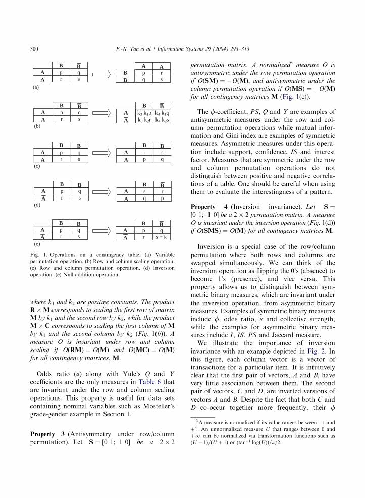
ARTICLE IN PRESS

B B A p q A r s

A A B p r B q s

B B A p q A r s

B B A k3 k1p k4 k1q A k3 k2r k4 k2s

B B A p q A r s

B B A r s A p q

B B A p q A r s

B B A s r A q p

B B A p q A r s

B B A p q A r s + k

(a)

(b)

(c)

(d)

(e)

Fig. 1. Operations on a contingency table. (a) Variable

permutation operation. (b) Row and column scaling operation.

(c) Row and column permutation operation. (d) Inversion

operation. (e) Null addition operation.

3A measure is normalized if its value ranges between 1 and

þ1: An unnormalized measure U that ranges between 0 and

þN can be normalized via transformation functions such as

ðU 1Þ=ðU þ 1Þ or ðtan1 logðUÞÞ=p=2:


where k1 and k2 are positive constants. The product

R�M corresponds to scaling the first row of matrix

M by k1 and the second row by k2; while the product

M� C corresponds to scaling the first column of M

by k1 and the second column by k2 (Fig. 1(b)). A

measure O is invariant under row and column

scaling if OðRMÞ ¼ OðMÞ and OðMCÞ ¼ OðMÞfor all contingency matrices, M:

Odds ratio ðaÞ along with Yule’s Q and Y

coefficients are the only measures in Table 6 thatare invariant under the row and column scalingoperations. This property is useful for data setscontaining nominal variables such as Mosteller’sgrade-gender example in Section 1.

Property 3 (Antisymmetry under row/columnpermutation). Let S ¼ ½0 1; 1 0� be a 2 � 2

permutation matrix. A normalized3 measure O is

antisymmetric under the row permutation operation

if OðSMÞ ¼ OðMÞ; and antisymmetric under the

column permutation operation if OðMSÞ ¼ OðMÞfor all contingency matrices M (Fig. 1(c)).

The f-coefficient, PS; Q and Y are examples ofantisymmetric measures under the row and col-umn permutation operations while mutual infor-mation and Gini index are examples of symmetricmeasures. Asymmetric measures under this opera-tion include support, confidence, IS and interestfactor. Measures that are symmetric under the rowand column permutation operations do notdistinguish between positive and negative correla-tions of a table. One should be careful when usingthem to evaluate the interestingness of a pattern.

Property 4 (Inversion invariance). Let S ¼½0 1; 1 0� be a 2 � 2 permutation matrix. A measure

O is invariant under the inversion operation (Fig. 1(d))if OðSMSÞ ¼ OðMÞ for all contingency matrices M:

Inversion is a special case of the row/columnpermutation where both rows and columns areswapped simultaneously. We can think of theinversion operation as flipping the 0’s (absence) tobecome 1’s (presence), and vice versa. Thisproperty allows us to distinguish between sym-metric binary measures, which are invariant underthe inversion operation, from asymmetric binarymeasures. Examples of symmetric binary measuresinclude f; odds ratio, k and collective strength,while the examples for asymmetric binary mea-sures include I ; IS; PS and Jaccard measure.

We illustrate the importance of inversioninvariance with an example depicted in Fig. 2. Inthis figure, each column vector is a vector oftransactions for a particular item. It is intuitivelyclear that the first pair of vectors, A and B; havevery little association between them. The secondpair of vectors, C and D; are inverted versions ofvectors A and B: Despite the fact that both C andD co-occur together more frequently, their f

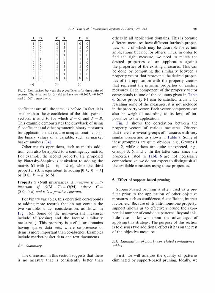
ARTICLE IN PRESS

1000000001

0000100000

0111111110

1111011111

A B C D

(a) (b)

0111111110

0000100000

(c)

E F

Fig. 2. Comparison between the f-coefficients for three pairs of

vectors. The f values for (a), (b) and (c) are 0:1667; 0:1667

and 0.1667, respectively.


coefficient are still the same as before. In fact, it issmaller than the f-coefficient of the third pair ofvectors, E and F ; for which E ¼ C and F ¼ B:This example demonstrates the drawback of usingf-coefficient and other symmetric binary measuresfor applications that require unequal treatments ofthe binary values of a variable, such as marketbasket analysis [34].

Other matrix operations, such as matrix addi-tion, can also be applied to a contingency matrix.For example, the second property, P2, proposedby Piatetsky-Shapiro is equivalent to adding thematrix M with ½k k; k k�; while the thirdproperty, P3; is equivalent to adding ½0 k; 0 k�or ½0 0; k k� to M:

Property 5 (Null invariance). A measure is null-

invariant if OðMþ CÞ ¼ OðMÞ where C ¼½0 0; 0 k� and k is a positive constant.

For binary variables, this operation correspondsto adding more records that do not contain thetwo variables under consideration, as shown inFig. 1(e). Some of the null-invariant measuresinclude IS (cosine) and the Jaccard similaritymeasure, z: This property is useful for domainshaving sparse data sets, where co-presence ofitems is more important than co-absence. Examplesinclude market-basket data and text documents.

4.3. Summary

The discussion in this section suggests that thereis no measure that is consistently better than

others in all application domains. This is becausedifferent measures have different intrinsic proper-ties, some of which may be desirable for certainapplications but not for others. Thus, in order tofind the right measure, we need to match thedesired properties of an application againstthe properties of the existing measures. This canbe done by computing the similarity between aproperty vector that represents the desired proper-ties of the application with the property vectorsthat represent the intrinsic properties of existingmeasures. Each component of the property vectorcorresponds to one of the columns given in Table6. Since property P1 can be satisfied trivially byrescaling some of the measures, it is not includedin the property vector. Each vector component canalso be weighted according to its level of im-portance to the application.

Fig. 3 shows the correlation between theproperty vectors of various measures. Observethat there are several groups of measures with verysimilar properties, as shown in Table 7. Some ofthese groupings are quite obvious, e.g., Groups 1and 2, while others are quite unexpected, e.g.,Groups 3, 6, and 7. In the latter case, since theproperties listed in Table 6 are not necessarilycomprehensive, we do not expect to distinguish allthe available measures using these properties.

5. Effect of support-based pruning

Support-based pruning is often used as a pre-filter prior to the application of other objectivemeasures such as confidence, f-coefficient, interestfactor, etc. Because of its anti-monotone property,support allows us to effectively prune the expo-nential number of candidate patterns. Beyond this,little else is known about the advantages ofapplying this strategy. The purpose of this sectionis to discuss two additional effects it has on the restof the objective measures.

5.1. Elimination of poorly correlated contingency

tables

First, we will analyze the quality of patternseliminated by support-based pruning. Ideally, we

ARTICLE IN PRESS

1 2 3 4 5 6 7 8 9 10 11 12 13 14 15 16 17 18 19 20 21

Correlation

Col Strength

PS

Mutual Info

CF

Kappa

Gini

Lambda

Odds ratio

Yule Y

Yule Q

J-measure

Laplace

Support

Confidence

Conviction

Interest

Klosgen

Added Value

Jaccard

IS -1

-0.8

-0.6

-0.4

-0.2

0

0.2

0.4

0.6

0.8

1

Fig. 3. Correlation between measures based on their property vector. Note that the column labels are the same as the row labels.

Table 7

Groups of objective measures with similar properties


prefer to eliminate only patterns that are poorlycorrelated. Otherwise, we may end up missing toomany interesting patterns.

To study this effect, we have created a syntheticdata set that contains 100; 000 2 � 2 contingencytables. Each table contains randomly populated fij

values subjected to the constraintP

i;j fij ¼ 1: Thesupport and f-coefficient for each table can becomputed using the formula shown in Table 5. Byexamining the distribution of f-coefficient values,we can determine whether there are any highlycorrelated patterns inadvertently removed as aresult of support-based pruning.

For this analysis, we apply two kinds ofsupport-based pruning strategies. The first strategyis to impose a minimum support threshold on the

value of f11: This approach is identical to thesupport-based pruning strategy employed by mostof the association analysis algorithms. The secondstrategy is to impose a maximum support thresh-old on both f1þ and fþ1: This strategy is equivalentto removing the most frequent items from a dataset (e.g., staple products such as sugar, bread, andmilk). The results for both of these experiments areillustrated in Figs. 4(a) and (b).

For the entire data set of 100,000 tables, the f-coefficients are normally distributed around f ¼ 0;as depicted in the upper left-hand corner of bothgraphs. When a maximum support threshold isimposed, the f-coefficient of the eliminated tablesfollows a bell-shaped distribution, as shown inFig. 4(a). In other words, imposing a maximumsupport threshold tends to eliminate uncorrelated,positively correlated, and negatively correlatedtables at equal proportions. This observation canbe explained by the nature of the synthetic data—since the frequency counts of the contingencytables are generated randomly, the eliminatedtables also have a very similar distribution as thef-coefficient distribution for the entire data.

On the other hand, if a lower bound of supportis specified (Fig. 4(b)), most of the contingencytables removed are either uncorrelated ðf ¼ 0Þ ornegatively correlated ðfo0Þ: This observation is

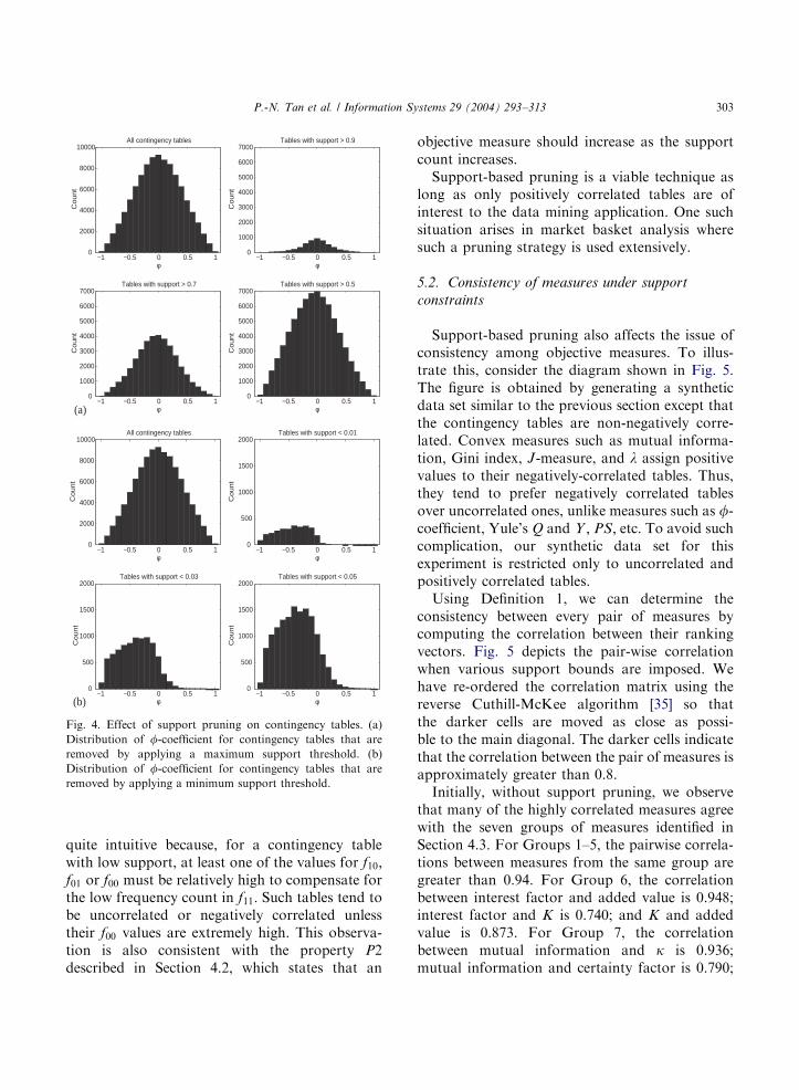
ARTICLE IN PRESS

−1 −0.5 0 0.5 10

2000

4000

6000

8000

10000All contingency tables

Co

un

t

φ−1 −0.5 0 0.5 1

0

1000

2000

3000

4000

5000

6000

7000Tables with support > 0.9

Co

un

t

φ

−1 −0.5 0 0.5 10

1000

2000

3000

4000

5000

6000


Co

unt

φ−1 −0.5 0 0.5 1

0

1000

2000

3000

4000

5000

6000


Co

unt

φ

−1 −0.5 0 0.5 10

2000

4000

6000

8000

10000All contingency tables

Co

un

t

φ−1 −0.5 0 0.5 1

0

500

1000

1500

2000Tables with support < 0.01

Co

un

t

φ

−1 −0.5 0 0.5 10

500

1000

1500


Co

un

t

φ−1 −0.5 0 0.5 1

0

500

1000

1500


Co

un

t

φ

(a)

(b)

Fig. 4. Effect of support pruning on contingency tables. (a)

Distribution of f-coefficient for contingency tables that are

removed by applying a maximum support threshold. (b)

Distribution of f-coefficient for contingency tables that are

removed by applying a minimum support threshold.


quite intuitive because, for a contingency tablewith low support, at least one of the values for f10;f01 or f00 must be relatively high to compensate forthe low frequency count in f11: Such tables tend tobe uncorrelated or negatively correlated unlesstheir f00 values are extremely high. This observa-tion is also consistent with the property P2described in Section 4.2, which states that an

objective measure should increase as the supportcount increases.

Support-based pruning is a viable technique aslong as only positively correlated tables are ofinterest to the data mining application. One suchsituation arises in market basket analysis wheresuch a pruning strategy is used extensively.

5.2. Consistency of measures under support

constraints

Support-based pruning also affects the issue ofconsistency among objective measures. To illus-trate this, consider the diagram shown in Fig. 5.The figure is obtained by generating a syntheticdata set similar to the previous section except thatthe contingency tables are non-negatively corre-lated. Convex measures such as mutual informa-tion, Gini index, J-measure, and l assign positivevalues to their negatively-correlated tables. Thus,they tend to prefer negatively correlated tablesover uncorrelated ones, unlike measures such as f-coefficient, Yule’s Q and Y ; PS; etc. To avoid suchcomplication, our synthetic data set for thisexperiment is restricted only to uncorrelated andpositively correlated tables.

Using Definition 1, we can determine theconsistency between every pair of measures bycomputing the correlation between their rankingvectors. Fig. 5 depicts the pair-wise correlationwhen various support bounds are imposed. Wehave re-ordered the correlation matrix using thereverse Cuthill-McKee algorithm [35] so thatthe darker cells are moved as close as possi-ble to the main diagonal. The darker cells indicatethat the correlation between the pair of measures isapproximately greater than 0.8.

Initially, without support pruning, we observethat many of the highly correlated measures agreewith the seven groups of measures identified inSection 4.3. For Groups 1–5, the pairwise correla-tions between measures from the same group aregreater than 0.94. For Group 6, the correlationbetween interest factor and added value is 0.948;interest factor and K is 0.740; and K and addedvalue is 0.873. For Group 7, the correlationbetween mutual information and k is 0.936;mutual information and certainty factor is 0.790;

ARTICLE IN PRESS

All Pairs

1 2 3 4 5 6 7 8 9 10 11 12 13 14 15 16 17 18 19 20 21

CF Conviction

Yule Y Odds ratio Yule Q

Mutual Info Correlation Kappa

Col StrengthGini

J measure PS

Klosgen Interest

Added Value Confidence

Laplace Jaccard

IS Lambda Support 0

0.2

0.4

0.6

0.8

10.000 <= support <= 0.5

1 2 3 4 5 6 7 8 9 10 11 12 13 14 15 16 17 18 19 20 21

CF Conviction



Col StrengthGini

J measure PS

Klosgen Interest


Laplace Jaccard

IS Lambda Support 0

0.2

0.4

0.6

0.8

1

0.050 <= support <= 1.0

1 2 3 4 5 6 7 8 9 10 11 12 13 14 15 16 17 18 19 20 21

CF Conviction



Col StrengthGini

J measure PS

Klosgen Interest


Laplace Jaccard

IS Lambda Support 0

0.2

0.4

0.6

0.8

10.050 <= support <= 0.5

1 2 3 4 5 6 7 8 9 10 11 12 13 14 15 16 17 18 19 20 21

CF Conviction



Col StrengthGini

J measure PS

Klosgen Interest


Laplace Jaccard

IS Lambda Support 0

0.2

0.4

0.6

0.8

1

Fig. 5. Similarity between measures at various ranges of support values. Note that the column labels are the same as the row labels.

Table 8

Effect of high-support items on interest factor


and k and certainty factor is 0.747. These resultssuggest that the properties defined in Table 6 mayexplain most of the high correlations in the upperleft-hand diagram shown in Fig. 5.

Next, we examine the effect of applying amaximum support threshold to the contingencytables. The result is shown in the upper right-handdiagram. Notice the growing region of dark cellscompared to the previous case, indicating thatmore measures are becoming highly correlatedwith each other. Without support-based pruning,nearly 40% of the pairs have correlation above0.85. With maximum support pruning, this per-centage increases to more than 68%. For example,interest factor, which is quite inconsistent withalmost all other measures except for added value,have become more consistent when high-supportitems are removed. This observation can beexplained as an artifact of interest factor. Considerthe contingency tables shown in Table 8, where A

and B correspond to a pair of uncorrelated items,

while C and D correspond to a pair of perfectlycorrelated items. However, because the support foritem C is very high, IðC;DÞ ¼ 1:0112; which isclose to the value for statistical independence. Byeliminating the high support items, we may resolvethis type of inconsistency between interest factorand other objective measures.

Our result also suggests that imposing a mini-mum support threshold does not seem to improvethe consistency among measures. However, when

ARTICLE IN PRESS


it is used along with a maximum support thresh-old, the correlations among measures do showsome slight improvements compared to applyingthe maximum support threshold alone—morethan 71% of the pairs have correlation above0.85. This analysis suggests that imposing a tighterbound on the support of association patterns mayforce many measures become highly correlatedwith each other.

6. Table standardization

Standardization is a widely used technique instatistics, political science, and social sciencestudies to handle contingency tables that havedifferent marginals. Mosteller suggested thatstandardization is needed to get a better idea ofthe underlying association between variables [3],by transforming an existing table so that theirmarginals become equal, i.e., f �1þ ¼ f �0þ ¼ f �þ1 ¼f �þ0 ¼ N=2 (see Table 9). A standardized table isuseful because it provides a visual depiction ofhow the joint distribution of two variables wouldlook like after eliminating biases due to non-uniform marginals.

6.1. Effect of non-uniform marginals

Standardization is important because somemeasures can be affected by differences in themarginal totals. To illustrate this point, consider apair of contingency tables, X ¼ ½a b; c d� andY ¼ ½p q; r s�: We can compute the differencebetween the f-coefficients for both tables asfollows.

logðfX Þ ¼ logðad bcÞ 12½logða þ bÞ þ logða þ cÞ

þ logðb þ cÞ þ logðb þ dÞ�; ð1Þ

Table 9

Table standardization

logðfY Þ ¼ logðpq rsÞ 12½logðp þ qÞ þ logðp þ rÞ

þ logðq þ sÞ þ logðr þ sÞ�; ð2Þ

where the f-coefficient is expressed as a logarith-mic value to simplify the calculations. Thedifference between the two coefficients can bewritten as

logðfX Þ logðfY Þ ¼ D1 0:5D2;

where

D1 ¼ logðad bcÞ logðpq rsÞ

and

D2 ¼ logða þ bÞða þ cÞðb þ cÞðb þ dÞ

logðp þ qÞðp þ rÞðq þ sÞðr þ sÞ:

If the marginal totals for both tables are identical,then any observed difference between logðfX Þ andlogðfY Þ comes from the first term, D1: Conversely,if the marginals are not identical, then theobserved difference in f can be caused by eitherD1; D2; or both.

The problem of non-uniform marginals issomewhat analogous to using accuracy for evalu-ating the performance of classification models. If adata set contains 99% examples of class 0 and 1%examples of class 1, then a classifier that producesmodels that classify every test example to be class 0would have a high accuracy, despite performingmiserably on class 1 examples. Thus, accuracy isnot a reliable measure because it can be easilyobscured by differences in the class distribution.One way to overcome this problem is by stratifyingthe data set so that both classes have equalrepresentation during model building. A similar‘‘stratification’’ strategy can be used to handlecontingency tables with non-uniform support,i.e., by standardizing the frequency counts of acontingency table.

ARTICLE IN PRESS


6.2. IPF standardization

Mosteller presented the following iterativestandardization procedure, which is called theIterative Proportional Fitting algorithm or IPF[4], for adjusting the cell frequencies of a tableuntil the desired margins, f �iþ and f �þj ; are obtained:

Row scaling:

fðkÞ

ij ¼ fðk1Þ

ij �f �iþ

fðk1Þ

iþ

; ð3Þ

Column scaling:

fðkþ1Þ

ij ¼ fðkÞ

ij �f �þj

fðkÞþj

: ð4Þ

An example of the IPF standardization procedureis demonstrated in Fig. 6.

Theorem 1. The IPF standardization procedure is

equivalent to multiplying the contingency matrix

M ¼ ½a b; c d� with

k1 0

0 k2

" #a b

c d

" #k3 0

0 k4

" #;

where k1; k2; k3 and k4 are products of the row and

column scaling factors.

Proof. The following lemma is needed to provethe above theorem.

15 10 2535 40 7550 50 100

30.00 20.00 50.0023.33 26.67 50.0053.33 46.67 100.00

28.12 21.43 49.5521.88 28.57 50.4550.00 50.00 100.00

28.38 21.62 50.0021.68 28.32 50.0050.06 49.94 100.00

Original Table

StandardizedTable

k=0 k=1

k=3 k=2

28.35 21.65 50.0021.65 28.35 50.0050.00 50.00 100.00

28.34 21.65 49.9921.66 28.35 50.0150.00 50.00 100.00

k=4 k=5

Fig. 6. Example of IPF standardization.

Lemma 1. The product of two diagonal matrices is

also a diagonal matrix.

This lemma can be proved in the following way.Let M1 ¼ ½f1 0; 0 f2� and M2 ¼ ½f3 0; 0 f4�: Then,M1 � M2 ¼ ½ðf1f3Þ 0; 0 ðf2f4Þ�; which is also adiagonal matrix.

To prove Theorem 1, we also need to useDefinition 2, which states that scaling the row andcolumn elements of a contingency table is equiva-lent to multiplying the contingency matrix by ascaling matrix ½k1 0; 0 k2�: For IPF, during thekth iteration, the rows are scaled by f �iþ=f

ðk1Þiþ ;

which is equivalent to multiplying the matrix by½f �1þ=f

ðk1Þ1þ 0; 0 f �0þ=f

ðk1Þ0þ � on the left. Meanwhile,

during the ðk þ 1Þth iteration, the columns arescaled by f �þj=f

ðkÞþj ; which is equivalent to multi-

plying the matrix by ½f �þ1=fðkÞþ1 0; 0 f �þ0=f

ðkÞþ0 � on the

right. Using Lemma 1, we can show that the resultof multiplying the row and column scalingmatrices is equivalent to

f �1þ=fðmÞ1þ ?f �1þ=f

ð0Þ1þ 0

0 f �0þ=fðmÞ0þ ?f �0þ=f

ð0Þ0þ

" #

�a b

c d

" #

�f �þ1=f

ðmþ1Þþ1 ?f �þ1=f

ð1Þþ1 0

0 f �þ0=fðmþ1Þþ0 ?f �þ0=f

ð1Þþ0

" #

thus, proving Theorem 1.

The above theorem also suggests that theiterative steps of IPF can be replaced by a singlematrix multiplication operation if the scalingfactors k1; k2; k3 and k4 are known. In Section 6,we will provide a non-iterative solution for k1; k2;k3 and k4:

6.3. Consistency of measures under table

standardization

Interestingly, the consequence of doing standar-dization goes beyond ensuring uniform margins ina contingency table. More importantly, if we applydifferent measures from Table 5 on the standar-dized, positively correlated tables, their rankings

ARTICLE IN PRESS


become identical. To the best of our knowledge,this fact has not been observed by anyone elsebefore. As an illustration, Table 10 shows theresults of ranking the standardized contingencytables for each example given in Table 3. Observethat the rankings are identical for all the measures.This observation can be explained in the followingway. After standardization, the contingency ma-trix has the following form ½x y; y x�; where x ¼f �11 and y ¼ N=2 x: The rankings are the samebecause many measures of association (specifi-cally, all 21 considered in this paper) are mono-tonically increasing functions of x when applied tothe standardized, positively correlated tables. Weillustrate this with the following example.

Example 1. The f-coefficient of a standardizedtable is

f ¼x2 ðN=2 xÞ2

ðN=2Þ2¼

4x

N 1: ð5Þ

For a fixed N ; f is a monotonically increasingfunction of x: Similarly, we can show that othermeasures such as a; I ; IS; PS; etc., are alsomonotonically increasing functions of x:

The only exceptions to this are l; Gini index,mutual information, J-measure, and Klosgen’s K ;which are convex functions of x: Nevertheless,these measures are monotonically increasing whenwe consider only the values of x between N=4 andN=2; which correspond to non-negatively corre-lated tables. Since the examples given in Table 3are positively correlated, all 21 measures given in

Table 10

Rankings of contingency tables after IPF st

this paper produce identical ordering for theirstandardized tables.

6.4. Generalized standardization procedure

Since each iterative step in IPF corresponds toeither a row or column scaling operation, oddsratio is preserved throughout the transformation(Table 6). In other words, the final rankings on thestandardized tables for any measure are consistentwith the rankings produced by odds ratio on theoriginal tables. For this reason, a casual observermay think that odds ratio is perhaps the bestmeasure to use. This is not true because there areother ways to standardize a contingency table. Toillustrate other standardization schemes, we firstshow how to obtain the exact solutions for f �ij susing a direct approach. If we fix the standardizedtable to have equal margins, this forces the f �ij s tosatisfy the following equations:

f �11 ¼ f �00; f �10 ¼ f �01; f �11 þ f �10 ¼ N=2: ð6Þ

Since there are only three equations in (6), wehave the freedom of choosing a fourth equationthat will provide a unique solution to the tablestandardization problem. In Mosteller’s approach,the fourth equation is used to ensure that the oddsratio of the original table is the same as the oddsratio of the standardized table. This leads to thefollowing conservation equation:

f11 f00

f10 f01¼

f �11 f �00

f �10 f �01

: ð7Þ

andardization

ARTICLE IN PRESS

4Note that although the standardized table preserves the

invariant measure, these intermediate steps of row or column

scaling and addition of null values may not preserve the

measure.


After combining Eqs. (6) and (7), the followingsolutions are obtained:

f �11 ¼ f �00 ¼N

ffiffiffiffiffiffiffiffiffiffiffiffif11 f00

p2ð


pþ


pÞ; ð8Þ

f �10 ¼ f �01 ¼N


p2ð


pþ


pÞ: ð9Þ

The above analysis suggests the possibility of usingother standardization schemes for preservingmeasures besides the odds ratio. For example,the fourth equation could be chosen to preservethe invariance of IS (cosine measure). This wouldlead to the following conservation equation:

f11ffiffiffiffiffiffiffiffiffiffiffiffiffiffiffiffiffiffiffiffiffiffiffiffiffiffiffiffiffiffiffiffiffiffiffiffiffiffiffiðf11 þ f10Þðf11 þ f01Þ

p ¼f �11ffiffiffiffiffiffiffiffiffiffiffiffiffiffiffiffiffiffiffiffiffiffiffiffiffiffiffiffiffiffiffiffiffiffiffiffiffiffiffi

ðf �11 þ f �10Þðf�11 þ f �01Þ

p ;

ð10Þ

whose solutions are:

f �11 ¼ f �00 ¼Nf11

2ffiffiffiffiffiffiffiffiffiffiffiffiffiffiffiffiffiffiffiffiffiffiffiffiffiffiffiffiffiffiffiffiffiffiffiffiffiffiffiðf11 þ f10Þðf11 þ f01Þ

p ; ð11Þ

f �10 ¼ f �01 ¼N

2

ffiffiffiffiffiffiffiffiffiffiffiffiffiffiffiffiffiffiffiffiffiffiffiffiffiffiffiffiffiffiffiffiffiffiffiffiffiffiffiðf11 þ f10Þðf11 þ f01Þ

p f11ffiffiffiffiffiffiffiffiffiffiffiffiffiffiffiffiffiffiffiffiffiffiffiffiffiffiffiffiffiffiffiffiffiffiffiffiffiffiffi

ðf11 þ f10Þðf11 þ f01Þp : ð12Þ

Thus, each standardization scheme is closelytied to a specific invariant measure. If IPFstandardization is natural for a given application,then odds ratio is the right measure to use. Inother applications, a standardization schemethat preserves some other measure may be moreappropriate.

6.5. General solution of standardization procedure

In Theorem 1, we showed that the IPFprocedure can be formulated in terms of a matrixmultiplication operation. Furthermore, the leftand right multiplication matrices are equivalentto scaling the row and column elements of theoriginal matrix by some constant factors k1; k2; k3

and k4: Note that one of these factors is actuallyredundant; theorem 1 can be stated in terms ofthree parameters, k0

1; k02 and k0

3; i.e.,

k1 0

0 k2

" #a b

c d

" #k3 0

0 k4

" #

¼k0

1 0

0 k02

" #a b

c d

" #k0

3 0

0 1

" #:

Suppose M ¼ ½a b; c d� is the original contin-gency table and Ms ¼ ½x y; y x� is the standar-dized table. We can show that any generalizedstandardization procedure can be expressed interms of three basic operations: row scaling,column scaling, and addition of null values.4

k1 0

0 k2

" #a b

c d

" #k3 0

0 1

" #þ

0 0

0 k4

" #

¼x y

y x

" #:

This matrix equation can be easily solved toobtain

k1 ¼y

b; k2 ¼

y2a

xbc; k3 ¼

xb

ay;

k4 ¼ x 1 ad=bc

x2=y2

� �:

For IPF, since ad=bc ¼ x2=y2; therefore k4 ¼ 0;and the entire standardization procedure can beexpressed in terms of row and column scalingoperations.

7. Measure selection based on rankings by experts

Although the preceding sections describe twoscenarios in which many of the measures becomeconsistent with each other, such scenarios may nothold for all application domains. For example,support-based pruning may not be useful fordomains containing nominal variables, while inother cases, one may not know the exact standar-dization scheme to follow. For such applications,an alternative approach is needed to find the bestmeasure.

ARTICLE IN PRESS


In this section, we describe a subjective ap-proach for finding the right measure based on therelative rankings provided by domain experts.Ideally, we want the experts to rank all thecontingency tables derived from the data. Theserankings can help us identify the measure thatis most consistent with the expectation of theexperts. For example, we can compare thecorrelation between the rankings produced bythe existing measures against the rankings pro-vided by the experts and select the measure thatproduces the highest correlation.

Unfortunately, asking the experts to rank all thetables manually is often impractical. A morepractical approach is to provide a smaller set ofcontingency tables to the experts for ranking anduse this information to determine the mostappropriate measure. To do this, we have toidentify a small subset of contingency tables thatoptimizes the following criteria:

1.
The subset must be small enough to allowdomain experts to rank them manually. On theother hand, the subset must be large enough toensure that choosing the best measure from thesubset is almost equivalent to choosing the bestmeasure when the rankings for all contingencytables are available.
2.
The subset must be diverse enough to captureas much conflict of rankings as possible amongthe different measures.
The first criterion is usually determined by theexperts because they are the ones who can decidethe number of tables they are willing to rank.Therefore, the only criterion we can optimizealgorithmically is the diversity of the subset. In thispaper, we investigate two subset selection algo-rithms: RANDOM algorithm and DISJOINTalgorithm.

RANDOM Algorithm. This algorithm ran-domly selects k of the N tables to be presentedto the experts. We expect the RANDOM algo-rithm to work poorly when k5N : Nevertheless,the results obtained using this algorithm is stillinteresting because they can serve as a baselinereference.

DISJOINT Algorithm. This algorithm attemptsto capture the diversity of the selected subset interms of

1.
Conflicts in the rankings produced bythe existing measures. A contingency tablewhose rankings are ð1; 2; 3; 4; 5Þ accordingto five different measures have larger rankingconflicts compared to another table whoserankings are ð3; 2; 3; 2; 3Þ: One way tocapture the ranking conflicts is by computingthe standard deviation of the ranking vector.
2.
Range of rankings produced by the existingmeasures. Suppose there are five contin-gency tables whose rankings are given asfollows.
Table t1:
1 2 1 2 1 Table t2: 10 11 10 11 10 Table t3: 2000 2001 2000 2001 2000 Table t4: 3090 3091 3090 3091 3090 Table t5: 4000 4001 4000 4001 4000
The standard deviation of the rankings areidentical for all the tables. If we are forcedto choose three of the five tables, it is better toselect t1; t3; and t5 because they span a widerange of rankings. In other words, these tablesare ‘‘furthest’’ apart in terms of their averagerankings.

A high-level description of the algorithm is pre-sented in Table 11. First, the algorithm computesthe average and standard deviation of rankings forall the tables (step 2). It then adds the contingencytable that has the largest amount of rankingconflicts into the result set Z (step 3). Next, thealgorithm computes the ‘‘distance’’ between eachpair of table in step 4. It then greedily tries tofind k tables that are ‘‘furthest’’ apart accordingto their average rankings and produce thelargest amount of ranking conflicts in termsof the standard deviation of their ranking vector(step 5a).

The DISJOINT algorithm can be quite expen-sive to implement because we need to compute thedistance between all ðN � ðN 1ÞÞ=2 pairs oftables. To avoid this problem, we introduce anoversampling parameter, p; where 1op5JN=kn;so that instead of sampling from the entire N

ARTICLE IN PRESS

Table 11

The DISJOINT algorithm

a b

c dA = 0

B = 1 B = 0

A = 1

.

.

.

All Contingency Tables

select ktables

M1 M2 … MpM1M2…Mp

Compute similaritybetween different

measures

Compute similaritybetween different

measures

Goal: Minimize thedifference

a b

c dA = 0

B = 1 B = 0

A = 1

a b

c dA = 0

B = 1 B = 0

A = 1

M1 M2 … MpT1T2…TN

M1 M2 … MpM1M2…Mp

M1 M2 … MpT1'T2'…Tk'

Rank tables accordingto various measures

Rank tables accordingto various measures

T1

T2

TN

S ST s

.

.

.

Subset of ContingencyTables

a b

c dA = 0

B = 1 B = 0

A = 1

T1'

Tk'

a b

c dA = 0

B = 1 B = 0

A = 1 PresentedTo

DomainExperts

Fig. 7. Evaluating the contingency tables selected by a subset

selection algorithm.

Table 12

Data sets used in our experiments

5Only frequent items are considered, i.e., those with support

greater than a user-specified minimum support threshold.


tables, we select the k tables from a sub-populationthat contains only k � p tables. This reducesthe complexity of the algorithm significantly toðkp � ðkp 1ÞÞ=2 distance computations.

7.1. Experimental methodology

To evaluate the effectiveness of the subsetselection algorithms, we use the approach shownin Fig. 7. Let T be the set of all contingency tablesand S be the tables selected by a subset selectionalgorithm. Initially, we rank each contingencytable according to all the available measures. Thesimilarity between each pair of measure is thencomputed using Pearson’s correlation coefficient.If the number of available measures is p; then ap � p similarity matrix will be created for each set,T and S: A good subset selection algorithm shouldminimize the difference between the similaritymatrix computed from the subset, Ss; and thesimilarity matrix computed from the entire set ofcontingency tables, ST : The following distancefunction is used to determine the differencebetween the two similarity matrices:

DðSs;ST Þ ¼ maxi;j

jST ði; jÞ Ssði; jÞj: ð13Þ

If the distance is small, then we consider S as agood representative of the entire set of contingencytables T :

7.2. Experimental evaluation

We have conducted our experiments using thedata sets shown in Table 12. For each data set, werandomly sample 100,000 pairs of binary items5 as

ARTICLE IN PRESS

0 10 20 30 40 50 60 70 80 90 1000

0.1

0.2

0.3

0.4

0.5

0.6

0.7

0.8

0.9

Sample size, k

Ave

rage

Dis

tanc

e, D

RANDOMDISJOINT (p=10)DISJOINT (p=20)

Fig. 8. Average distance between similarity matrix computed

from the subset (Ss) and the similarity matrix computed from

the entire set of contingency tables (ST ) for the re0 data set.

re0 Q Y κκκκ PS F AV K I c L IS ξξξξ s S λ λ λ λ M J G αααα V

All tables 8 7 4 16 15 10 11 9 17 18 2 12 19 3 20 5 1 13 6 14

k=20 6 6 5 16 13 10 11 12 17 18 2 15 19 4 20 3 1 9 6 14

la1 Q Y κκκκ PS F AV K I c L IS ξξξξ s S λ λ λ λ M J G αααα V

All tables 10 9 2 7 5 3 6 16 18 17 13 14 19 1 20 12 11 15 8 4

k=20 13 13 2 5 8 3 6 16 18 17 10 11 19 1 20 9 4 12 13 7

Product Q Y κκκκ PS F AV K I c L IS ξξξξ s S λ λ λ λ M J G αααα V

All tables 12 11 3 10 8 7 14 16 17 18 1 4 19 2 20 5 6 15 13 9

k=20 13 13 2 7 11 10 9 17 16 18 1 4 19 3 20 6 5 8 13 11

S&P500 Q Y κκκκ PS F AV K I c L IS ξξξξ s S λ λ λ λ M J G αααα V

All tables 9 8 1 10 6 3 4 11 15 14 12 13 19 2 20 16 18 17 7 5

k=20 7 7 2 10 4 3 6 11 17 18 12 13 19 1 20 15 14 16 7 4

E-Com Q Y κκκκ PS F AV K I c L IS ξξξξ s S λ λ λ λ M J G αααα V

All tables 9 8 3 7 14 13 16 11 17 18 1 4 19 2 20 6 5 12 10 15

k=20 7 7 3 10 15 14 13 11 17 18 1 4 19 2 20 6 5 12 7 15

Census Q Y κκκκ PS F AV K I c L IS ξξξξ s S λ λ λ λ M J G αααα V

All tables 10 10 2 3 7 5 4 11 13 12 14 15 16 1 20 19 18 17 10 6

k=20 6 6 3 2 9 5 4 11 13 12 14 15 16 1 17 18 19 20 6 9

All tables: Rankings when all contingency tables are ordered.

k=20 : Rankings when 20 of the selected tables are ordered.Fig. 9. Ordering of measures based on contingency tables selected by the DISJOINT algorithm.


our initial set of contingency tables. We then applythe RANDOM and DISJOINT table selectionalgorithms on each data set and compare thedistance function D at various sample sizes k: Foreach value of k; we repeat the procedure 20 timesand compute the average distance D: Fig. 8 showsthe relationships between the average distance D

and sample size k for the re0 data set. As expected,our results indicate that the distance function D

decreases with increasing sample size, mainlybecause the larger the sample size, the moresimilar it is to the entire data set. Furthermore,the DISJOINT algorithm does a substantiallybetter job than random sampling in terms ofchoosing the right tables to be presented to thedomain experts. This is because it tends to select

ARTICLE IN PRESS


tables that are furthest apart in terms of theirrelative rankings and tables that create a hugeamount of ranking conflicts. Even at k ¼ 20; thereis little difference (Do0:15) between the similaritymatrices Ss and ST :

We complement our evaluation above by show-ing that the ordering of measures produced by theDISJOINT algorithm on even a small sample of20 tables is quite consistent with the ordering ofmeasures if the entire tables are ranked by thedomain experts. To do this, we assume that therankings provided by the experts is identical tothe rankings produced by one of the measures, say,the f-coefficient. Next, we remove f from the setof measures M considered by the DISJOINTalgorithm and repeat the experiments above withk ¼ 20 and p ¼ 10: We compare the best measureselected by our algorithm against the best measureselected when the entire set of contingency tables isavailable. The results are depicted in Fig. 9. Innearly all cases, the difference in the ranking of ameasure between the two (all tables versus asample of 20 tables) is 0 or 1.

8. Conclusions

This paper presents several key properties foranalyzing and comparing the various objectivemeasures developed in the statistics, social science,machine learning, and data mining literature. Dueto differences in some of their properties, asignificant number of these measures may provideconflicting information about the interestingnessof a pattern. However, we show that there are twosituations in which the measures may becomeconsistent with each other, namely, when support-based pruning or table standardization are used.We also show another advantage of using supportin terms of eliminating uncorrelated and poorlycorrelated patterns. Finally, we develop an algo-rithm for selecting a small set of tables such that anexpert can find a suitable measure by looking atjust this small set of tables.

For future work, we plan to extend the analysisbeyond two-way relationships. Only a handful ofthe measures shown in Table 5 (such as support,interest factor, and PS measure) can be general-ized to multi-way relationships. Analyzing such

relationships is much more cumbersome becausethe number of cells in a contingency table growsexponentially with k: New properties may also beneeded to capture the utility of an objectivemeasure in terms of analyzing k-way contingencytables. This is because a good objective measuremust be able to distinguish between the directassociation among k variables from their partialassociations. More research is also needed toderive additional properties that can distinguishbetween some of the similar measures shown inTable 7. In addition, new properties or measuresmay be needed to analyze the relationship betweenvariables of different types. A common approachfor doing this is to transform one of the variablesinto the same type as the other. For example, givena pair of variables, consisting of one continuousand one categorical variable, we can discretize thecontinuous variable and map each interval into adiscrete variable before applying an objectivemeasure. In doing so, we may lose informationabout the relative ordering among the discretizedintervals.

References

[1] R. Agrawal, T. Imielinski, A. Swami, Mining association

rules between sets of items in large databases, in:

Proceedings of 1993 ACM-SIGMOD International Con-

ference on Management of Data, Washington, DC, May

1993, pp. 207–216.

[2] R. Agrawal, T. Imielinski, A. Swami, Database mining: a

performance perspective, IEEE Trans. Knowledge Data

Eng. 5 (6) (1993) 914–925.

[3] F. Mosteller, Association and estimation in contingency

tables, J. Am. Stat. Assoc. 63 (1968) 1–28.

[4] A. Agresti, Categorical Data Analysis, Wiley, New York,

1990.

[5] G. Piatetsky-Shapiro, Discovery, analysis and presentation

of strong rules, in: G. Piatetsky-Shapiro, W. Frawley

(Eds.), Knowledge Discovery in Databases, MIT Press,

Cambridge, MA, 1991, pp. 229–248.

[6] R.J. Hilderman, H.J. Hamilton, B. Barber, Ranking the

interestingness of summaries from data mining systems, in:

Proceedings of the 12th International Florida Artificial

Intelligence Research Symposium (FLAIRS’99), Orlando,

FL, May 1999, pp. 100–106.

[7] R.J. Hilderman, H.J. Hamilton, Knowledge Discovery and

Measures of Interest, Kluwer Academic Publishers,

Norwell, MA, 2001.

[8] I. Kononenko, On biases in estimating multi-valued

attributes, in: Proceedings of the Fourteenth International

ARTICLE IN PRESS


Joint Conference on Artificial Intelligence (IJCAI’95),

Montreal, Canada, 1995, pp. 1034–1040.

[9] R. Bayardo, R. Agrawal, Mining the most interesting

rules, in: Proceedings of the Fifth International Conference

on Knowledge Discovery and Data Mining, San Diego,

CA, August 1999, pp. 145–154.

[10] M. Gavrilov, D. Anguelov, P. Indyk, R. Motwani, Mining

the stock market: which measure is best? in: Proceedings of

the Sixth International Conference on Knowledge Dis-

covery and Data Mining, Boston, MA, 2000.

[11] Y. Zhao, G. Karypis, Criterion functions for document

clustering: experiments and analysis. Technical Report

TR01-40, Department of Computer Science, University of

Minnesota, 2001.

[12] L.A. Goodman, W.H. Kruskal, Measures of association

for cross-classifications, J. Am. Stat. Assoc. 49 (1968)

732–764.

[13] G.U. Yule, On the association of attributes in statistics,

Philos. Trans. R. Soc. A 194 (1900) 257–319.

[14] G.U. Yule, On the methods of measuring association

between two attributes, J. R. Stat. Soc. 75 (1912) 579–642.

[15] J. Cohen, A coefficient of agreement for nominal scales,

Educ. Psychol. Meas. 20 (1960) 37–46.

[16] T. Cover, J. Thomas, Elements of Information Theory,

New York, Wiley, 1991.

[17] P. Smyth, R.M. Goodman, Rule induction using informa-

tion theory, in: Gregory Piatetsky-Shapiro, William

Frawley (Eds.), Knowledge Discovery in Databases, MIT

Press, Cambridge, MA, 1991, pp. 159–176.

[18] L. Breiman, J. Friedman, R. Olshen, C. Stone, Classifica-

tion and Regression Trees, Chapman & Hall, New York,

1984.

[19] R. Agrawal, R. Srikant, Fast algorithms for mining

association rules in large databases, in: Proceedings of

the 20th VLDB Conference, Santiago, Chile, September

1994, pp. 487–499.

[20] P. Clark, R. Boswell, Rule induction with cn2: some recent

improvements, in: Proceedings of the European Working

Session on Learning EWSL-91, Porto, Portugal, 1991, pp.

151–163.

[21] S. Brin, R. Motwani, J. Ullman, S. Tsur, Dynamic itemset

counting and implication rules for market basket data, in:

Proceedings of 1997 ACM-SIGMOD International Con-

ference on Management of Data, Montreal, Canada, June

1997, pp. 255–264.

[22] S. Brin, R. Motwani, C. Silverstein, Beyond market

baskets: generalizing association rules to correlations,

in: Proceedings of 1997 ACM-SIGMOD International

Conference on Management of Data, Tucson, Arizona,

June 1997, pp. 255–264.

[23] C. Silverstein, S. Brin, R. Motwani, Beyond market

baskets: generalizing association rules to dependence

rules, Data Mining Knowledge Discovery 2 (1) (1998)

39–68.

[24] T. Brijs, G. Swinnen, K. Vanhoof, G. Wets, Using

association rules for product assortment decisions: a case

study, in: Proceedings of the Fifth International Con-

ference on Knowledge Discovery and Data Mining, San

Diego, CA, August 1999, pp. 254–260.

[25] C. Clifton, R. Cooley, Topcat: data mining for topic

identification in a text corpus, in: Proceedings of the 3rd

European Conference of Principles and Practice of Knowl-

edge Discovery in Databases, Prague, Czech Republic,

September 1999, pp. 174–183.

[26] W. DuMouchel, D. Pregibon, Empirical bayes screening

for multi-item associations, in: Proceedings of the Seventh

International Conference on Knowledge Discovery and

Data Mining, 2001, pp. 67–76.

[27] E. Shortliffe, B. Buchanan, A model of inexact reasoning

in medicine, Math. Biosci. 23 (1975) 351–379.

[28] C.C. Aggarwal, P.S. Yu, A new framework for itemset

generation, in: Proceedings of the 17th Symposium on

Principles of Database Systems, Seattle, WA, June 1998,

pp. 18–24.

[29] S. Sahar, Y. Mansour, An empirical evaluation of

objective interestingness criteria, in: SPIE Conference on

Data Mining and Knowledge Discovery, Orlando, FL,

April 1999, pp. 63–74.

[30] P.N. Tan, V. Kumar, Interestingness measures for

association patterns: a perspective, in: KDD 2000 Work-

shop on Postprocessing in Machine Learning and Data

Mining, Boston, MA, August 2000.

[31] C.J. van Rijsbergen, Information Retrieval, 2nd Edition,

Butterworths, London, 1979.

[32] W. Klosgen, Problems for knowledge discovery in

databases and their treatment in the statistics interpreter

explora, Int. J. Intell. Systems 7 (7) (1992) 649–673.

[33] M. Kamber, R. Shinghal, Evaluating the interestingness of

characteristic rules, in: Proceedings of the Second Inter-

national Conference on Knowledge Discovery and Data

Mining, Portland, Oregon, 1996, pp. 263–266.

[34] D. Hand, H. Mannila, P. Smyth, Principles of Data

Mining, MIT Press, Cambridge, MA, 2001.

[35] A. George, W.H. Liu, Computer Solution of Large Sparse

Positive Definite Systems, Series in Computational Mathe-

matics, Prentice-Hall, Englewood Cliffs, NJ, 1981.

selecting the right objective measure for association …cse.msu.edu/~ptan/papers/is.pdf ·...

Documents