Division of .I:;ricultural Scicnces in'I\ExSIn' OF cL\LirGRYl,i

\$'orking Paper So. SO5

kETkIODS FOR SELECTING 'TIE OPTIbWL. D'iX,X?lIG HEDGE llIEN PRODUCTION IS STOCHASTIC

Larry S. Karp

California Agricultural E4qeriment Station Giannini Foundation of Agricuitural Economics

Februnly 1986

METHODS FOR SELECTING THE OIiEOPTI D W C HEDGE WHEN PRODUCTION IS STOCHASTIC

BY

Larry S. Karp

Abstract

A dynamic hedging problem with stochastic production is solved. The

optimal feedback rules recognize that future hedges will be chosen optimally

based on the most current information. The resulting distribution of revenue

is analyzed numerically. This analysis enables the hedger to select his

appropriate level of risk aversion.

Larry S . Karp is an assistant professor of agricultural and resource

economics, University of California, Berkeley.

?.ETHODS FOR SELECTING TEE OPfIW DLmlIC HEDGE h1EN PRODUCTION IS STOCHASTIC

Introduction

Futures and forward markets insulate producers from the risk inherent in out-

put and price uncertainty. The possibility of hedging influences the produc-

tion decision. There is considerable literature on the joint problems of

optimal hedging and production. McKinnon derived the hedge which minimizes

the variance of income. The pavers by Danthine; Feder, Just, and Schmitz; and

Holthausen consider the more general expected utility maximization problem

with hedging. In a series of papers, Anderson and Danthine (1981, 1983a,

1983b) derive theoretical results using a mean-variance criterion. Hil-dreth

considers more general utility functions and stochastic production. Batlin

concentrates on the case where the date of maturity of the futures contracts

and the time of harvest do not coincide (the "imperfect time hedge"). Ho;

Karp (1986); and Marcus and Modest consider dynamic hedging in continuous

time. The papers by Berck (1981); Nelson; Peck; and Rolfo present empirical

results.

With the exception of Anderson and Danthine (1983b), Ho; Marcus and

Modest; and Karp (1986), these papers view the hedging decision as static.

The static approach includes the situation where hedges can be made at differ-

ent points in time, but the current hedge is determined as if a conunitment

were being made concerning future hedges. In this case there is no recogni-

tion that future hedges will be conditioned on information which will become

available in the future. The dynamic strateg* on the other hand, does anti-

cipate that future hedges will be optimally chosen. The solution to the

dynamic problem consists of rules which determi.ne the hedge as a function of

the most current information.

There have been two approaches to characterizing the dynamic hedge.

Marcus and Modest consider the case of a public firm which is able to make its

total return free of all systematic risk. Using arbitrage relations, the op-

timal hedge is shown to be independent of firm-specific characteristics such

as risk aversion. These results are not applicable to the unincorporated

private firm. The second approach is to choose a specific utility function

and specific stochastic processes and solve the resulting optimal control

problem. Anderson and Danthine (1983b) use a mean-variance criterion in a

two-period problem. Ho and Karp (1986) both use a constant absolute risk

aversion (CPiRA) utility function with continuous time. The former paper

assumes that prices and harvest are lognormal and the latter that they are

nomal; the former paper obtains an approximate solution and the latter an

exact solution. Ho considers the joint hedging and consumption decision and

assumes a 0 expected change in price. Karp allows a nonzero expected change

in price so that there is a speculative motive in the hedge; consumption deci-

sions are ignored.

The objective of this paper, which recasts Karp's paper in discrete time,

is to provide a practical decision-making tool. The continuous time problem

permits a closed-form solution in the case of one crop and a simple form of

price expectations. The discrete time version, which relies on numerical

methods, has two advantages. First, it accommodates a more general problem:

It is possible to treat n crops, transactions costs, and more complicated

forecasting equations. Second, it leads to ways of identifying key parameters

in the decision problem. For exanple, the hedger is unlikely to know his

(constant absolute) risk aversion parameter. To each value of this parameter,

there corresponds a set of optimal control rules and, hence, a distribution of

profits. In selecting his preferred distribution, the decision-maker identi-

fies his aversion to risk and chooses the optimal hedging strategy. The next

two sections discuss these two asuects of the problem. The subseauent section

contains an example that illustrates the methods. A conclusion follows.

The Optimal Dynamic Hedge

Given the assumption of additive normal errors and a CARA utility function,

the dynamic hedging problem can be written as a variation of the Linear E.qo-

nential Gaussian (LEG) control problem first solved by Jacobson. This section

formulates the dynamic hedging problem as a LEG problem and mentions the modi-

fications needed in Jacobson's solution. The production aspect of the problem

is then considered. The solution to the single-period version of the hedging

problem is given by Bray.

To simplify notation, suppose there is a single crop; generalization to n

crops requires replacing scalars by vectors. The purchase or sale of a fu-

tures contract involves no exchange of assets; any price change is debited or

credited from the agent's account. This is referred to as "marking to market"

(Cox, Ingersoll, and Ross). Let the discount rate for one week be @. Let

futures positions be marked to market at intervals of arbitrary length; for

concreteness, take this interval to be one week. Initially, assrme that the

farmer plans on revising his hedge every week. This assumtion is later re-

laxed. Let the production season be T + 1 weeks. At the beginning of weeks

1, 2, ..., T the farmer can buy or sell futures contracts. At the beginning

of week T + 1, he closes his futures position and sells his crop on the cash

market.

The time of harvest, T + 1, need not coincide with the date of maturity of

the futures contract. In this case the futures price at T + 1 will not eaual

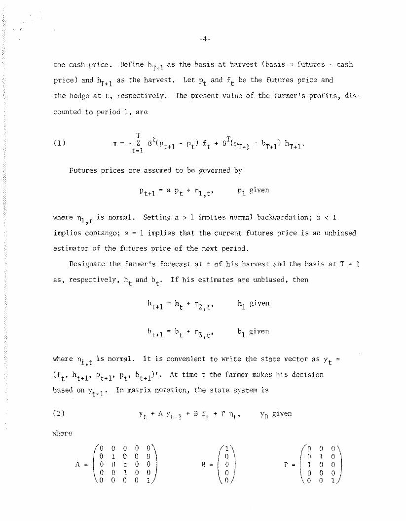
the cash price. Define bTcl as the hasis at harvest (basis = futures - cash

price) and as the harvest. Let pt and ft be the futures price and

the hedge at t, respectively. The present value of the farmer's profits, dis-

counted to period 1, are

Futures prices are assumed to be governed by

- Pt+l - a pt + %,tv p1 given

where is normal. Setting a > 1 implies normal backwardation; a < 1 , implies contango; a = 1 implies that the current futures price is an unbiased

estimator of the futures price of the next period.

Designate the farmer's forecast at t of his harvest and the basis at T + 1

as, respectively, ht and bt. If his estimates are unbiased, then

- ht+l - ht + q2,t7 hl given

- bt+l - bt + n3,t' bl given

where q. is normal. It is convenient to write the state vector as vt = 1 ,t

(ft' %+I> Pt+l' Pt' bt+l)t. At time t the farmer makes his decision

based on yt-l. In matrix notation, the state system is

( 2 1 Yt + A Vt-l + R ft + r 'it, v given 0

where

and Vt = VZ,~, n3,t 1 ' 'L N f O , E) . Equation (1 ) can be rewritten as

Current and future decisions do not depend on previous profits or the cur-

rent level of wealth, due to the assumptions of C4RA utility and a nonstochas-

tic interest rate. Define J(t, yt-l ) as the maximized expected value of the

utility of revenue from current and future hedginq and cash sales, discounted

to time t; the expectation is conditioned on vt-l. Tl~en J(t, vt-ll is the

solution to - -.

subject to ( 2 1 with yt-l given. The parameter k is the risk coefficient,

and the notation Et means the expectation conditioned on the infomation

available at t. In particular, J(1, yo) gives the expected utility, at the

beginning of the season, of the revenue from hedging and cash sales. 1 *

The function J(t, yt-l is of the form -st exp (-vt-l Wt yt/Z), and the

optimal hedge is given by ft = Gt Y ~ - ~ . The equations for calculating st, w i 2 and Gt are given in the Appendix. The problem differs from Jacobson's in

several minor respects. The presence of discounting leads to a trivial modi-

fication. In addition, n is linear in f, so it is necessary to check that

the first-order conditions do indeed imply a maximum and that the problem is

irell defined (the solution is bounded). These conditions are given in the

Appendix. Finallv, the difference equation (31 is written as a backward dif-

ference rather than a forward difference. This was done to make it more con-

venient to .write n.

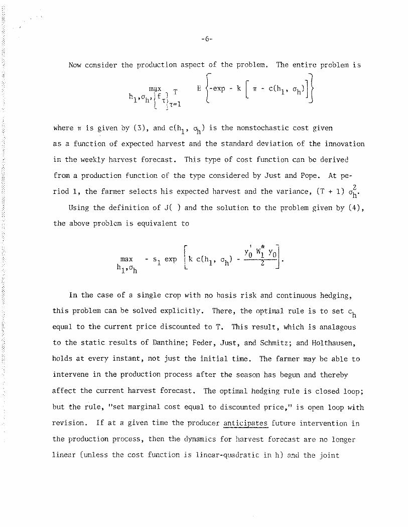
Now consider the production aspect of the problem. The entire problem is r 7

where n is given by ( 3 ) , and c(hl, oh) is the nonstochastic cost given

as a function of expected harvest and the standard deviation of the innovation

in the weekly harvest forecast. This type of cost function can be derived

from a production function of the type considered by Just and Pope. At pe-

riod l, the farmer selects his expected harvest and the variance, (T + l) o i .

Using the definition of J( ) and the solution to the problem given by ( 4 ) ,

the above problem is equivalent to

In the case of a single crop with no basis risk and continuous hedging,

this problem can be solved explicitly. There, the optimal rule is to set ch

equal to the current price discounted to T. This result, which is analagous

to the static results of Danthine; Feder, Just, and Schmitz; and Holthausen,

holds at every instant, not just the initial time. The farmer may be able to

intervene in the production process after the season has begun and thereby

affect the current harvest forecast. The optimal hedging rule is closed loop;

but the rule, "set marginal cost equal to discounted price," is open loop with

revision. If at a given time the producer anticipates future intervention in

the production process, then the dynamics for harvest forecast are no longer

linear (unless the cost function is linear-quadratic in h) and the joint

hedging-production problem does not fit the LEG mold. The introduction of

basis risk is discussed with the numerical example below.

Since W: is independent of the state, the first order condition for the * .

choice of h can be easily solved. Hohever, Wi is a function of oh so, for

higher dimensional problems, it is necessary to use numerical derivatives to

determine the optimal oh. Note that this parameter includes the uncertainty

due to the intrinsic variability of harvest and also due to forecast errors.

The farmer may alter oh by choice of production technology or by changing

the resources devoted to sampling and forecasting.

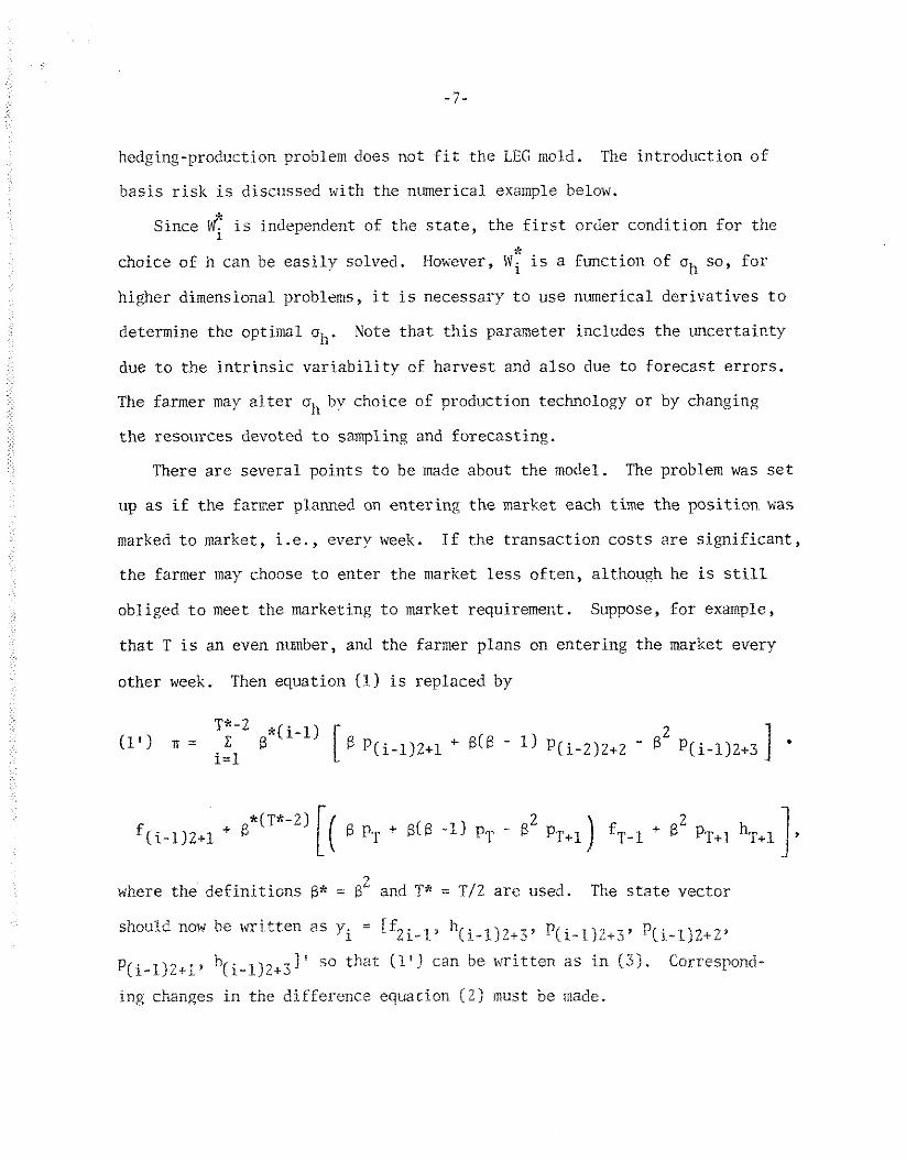
There are several points to be made about the model. The problem was set

up as if the farmer planned on entering the market each time the position was

marked to market, i-e., every week. If the transaction costs are significant,

the farmer may choose to enter the market less often, although he is still

obliged to meet the marketing to market requirement. Suppose, for example,

that T is an even number, and the farmer plans on entering the market every

other week. Then equation (1) is replaced by

2 where the definitions B* = B and T* = T/Z are used. The state vector

should now be written as y. = [fZi-L3 I h(i-l~~+3y p(i-l)2+37 P(i-l)~+~9

P(i-1)2+1 b(i-~)~+j 1 ' so that (1'1 can be written as in (3). Correspond-

ing changes in the difference equation ( 2 ) must be made.

Given an initial observation, yo, the farmer can repeatedly solve the

dynamic hedging problem varying the number of times he plans to enter the

market (T*). He can compare the expected utility and the moments of profits

under the different scenarios and select the optimal strategy. Entering the

market more often gives him greater flexibility and a higher expected revenue

but also higher transactions costs. Suppose that at t = 1 he decides to enter

the market every other week. At t = 2 this strategy calls for leaving his

initial hedge, f , unchanged until t = 3. However, f is not optimal at 1 I

t * 2 since he now has more recent information. It is a simple matter, using

the methods described in the next section, to recalculate the moments and

expected utility of profits, conditional on information available at t = 2,

under the assumption that ( I ) he adheres to his initial strategy or (2) he

departs from that strategy and revises his hedge at t = 2. This gives him the

information necessary to decide whether it pays to reenter the market.

The model was not written in its most general form. The matrices A and

C can depend on time; the algorithm in the Appendix shows them as time de-

pendent. Future prices may become either more or less volatile as harvest

approaches (Anderson and Danthine 1983b). In addition, the innovation in the

harvest forecast need not have constant variance. As previously suggested,

the farmer may be regarded as choosing a production technology which deter-

mines output variance or he may choose a sampling strategy which determines

the variance of the error of harrest forecast. Kith either interpretation,

2 E(n2 t) may be time dependent. Kumerical analysis will indicate the relative , importance of decreasing the variance of forecast error at different times in

the season. Since this depends in a complicated bay on all the parameters of

the problem, it is unlikely that analytic results can be obtained.

Inclusion of a constant in the state vector y allows an intercept to be

included in (2) and a constant and linear cost to be included in the profit

function. The latter permits an affine transactions cost to be included in

profits. No alteration in the algorithq is required. Under some circum-

stances, it may be desirable to include a cost which is quadratic in the

controls. This may arise if, for example, there is a control "fertilizer

application" which involves a quadratic adjustment cost and which changes the

expected harvest. Since the state vector is already augmented to include the

control(s), no change is needed in the algorithm.

Equation ( 2 ) indicates that only the current futures price contains infor-

mation about next period's futures price. This is an unnecessary restriction

and was adopted only for purposes of exposition. More generally, write

where zt is a vector of explanatory variables which may include current and

lagged prices; z becomes a component of the state y. The only necessary as-

sumptions are linearity and normality. The error rlt can be replaced by a

moving average term by suitable definition of zt.

The above modifications to the simple problem allow for a great deal of

flexibility and make the model useful.

Methods for Analyzing the Optimal Hedge

The previous section discussed the optimal hedging strategy conditional on the

parameters k , T*, and oh, at least the first two of which are determined by

the farmer. As a decision-making aid, this is incomplete. For example, the

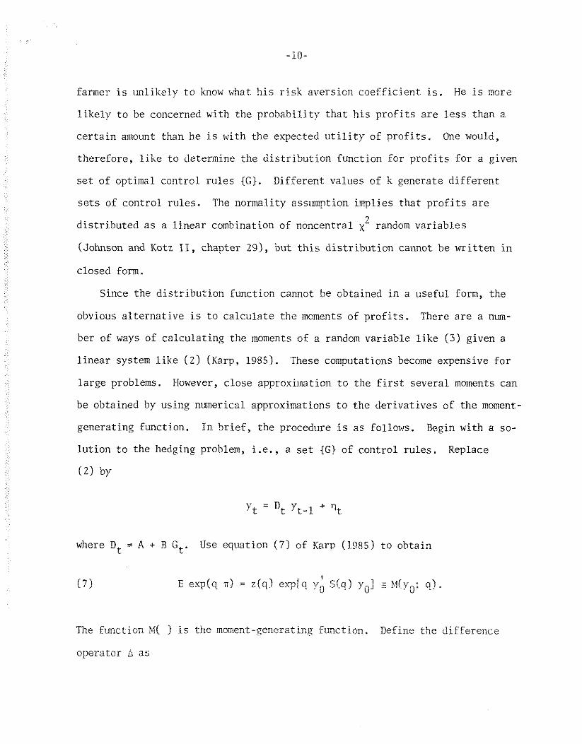
farmer is unlikely to know what his risk aversion coefficient is. He is more

likely to be concerned with the probability that his profits are less than a

certain amount than he is with the expected utility of profits. One would,

therefore, like to determine the distribution function for profits for a given

set of optimal control rules {G). Different values of k generate different

sets of control rules. The normality assumption implies that profits are

2 distributed as a linear combination of noncentral x random variables

(Johnson and Kotz 11, chapter 291, but this distribution cannot be written in

closed form.

Since the distribution function cannot be obtained in a useful form, the

obvious alternative is to calculate the moments of profits. There are a num-

ber of ways of calculating the moments of a random variable like (3) given a

linear system like ( 2 ) (Karp, 1985). These computations become expensive for

large problems. However, close approximation to the first several moments can

be obtained by using numerical approximations to the derivatives of the moment-

generating function. In brief, the procedure is as follows. Begin with a so-

lution to the hedging problem, i.e., a set {GI of control rules. Replace

(2) by

where Dt = A + B Gt. Use equation (7) of Karp (1985) to obtain

The function M( 1 is the moment-generating function. Define the difference

operator d as

n- l where r is a small positive number; A" 21 = A A M( ) , etc. Then the - nth

derivative of M with respect to q, evaluated at qo, is

The - nth moment of n is given by the - nth derivative of the moment-generating

function, evaluated at q = 0. Let q0 = 0, and use the fact that lil(yO, 0) = I;

approximate the nth - derivative of M with respect to q, evaluated at q = 0, as n

[A M(yO, O)]/rn. For example, approximating the first two moments of n

requires calculating the expression in (7) for two different values of q;

approximating the third and fourth moments requires making the calculation

four times. It is useful to approximate each moment using several values of r

to check for convergence. Exact calculation of the first moment is inexpen-

sive; this can be checked against the approximation to gauge the latter's

accuracy.

Having obtained a set of a finite number of moments of n , each set of

which corresponds to a different value of k (or T* or %), it is possible

to proceed. To avoid repetition, assume that the only question is to de-

termine the k that most accurately reflects the farmer's preferences. This

section suggests three methods of helping the farmer choose k. The first

method involves parameterizing on k and graphing the resulting mean-variance

trade-off. The second method uses a Chebvchev-type ineouality to obtain an

upper bound on the probability of prof~ts falling below a given level. The

third method uses the higher moments to obtain an approximation of the distri-

bution function for profits. This can then be used to obtain the expected

value of a given function of profits or the probability that profits are below

a given level.

The first method involves parameterizing on k to obtain various sets of

control rules and corresponding pairs of mean and variance of profits. The

farmer chooses the preferred mean-variance trade-off. Parameterizing on k

does not - sweep out the mean-variance frontier because the maximand is not a

mean-variance criterion. For small values of k, the two criteria are similar

and give similar results. This is not so for large values of k. Numerical

experiments show that for large k further increases in risk aversion lead to a

decrease in expected profits and an increase in the variance. This is not

surprising--for large k, the third and higher moments of profits assume

increasing importance

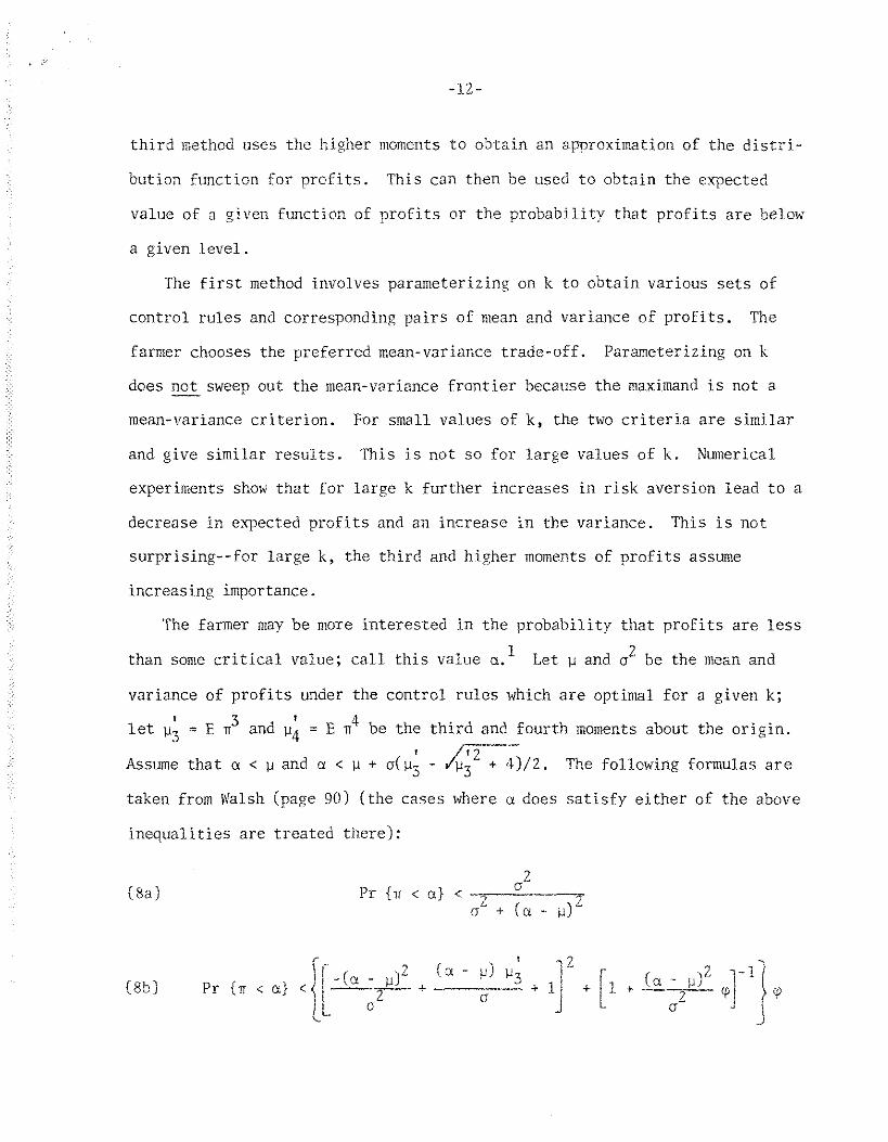
The farmer may be more interested in the probability that profits are less

2 than some critical value; call this value a.' Let p and o be the mean and

variance of profits under the control rules which are optimal for a given k; 1 3 4

let u3 = E II and pi = E n be the third and fourth moments about the origin.

Assume that o < p and o < u + o(u; - 2 . The following formulas are

taken from Malsh (page 90) (the cases where a does satisfy either of the above

inequalities are treated there):

0 2

[%a) Pr Cn < a) < 0" ((a - DlZ

1

( a - PI u3 Pr i n < a) <I[+ o + u -11 'F isbl

i u

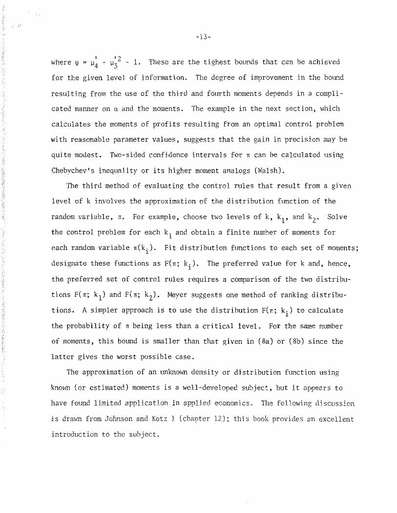
1 where ip = p l2 - 1. These are the tighest bounds that can be achieved 4 - p3

for the given level of information. The degree of improvement in the bound

resulting from the use of the third and fourth moments depends in a compli-

cated manner on n and the moments. The example in the next section, which

calculates the moments of profits resulting from an optimal control problem

with reasonable parameter values, suggests that the gain in precision may be

quite modest. Two-sided confidence intervals for n can be calculated using

Chebychev's inequality or its higher moment analogs (Walsh).

The third method of evaluating the control rules that result from a given

level of k involves the approximation of the distribution function of the

random variable, n. For example, choose two levels of k, kl, and k2. Solve

the control problem for each ki and obtain a finite number of moments for

each random variable n(ki). Fit distribution functions to each set of moments;

designate these functions as F(x; ki). The preferred value for k and, hence,

the preferred set of control rules requires a comparison of the two distribu-

tions F(n; kl) and F(n; k2). Meyer suggests one method of ranking distribu-

tions. A simpler approach is to use the distribution F(n; ki) to calculate

the probability of n being less than a critical level. For the same number

of moments, this bound is smaller than that given in (8a) or (8b) since the

latter gives the worst possible case.

The approximation of an unknown density or distribution function using

known (or estimated) moments is a well-developed subject, but it appears to

have found limited application in applied economics. The following discussion

is dram from Johnson and Kotz I (chapter 12) ; this bock provides an excellent

introduction to the subject.

It is convenient to standardize the random variable n. Replace n by

rl = (n - p)/a, so ?; has 0 mean and unit variance. Write the - ith central mo-

ment as )i. i > 2. The following quantities play an important role: Bl = 1' -

(p3/d)2 is a measure of skewness; and B2 = p4/a4 is a measure of excess or

kurtosis. Given the first four moments about the origin of the original ran-

dom variable n, it is straightforward to obtain the central moments of the

standardized variable ?i and, hence, and BZ. Hereafter, it is understood

that El and B2 give the skewness and kurtosis of I?.

The Pearson system provides one method of using the moments to fit a dis-

tribution. For a random variable x, suppose that the probability density p(x)

satisfies the differential equation

The form of the solution to this equation depends on the values of the pa-

rameters co, cl, cZ, and c3. These parameters have a simple relation to the

moments of the random variable and, hence, to El and B2. Calculation of El

and BZ and inspection of a chart (Johnson and Kotz I, Figure 1, p. 14) deter-

mine to which type of distribution the moments correspond. These types include

the beta, gamma, and T distributions. Calculation of the parameters co, cl,

C2' and c permits calculation of the parameters of that distribution. If the 3

distribution is of a common type, it is possible to use tables to determine

the probability that n (and, hence, n ) falls below a given level. For less com-

mon types of distributions, numerical integration may be used,

Various types of expansions provide alternatives to the Pearson system.

The idea is to express the unknom density (that of $1 hith known (or esti-

mated? moments as a function of some tractable density, f ( ). One of the most

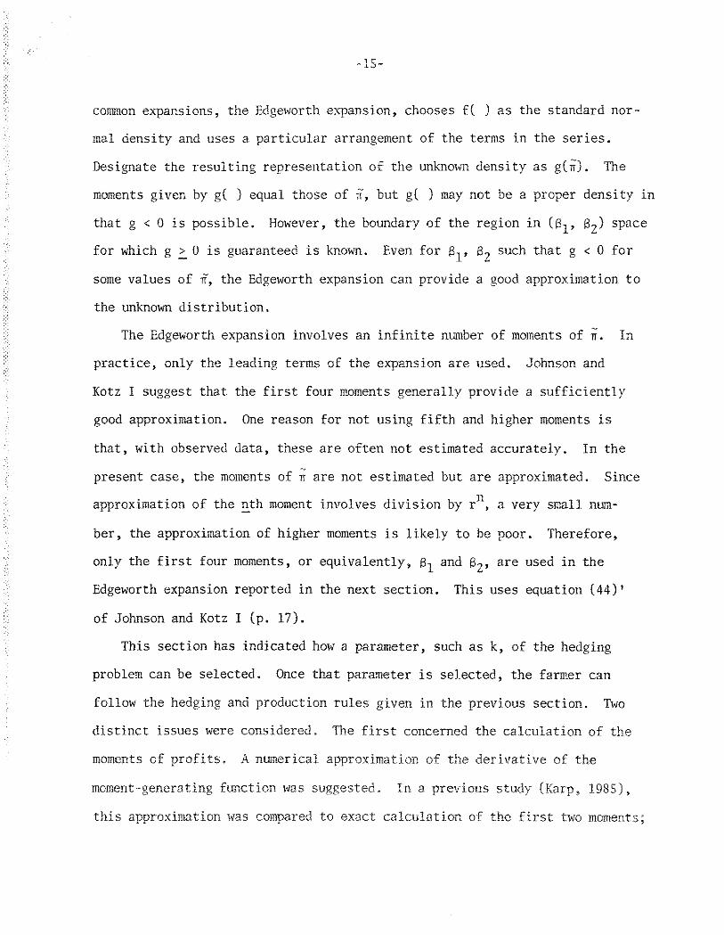
common expansions, the Edgeworth expansion, chooses f( ) as the standard nor-

mal density and uses a particular arrangement of the terms in the series.

Designate the resulting representation of the unknokn density as g(?;). The

moments given by g( ) equal those of <, but g( may not be a proper density in

that g < 0 is possible. However, the boundary of the region in (B1, B2) space

for which g - > 0 is guaranteed is known. Even for Bl, B2 such that g < 0 for

some values of I?, the Edgeworth expansion can provide a good approximation to

the unknown distribution,

The Edgeworth expansion involves an infinite number of moments of ?;. In

practice, only the leading terms of the expansion are used. Johnson and

Kotz I suggest that the first four moments generally provide a sufficiently

good approximation. One reason for not using fifth and higher moments is

that, with observed data, these are often not estimated accurately. In the

present case, the moments of are not estimated but are approximated. Since

approximation of the - nth moment involves division by rn, a very small num-

ber, the approximation of higher moments is likely to be poor. Therefore,

only the first four moments, or equivalently, B1 and B2, are used in the

Edgeworth expansion reported in the next section. This uses equation (44) '

of Johnson and Kotz I (p. 17).

This section has indicated how a parameter, such as k, of the hedging

problem can be selected. Once that parameter is selected, the farmer can

follow the hedging and production rules given in the previous section. Two

distinct issues were considered. The first concerned the calculation of the

moments of profits. numerical approximation of the derivative of the

moment-generating function was suggested. In a previous study (Karp, 1985),

this approximation was compared to exact calculation of the first two moments;

the results were encouraging. The second issue concerned how the moments

should be used. Three possibilities were suggested: (1) derive the mean-

variance trade off, (2) obtain an upper bound on the probability of a low

level of profits by means of a Chebychev-type inequality, and (3) approximate

the unknown distribution. The third alternative can be accomplished usine the

Pearson system or an expansion such as the Edgeworth expansion. The next sec-

tion applies the methods of this and the previous section.

Illustration of the Methods

A simple example illustrates the methods of the previous two sections. The

parameter values used are of a reasonable order of magnitude but do not

represent detailed statistical analysis. Wheat yield data (U. S. Economic

Research Service) for the United States (1967-1983) suggest expected harvest

of 32.32 bushels per acre with a sample variance of 8.2. The length of the

season, T, was set at 16 weeks; and the variance of the weekly innovation in

harvest forecast was taken to be 8.2/16 = .51. Using 1983 weekly data

(Chicago Board of Trade) (June 1-September 41, the sample variances of the

weekly change in futures price and basis were, respectively, .021 and .004.

The initial futures price and expectation of the harvest basis were taken to

be 3.54 and .057 dollars per bushel. The weekly discount rate, 6, was set

at .998, implying an annual interest rate of 10 percent. The covariances of

p, b, and h were set at 0. These parameter values are referred to as base

values. The regression of pt on ptel using 1983 data implied a coefficient of

a = .94; choosing a to solve p a 1 l 6 = p17 gave a = 1.002. The results be:ow,

except where indicated otherwise, use the intermediate value a = -98. This

implies that price is expected to fall.

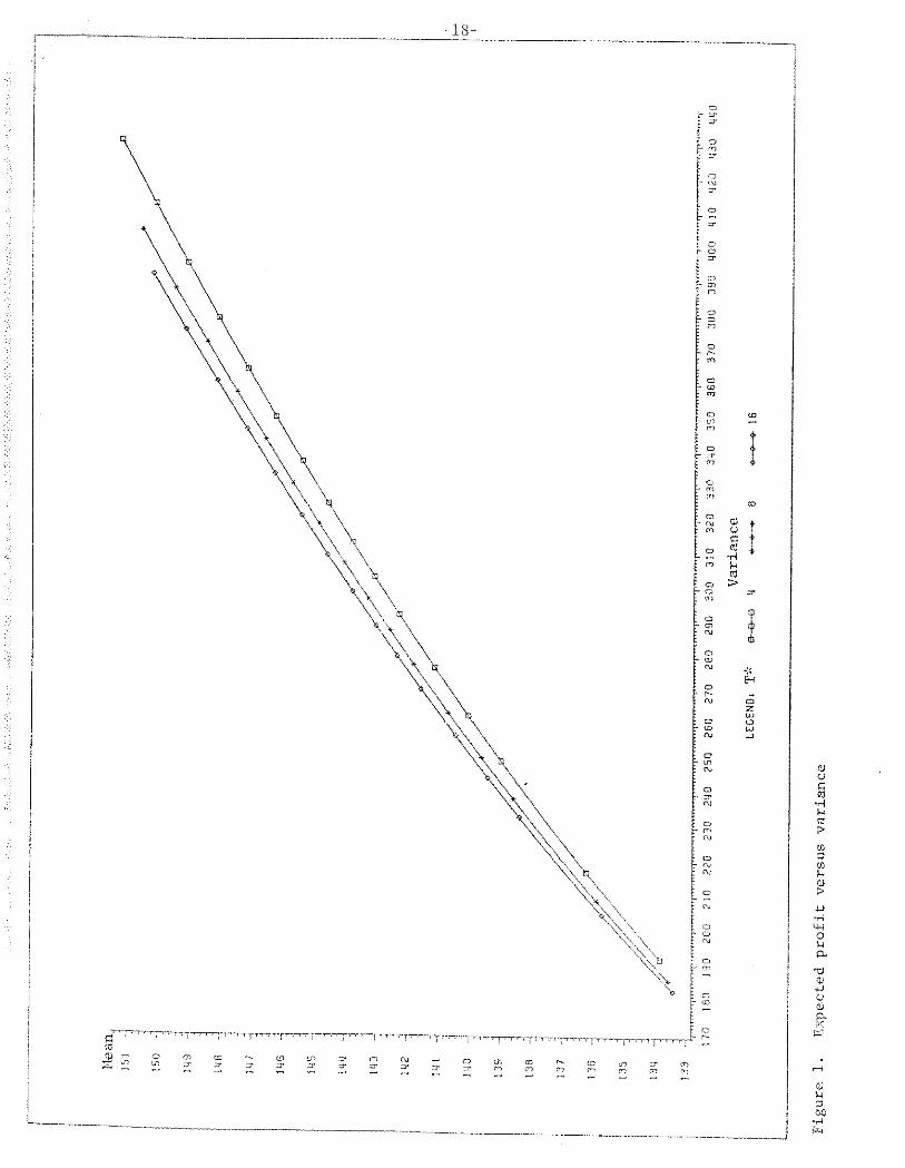
In order to indicate the advantage of entering the market frequently, the

optimal hedging problem was solved for 16 values of k in the range (.0025, .12)

under the assumption that the farmer enters the market (I) every week, (2) ev-

ery second week, and (3) every fourth week. The mean and variance of profits

were calculated in each case, and the result is shown in figure 1. The three

curves give the mean-variance trade-off for the three strategies. Since

transactions costs were set at 0, the farmer does better for every level of

risk aversion by entering the market 16 times. The inclusion of transactions

costs may cause the relative positions of the curves to change, and the curves

may cross. In the latter case farmers with different levels of risk aversion

and the same transaction costs will not only make different hedges but will

change their hedge with different frequency.

For the results shown, a lower level of risk aversion corresponds to a

higher level of expected profits and a higher variance. As mentioned in the

previous section, it is possible for the mean-variance graph to be decreas-

ing. This occurs at large values of k. The graph indicates that the location

of the mean-variance point is more sensitive to changing the nmber of times

the farmer hedges when the level of risk aversion is small. This occurs be-

cause, for small levels of risk aversion, the farmer is more willing to take

advantage of the opportunity for speculation.

The mean-variance trade-off offers the farmer some help in choosing his

preferred levels of k and T* and, thus, his optimal hedging and production

rules. Supplementary information is obtained by considering the probability

6 [associated with each level of k ) that profits fall below a given level a.

The previous section discussed methods of putting a bound on 6 and of obtain-

ing an approximation of the distriburion of n and, hence, an approximation

of 5. To illustrate these methods, suppose that the fanner has decided to

enter the market four times. He now chooses k on the basis of the mean and

variance of profits and of the probability, 5, of profits falling below

a = $120. Table 1 provides him with this last piece of information. The

first column gives k; columns 2 and 3 give, respectively, the third and fourth

moment of the standardized random variable, G . For all levels of k, the

distribution of profits is skewed to the left. Since p4 > 3, the value of the

fourth moment for the standard normal, the tails are "someiihat thick." The

fourth and fifth columns give and 52, the upper bounds on the probability

that profits are less than $120 per acre using, respectively, the first two

and the first four moments /(8a) and (8b), respectively].

2 The coefficients of the Pearson system were calculated using Bl = p3 and

B2 = p4. For all values of k, the results indicate that is distributed (ap-

proximately) as a beta. The parameters of the distribution were calculated

from the coefficients of the Pearson system, and the SASS function PROBBETA was

then used to obtain the probability that n < 120. This is reported as in

column 6. Column 7 gives cS4, the probability that n < 120, obtained from the

Edgeworth expansion

The table indicates that the use of the third and fourth moments in the

Chebychev-type inequalities results in an improvement in the bound of only

1 percent to 3 percent (compare and b2). However, the approximation tech-

niques suggest that 6 is only 25 percent to 30 percent of the upper bound. It

is encouraging that the two approximation techniques give comparable estimates.

This suggests (biit, of course, does not prove) that the approximations are

close to the true density.

The upper bound of 6, given by or IS^, and the estimate of 6, given by

63 or 54, provide different pieces of information; their incorporation into

Table 1. Variation in the Distribution of Profits

"3 = skewness for standardized random variable.

~4 = kurtosis for standardized random variable.

61 = upper bound on PrCn < 120) using (8a).

62 = upper bound on Prin < 120) using (8b).

63 = estimate of Pr{n < 120) using beta distribution.

64 = estimate of Pris < 120) using Edgeworth expansion.

the decision-making process is a matter of judgment. If the true model for

the stochastic processes Mere known and if the criterion were literally

"safety first," then it would be appropriate to use the upper bound of 6 to

evaluate the control rules. In practice, the parameters of the stochastic

processes are estimated; and the decision-maker is likely to regard the in- - -

equality 6 - < 6, 6 given, as a desirable characteristic rather than as a

precise constraint. On both of these counts, it is more reasonable to seek a

reliable estimate of 6 rather than its upper bound. Table 1 gives an indi-

cation of the extent to which the use of an upper bound rather than an esti-

mate of 6 can lead to overly conservative behavior.

The table also shows that, as the hedger becomes more risk averse, the

distribution becomes slightly less skewed. As he becomes more risk averse,

the probability that profits are less than 120 increases. The decrease in

expected profits more than offsets the decrease in variance. The farmer may

find it strange that an increase in his risk aversion is associated with an

increase in the probability of falling below some critical level of profits.

Different choices of CY or k or different parameters in the control problem

may reverse the result so that increases in risk aversion could lead to a

decrease in the probability of profits being less than a. The CARA utility

function attaches a specific meaning to "risk aversion," whereas the same term

means a host of things to most people.

The accuracy of the results in table 1 is conditioned on the accuracy of

the approximations of the higher moments of profits. Recall that these are

obtained as nmerical derivatives to the moment-generating function, For each

level of k, the first four moments were approximated using 10 values of the

step size r, ranging from 5 x to 4 x the first moment was also

calculated exactly as a gauge of accuracy. As expected, the approximations

for the lower moments are more stable than those of the higher moments. The

approximation of the first moment is extremely stable. It varies by less than

.O1 percent and is within .01 percent of the true value. The approximations

of the second and third moments vary by less than 1 percent. The approxima-

tion for the fourth moment is much less stable, varying by almost 10 percent.

In addition, the resulting approximations of 6 using r close to 4 x 10'~ are

nonsensical, falling outside the range (0, 1). However, for larger r, e.g.,

5 r E ( 5 x 4 x 10' ), the approximations of the fourth moment are very

stable; and the resulting approximations 6' and 63 are even more so. Table 1

- 4 reports results using step size r = 5 x 10 . This discussion indicates the importance of experimenting with different step sizes. If r is too large, the

derivative is not approximated well.; if r is too small, numerical problems

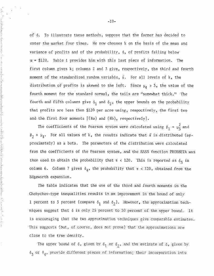
4 arise because the approximation to the fourth moment requires r . A previous section mentioned that, with zero basis risk and continuous

hedging, the marginal cost of expected harvest is set equal to the discounted

price. With the discount rate used above, this gives pl - bl = 1.02979 ch( 1.

Table 2 indicates how the rule is altered for moderate basis risk.' The

interest rate still predominates. It is apparent that an increase in risk

aversion can lead to an increase or decrease in planned harvest (since c is

convex); however, the effect of risk aversion on planned harvest is small.

In the continuous time mode!. with no discounting and no basis risk, the

optimal hedge is expected to increase over time if the ratio of the absolute

value of the percentage of expected change in price to the level of risk aver-

sion is "small"; if the ratio is large, the hedge is expected to increase. 3

Table 2. The Optimal Choice of Expected Harvest, hl

k Equation t o determine h,

Nmerical analysis indicates that this also holds in discrete time with dis-

counting and basis risk. That is, the hedge is expected to rise (fall) if

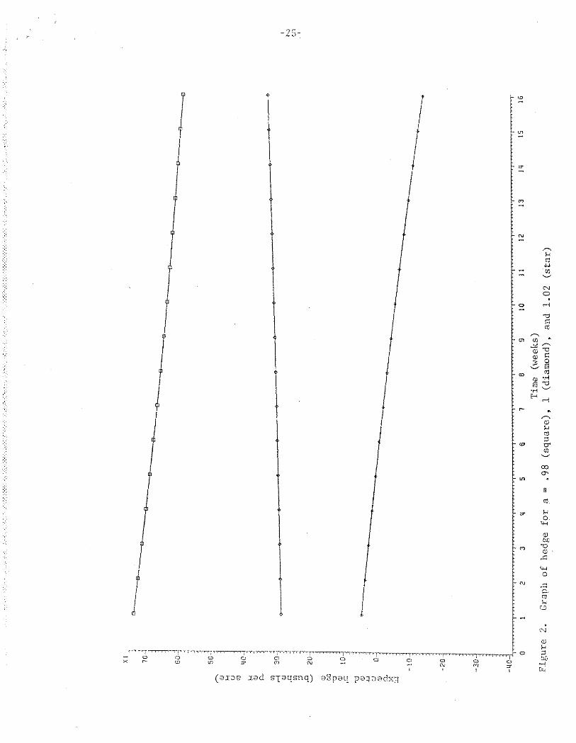
E / ~ t + l - ptl/ptk = I1 - a//k is small (large). Figure 2 graphs the expected hedge for a = .98, 1, 1.02, and k = .0978.

The graph is obtained using the optimal control rules with the equations of

motion for p, b, and h and setting all random variables equal to their ex-

pected values. For the first and last values, la - ll/k = .204 is large, and the

hedge is expected to fall. For the intermediate case, la - ll/k = 0 is

small, and the hedge is expected to rise. In the case where price is expected

to fall (a = .98), the hedger initially sells contracts and proceeds to buy

them back over the season. He ends the season with a short position of ap-

proximately twice his expected cash crop. In the third case (a = 1.021, price

is expected to rise. The hedger initially sells a few contracts as a hedge

against an unexpected drop in price. He then proceeds to buy contracts, fin-

ishing the season in a long position. For both of these cases, the hedger's

behavior is motivated by speculation on expected price change; in neither case

does his hedge approach expected harvest.

The important point is that, although the level of the hedge depends on

whether price is expected to increase or decrease, the expected direction of

change in the hedge depends on a comparison between the magnitude of the ex-

pected price change and the degree of risk aversion. Wen the price is not

expected to change (a = 11, the farmer hedges slightly less than expected pro-

duction. As the season progresses, his hedge converge.: to expected production.

The exampie can also be used to indicate the value of entering the futures

market. In the absence of hedging, with a = .48 and the base value parameters,

the expected value of revenue per acre is $79.68; and the standard deviation

-

." -

= -

"7 -

m - ,-. Fi m U - u] - w

N 0

51 T' a C m ,-.

m u ] ' 3 - aJ g ,5 - S

m aJ -4

.5 w t i

a

aJ Fi m s ii- u] -

m a

U1

I1

n

= &' 0

W

aJ bc

m I) S W 3

.z c& z r, - N

!lJ &'

0 3 Ci .i j,

is $17.41. With the same parameter values and setting k = .0078, the optimal

hedge results in expected profits of $143.11 with a standard deviation of

$17.41. The advantage of hedging is so pronounced because a j. 1, which

implies the possibility for speculative profits.

Conclusion

This paper has described and illustrated a practical technique for determining

optimal hedges. The method uses the LEG control problem. It requires assump-

tions which are analogous to those underlying the more common mean-variance

optimization problem which uses quadratic programming. Its advantage over the

mean-variance approach is that it incorporates dynamics (anticipated revision

of hedges).

The solution of the optimization problem is straightforward. Varying pa-

rameters, such as k, the degree of risk aversion, or T*, the number of times

the farmer enters the market, generates families of optimal control rules.

The interesting practical problem is to determine which of these rules should

be followed, i.e., to determine the best k or T*. Several suggestions were

made, all of which require calculation of the moments of profits. Perhaps the

most promising involves approximating the distribution of profits either by

using the Pearson system or by some type of expansion. The approximate dis-

tributions provide the decision-maker with more relevant information than do

the Chebychev-type inequalities, which are extremely conservative.

The techniques discussed in this paper were motivated by the hedging and

pro&wtion problem* However, it is clear that the same methods can be used

for any situation that conforms to the assumptions of the LEG control problem,

Appendix

The LEG Algorithm

The following definitions are used

, - Gt = -(B kl' B )'I R; it At t t t

- -1 ' w t =wt - w t rt(ql+ r;wt rt) rt wt 1 - w," = At [iVt - it B~(B; 4 Rt )-I B; kt] At.

The difference equations are

The second-order condition is that B; wt Bt be negative definite for 1

all t. In addition, I + Ct rt Wt rt must be positive definite to insure that expected utility is bounded.

Footnotes

l~he confidence intervals discussed in this section use the moments

of n. Other statistics, such as the semivariance, can also be used (Berck,

1982). For the problem at hand, the moments are easier to calculate.

'Table 2 is an approximation. It ignores the fact that the coefficients

on p and b differed by at most '001 percent in absolute value. This differ-

ence is due to the fact that the futures price and basis follow different

stochastic processes, so the current cash price is not exactly a sufficient

statistic for the choice of hl.

3 . . This IS a paraphrase of Remark 4 in Karp (1986). For some values of

the above-mentioned ratio, the expected hedge is not monotonic in time; for

very large values of the ratio and a > 1, the hedge is expected to increase.

References

iXnderson, R. W., and J. Danthine. "Cross Hedging." J. Polit. Econ.

89(1981):1182-196.

. "Hedger Diversity in Futures h*arkets." Econ. J. Y3( 1983a) :370-89.

. "The Time Pattern of Hedging and the Volatilitv of Futures Prices." Rev. Econ. Stud. 50(1983b):249-66.

Ratlin, C. A. "Production IJnder Price Uncertainty with Imerfect Time Hedging

Opportunities in Futures Markets." Southern Econ. J. 49(1984):681-92

Berck, Peter. "Portfolio Theory and the Demand for Futures: The Case of

California Cotton." Amer. J. Agr. Econ. 63(1981):466-74.

. "Using the Semivariance to Estimate Safety-First Rules." Amer. - J. Agr. Econ. 64(1982):298-300.

Bray, M. "Futures Trading, Rational Expectations and the Efficient klarkets

Hypothesis." Econometrica 49(1981):575-96.

Chicago Board of Trade. Annual Cash and Futures Data: Grains, Forest Products

Enerjy," 1983.

Cox, J. C., J. E. Ingersoll, Jr., and S. A. Ross. "The Relation Between For-

ward Prices and Futures Prices." J. Financial Econ. 9(1981):321-46.

Danthine, J. "Information, Futures Prices, and Stabilizing Speculation."

J. Econ. Theorv 17(1978):79-98.

Feder, G., R. Just, and A. Schmitz. "Futures Varkets and the Theorv of the

Firm IJnder Price Uncertainty." Quart. J. Econ. 95(lo80):317-28.

Wildreth, C . "An Expected iitility Yodel of Grain Storage and I i edg in~ by

Farmers." Technical Bulletin 321. Apricu?tural Experiment Station, Uni-

versity of blinnesota, 1979.

Ho, T. "Intertenporal Commodity Futures Hedging and the Prodtiction Decision."

J. of Finance 39(1984):351-75.

kIolthausen, D. M. "Hedging and the Competitive Firm Under Price lincertaintv."

her. Econ. Rev. 69(1979):989-95.

Jacobson, D. H. "Optimal Stochastic Linear Systems with Exponential Per-

formance Criteria and Their Relation to Deterministic Differential

Games." IEEE Transactions on .&utomatic Control AC-18 (1973) : 124-31.

Johnson, Norman L., and Samuel Kotz. Distributions in Statistics, Contint~ous

Univariate Distributions, I and TI. New York: John \%Tiley and Sons, 1970.

Just, Richard E., and R. D. Pope. "Stochastic Specification of Production

Functions and Economic Implications." 3. Econometrics 7(1979):67-86.

Karp, Larry. "bnamic Hedqing with Uncertain Production." Working Pauer

No. 371. Department of Agricultural and Resource Economics, University of

California, Berkeley, 1986,

. "Higher Moments in the Linear-Quadratic-Gaussian Problem." J. Econ.

Dynamics and Control 9(1985):41-54.

Marcus, A. J., and D. M. Modest. "Futures Markets and Production Decisions."

J. Polit. Econ. 92(1984):409-26.

McKinnon, R. I. "Futures Markets, Buffer Stocks and Income Stability for

Primary Producers." J. Polit. Econ. 75(1967):84-861.

bleyer, Jack. "Choice Among Distributions." J. Econ. Theory 14(1977) :326-36.

Nelson, Ray. "Forward and Futures Contracts." her .I. A??. Econ. 67(l985):

15-23,

Peck, Anne E. "Hedging and Income Stability: Concepts, Im,ications, and an

Example." Am?. .J. Aqr. Econ. 57(1975): 410-19.

Rolfo, J. "C??tirnal Hedging ilnder Price and Quantity Uncertainty: The Case of

a Cocoa Producer." 3. Polit. Econ. 88(19801:100-15.

U. S. Economic Research Service. Wheat Outlook and Situation, Washington,

D. C., 1985.

Walsh, J. Handbook of Nonparameteric Statistics. New York: D. Van Nostrand

Company, Inc., 1962.