Selection of Best Sorting Algorithm for a Particular

Problem

Thesis submitted in partial fulfillment of the requirements for the award of

degree of

Master of Engineering

in

Computer Science & Engineering

By

Aditya Dev Mishra

(80732001)

Under the supervision of

Dr. Deepak Garg

Asst. Professor

CSED

COMPUTER SCIENCE AND ENGINEERING DEPARTMENT

THAPAR UNIVERSITY

PATIALA – 147004

JUNE 2009

i

ii

iii

ABSTRACT

Sorting is the fundamental operation in computer science. Sorting refers to the

operation of arranging data in some given order such as increasing or decreasing, with

numerical data, or alphabetically, with character data.

There are many sorting algorithms. All sorting algorithms are problem specific. The

particular Algorithm one chooses depends on the properties of the data and operations

one may perform on data. Accordingly, we will want to know the complexity of each

algorithm; that is, to know the running time f (n) of each algorithm as a function of

the number n of input elements and to analyses the space requirements of our

algorithms. Selection of best sorting algorithm for a particular problem depends upon

problem definition. Comparisons of sorting algorithms are based on different

scenario. We are comparing sorting algorithm according to their complexity, method

used like comparison-based or non-comparison based, internal sorting or external

sorting and also describe the advantages and disadvantages. One can only predict a

suitable sorting algorithm after analyses the particular problem i.e. the problem is of

which type (small number, large number, repeated value).

iv

TABLE OF CONTENTS

CERTIFICATE............................................................................................................ i

ACKNOWLEDGEMENT.......................................................................................... ii

ABSTRACT............................................................................................................... iii

TABLE OF CONTENTS........................................................................................... iv

LIST OF FIGURES...................................................................................................vii

LIST OF TABLES....................................................................................................viii

1. INTRODUCTION....................................................................................................1

1.1 Introduction......................................................................................................1

1.2 Sorting..............................................................................................................3

1.3 Classification of Sorting Algorithms...............................................................3

1.4 Method of sorting.............................................................................................5

1.5 Why Sorting.....................................................................................................6

1.6 Organization of Thesis.....................................................................................7

2. SOME FUNDAMENTAL SORTING ALGORITHMS......................................8

2.1 Insertion Sort....................................................................................................8

2.2 Bubble Sort.......................................................................................................9

2.3 Selection Sort.................................................................................................10

2.4 Bucket Sort.................................................................... ................................11

2.5 Quick Sort......................................................................................................12

2.6 Radix Sort......................................................................................................14

2.7 Counting Sort.................................................................................................16

3. SOME ADVANCED SORTING ALGOITHMS................................................18

3.1 Proxmap Sort..................................................................................................18

3.2 Merge Sort......................................................................................................19

v

3.3 Shell Sort........................................................................................................20

3.4 Library Sort....................................................................................................20

3.5 Heap Sort........................................................................................................21

3.6 Gnome Sort.....................................................................................................23

3.7 Stack Sort........................................................................................................23

3.7.1 The distribution phase of Stack Sort.....................................................24

3.7.2 The collection phase of Stack Sort........................................................25

3.8 Deqsort............................................................................................................26

3.8.1 The distribution phase of DeqSort........................................................26

3.8.2 The collection phase of DeqSort...........................................................27

3.9 Minimax Sort...................................................................................................28

3.9.1 The distribution phase of MinMax Sort.................................................29

3.9.2 The collection phase of MinMax Sort....................................................29

3.10 A New Sorting Algorithm.............................................................................30

4. SORTING NETWORK

4.1 Bitonic Sort.....................................................................................................32

4.2 Odd-Even Sorting Network............................................................................34

5. PROBLEM STATEMENT...................................................................................35

5.1 Problem Statement.........................................................................................35

5.2 Justification....................................................................................................35

5.3 Explanation....................................................................................................36

6. RESULTS & DISCUSSION.................................................................................37

6.1 Problem Definition and Sorting Algorithms..................................................37

6.2 Strength and Weakness..................................................................................38

6.3 Comparison of Various Sorting Algorithms..................................................39

6.3.1 Comparison of Comparison Based Sorting Algorithms.......................40

6.3.2 Comparison of Non Comparison Based Sorting Algorithms...............41

vi

7. CONCLUSION......................................................................................................43

ANNEXURES

I. References........................................................................................................46

II. List of publications............................................................................................49

vii

LIST OF FIGURES

Figure 2.1: Example of Insertion Sort............................................ ..............................8

Figure 2.2: Example of Selection Sort.........................................................................10

Figure 2.3: Example of Bucket Sort............................................................................ 11

Figure 2.4: Example of Quick Sort..............................................................................13

Figure 2.5 Example of Radix Sort................................................................................15

Figure 2.6 Example of Counting Sort..........................................................................16

Figure 3.1: Example of Proxmap Sort......................................................................... 18

Figure 3.2: Example of Merge Sort..............................................................................19

Figure 3.3: Example of Shell Sort................................................................................20

Figure 3.4: Example of Heap Sort................................................................................22

Figure 4.1: Example of Biotonic Sort..........................................................................32

viii

LIST OF TABLES

Table 6.1 Problem Definition and Sorting Algorithm................................................37

Table 6.2 Strength and Weakness..............................................................................39

Table 6.3 Comparison of comparison based sorting algorithms................................40

Table 6.4 Comparison of non-comparison based sorting algorithms.........................41

ix

1

CHAPTER 1

INTRODUCTION

1.1 Introduction

There are many fundamental and advance sorting algorithms. All sorting algorithm are

problem specific means they work well on some specific problem and do not work well

for all the problems. All sorting algorithm apply to specific kind of problems. Some

sorting algorithm apply to small number of elements, some sorting algorithm suitable for

floating point numbers, some are fit for specific range ,some sorting algorithms are used

for large number of data, some are used if the list has repeated values. We sort data either

in numerical order or lexicographical, sorting numerical value either in increasing order

or decreasing order and alphabetical value like addressee key.

One of the fundamental problems of computer science is ordering a list of items. There is

a plethora of solutions to this problem, known as sorting algorithms. Some sorting

algorithms are simple and intuitive, such as the bubble sort. Others, such as the quick sort

are extremely complicated, but produce lightning-fast results. The common sorting

algorithms can be divided into two classes by the complexity of their algorithms. There is

a direct correlation between the complexity of an algorithm and its relative efficiency.

Algorithmic complexity is generally written in a form known as Big-O notation, where

the O represents the complexity of the algorithm and a value n represents the size of the

set the algorithm is run against. The two classes of sorting algorithms are O(n2), which

includes the bubble, insertion, selection, and shell, sorts; and O(n log n) which includes

the heap, merge, and quick sort.

Since the dawn of computing, the sorting problem has attracted a great deal of research,

perhaps due to the complexity of solving it efficiently despite its simple, familiar

statement. It is not always possible to say that one sorting algorithm is better than another

sorting algorithm. Performance of various sorting algorithm depend upon the data being

sorted. Sorting is used in many important applications such that there has been an

abundance of performance analysis. However, most previous research is based on the

2

algorithm‟s theoretical complexity or their non-cached architecture. As most computers

today contain cache, it is important to analyze them based on their cache performance.

Quick sort was determined to be a good sorting algorithm in terms of average theoretical

complexity and cache performance.

Sorting is one of the most important and well-studied problems in computer science.

Many good algorithms are known which offer various trade-offs in efficiency, simplicity,

memory use, and other factors. However, these algorithms do not take into account

features of modern computer architectures that significantly influence performance. A

large number of sorting algorithms have been proposed and their asymptotic complexity,

in terms of the number of comparisons or number of iterations, has been carefully

analyzed [1]. In the recent past, there has been a growing interest on improvements to

sorting algorithms that do not affect their asymptotic complexity but nevertheless

improve performance by enhancing data locality [3, 6, 21].

Sorting is a fundamental task that is performed by most computers. It is used frequently

in a large variety of important applications. Database applications used by schools, banks,

and other institutions all contain sorting code. Because of the importance of sorting in

these applications, dozens of sorting algorithms have been developed over the decades

with varying complexity. Slow sorting methods such as bubble sort, insertion sort, and

selection sort have a theoretical complexity of O (n2). Even though these algorithms are

very slow for sorting large arrays, the algorithm is simple, so they are not useless. If an

application only needs to sort small arrays, then it is satisfactory to use one of the simple

slow sorting algorithms as opposed to a faster, but more complicated sorting algorithm.

For these applications, the increase in coding time and probability of coding mistake in

using the faster sorting algorithm is not worth the speedup in execution time. Of course,

if an application needs a faster sorting algorithm, there are certainly many ones available,

including quick sort, merge sort, and heap sort. These algorithms have a theoretical

complexity of O (n log n). They are much faster than the O (n2) algorithms and can sort

large arrays in a reasonable amount of time. However, the cost of these fast sorting

methods is that the algorithm is much more complex and is harder to correctly code. But

3

the result of the more complex algorithm is an efficient sorting method capable of being

used to sort very large arrays.

1.2 Sorting

One of the most common applications in computer science is sorting, through which data

are arranged according to their values.

Let A be a list of n elements A1,A2……………AN in memory. Sorting of A means the

operation of rearranging the contents of A so that they are increasing in order

(numerically or lexicographically), so that

A1 <=A 2< =A3 < = A4…………<=AN.

Since A has n elements, there are n! Ways that the contents can appear in A. these ways

correspond to the n! Permutation of 1, 2, 3……..n. accordingly, each sorting algorithm

must take care of these n! Possibilities.

1.3 Classification of Sorting Algorithms

( i ) Based on data size

Sorts are generally classified as either external sorting or internal sorting. An internal sort

is the sort in which all the data are held in the primary memory during the sorting

process. An external sort uses primary memory for the data currently being sorted and

secondary storage for any data that will not fit in the primary memory.

( ii) Based on information about data

Comparison based sorting: A comparison based algorithm orders a sorting array by

weighing the value of one element against the value of other elements. Algorithms such

as quick sort, merge sort, heap sort, bubble sort, and insertion sort are comparison based.

Non-comparison based sorting: A non-comparison based algorithm sorts an array

without consideration of pair wise data elements. Bucket sort, radix sort are example of

non comparison based.

4

In computer science and mathematics, a sorting algorithm is an algorithm that puts

elements of a list in a certain order. The most-used orders are numerical order and

lexicographical order. Efficient sorting is important to optimizing the use of other

algorithms that require sorted lists to work correctly; it is also often useful for producing

human-readable output. More formally, the output must satisfy two conditions:

The output is in non decreasing order.

The output is a permutation, or reordering of the input.

Among simple sorting algorithms, the insertion sort seems to be better for small number

of elements. Selection sorts while not bad does not takes advantage of the pre-existing

sorting order. Several more complex algorithms (radix sort, shell sort, merge sort, heap

sort and even quite fragile quick sort) are much faster on larger sets.

One way to classify sorting algorithm is according to their complexity. There are so many

other ways in which one of them is based on internal structure of the algorithm.

Swap-based sort: These types of sort begin with entire list and exchange

between a pair of elements and move towards more sorted list.

Merge-based sort: Creates initial “naturally” or “unnaturally” sorted sequence

and then add either one element or merge two already sorted sequences.

Tree based sort: Two different types of approaches, one is based on heap and

other is based on search trees.

Sequential sort: Sequential sorting algorithms are bubble sort, quick sort, merge

sort and bucket sort.

Parallel sort: There are several sequential sorting algorithms that can be

parallelized.

Some special versions are odd-even transposition sort, shell sort, hyper-quick sort

and shear sort.

5

We can also classify the sorting algorithm based on other criteria.

Computational complexity: (best, average and worst case) in terms of the size of

list (n). Good average number of comparisons is O (n log n) and bad is O(n2).

Stability: Stable sorting algorithm maintains the relative order of record with

equal keys while unstable sorting algorithm does not maintains the relative order

of record with equal keys.

Memory usage: (and use of the computer resource): Some sorting algorithm are

“in place” such that O(1) or O(n log n ) memory is needed beyond the items being

sorted, while others need to create auxiliary locations for data to be temporarily

store.

Recursion: Some algorithms are either recursive or non recursive while other

may be both (like merge sort).

Comparison-based: Whether or not they are a comparison sort. A comparison

sort examines the data only by comparing two elements with a comparison

operator.

The most popular sequential sorting algorithm is quick sort. It has the best expected

performance.

1.4 Method of Sorting

There are several methods of sorting .some of them are below

Exchange sort: If two items are found to be out of order, they are interchanged.

This process is repeated until no more exchanges are necessary. Bubble sort,

Cocktail sort, Comb Sort, Gnome sort, Quick sort are examples of exchange

sorting methods.

Selection sort: First the smallest item is located, and it is somehow separated

from the rest; the next smallest is selected and so on. Selection sort, Heap sort

Smooth sort, Strand sort Insertion sort are examples of this sorting method.

6

Insertion sort: The items are considered one at a time, and each new item is

inserted into appropriate position relative to the previously sorted items.

Examples of these sorting methods are Shell sort, Tree sort, Library sort, Patience

sort.

Merge sort: In this method merging two unsorted array into one sorted array.

Merge sort is example of this kind of sorting method.

Non-comparison sort: Radix sort, Bucket sort, Counting sort, pigeonhole sort,

Tally sort.

Other: Topological sorting, Sorting Network, biotonic sort.

1.5 Why Sorting?

Many computer scientists consider sorting to be most fundamental problem in the study

of algorithms. There are several reasons [13].

Sometime the need to sort information is inherent is an application. For example,

in order to prepare customer statements, bank need to sort checks by check

number.

Algorithms often use sorting as a key subroutine. For example, a program that

renders graphical objects that are layered on top of each other might have to sort

the object according to an “above” relation so that it can draw these objects from

bottom to top.

Sorting is a problem for which we can achieve a nontrivial lower bound. Our best

upper bound must match with lower bound asymptotically so we know that our

sorting algorithm is optimal.

There is a wide variety of sorting algorithms and they use many techniques. In

fact many important techniques used throughout algorithm design that have been

developed over the years. So, sorting is a problem of historical interest.

Many engineering issues come to the fore when they implementing sorting

algorithms. The fastest sorting program for a particular situation may depend

upon many factors, such as prior knowledge about the keys and data, the memory

hierarchy of the host computer and the software environment.

7

1.6 Organization of Thesis

The thesis is organized as follows:

Chapter-2 It presents some fundamental sorting algorithms with example.

Chapter-3 It Presents some advanced sorting algorithms with example.

Chapter 4 It include sorting algorithm which are used in sorting network.

Chapter-5 It presents problem statement that could analyses the problem statement that

we are going deal.

Chapter-6 It presents results & discussion.

Finally, the last chapter is devoted to the conclusion.

8

CHAPTER 2

SOME FUNDAMENTAL SORTING ALGORITHMS

2.1 Insertion Sort

It is an efficient algorithm for sorting a small number of elements. The insertion sort

works just like its name suggests, inserts each item into its proper place in the final list.

Sorting a hand of playing card is one of the real time examples of insertion sort. Insertion

sort can take different amount of time to sort two input sequences of the same size

depending upon how nearly they already sorted. It sort small array fast but big array very

slow. Following are the procedure to sort a given set of element {5, 2, 4, 6, 1, 3}.

Fig 2.1 Example of Insertion Sort

Algorithm

1. For I=2 to N

2. A[I]=item ,J=I-1

3. WHILE j>0 and item<A[J]

4. A[J+1]=A[J]

5. J=J-1

6. A[J+1]=item

Data 5 2 4 6 1 3

1st pass 2 5 4 6 1 3

2nd

pass 2 4 5 6 1 3

3rd

pass 2 4 5 6 1 3

4th

pass 1 2 4 5 6 3

5th

pass 1 2 3 4 5 6

9

2.2 Bubble Sort

It is a simple and straightforward sorting algorithm used in computer science algorithm. It

starts with compare with the first two elements and if first element is greater than the

second then swaps it. It continues for each pair of elements to the end of data set. It again

starts with the first two elements and repeating until no swap has occurred in the last

pass. If we have 100 elements then the total number of comparison is 10000. Obviously,

this algorithm is rarely used except in education. Example: we sort the letter of

“PEOPLE” in lexicographical order according to bubble sort.

PASS 1: P E O P L E E P O P L E E O P P L E

E O P P L E E O P L P E E O P L E P

PASS 2: E O P L E P E O P L E P E O P L E P

E O L P E P E O L E P P

PASS 3: E O L E P P E O L E P P E L O E P P

E L E O P P

PASS 4: E L E O P P E L E O P P E E L O P P

PASS 5: E E L O P P E E O L P P

Here there are 6 elements so number of comparison=5+4+3+2+1=15

And the number of pass=6-1=5.

Algorithm 1. for I=1 to N-1 (for pass)

2. for k=1 to N-I (for comparison)

3. if A[K]>A[K+1]

4. swap [A(k) , A(k+1)]

10

2.3 Selection Sort

It is among the most intuitive of all sorts. The basic rule of selection sort is to find out

the smallest elements in each pass and placed it in proper location. These steps are

repeated until the list is sorted. This is the simplest method of sorting. In this method,

to sort the data in ascending order, the 0th

element is compared with all the elements.

If 0th element is greater than smallest element than interchanged. So after the first

pass, the smallest element is placed at the 0th

position. The same procedure is repeated

for 1th

element and so on until the list is sorted.

Pass A[1] A[2] A[3] A[4] A[5] A[6] A[7] A[8]

K=1,Loc=4 77 33 44 11 88 22 66 55

K=2,Loc=6 11 33 44 77 88 22 66 55

K=3,Loc=6 11 22 44 77 88 33 66 55

K=4,Loc=6 11 22 33 77 88 44 66 55

K=5,Loc=8 11 22 33 44 88 77 66 55

K=6,Loc=7 11 22 33 44 55 77 66 88

K=7,Loc=7 11 22 33 44 55 66 77 88

Sorted 11 22 33 44 55 66 77 88

Fig 2.2 Example of Selection Sort

Algorithm

1. for I=1 to N-1

2. min=A [I]

3. for K=I+1 to N

4. if (min>A [I])

5. min=A [K], Loc=K

6. Swap (A [Loc],A[I])

7. Exit

11

.12 .21 .39 .68 .72 .94

.17 .23 .78

.26

2.4 Bucket Sort

Like counting sort, bucket sort is also fast because it assumes something about the input

elements. Bucket sort is used when the elements are uniformly distributed over the

interval [0 1).

In bucket sort the interval [0 1) is to divide into n equal-sized subintervals or buckets and

then distributed the n input number into buckets. Since the input are uniformly distributed

over [0 1), we don‟t expect many numbers to fall into each bucket.

1 2 3 4 5 6 7 8 9 10

.78 .17 .39 .26 .72 .94 .21 .12 .23 .68

0 1 2 3 4 5 6 7 8 9

Fig 2.3 Example of Bucket Sort

Algorithm

1. n length (A)

2. For I=1 to n

3. Insert A[I] into list B[└ n.A[I]┘]

4. For I=0 to N-I

5. Start list B[I]with insertion sort.

6. Concatenate the list B[0],B[1],B[2],………….,B[n-1] together in order.

12

2.5 Quick Sort

It is a very popular sorting algorithm invented by C.A. R. Hoare in 1962. The name

comes from the fact that, in general, quick sort can sort a list of data elements

significantly faster than any of the common sorting algorithms. This algorithm is based

on the fact that it is faster and easier to sort two small arrays than one larger one. Quick

sort is based on divide and conquer method. quick sort is often the best practical choice

for sorting because it is efficient on average i.e. it‟s expected running time is O(n log n)

and the constant factors hidden in O(n log n) are small. It‟s also having the advantage of

sorting in place and it works well in virtual memory environments. The most direct

competitor of quick sort is heap sort. Heap sort is typically somewhat slower than quick

sort, but the worst-case running time is always O (n logn). Quick sort also competes with

merge sort, another recursive sort algorithm but with the benefit of worst-case O (n logn)

running time. Merge sort is a stable sort, unlike quick sort and heap sort. The main

drawback of quick sort is that it achieves its worst case time complexity on data sets that

are common in practice (sequences that are already sorted or mostly sorted).To avoid

this, we modify quick sort so that it selects the pivot as a random element of the

sequence.

Quick sort is also known as partition-exchange sort. One of the elements is selected as the

partition element known as pivot element. The remaining items are compared to it and a

series of exchanges is performed. When the series of exchanges is done, the original

sequence has been partitioned into three sub sequences.

1. all items less than the pivot element

2. the pivot element in its final place

3. all items greater than the pivot element

At this stage, step 2 is completed and quick sort will be applied recursively to steps 1 and

3. The sequence is sorted when the recursion terminates.

13

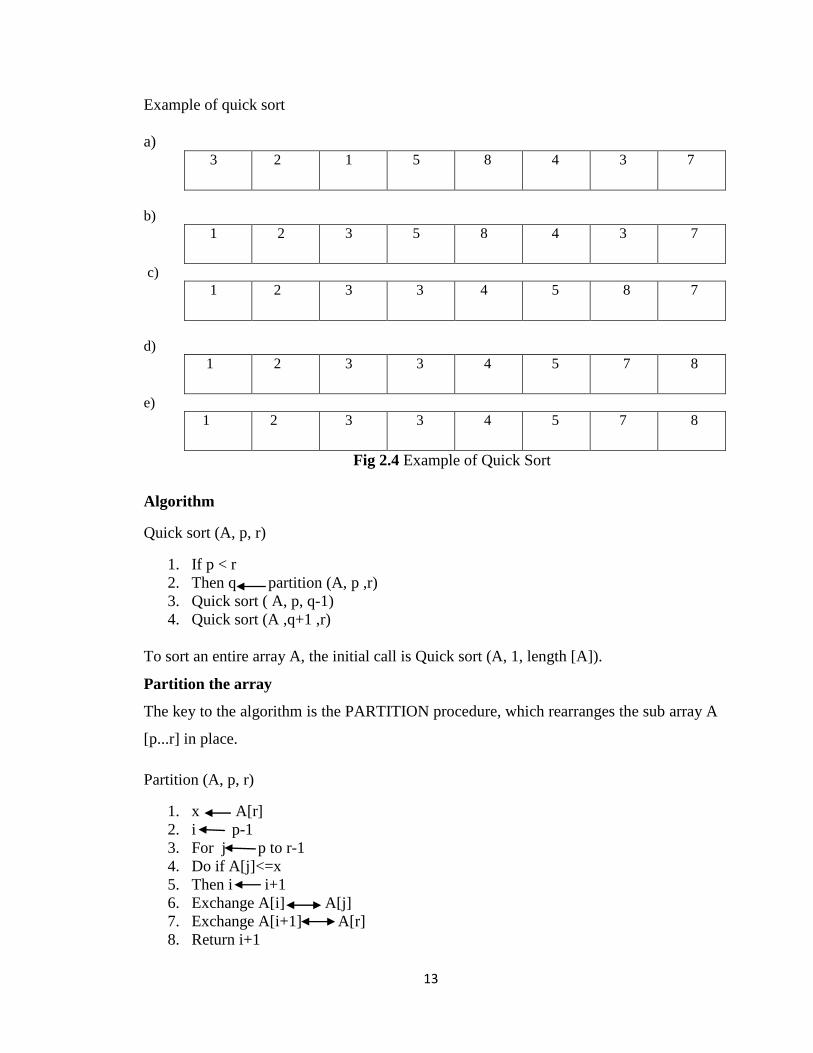
Example of quick sort

a) 3 2 1 5 8 4 3 7

b)

1 2 3 5 8 4 3 7

c)

1 2 3 3 4 5 8 7

d)

1 2 3 3 4 5 7 8

e)

1 2 3 3 4 5 7 8

Fig 2.4 Example of Quick Sort

Algorithm

Quick sort (A, p, r)

1. If p < r

2. Then q partition (A, p ,r)

3. Quick sort ( A, p, q-1)

4. Quick sort (A ,q+1 ,r)

To sort an entire array A, the initial call is Quick sort (A, 1, length [A]).

Partition the array

The key to the algorithm is the PARTITION procedure, which rearranges the sub array A

[p...r] in place.

Partition (A, p, r)

1. x A[r]

2. i p-1

3. For j p to r-1

4. Do if A[j]<=x

5. Then i i+1

6. Exchange A[i] A[j]

7. Exchange A[i+1] A[r]

8. Return i+1

14

2.6 Radix Sort

Radix sort is stable, very fast and generally is an excellent algorithm on modern

computers that usually have large memory. It is the method used by the many people

when alphabetizing a large list of names. The list of names is first sorted according to the

first letter of each name. That is; the names are arranged in 26 classes, where the first

class consists of those names that begin with “A”, the second class consists of those

names that begin with “B” and so on. Radix sort is also useful to sort records of the

information that are Keyed by multiple fields. For example we want to sort dates by three

keys: year, month and day. Radix sort is used when the size of elements are very large.

There are two approaches to radix sorting.

MSD (most-significant-digit radix sort methods): This methods examine the

digits in the keys in a left-to-right order, working with the most significant digits

first. MSD radix sorts partition the file according to the leading digits of the keys,

and then recursively apply the same method to the subfiles.

LSD (least-significant-digit radix sort methods): The second class of radix-

sorting methods examine the digits in the keys in a right-to-left order, working

with the least significant digits first.

The code of radix sort is straightforward. The following procedure assumes that each

element in the n-element array A has d digits, where digit 1 is the lower order digit and

digit d is the highest order digit.

Algorithm

Radix sort (A, d)

1. For I 1 to d

2. Do use a stable sort to sort array A on digit i

15

0 1 2 3 4 5 6 7 8 9

267 267

368 368

139

230 230

896 896

732 732

651 651

135 135

0 1 2 3 4 5 6 7 8 9

230 230

651 651

732 732

135 135

896 896

267 267

368 368

139 139

0 1 2 3 4 5 6 7 8 9

230 230

732 732

135 135

139 139

651 651

267 267

368 368

896 896

Fig 2.5 Example of Radix Sort

16

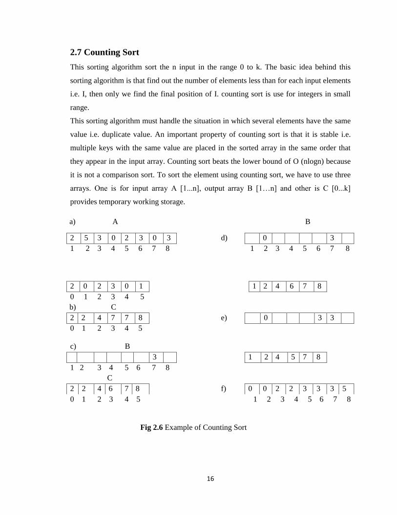
2.7 Counting Sort

This sorting algorithm sort the n input in the range 0 to k. The basic idea behind this

sorting algorithm is that find out the number of elements less than for each input elements

i.e. I, then only we find the final position of I. counting sort is use for integers in small

range.

This sorting algorithm must handle the situation in which several elements have the same

value i.e. duplicate value. An important property of counting sort is that it is stable i.e.

multiple keys with the same value are placed in the sorted array in the same order that

they appear in the input array. Counting sort beats the lower bound of O (nlogn) because

it is not a comparison sort. To sort the element using counting sort, we have to use three

arrays. One is for input array A [1...n], output array B [1…n] and other is C [0...k]

provides temporary working storage.

a) A B

0 1 2 3 4 5 1 2 3 4 5 6 7 8

Fig 2.6 Example of Counting Sort

2 5 3 0 2 3 0 3 d) 0 3

1 2 3 4 5 6 7 8

1 2 3 4 5 6 7 8

2 0 2 3 0 1 1 2 4 6 7 8

0 1 2 3 4 5

b) C

2 2 4 7 7 8 e) 0 3 3

0 1 2 3 4 5

c) B

3 1 2 4 5 7 8

1 2 3 4 5 6 7 8

C

2 2 4 6 7 8 f) 0 0 2 2 3 3 3 5

17

Algorithm

1. for I=0 to K

2. C[I]=0

3. For j=1 to length [A]

4. C [A(J)]=C[A(J)]+1

5. For I=1 to K

6. C[I]=C[I]+C[I-1]

7. For J=length(A) down to 1

8. B[C(A(J)]=A[J]

9. C[A(J)]=C[A(J)]-1

18

0.4

1.1

1.2

1.8

3.7

5.9

6.1

7.3

8.4

10.5

11.5

6.7

CHAPTER 3

SOME ADVANCED SORTING ALGORITHMS

3.1 Sorting with Address Computation (Proxmap Sort)

It is the same as counting sort. In proxmap sort with the help of an address computation

i.e. a mapping f (k) =address, a key is shifted in the first pass to the proximity of the final

destination.

Steps:

1. Definition of the mapping

2. Assignment of the neighbors

3. The interchange of the keys

4. Fine grained sorting

Example

I 0 1 2 3 4 5 6 7 8 9 10 11

A[I] 6.7 5.9 8.4 1.2 7.3 3.7 11.5 1.1 0.4 10.5 6.1 1.8

Mapping: map key (k) = └ k ┘

0 1 2 3 4 5 6 7 8 9 10 11

Fig 3.1 Example of Proxmap Sort

19

3.2 Merge Sort

Merging means combining two sorted list into one sorted list. The unsorted list is first

divide in two half. Each half is again divided into two. This is continued until we get

individual numbers. Then pairs of number are combined (merged) into sort list of two

numbers. Pairs of these lists of four numbers are merged into sorted list of eight numbers.

This is continued until the one fully sorted list is obtained.

4 2 7 8 5 1 3 6

4 2 7 8 5 1 3 6

4 2 7 8 5 1 3 6

4 2 7 8 5 1 3 6

2 4 7 8 1 5 3 6

2 4 7 8 1 3 5 6

1 2 3 4 5 6 7 8

Fig 3.2 Example of Merge Sort

20

3.3 Shell Sort

It is introduced by D.l.Shell, which uses insertion sort on periodic subsequence of the

input to produce a faster sorting algorithm. It is also known as diminishing increment

sort. It is the first sorting algorithm to break the n2 barrier. It is fast, easy to understand

and easy to implement. However, its complexity analysis is a little more sophisticated. It

begins by comparison of an element that is at a distance „d‟ which is initially half of the

no. of elements in the array. Further in each path the value of d is reduced to half i.e

di+1= (di+1)/2.

The shell sort is still significantly slower than the merge, heap, and quick sorts, but its

relatively simple algorithm makes it a good choice for sorting lists of less than 5000

items unless speed is hyper-critical. It's also an excellent choice for repetitive sorting of

smaller lists.

d=3

d=2

d=1

Fig 3.3 Example of Shell Sort

3.4 Library Sort

Library sort, or gapped insertion sort is a sorting algorithm that uses an insertion sort, but

with gaps in the array to accelerate subsequent insertions. The name comes from an

analogy: Suppose a librarian were to store his books alphabetically on a long shelf,

starting with the as at the left end, and continuing to the right along the shelf with no

spaces between the books until the end of the Zs. If the librarian acquired a new book that

belongs to the B section, once he finds the correct space in the B section, he will have to

move every book over, from the middle of the Bs all the way down to the Zs in order to

make room for the new book. This is an insertion sort. However, if he were to leave a

12 9 -10 22 2 35 40

12 2 -10 22 9 35 40

-10 2 9 22 12 35 40

-10 2 9 12 22 35 40

21

space after every letter, as long as there was still space after B, he would only have to

move a few books to make room for the new one. This is the basic principle of the

Library sort.

Library sort is a stable comparison sort and can be run as an online algorithm; however, it

was shown to have a high probability of running in O (n log n) time (comparable to quick

sort), rather than an insertion sort's O(n2). Its implementation is very similar to a skip list.

The drawback to using the library sort is that it requires extra space for its gaps (the extra

space is traded off against speed).

3.5 Heap Sort

A heap is a tree structure in which the root contains the largest (or smallest) element in

the tree. The heap sort algorithm is an improved version of the selection sort in which the

largest element (the root) is selected and exchanged with the last element in the unsorted

list. Heap sort begins by turning the array to be sorted into a heap. This is done only once

for each sort. We then exchange the root, which is the largest element in the heap, with

the last element in the unsorted list. This exchange results in the largest element being

added to the heap and exchange again. The reheap and exchange process continues until

the entire list is sorted. Creating the heap requires nlog2n loops through the data. The

heap sort efficiency is O (nlog2n). Heap sort is not a stable sort. It mainly competes with

merge sort, which has the same time bounds, but requires O (n) auxiliary space, whereas

heap sort requires only a constant amount. The heap sort is the slowest of the O (n log n)

sorting algorithms, but unlike the merge and quick sorts it doesn't require massive

recursion or multiple arrays to work. This makes it the most attractive option for very

large data sets of millions of items.

Algorithm

1. Build Max Heap (A)

2. For I length [A] downto 2

3. Do exchange A[1] A[I]

4. Heap size [A] heap size[A]-1

5. Max heapify (A,1)

22

2 4 4

4 2 2 1

4

2 1

4

3 1

2

3

5

1

2 3

3 4

4

2

1 3

2

2

3 1 2

3

1 1

5

4

Example of heap sort: 2, 4, 1, 5

(build a heap)

Now we apply heap sort

1 2 3 4 5

Fig 3.4 Example of Heap Sort

23

3.6 Gnome Sort

It is a sorting algorithm, which is similar to insertion sort, except that moving an element

to its proper place is accomplished by a series of swaps, as in bubble sort. Gnome Sort is

based on the technique used by the standard Dutch Garden Gnome. Here is how a garden

gnome sorts a line of flower pots. Basically, he looks at the flower pot next to him and

the previous one; if they are in the right order he steps one pot forward, otherwise he

swaps them and steps one pot backwards. Boundary conditions: if there is no previous

pot, he steps forwards; if there is no pot next to him, he is done. It is conceptually simple,

requiring no nested loops. The running time is O(n²), but in practice the algorithm can run

as fast as Insertion sort. The algorithm always finds the first place where two adjacent

elements are in the wrong order, and swaps them. It takes advantage of the fact that

performing a swap can introduce a new out-of-order adjacent pair only right before or

after the two swapped elements. It does not assume that elements forward of the current

position are sorted, so it only needs to check the position directly before the swapped

elements.

If we wanted to sort an array with elements [4] [2] [7] [3], here is what would happen

with each of the iteration of the while loop

[4] [2] [7] [3] (initial state. i is 1 and j is 2)

[4] [2] [7] [3] (did nothing, but now i is 2 and j is 3.)

[4] [7] [2] [3] (swapped a[2] and a[1]. now i is 1 and j is still 3.)

[7] [4] [2] [3] (swapped a[1] and a[0]. now i is 1 and j is still 3.)

[7] [4] [2] [3] (did nothing, but now i is 3 and j is 4.)

[7] [4] [3] [2] (swapped a[3] and a[2]. now i is 2 and j is 4.)

[7] [4] [3] [2] (did nothing, but now i is 4 and j is 5.)

At this point the loop ends because it isn't equal to 4.

3.7 Stack Sort

This algorithm is called Stack Sort here as it uses the data structure stack in both the

distribution and collection phases, which are described below.

24

The group of stacks is managed by maintaining an ordered linked list of pointers to the

stacks. The individual stacks are also maintained as linked lists. Arrays are unsuitable for

the stacks and also for the pointers to them as the size of the individual stacks and the

pointers list can vary widely between 1 and N, where N is the size of the input.

The algorithm is sensitive to the order already existing in the input:

The best case occurs when the input is already in increasing order, because only

one sublist holding all the N items would be formed.

The worst case occurs when the input is already sorted in reverse order, because

there will be N sublists, each containing only one item.

The algorithm involves only comparisons between items and no data exchanges. The

algorithm selects maximum items like HeapSort. The maximum item is the tail item of

the first sublist. There is little work involved in the maintenance of the sublists in the

required order. However, on the negative side, there is the overhead of maintaining

pointers for the linked lists and extra space requirement.

3.7.1 The distribution phase of Stack Sort

The distribution phase uses the algorithm described by Moffat and Petersson [Moffat,

1992].

In this phase the input list is distributed into sublists in such a way that

Each sublist contains an ascending subsequence from head to tail, the tail item

is greater than or equal to every other item in the sublist.

The sublists are also ordered so that their tail items are in descending order. The

tail item of the first sublist is greater than the tail item of the second sublist,

which is greater than the tail item of the next sublist and so on.

For example, consider the following input list.

(9, 5, 6, 3, 8, 7, 1, 11, 2, 10, 5, 12)

sublist1 9 11 12

sublist2 5 6 8 10

sublist3 3 7

sublist4 1 2 5

Note that at the end of the distribution phase:

25

The items in each sublist are in increasing order from head to tail constituting one

'run', but the items are not adjacent in the input.

The tail items of the sublists are in descending order. The tail item of sublist1 is

the largest item in the input list.

The number of sublists, 4, is less than the number of runs, 7, in the original data.

3.7.2 The collection phase of Stack Sort

The tail item of sublist1, the maximum item, is deleted from that list and written to the

output list. The sublists are rearranged, if necessary, such that the tail items continue to be

in descending order. The tail item of sublist1 continues to supply the next maximum to be

written to the output list. The process continues until all items are written to the output

list.

Since all the actions on each sublist take place on its tail item, the stack structure is ideal

for the sublist implementation. The output list also collects the items in reverse,

descending, order. The output list may also be implemented as a stack.

Working of the collection phase may be illustrated using the sublists above. The sublists

are now designated as stacks S1, S2, etc. The following stacks were formed at the end of

the distribution phase:

S1 9 11 12

S2 5 6 8 10

S3 3 7

S4 1 2 5

(Stacks are shown growing to the right; the right most element is at the top)

Start by popping 12 from S1 and pushing it on to the output stack. This is followed by

popping 11 from S1 and pushing it on to output stack. Now the stack S1 has its tail item,

9, less than the tail item of the second stack. Hence the stacks are reordered as follows to

maintain the tail items in descending order.

S2 5 6 8 10

S1 9

S3 3 7

S4 1 2 5

Now 10 is popped from the first stack S2, and the stacks reordered:

26

S1 9

S2 5 6 8

S3 3 7

S4 1 2 5

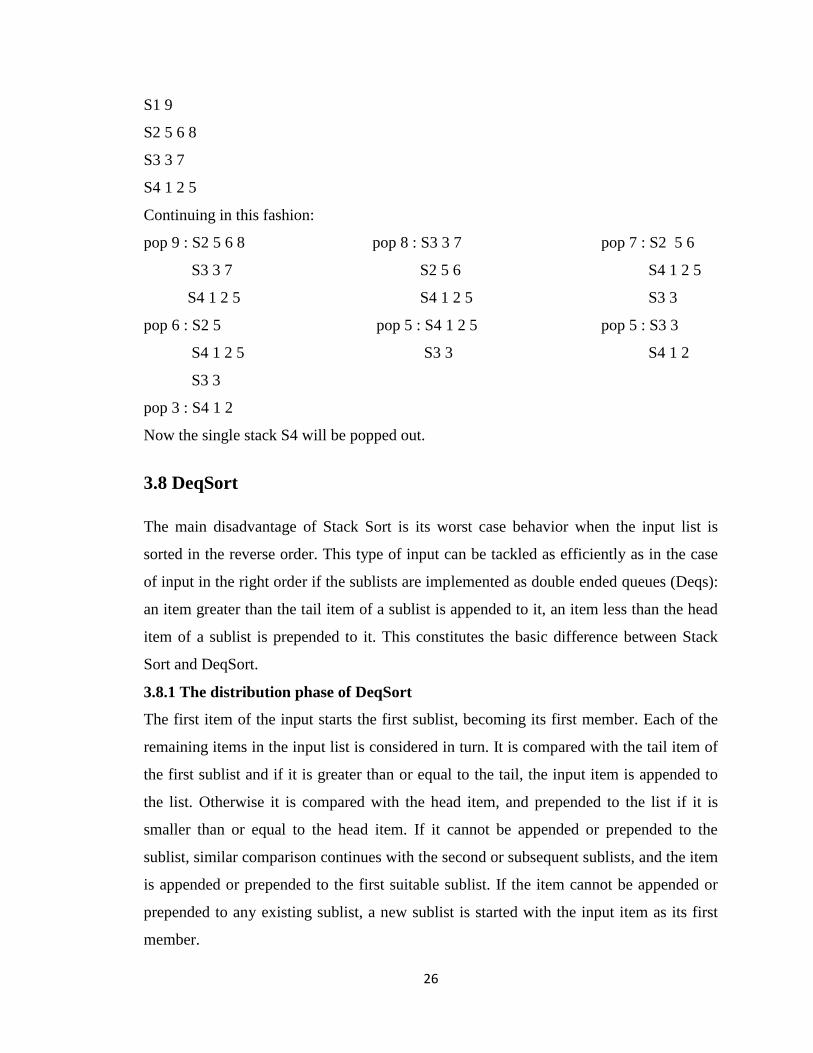
Continuing in this fashion:

pop 9 : S2 5 6 8 pop 8 : S3 3 7 pop 7 : S2 5 6

S3 3 7 S2 5 6 S4 1 2 5

S4 1 2 5 S4 1 2 5 S3 3

pop 6 : S2 5 pop 5 : S4 1 2 5 pop 5 : S3 3

S4 1 2 5 S3 3 S4 1 2

S3 3

pop 3 : S4 1 2

Now the single stack S4 will be popped out.

3.8 DeqSort

The main disadvantage of Stack Sort is its worst case behavior when the input list is

sorted in the reverse order. This type of input can be tackled as efficiently as in the case

of input in the right order if the sublists are implemented as double ended queues (Deqs):

an item greater than the tail item of a sublist is appended to it, an item less than the head

item of a sublist is prepended to it. This constitutes the basic difference between Stack

Sort and DeqSort.

3.8.1 The distribution phase of DeqSort

The first item of the input starts the first sublist, becoming its first member. Each of the

remaining items in the input list is considered in turn. It is compared with the tail item of

the first sublist and if it is greater than or equal to the tail, the input item is appended to

the list. Otherwise it is compared with the head item, and prepended to the list if it is

smaller than or equal to the head item. If it cannot be appended or prepended to the

sublist, similar comparison continues with the second or subsequent sublists, and the item

is appended or prepended to the first suitable sublist. If the item cannot be appended or

prepended to any existing sublist, a new sublist is started with the input item as its first

member.

27

Each sublist holds one subsequence in ascending order from head to tail. The tail item in

each sublist is the largest in that sublist. The sublists themselves are also ordered such

that their respective tail items are in descending order. In addition, the head items are in

ascending order.

For example, consider the same input list which was used to illustrate the StackSort in

Section 3.7.1.

(9, 5, 6, 3, 8, 7, 1, 11, 2, 10, 5, 12)

The sublists SL1, SL2,...will be built as follows.

read 9 : SL1 9 read 5 : SL1 5 9 read 6 :SL1 5 9

SL2 6

read 3 : SL1 3 5 9 read 8 : SL1 3 5 9 read 7 : SL1 3 5 9

SL2 6 SL2 6 8 SL2 6 8

SL3 7

..... and so on.

At the end this phase the following sublists will be produced:

SL1 1 3 5 9 11 12

SL2 2 6 8 10

SL3 5 7

Note that

The number of sublists, 3, is smaller than the number of runs, 7; and also smaller

than the number of sublists produced by StackSort.

The head items are in ascending order.

3.8.2 The collection phase of DeqSort

In the collection phase one can extract either the head items (current minimum) or the tail

items (current maximum) from the first sublist. The description below is for the option of

extracting head items. The extraction of head items results in writing to output in

ascending order. Once an item is extracted, it will not be simple to reorder the sublists so

as to maintain both the head and the tail items in the required order. Thus only the head

items will be maintained in ascending order.

28

Working of the collection phase may be illustrated using the following sublists which

were formed at the end of the distribution phase:

SL1 1 3 5 9 11 12

SL2 2 6 8 10

SL3 5 7

Start by dequeueing 1 from SL1 and writing it to the output list. Since the new head of

SL1 (3) is greater than head of SL2, reorder the lists:

SL2 2 6 8 10

SL1 3 5 9 11 12

SL3 5 7

Dequeue 2, append it to output list, reorder the lists:

SL1 3 5 9 11 12

SL3 5 7

SL2 6 8 10

Continuing in this fashion:

Deque 3 : SL1 5 9 11 12 Deque 5 : SL3 5 7

SL3 5 7 SL2 6 8 10

SL2 6 8 10 SL1 9 1 12

Deque 5 : SL2 6 8 10 Deque 6 : SL3 7 Deque 7 :SL2 8 10

SL3 7 SL2 8 10 SL1 9 11 12

SL1 9 1 12 SL1 9 11 12

Deque 8 : SL1 9 1 12 Deque 9 : SL2 10 Deque 10 : SL1 11 12

SL2 10 SL1 11 12 SL1 can be written out.

3.9 MinMax Sort

At the end of the distribution phase of DeqSort (Section 3), the sublists are ordered in

such a way that the head items are in ascending order and the tail items are in descending

order. The collection phase however maintains only the head items in ascending order

while extracting the minimum items. MinMaxSort is a variation of DeqSort in which both

29

the minimum and the maximum items are extracted at the same time. This would require

that the sublists maintain both the head and the tail items in the required order.

3.9.1 The distribution phase of MinMaxSort

This is identical to the distribution phase of DeqSort and is already described in Section

3.8.1.

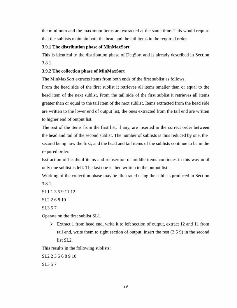
3.9.2 The collection phase of MinMaxSort

The MinMaxSort extracts items from both ends of the first sublist as follows.

From the head side of the first sublist it retrieves all items smaller than or equal to the

head item of the next sublist. From the tail side of the first sublist it retrieves all items

greater than or equal to the tail item of the next sublist. Items extracted from the head side

are written to the lower end of output list, the ones extracted from the tail end are written

to higher end of output list.

The rest of the items from the first list, if any, are inserted in the correct order between

the head and tail of the second sublist. The number of sublists is thus reduced by one, the

second being now the first, and the head and tail items of the sublists continue to be in the

required order.

Extraction of head/tail items and reinsertion of middle items continues in this way until

only one sublist is left. The last one is then written to the output list.

Working of the collection phase may be illustrated using the sublists produced in Section

3.8.1.

SL1 1 3 5 9 11 12

SL2 2 6 8 10

SL3 5 7

Operate on the first sublist SL1.

Extract 1 from head end, write it to left section of output, extract 12 and 11 from

tail end, write them to right section of output, insert the rest (3 5 9) in the second

list SL2.

This results in the following sublists:

SL2 2 3 5 6 8 9 10

SL3 5 7

30

Operate on SL2.

Extract 2, 3, 5 from head end, write to left section of output, and extract 10, 9, 8

from tail end, write to right section of output, insert the rest (6) in SL3.

Now a single sublist is left. SL3 5 6 7.

SL3 is written to the output list.

MinMaxSort, similar to DeqSort, handles input ordered in any way almost equally well.

The best case occurs when input is already sorted, whether right or reverse order does not

matter.

To facilitate the append/prepend operations in the distribution phase and also the

extraction of the head and tail items in the collection phase, the sublists are best

maintained as doubly linked lists.

MinMaxSort has the potential to reduce the number of sublists significantly. However, it

is more complicated than DeqSort and has higher storage overhead as the sublists are

doublylinked.

3.10 New sorting algorithm [21,22]

It is a new sorting algorithm introduced by kiran kumar sundararajan and Soubhik

chakraborty. This sorting algorithm works on the “divide and conquer strategy” similar to

quick sort but the use of auxiliary array results in avoiding interchanges of elements,

thereby sacrificing space. This sorting algorithm work well for n<=1,5,00,000 as

comparison to heap sort. However it slows down for higher n.

Step 1: Initialize the first element of the array as a pivot (key) element.

Step 2: Starting from the second element, compare it to the pivot element.

Step 2.1: if pivot < element then place the element in the last unfilled position of a

temporary array (of same size as the original one).

Step 2.2: if pivot > element then place the element in the first unfilled position of the

temporary array.

Step 3: repeat step 2 till last element of the array.

31

Step 4: finally place the pivot element in the blank position of the temporary array (the

blank position is created because one element of the original array was taken out as pivot)

Step 5: split the array into two, based on the pivot element's position.

Pseudo Code

My_sort (int numbers[], int b[],int l, int r)

{

// pivot=first element of array, low=l, up=r ,numbers[] is the Original array, b[] is temp

array.

//l is left index and r is right index

// My logic starts here.

for (i=l+1; i<=r; i++)

{

if (numbers[i] <= pivot)

{

b[low] = numbers[i];

low++;

}

else

{

b[up]=numbers[i];

up--;

}

}

b[low]=pivot;

for (i = l; i <= r; i++)

numbers[i]=b[i];

if (l < up-1)

My_sort(b,numbers, l, up-1);

if(up+1 < r)

My_sort(b,numbers, up+1,r);

}

32

CHAPTER4

SORTING NETWORK

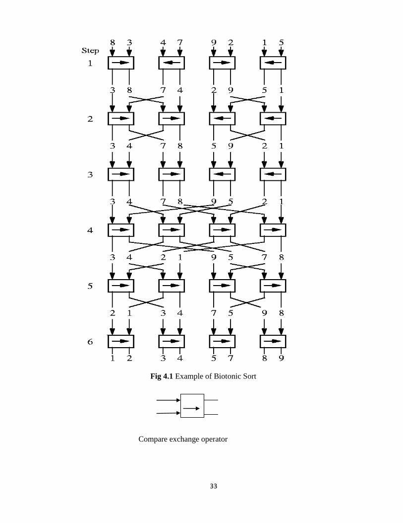
4.1Bitonic Sort

It is a kind of sorting network which sort n elements in O(log2

n) Time. The operation of

the bitonic sorting network is the rearrangement of a bitonic sequence into a sorted list.

Biotonic sequence

A bitonic sequence is a sequence of the elements(a0,a1,…………an-1) with the two

property that either 1 ) there exits an index i , 0<=i<=n-1,such that (a0,a1,……………,ai)

is monotonically increasing and (ai+1,…………an-1) is monotonically decreasing .or

2) There is a cyclic shift of indices so that (1) is satisfied.

Examples are {1,4,6,8,3,2},{6,9,4,2,3,5},{9,8,3,2,4,6}.

We have a method for merging a bitonic sequence into a sorted sequence. This method is

easy to implement on a network of comparators.This network of comparators, known as

bitonic merging network. Following are the example of merging a 16 element biotonic

sequence through a series of log16 bitonic splits.

Original

Sequence 3 5 8 9 10 12 14 20 95 90 60 40 35 23 18 0

1st split 3 5 8 9 10 12 14 0 95 90 60 40 35 23 18 95

2nd split 3 5 8 0 10 12 14 9 35 23 18 20 95 90 60 40

3rd split 3 0 8 5 10 9 14 12 18 20 35 23 60 40 95 90

4th split 0 3 5 8 9 10 12 14 18 20 23 35 40 60 90 95

33

Fig 4.1 Example of Biotonic Sort

Compare exchange operator

34

4.2 Odd-even Sorting Network

The odd-even transposition algorithm sorts n elements in n phase where n is even. This

algorithm alternate between two phases called the odd and even phases. Let

(a1,a2……..,an) be the sequence to be sorted. During the odd phase, elements with odd

indices are compared with their right neighbors and if they are out of sequence they are

exchanged i.e. the pair (a1,a2),(a3,a4)…………(an-1,an) are compare-exchanged where n is

even. And during even phase, pairs (a2,a3),(a4,a5),………..(an-2,an-1) are compare-

exchanged.

Algorithm

1. Begin

2. For I=1 to n do

3. Begin

4. If I is odd then

5. For j=0 to n/2-1 do

6. Compare-exchange(a2j+1 ,a2j+2)

7. If n is even then

8. For j=1 to n/2-1 do

9. Compare-exchange(a2j,a2j+1)

10. End for.

Example

3 2 3 8 5 6 4 1

Phase 1(odd) 2 3 3 8 5 6 1 4

Phase 2(even) 2 3 3 5 8 1 6 4

Phase 3(odd ) 2 3 3 5 1 8 4 6

Phase 4 (even) 2 3 3 1 5 4 8 6

Phase 5(odd) 2 3 1 3 4 5 6 8

Phase 6(even) 2 1 3 3 4 5 6 8

Phase 7(odd) 1 2 3 3 4 5 6 8

Phase 8(even) 1 2 3 3 4 5 6 8

35

CHAPTER 5

PROBLEM STATEMENT

The problem of sorting is a problem that arises frequently in computer programming.

Many different sorting algorithms have been developed and improved to make sorting

fast. As a measure of performance mainly the average number of operations or the

average execution times of these algorithms have been investigated and compared.

5.1 Problem statement

All sorting algorithms are nearly problem specific. How one can predict a suitable sorting

algorithm for a particular problem? What makes good sorting algorithms? Speed is

probably the top consideration, but other factors of interest include versatility in handling

various data types, consistency of performance, memory requirements, length and

complexity of code, and stability factor (preserving the original order of records that have

equal keys).

For example, sorting a database which is so big that cannot fit into memory all at once is

quite different from sorting an array of 100 integers. Not only will the implementation of

the algorithm be quite different, naturally, but it may even be that the same algorithm

which is fast in one case is slow in the other. Also sorting an array may be different from

sorting a linked list.

5.2 Justification

In order to judge suitability of a sorting algorithm to a particular problem we need to see

Are the data that application needs to sort tending to have some pre existing

order?

What are properties of data being sorted?

Do we need a stable sort?

36

Can you use some "extra" memory or need "in-place" soft? (with the current

computer memory sizes we usually can afford some additional memory so

"in-place" algorithms no longer have any advantages).

Generally the more we know about the properties of data to be sorted, the faster we can

sort them. As we already mentioned the size of key space is one of the most important

factors (sort algorithms that use the size of key space can sort any sequence for time O (n

log k).

5.3 Explanation

Many different sorting algorithms have been invented so far. Why are there so many

sorting methods? For computer science, this is a special case of question, “why there are

so many x methods?”, where x ranges over the set of problem; and the answer is that each

method has its own advantages and disadvantages, so that it outperforms the others on the

same configurations of data and hardware. Unfortunately, there is no known “best” way

to sort; there are many best methods, depending on what is to be sorted on what machine

and for what purpose. There are many fundamental and advance sorting algorithms. All

sorting algorithm are problem specific means they work well on some specific problem,

not all the problems. All sorting algorithm apply to specific kind of problems. Some

sorting algorithm apply to small number of elements, some sorting algorithm suitable for

floating point numbers, some are fit for specific range like (0 1].some sorting algorithm

are used for large number of data, some are used for data with duplicate values.

It is not always possible to say that one algorithm is better than another, as relative

performance can vary depending on the type of data being sorted. In some situations,

most of the data are in the correct order, with only a few items needing to be sorted; In

other situations the data are completely mixed up in a random order and in others the data

will tend to be in reverse order. Different algorithms will perform differently according to

the data being sorted.

37

CHAPTER 6

RESULT AND DISCUSSION

6.1 Problem Definition and Sorting Algorithms

All the sorting algorithms are problem specific. Each sorting algorithms work well on

specific kind of problems. In this table we described some problems and analyses that

which sorting algorithm is more suitable for that problem.

Table 6.1: problem definition and sorting algorithms

Problem Definition Sorting Algorithms

The data to be sorted is small enough to fit into a processor‟s

main memory and can be randomly accessed i.e. no extra space

is required to sort the records (Internal Sorting).

Insertion Sort,

Selection Sort, Bubble

Sort

Source data and final result are both sorted in hard disks (too

large to fit into main memory), data is brought into memory for

processing a portion at a time and can be accessed sequentially

only (External Sorting).

Merge Sort (business

application, database

application)

The input elements are uniformly distributed within the range

[0, 1).

Bucket Sort

Constant alphabet (ordered alphabet of constant size, multi set

of characters can be stored in linear time), sort records that are

of multiple fields.

Radix Sort

The input elements are small.

Insertion Sort

The input elements are too large. Merge Sort, Shell Sort,

Quick Sort, Heap Sort

The data available in the input list are repeated more times i.e.

occurring of one value more times in the list.

Counting Sort

The input elements are sorted according to address (Address

Computation).

Proxmap Sort, Bucket

Sort

38

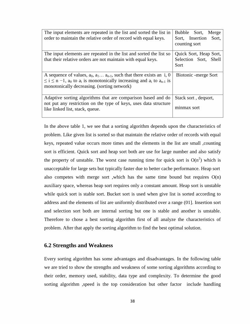
The input elements are repeated in the list and sorted the list in

order to maintain the relative order of record with equal keys.

Bubble Sort, Merge

Sort, Insertion Sort,

counting sort

The input elements are repeated in the list and sorted the list so

that their relative orders are not maintain with equal keys.

Quick Sort, Heap Sort,

Selection Sort, Shell

Sort

A sequence of values, a0, a1… an-1, such that there exists an i, 0

≤ i ≤ n −1, a0 to ai is monotonically increasing and ai to an-1 is

monotonically decreasing. (sorting network)

Biotonic -merge Sort

Adaptive sorting algorithms that are comparison based and do

not put any restriction on the type of keys, uses data structure

like linked list, stack, queue.

Stack sort , deqsort,

minmax sort

In the above table 1, we see that a sorting algorithm depends upon the characteristics of

problem. Like given list is sorted so that maintain the relative order of records with equal

keys, repeated value occurs more times and the elements in the list are small ,counting

sort is efficient. Quick sort and heap sort both are use for large number and also satisfy

the property of unstable. The worst case running time for quick sort is O(n2) which is

unacceptable for large sets but typically faster due to better cache performance. Heap sort

also competes with merge sort ,which has the same time bound but requires O(n)

auxiliary space, whereas heap sort requires only a constant amount. Heap sort is unstable

while quick sort is stable sort. Bucket sort is used when give list is sorted according to

address and the elements of list are uniformly distributed over a range (01]. Insertion sort

and selection sort both are internal sorting but one is stable and another is unstable.

Therefore to chose a best sorting algorithm first of all analyze the characteristics of

problem. After that apply the sorting algorithm to find the best optimal solution.

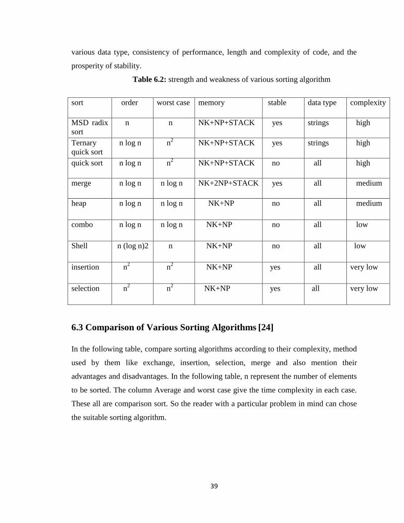
6.2 Strengths and Weakness

Every sorting algorithm has some advantages and disadvantages. In the following table

we are tried to show the strengths and weakness of some sorting algorithms according to

their order, memory used, stability, data type and complexity. To determine the good

sorting algorithm ,speed is the top consideration but other factor include handling

39

various data type, consistency of performance, length and complexity of code, and the

prosperity of stability.

Table 6.2: strength and weakness of various sorting algorithm

sort order worst case memory stable data type complexity

MSD radix

sort

n n NK+NP+STACK yes strings high

Ternary

quick sort

n log n

n2 NK+NP+STACK yes strings high

quick sort n log n

n2 NK+NP+STACK no all high

merge n log n

n log n

NK+2NP+STACK yes all medium

heap n log n

n log n

NK+NP no all medium

combo n log n

n log n

NK+NP no all low

Shell

n (log n)2

n NK+NP no all low

insertion n2 n

2 NK+NP yes all very low

selection n2 n

2 NK+NP yes all very low

6.3 Comparison of Various Sorting Algorithms [24]

In the following table, compare sorting algorithms according to their complexity, method

used by them like exchange, insertion, selection, merge and also mention their

advantages and disadvantages. In the following table, n represent the number of elements

to be sorted. The column Average and worst case give the time complexity in each case.

These all are comparison sort. So the reader with a particular problem in mind can chose

the suitable sorting algorithm.

40

6.3.1 Comparison of Comparison Based Sorting Algorithms

Table 6.3: Comparison of Comparison Based Sort

Name Average Case Worst

Case

Method Advantage/Disadvantage

Bubble Sort O(n2) O(n

2) Exchange 1. Straightforward, simple and

slow.

2. Stable.

3. Inefficient on large tables.

Insertion

Sort

O(n2) O(n

2) Insertion 1. Efficient for small list and

mostly sorted list.

2. Sort big array slowly.

3. Save memory

Selection

Sort

O(n2) O(n

2) Selection 1. Improves the performance of

bubble sort and also slow.

2. Unstable but can be

implemented as a stable sort.

3. Quite slow for large amount of

data.

Heap Sort O(n log n) O(n log n) Selection 1. More efficient version of

selection sort.

2. No need extra buffer.

3. Its does not require recursion.

4. Slower than Quick and Merge

sorts.

Merge Sort O(n log n) O(n log n) Merge 1. Well for very large list, stable

sort.

2. A fast recursive sorting.

3. Both useful for internal and

external sorting.

4. It requires an auxiliary array

that is as large as the original array

to be sorted.

In place-

merge Sort

O(n log n) O(n log n) Merge 1. Unstable sort.

2. Slower than heap sort.

3. Needs only a constant amount

of extra space in addition to that

needed to store keys.

41

Shell Sort O(n log n) O(nlog2n) Insertion 1. Efficient for large list.

2. It requires relative small amount

of memory, extension of insertion

sort.

3. Fastest algorithm for small list

of elements.

4. More constraints, not stable.

Cocktail

Sort

O(n2) O(n

2) Exchange 1. Stable sort.

2. Variation of bubble sort.

3. Bidirectional bubble sort.

Quick Sort O(n log n) O(n2) Partition 1. Fastest sorting algorithm in

practice but sometime Unbalanced

partition can lead to very slow

sort.

2. Available in many slandered

libraries.

3. O (log n) space usage.

4. Unstable sort and complex for

choosing a good pivot element.

Library sort O(n log n) O(n2) Insertion 1.Stable

2. It requires extra space for its

gaps.

Gnome sort O(n2) O(n

2) Exchange 1.Stable

2. Tiny code size.

3. similar to insertion sort.

6.3.2 Comparison of Non Comparison Based Sorting Algorithms

The following table described sorting algorithm which are not comparison sort.

Complexities below are in terms of n, the number of item to be sorted, k the size of each

key and s is the chunk size use by implementation. Some of them are based on the

assumption that the key size is large enough that all entries have unique key values, and

hence that n << 2k.

42

Table 6.4: Comparison of Non -Comparison Sort

Name Average

Case

Worst Case n<<2K Advantage/disadvantage

Bucket Sort O(n.k) O(n2.k) No 1. Stable, fast.

2. Valid only in range o to

some maximum value M.

3. Used in special cases when

the key can be used to

calculate the address of

buckets.

Counting Sort O(n+2k) O(n+2

k) Yes 1. Stable, used for repeated

value.

2. Often used as a subroutine

in radix sort.

3. Valid in the rang(o k]

Where k is some integer.

Radix Sort O(n.

k

s)

O(n.k

s)

No 1. Stable, straight forward

code.

2. Used by the card-sorting

machines.

3. Used to sort records that

are keyed by multiple fields

like date (Year, month and

day).

MSD Radix

Sort O(n.

k

s)

O(n.k

s)

No 1. Enhance the radix sorting

methods, unstable sorting.

2. To sort large computer

files very efficiently without

the risk of overflowing

allocated storage space.

3. Bad worst-case

performance due to

fragmentation of the data into

many small sub lists.

4. It inspects only the

significant characters.

LSD Radix

Sort O(n.

k

s)

O(n.k

s. 2s)

No 1. It inspects a complete

horizontal strip at a time.

2. It inspects all characters of

the input.

3. Stable sorting method.

43

CHAPTER 7

CONCLUSION

In this thesis, we have study about various sorting algorithms. Therefore, to sort a list of

elements, First of all we analyzed the given problem i.e. the given problem is of which

type (small numbers, large values). After that we apply the sorting algorithms but keep in

mind minimum complexity, minimum comparison and maximum speed. In this thesis we

also discuss the advantages and disadvantages of sorting techniques to choose the best

sorting algorithms for a given problem. Finally, the reader with a particular problem in

mind can choose the best sorting algorithm.

From time to time people ask the ageless question: Which sorting algorithm is the better?

This question doesn't have an easy or unambiguous answer, however. The speed of

sorting can depend quite heavily on the environment where the sorting is done, the type

of items that are sorted and the distribution of these items.

There are two major factors when measuring the performance of a sorting algorithm. The

algorithms have to compare the magnitude of different elements and they have to move

the different elements around. So counting the number of comparisons and the number of

exchanges or moves made by an algorithm offer useful performance measures. When

sorting large record structures, the number of exchanges made may be the principal

performance criterion, since exchanging two records will involve a lot of work. When

sorting a simple array of integers, then the number of comparisons will be more

important.

Sorting algorithms work well on specific type of problem. Some sorting algorithms

maintain the relative order of record with equal keys like bubble sort, merge sort,

counting sort, insertion sort. Quick sort, heap sort, selection sort, shell sort sorted the

input list so that the relative order are not maintain with equal keys. When no extra space

is required to sort the record we use insertion sort, selection sort, bubble sort (internal

sorting). Merge sort (external sorting) is used in business application, database

application. Bucket sort is used when the data to be sorted are uniformly distributed

44

within the range (0 1]. Insertion sort is used for small number of element while merge

sort, quick sort, heap sort are used for large list. Counting sort is used when the data

available in the input list are repeated more number of times. The input lists are sorted

according to address (address computation) proxmap sort and bucket sort are used.

The selection sort is a good one to use. It is intuitive and very simple to program. It

offers quite good performance, its particular strength being the small number of

exchanges needed. For a given number of data items, the selection sort always goes

through a set number of comparisons and exchanges, so its performance is predictable.

Among non-stable algorithms Shell sort is probably the most underappreciated and quick

sort is one of the most overhyped. Quick sort is a fragile algorithm because the choice of

pivot is equal to guessing an important property of the data to be sorted (and if it went

wrong the performance can be close to quadratic). Without enhancements it does not

work well on "almost sorted" data (for example sorted in reverse order) and that is an

important in real world deficiency.

Shell sort and heap sort don't show too much of a difference, even though the former

might be slightly slower in average with very big arrays. Almost sorted arrays seem to be

faster for both to sort.

The common sorting algorithms can be divided into two classes by the complexity of

their algorithms. The two classes of sorting algorithms are O(n2), which includes the

bubble, insertion, selection, and shell sorts; and O(n log n) which includes the heap,

merge, and quick sorts. Quick sort is efficient only on the average, and its worst case is

n2, while heap sort has an interesting property that the worst case is not much different

from an average case.

In addition to algorithmic complexity, the speed of the various sorts can be compared

with empirical data. Since the speed of a sort can vary greatly depending on what data set

it sorts, accurate empirical results require several runs of the sort be made and the results

averaged together.

45

Some examples of sorting algorithms based on the two phase paradigm are Merge Sort,

Natural Merge Sort, Radix Sort [Aho, 1974], [Kingston, 1990].

The Stack Sort, DeqSort and MinMax Sort algorithms are based only on comparison of

input data elements. They involve no data exchanges, which are required in most other

algorithms such as Insertion Sort, Selection Sort, Heap Sort and Quick Sort. When the

size of the elements to be sorted is large, absence of data exchanges is an advantage.

Most internal sorting algorithms need the input data to be read into an array for sorting.

Stack Sort, DeqSort and MinMax Sort do not need to do this. The data read from an input

file can be inserted straight into an appropriate sublist in the distribution phase.

After analyzing the different sorting algorithm for particular problems, we conclude that,

based on the problem characteristics different algorithms are efficient for different

problems. We can‟t say particular sorting algorithm is efficient for all kind of problems.

Based on problem criteria and characteristics one of the sorting algorithm is efficient.

Like this for different problems different sorting algorithms are suitable to find best

optimal solution.

46

ANNEXURE-I

REFERENCES

[1] Knuth, D.”The Art of Computer programming Sorting and Searching”, 2nd

edition, vol.3. Addison- Wesley, 1998.

[2] Wirth, N., 1976. “Algorithms + Data Structures = Programs”: Prentice-Hall, Inc.

Englewood Cliffs, N.J.K. Mehlhorn. Sorting and Searching. Springer Verlag,

Berlin, 1984.

[3] LaMarca and R. Ladner.” The Influence of Caches on the Performance of

Sorting.” In Proceeding of the ACM/SIAM Symposium on Discrete Algorithms,

pages 370–379, January 1997.

[4] Hoare, C.A.R. “Algorithm 64: Quick sort”. Comm. ACM 4, 7 (July 1961), 321.

[5] G. Franceschini and V. Geffert. “An In-Place Sorting with O (n log n)

Comparisons and O (n) Moves”. In Proc. 44th Annual IEEE Symposium on

Foundations of Computer Science, pages 242–250, 2003.

[6] D. Jim´enez-Gonz´alez, J. Navarro, and J. Larriba-Pey. CC-Radix: “A Cache

Conscious Sorting Based on Radix Sort”. In Euromicro Conference on Parallel

Distributed and Network based Processing, pages 101–108, February 2003.

[7] J. L. Bentley and R. Sedgewick. “Fast Algorithms for Sorting and Searching

Strings”, ACM-SIAM SODA ‟97, 360–369, 1997.

[8] Flores, I. “Analysis of Internal Computer Sorting”. J.ACM 7, 4 (Oct. 1960), 389-

409.

[9] Flores, I.”Analysis of Internal Computer Sorting”. J.ACM 8, (Jan. 1961), 41-80.

[10] ANDERSSON, A. and NILSSON, S. 1994. “A New Efficient Radix Sort”. In

Proceeding of the 35th

Annual IEEE Symposium on Foundation of Computer

Science (1994),pp. 714-721.

[11] DAVIS, I.J. 1992. “A Fast Radix Sort”. The computer journal 35, 6, 636-642.

[12] V.Estivill-Castro and D.Wood.“A Survey of Adaptive Sorting Algorithms”,

Computing Surveys, 24:441–476, 1992.

47

[13] T. H. Cormen, C. E. Leiserson, R. L. Rivest, and C. Stein.”Introduction to

Algorithms”. MIT Press, Cambridge, MA, 2nd edition, 2001.

[14] D. Jim´enez-Gonz´alez, J. Navarro, and J. Larriba-Pey. CC-Radix: “A Cache

Conscious Sorting Based on Radix Sort”. In Euromicro Conference on Parallel

Distributed and Network based Processing, pages101–108, February 2003.

[15] A.Aggarwal and J. S. Vitter.”The Input/Output Complexity of Sorting And

Related Problems”. Communications of the ACM, 31(9):1116–1127, 1988.

[16] R. W. Floyd. “Algorithm 245: Treesort3”. Communications of the ACM,

7(12):701, 1964.

[17] Aho, A.V., Hopcroft, J.E., Ullman, J. D., 1974.”The Design and Analysis of

Computer Algorithms” Addison-Wesley.

[18] MacLaren, M.D. “Internal Sorting By Radix Plus Sifting”. J. ACM 13, 3 (July

1966), 404-- 411.

[19] Williams, J.W.J. “Algorithm 232: Heap sort”. Comm. ACM 7, 6 (June 1964),

347-348.

[20] J. Larriba-Pey, D. Jim´enez-Gonz´alez,and J. Navarro. “An Analysis of

Superscalar Sorting Algorithms on an R8000 processor”. In International

Conference of the Chilean Computer Science Society pages 125–134, November

1997.

[21] A. Aho, J. Hopcroft, J. Ullman, “Data Structures and Algorithms”, Pearson India

reprint, 2000

[22] R. Motwani and P. Raghavan, “Randomized Algorithms”,Cambridge University

Press, 2000

[23] Aditya Dev Mishra, Deepak Garg “Selection of Best Sorting Algorithm”

International Journal of Intelligent Information Processing” Vol II Issue II 2008

ISSN0.973-3892, p. 233-238.

[24] Y. Han “Deterministic Sorting In O(nlog Log n) Time And Linear Space”,

Proceedings of the thirty-fourth annual ACM symposium on Theory of

computing, Montreal, Quebec, Canada, 2002, p.602-608.

48

[25] M. Thorup ,“Randomized Sorting in O (n log log n) Time and Linear Space Using

Addition, Shift, and Bit-wise Boolean Operations”, Journal of Algorithms,

Volume 42, Number 2, February 2002, p. 205-230.

[26] Y. Han, M. Thorup, “Integer Sorting in O(n √(log log n) Time and Linear Space”,

Proceedings of the 43rd Symposium on Foundations of Computer Science, 2002,

p. 135-144.

[27] P. M. McIlroy, K. Bostic and M. D. McIlroy, “Engineering Radix Sort”,

Computing Systems, 2004, p.224-230.

49

ANNEXURE II

LIST OF PUBLICATIONS

[1] Aditya Dev Mishra, Deepak Garg “Selection of Best Sorting Algorithm”

International Journal of Intelligent Information Processing” Vol II Issue II 2008

ISSN0.973-3892, pp. 233-238.