Self-calibrationClass 21

Multiple View GeometryComp 290-089Marc Pollefeys

Content

• Background: Projective geometry (2D, 3D), Parameter estimation, Algorithm evaluation.

• Single View: Camera model, Calibration, Single View Geometry.

• Two Views: Epipolar Geometry, 3D reconstruction, Computing F, Computing structure, Plane and homographies.

• Three Views: Trifocal Tensor, Computing T.• More Views: N-Linearities, Self-Calibration,

Multiple view reconstruction, Bundle adjustment, Dynamic SfM, Cheirality, Duality

Multi-view geometry

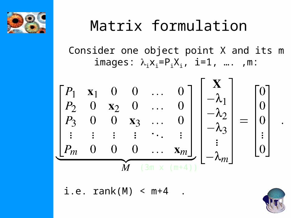
Matrix formulation

Consider one object point X and its m images: ixi=PiXi, i=1, …. ,m:

i.e. rank(M) < m+4 .

(3m x (m+4))

Laplace expansions

• The rank condition on M implies that all (m+4)x(m+4) minors of M are equal to 0.

• These can be written as sums of products of camera matrix parameters and image coordinates.

det

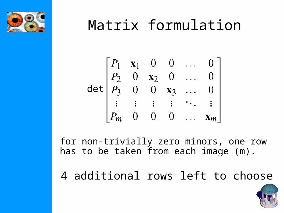
Matrix formulation

for non-trivially zero minors, one row has to be taken from each image (m).

4 additional rows left to choose

det

0

000000000000000

lk

jihgfedcba

0

ihgfedcba

jkl

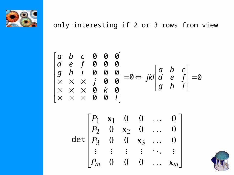
only interesting if 2 or 3 rows from view

det

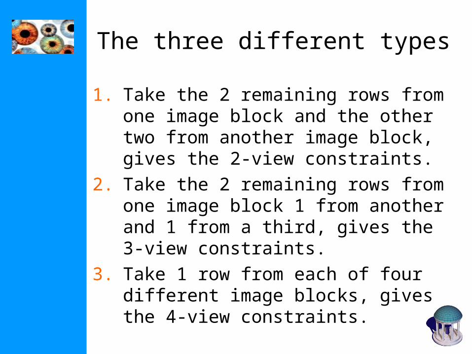
The three different types

1. Take the 2 remaining rows from one image block and the other two from another image block, gives the 2-view constraints.

2. Take the 2 remaining rows from one image block 1 from another and 1 from a third, gives the 3-view constraints.

3. Take 1 row from each of four different image blocks, gives the 4-view constraints.

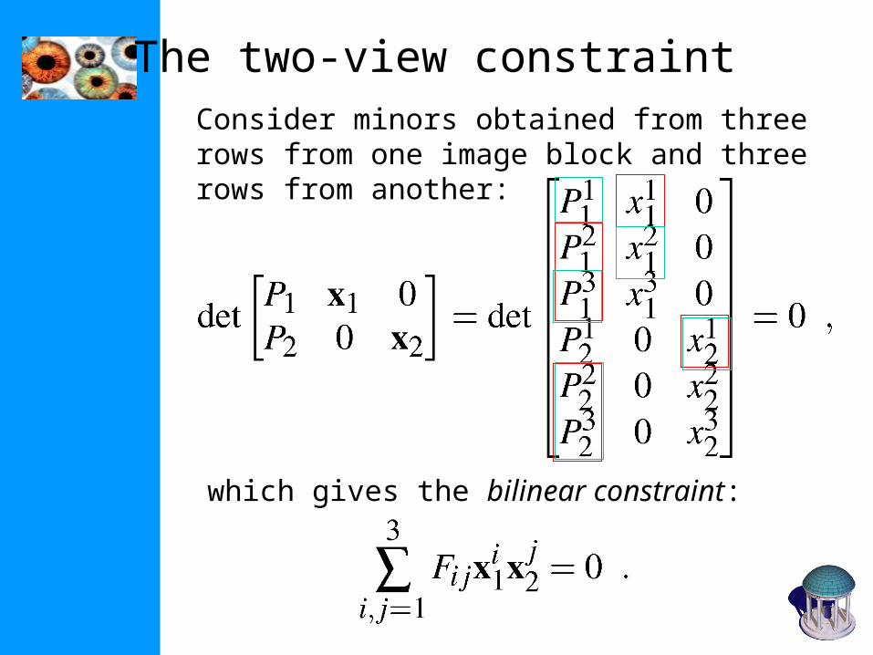
The two-view constraintConsider minors obtained from three rows from one image block and three rows from another:

which gives the bilinear constraint:

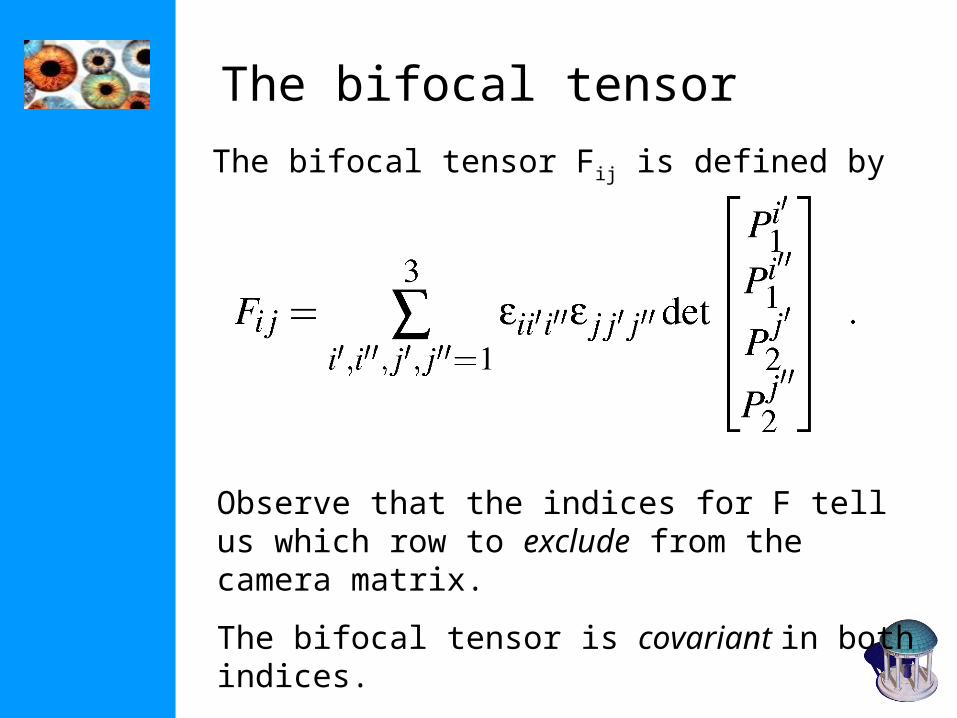
The bifocal tensor

The bifocal tensor Fij is defined by

Observe that the indices for F tell us which row to exclude from the camera matrix.

The bifocal tensor is covariant in both indices.

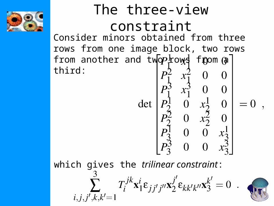
The three-view constraintConsider minors obtained from three rows from one image block, two rows from another and two rows from a third:

which gives the trilinear constraint:

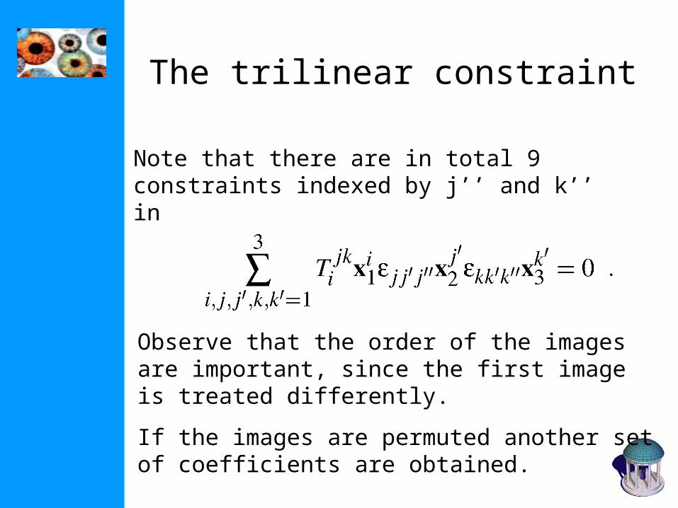
The trilinear constraint

Note that there are in total 9 constraints indexed by j’’ and k’’ in

Observe that the order of the images are important, since the first image is treated differently.

If the images are permuted another set of coefficients are obtained.

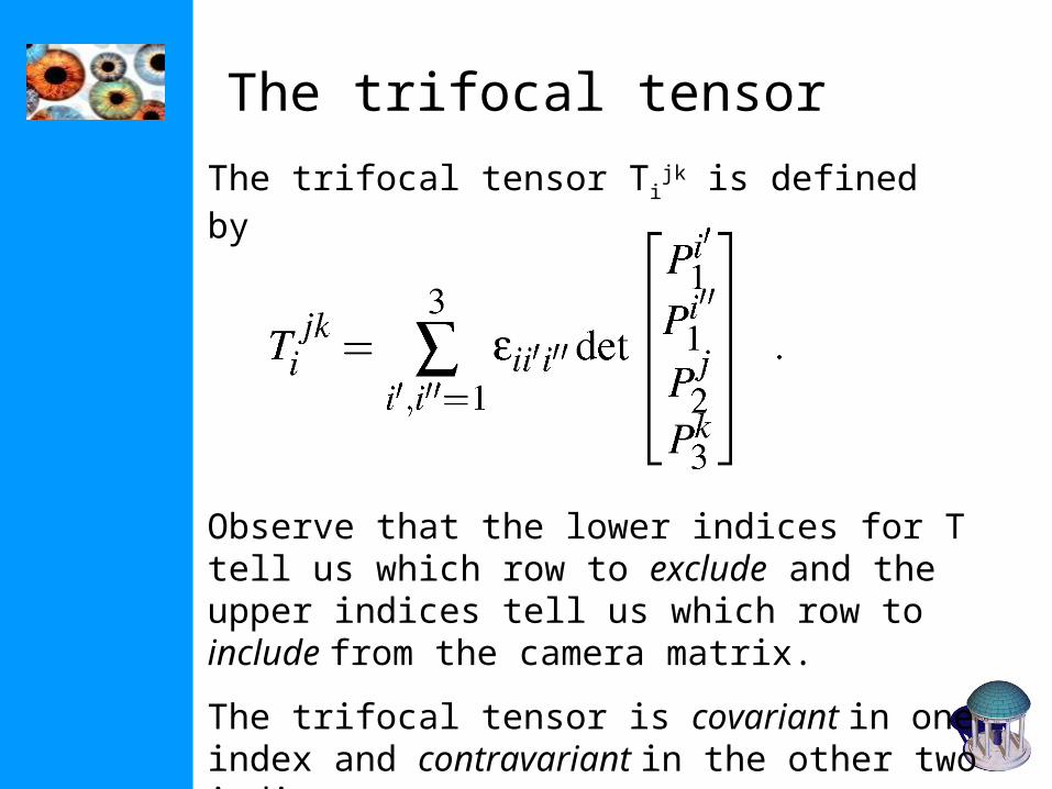
The trifocal tensor

The trifocal tensor Tijk is defined by

Observe that the lower indices for T tell us which row to exclude and the upper indices tell us which row to include from the camera matrix.

The trifocal tensor is covariant in one index and contravariant in the other two indices.

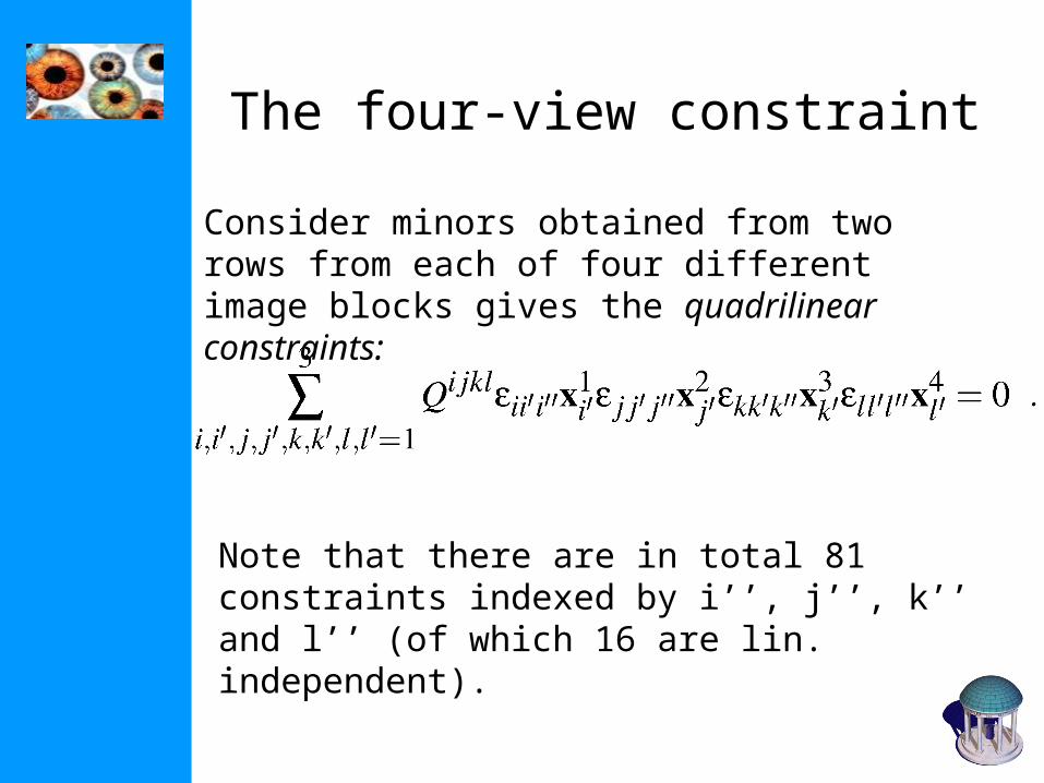
The four-view constraint

Consider minors obtained from two rows from each of four different image blocks gives the quadrilinear constraints:

Note that there are in total 81 constraints indexed by i’’, j’’, k’’ and l’’ (of which 16 are lin. independent).

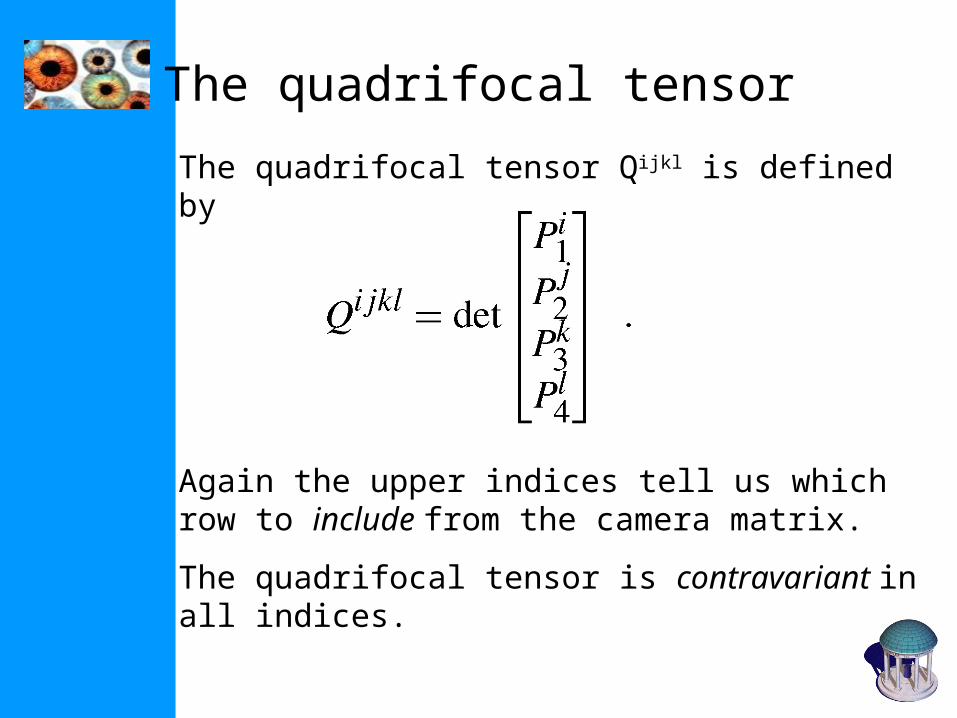
The quadrifocal tensor

The quadrifocal tensor Qijkl is defined by

Again the upper indices tell us which row to include from the camera matrix.

The quadrifocal tensor is contravariant in all indices.

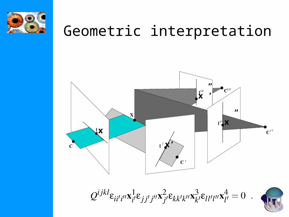
Geometric interpretation

x

x’

x”

x”’

The quadrifocal tensor and lines

0 pqrssrqp Qllll

Lines do not have to come from same 3D line, but only have to pass through same point

Self-calibration

Outline

• Introduction• Self-calibration• Dual Absolute Quadric• Critical Motion Sequences

Motivation

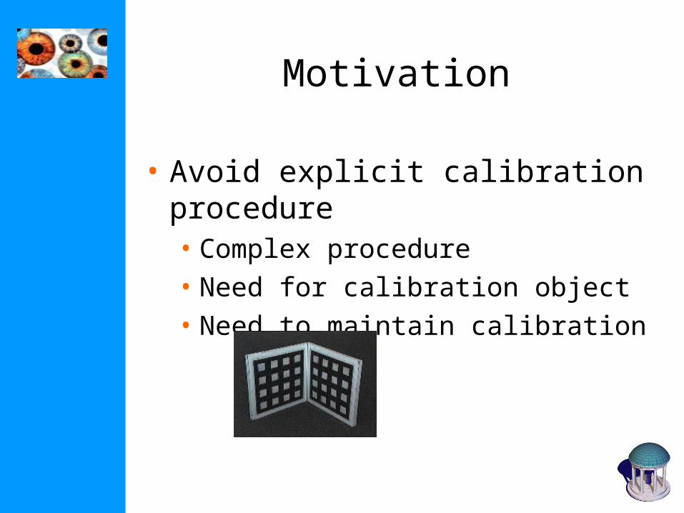
• Avoid explicit calibration procedure• Complex procedure• Need for calibration object • Need to maintain calibration

Motivation

• Allow flexible acquisition• No prior calibration necessary• Possibility to vary intrinsics• Use archive footage

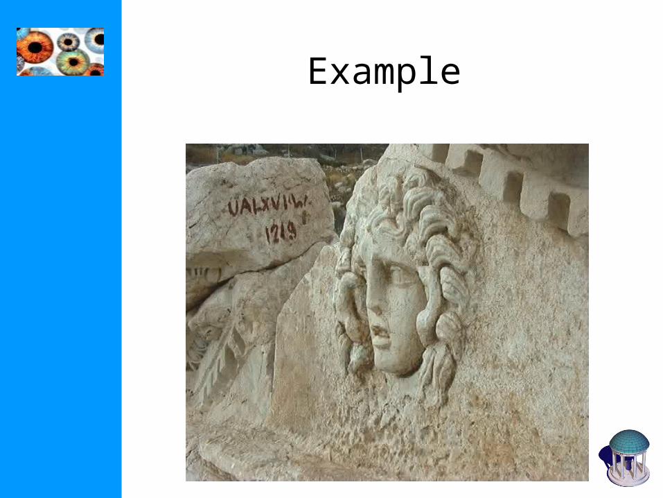
Example

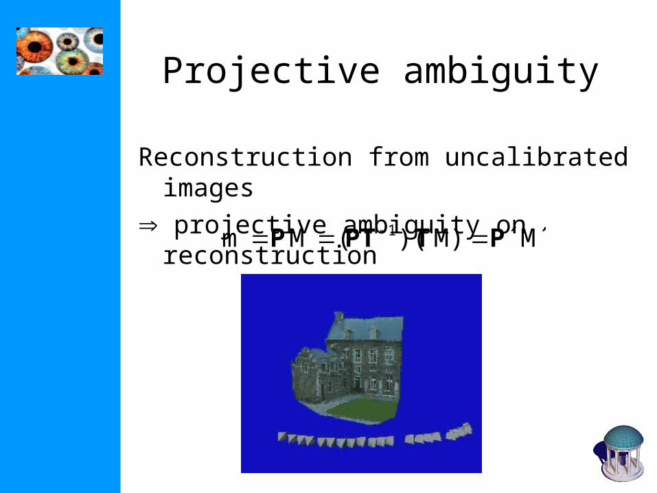
Projective ambiguity

Reconstruction from uncalibrated images

projective ambiguity on reconstruction

´M´M))((Mm 1 PTPTP

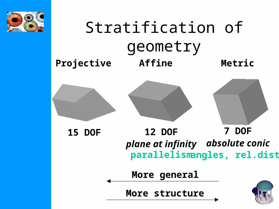
Stratification of geometry

15 DOF 12 DOFplane at infinity

parallelism

More general

More structure

Projective Affine Metric

7 DOFabsolute conicangles, rel.dist.

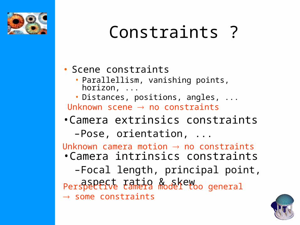
Constraints ?

• Scene constraints• Parallellism, vanishing points, horizon, ...• Distances, positions, angles, ...Unknown scene no constraints

• Camera extrinsics constraints–Pose, orientation, ...

Unknown camera motion no constraints • Camera intrinsics constraints

–Focal length, principal point, aspect ratio & skew

Perspective camera model too general some constraints

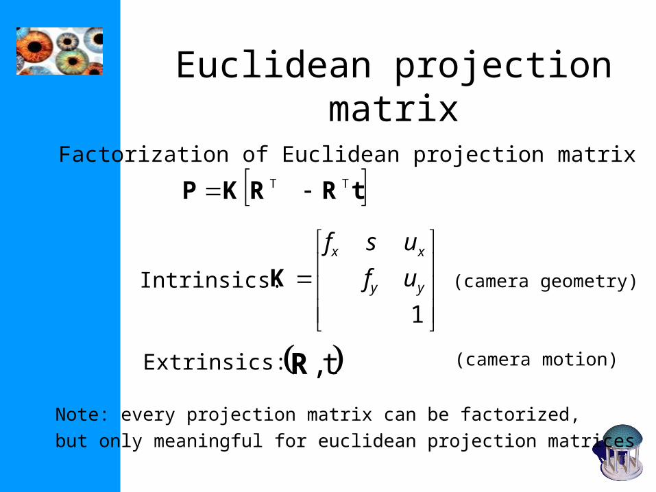
Euclidean projection matrix

tRRKP TT

1yy

xx

uf

usf

K

Factorization of Euclidean projection matrix

Intrinsics:

Extrinsics: t,R

Note: every projection matrix can be factorized,

but only meaningful for euclidean projection matrices

(camera geometry)

(camera motion)

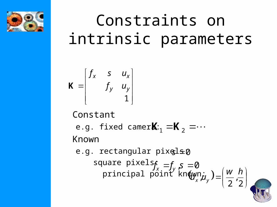
Constraints on intrinsic parameters

Constant e.g. fixed camera:

Knowne.g. rectangular pixels:

square pixels: principal point known:

21 KK

0s

1yy

xx

uf

usf

K

0, sff yx

2,

2,

hwuu yx

Self-calibration

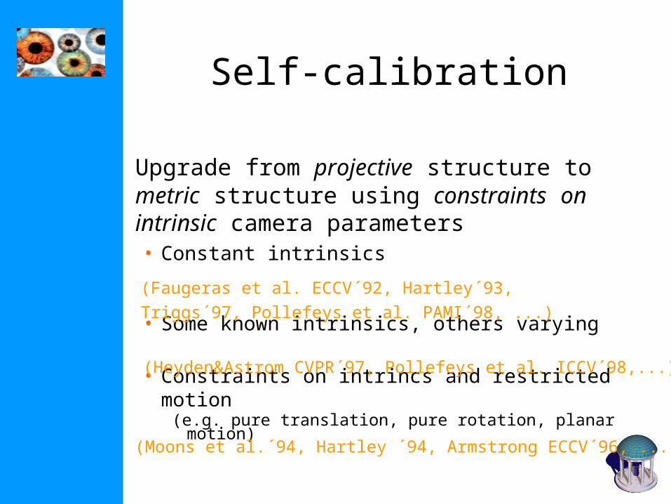
Upgrade from projective structure to metric structure using constraints on intrinsic camera parameters• Constant intrinsics

• Some known intrinsics, others varying

• Constraints on intrincs and restricted motion(e.g. pure translation, pure rotation, planar motion)

(Faugeras et al. ECCV´92, Hartley´93,

Triggs´97, Pollefeys et al. PAMI´98, ...)

(Heyden&Astrom CVPR´97, Pollefeys et al. ICCV´98,...)

(Moons et al.´94, Hartley ´94, Armstrong ECCV´96, ...)

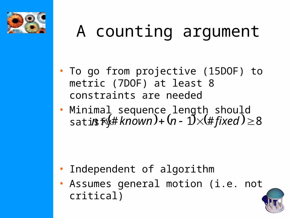
A counting argument

• To go from projective (15DOF) to metric (7DOF) at least 8 constraints are needed

• Minimal sequence length should satisfy

• Independent of algorithm• Assumes general motion (i.e. not critical)

8#1# fixednknownn

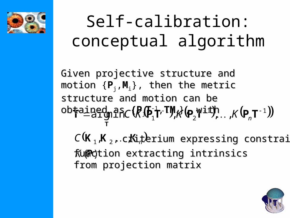
Self-calibration:conceptual algorithm

112

11 ,,,minarg TPTPTPT

TnKKKC

)(

,,, 21

P

KKK

K

C n criterium expressing constraints criterium expressing constraints

function extracting intrinsics function extracting intrinsics from projection matrixfrom projection matrix

Given projective structure and motion Given projective structure and motion {Pj,Mi},

then the metric structure and motion can be then the metric structure and motion can be obtained as obtained as {PjT-1,TMi}, with with

Outline

• Introduction• Self-calibration• Dual Absolute Quadric• Critical Motion Sequences

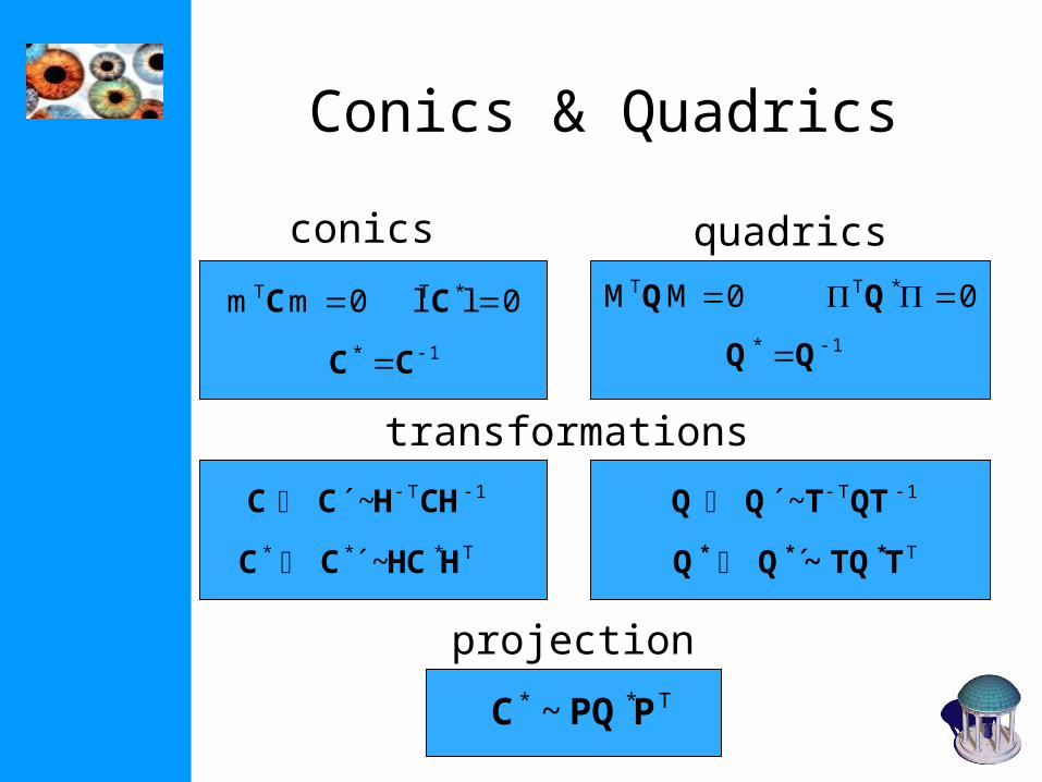
Conics & Quadrics

0mmT C 0ll *T C

1* CC

conics

0MMT Q 0*T Q

1* QQ

quadrics

1T´~ CHHCC

T*** ´~ HHCCC T´ TTQ~QQ ***

1T´~ QTTQQ

transformations

T** ~ PPQC

projection

The Absolute Dual Quadric

Degenerate dual quadric *

Encodes both absolute conic and

*

0π0

π

T

T

0

0Ifor metric frame:

(Triggs CVPR´97)

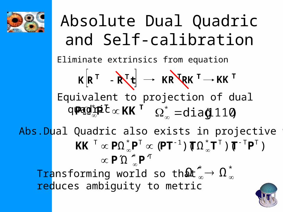
Absolute Dual Quadric and Self-calibration

Eliminate extrinsics from equation

Equivalent to projection of dual quadric

))(Ω)((Ω *1* TTTTT PTTTPTPPKK

Abs.Dual Quadric also exists in projective world

T´Ω´´ * PP Transforming world so thatreduces ambiguity to metric

** ΩΩ´

*

*

projection

constraints

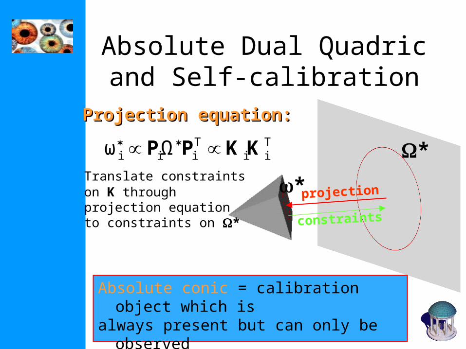
Absolute conic = calibration object which is always present but can only be observed through constraints on the intrinsics

Tii

Tiii Ωω KKPP

Absolute Dual Quadric and Self-calibration

Projection equation:Projection equation:

Translate constraints on K through projection equation to constraints on *

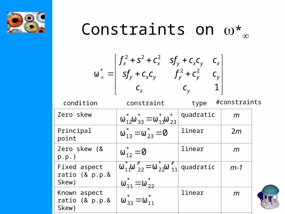
Constraints on *

1

ω 22

222

*

yx

yyyyxy

xyxyxx

cc

ccfccsf

cccsfcsf

Zero skew quadratic m

Principal point linear 2m

Zero skew (& p.p.)

linear m

Fixed aspect ratio (& p.p.& Skew)

quadratic m-1

Known aspect ratio (& p.p.& Skew)

linear m

Focal length (& p.p. & Skew)

linear m

*23

*13

*33

*12 ωωωω

0ωω *23

*13

0ω*12

*11

*22

*22

*11 ω'ωω'ω

*22

*11 ωω

*11

*33 ωω

condition constraint type #constraints

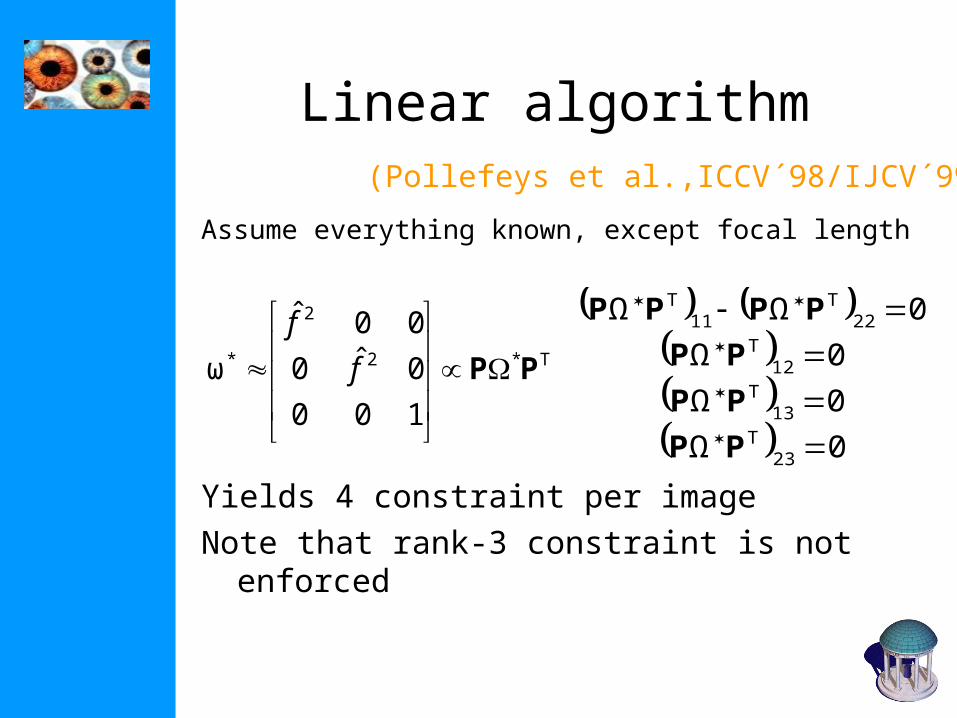
Linear algorithm

Assume everything known, except focal length

0Ω

0Ω

0Ω

0ΩΩ

23T

13T

12T

22T

11T

PP

PP

PP

PPPP

(Pollefeys et al.,ICCV´98/IJCV´99)

TPP *2

2

*

100

0ˆ0

00ˆ

ω

f

f

Yields 4 constraint per imageNote that rank-3 constraint is not enforced

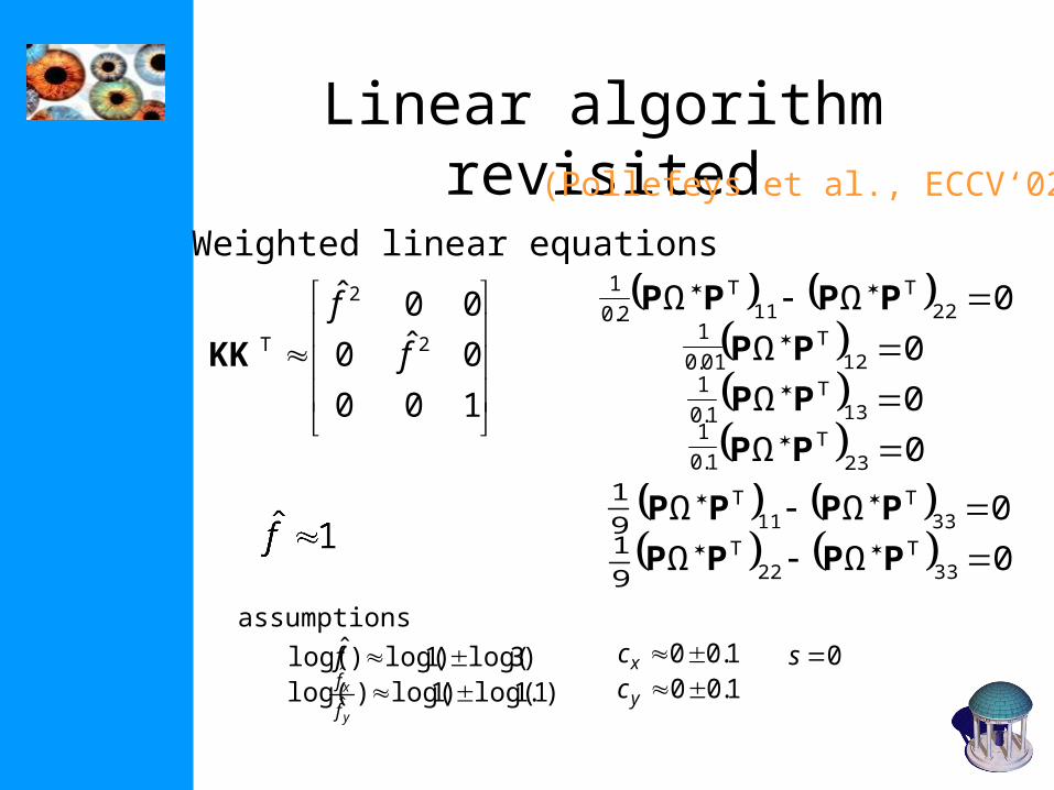
Linear algorithm revisited

0Ω

0Ω

0Ω

0ΩΩ

23T

13T

12T

22T

11T

PP

PP

PP

PPPP

100

0ˆ0

00ˆ2

2

f

fTKK

9

1

9

1

)3log()1log()ˆlog( f)1.1log()1log()log( ˆ

ˆ

y

x

f

f1.00xc1.00yc

0s

0ΩΩ

0ΩΩ

33T

22T

33T

11T

PPPP

PPPP

(Pollefeys et al., ECCV‘02)

1.0

11.0

101.0

12.0

1

assumptions

Weighted linear equations

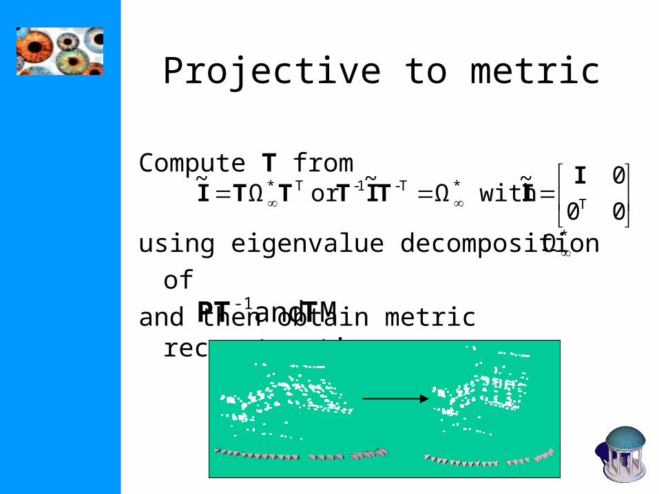
Projective to metric

Compute T from

using eigenvalue decomposition of and then obtain metric

reconstruction as

00

0

~ withΩ

~or Ω

~ **T

T-1-T IITITTTI

M and TPT-1

Ω*

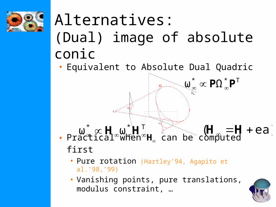
Alternatives: (Dual) image of absolute conic

• Equivalent to Absolute Dual Quadric

• Practical when H can be computed first• Pure rotation (Hartley’94, Agapito et al.’98,’99)

• Vanishing points, pure translations, modulus constraint, …

T** ωω HH ea)( HH

TPP ** Ωω

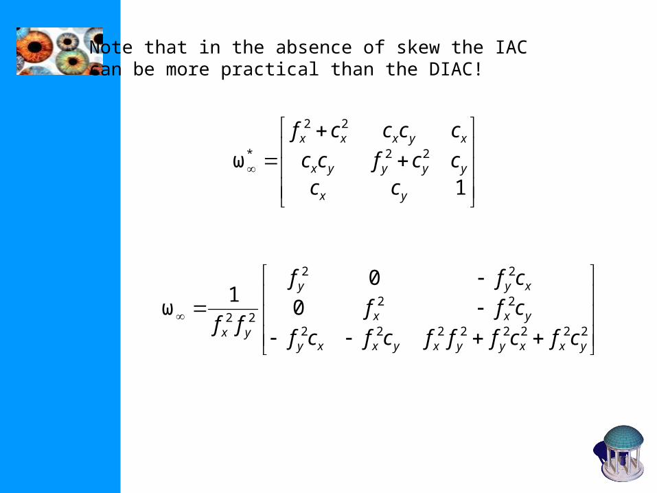
1ω 22

22

*

yx

yyyyx

xyxxx

ccccfcc

ccccf

22222222

22

22

220

01

ω

yxxyyxyxxy

yxx

xyy

yx cfcfffcfcf

cff

cff

ff

Note that in the absence of skew the IAC can be more practical than the DIAC!

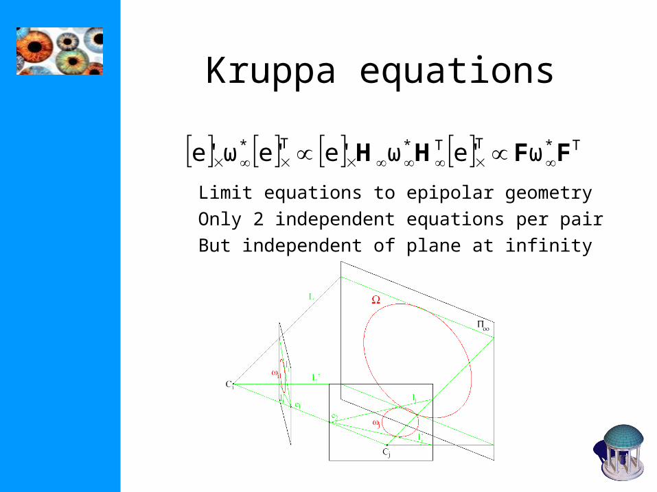
Kruppa equations

Limit equations to epipolar geometryOnly 2 independent equations per pairBut independent of plane at infinity

T*TT*T* ωe'ωe'e'ωe' FFHH

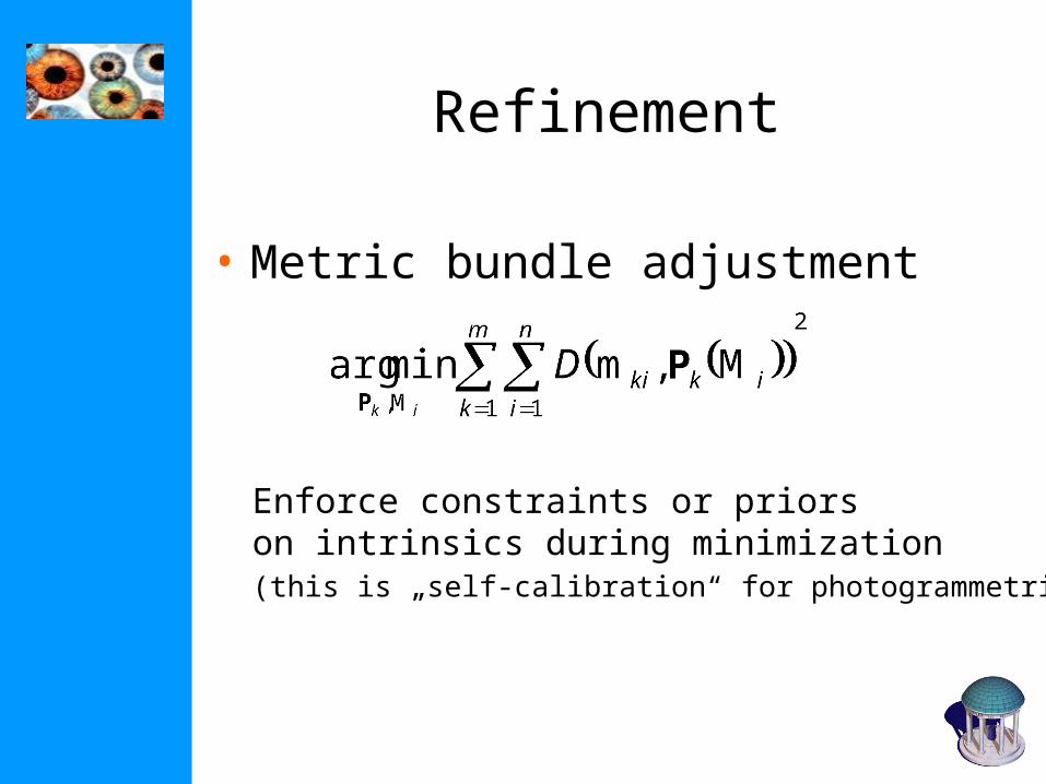
Refinement

• Metric bundle adjustment

Enforce constraints or priors on intrinsics during minimization(this is „self-calibration“ for photogrammetrist)

Outline

• Introduction• Self-calibration• Dual Absolute Quadric• Critical Motion Sequences

Critical motion sequences

• Self-calibration depends on camera motion• Motion sequence is not always general

enough

• Critical Motion Sequences have more than one potential absolute conic satisfying all constraints

• Possible to derive classification of CMS

(Sturm, CVPR´97, Kahl, ICCV´99, Pollefeys,PhD´99)

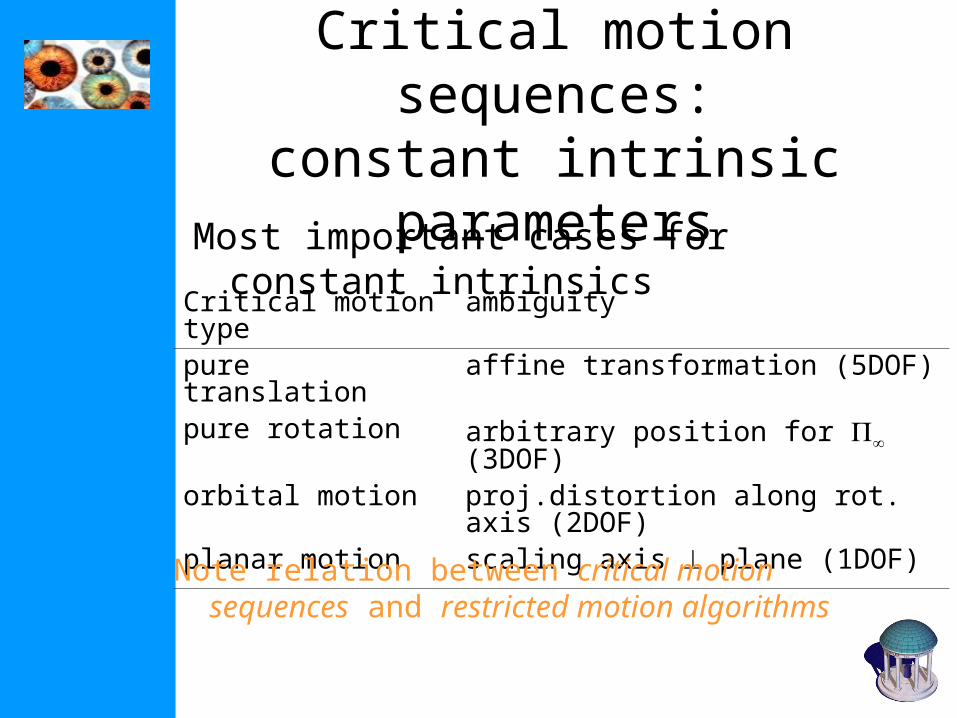
Critical motion sequences:constant intrinsic parameters

Most important cases for constant intrinsics

Critical motion type

ambiguity

pure translation affine transformation (5DOF)pure rotation arbitrary position for (3DOF)orbital motion proj.distortion along rot. axis

(2DOF)planar motion scaling axis plane (1DOF)

Note relation between critical motion sequences and restricted motion algorithms

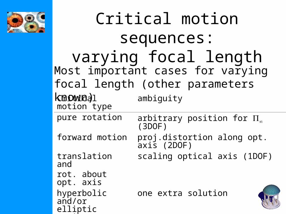
Critical motion sequences:varying focal length

Most important cases for varying focal length (other parameters known)Critical motion type

ambiguity

pure rotation arbitrary position for (3DOF)forward motion proj.distortion along opt. axis

(2DOF)translation and rot. about opt. axis

scaling optical axis (1DOF)

hyperbolic and/or elliptic motion

one extra solution

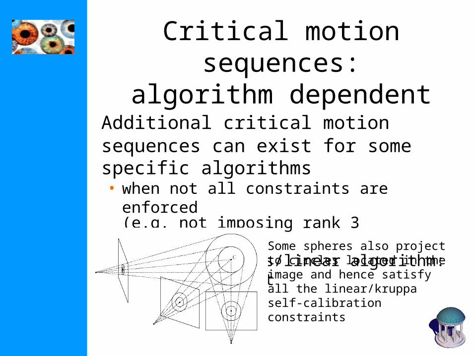
Critical motion sequences:algorithm dependent

Additional critical motion sequences can exist for some specific algorithms• when not all constraints are enforced

(e.g. not imposing rank 3 constraint)• Kruppa equations/linear algorithm: fixating

a pointSome spheres also project to circles located in the image and hence satisfy all the linear/kruppa self-calibration constraints

Non-ambiguous new views for CMS

• restrict motion of virtual camera to CMS• use (wrong) computed camera parameters

(Pollefeys,ICCV´01)

Next class: Multiple View Reconstruction