self-organized criticality in developing neuronal networks

Self-Organized Criticality in Developing NeuronalNetworksChristian Tetzlaff1*, Samora Okujeni2, Ulrich Egert2, Florentin Worgotter1, Markus Butz3

1 Bernstein Center for Computational Neuroscience, Institute of Physics III - Biophysics, Georg-August Universitat, Gottingen, Germany, 2 Bernstein Center for

Computational Neuroscience, Albert-Ludwigs Universitat, Freiburg, Germany, 3 Neuroinformatics Group, Neuroscience Campus, VU Universiteit, Amsterdam, The

Netherlands

Abstract

Recently evidence has accumulated that many neural networks exhibit self-organized criticality. In this state, activity issimilar across temporal scales and this is beneficial with respect to information flow. If subcritical, activity can die out, ifsupercritical epileptiform patterns may occur. Little is known about how developing networks will reach and stabilizecriticality. Here we monitor the development between 13 and 95 days in vitro (DIV) of cortical cell cultures (n = 20) and findfour different phases, related to their morphological maturation: An initial low-activity state (<19 DIV) is followed by asupercritical (<20 DIV) and then a subcritical one (<36 DIV) until the network finally reaches stable criticality (<58 DIV).Using network modeling and mathematical analysis we describe the dynamics of the emergent connectivity in suchdeveloping systems. Based on physiological observations, the synaptic development in the model is determined by thedrive of the neurons to adjust their connectivity for reaching on average firing rate homeostasis. We predict a specific timecourse for the maturation of inhibition, with strong onset and delayed pruning, and that total synaptic connectivity shouldbe strongly linked to the relative levels of excitation and inhibition. These results demonstrate that the interplay betweenactivity and connectivity guides developing networks into criticality suggesting that this may be a generic and stable stateof many networks in vivo and in vitro.

Citation: Tetzlaff C, Okujeni S, Egert U, Worgotter F, Butz M (2010) Self-Organized Criticality in Developing Neuronal Networks. PLoS Comput Biol 6(12):e1001013. doi:10.1371/journal.pcbi.1001013

Editor: Karl J. Friston, University College London, United Kingdom

Received April 11, 2010; Accepted October 27, 2010; Published December 2, 2010

Copyright: � 2010 Tetzlaff et al. This is an open-access article distributed under the terms of the Creative Commons Attribution License, which permitsunrestricted use, distribution, and reproduction in any medium, provided the original author and source are credited.

Funding: The project was supported by BCCN grants from the German ministry for research and education (BMBF) via the Bernstein Center for ComputationalNeuroscience (BCCN) Gottingen as well as Freiburg. F.W. acknowledges BMBF BFNT funding (Project 3a), and M.B. from the Computational Life Sciencesprogramme grant (635.100.017) of the Netherlands Organization for Research (NWO). The funders had no role in study design, data collection and analysis,decision to publish, or preparation of the manuscript.

Competing Interests: The authors have declared that no competing interests exist.

* E-mail: [email protected]

Introduction

During the last years increasing evidence has accumulated that

networks in the brain can exhibit ‘‘self-organized criticality’’ [1–3].

Self-organized criticality is one of the key concepts to describe the

emergence of complexity in nature and has been found in many

systems – ranging from the development of earthquakes [4] to

nuclear chain reactions [5]. All these systems exhibit spatial and

temporal distributions of cascades of events called avalanches

which can be well described by power laws [6–8]. This indicates

that the system is in a critical state [6,9] and that similar dynamic

behavior exists across many different scales. Several neural

network models have predicted that neural activity might also

been organized this way [10–14] and recently this had been

confirmed experimentally [1,15–17]. A recent study by Levina and

colleagues [18] addresses the question how self-organized

criticality can emerge in such networks in a robust way by using

dynamical synapses, which alter their synaptic connection strength

on a fast time scale. This contribution, which is able to analytically

predict the network behavior, is a theoretical milestone in our

understanding of criticality in neural systems. In general, however,

theoretical and experimental investigations have so far usually

focused on mature networks [1,16] sometimes including adaptive

processes [18–20]. Little is known how developing networks can

reach a final state of self-organized criticality [10,17,21]. In the

current paper, we are therefore experimentally investigating the

different stages of developing cortical cell cultures [22] to assess

under which conditions these networks develop into a critical state.

Specifically we are asking the following questions: 1) do the

investigated cell cultures undergo a significant transition in their

activity states and how is this related to self-organized criticality

and 2) can specific predictions be made with respect to network

activity and connectivity which would explain the observed

behavior. To address the second aspect we are designing a model

to simulate network development, which is based on activity-

dependent axonal and dendritic growth leading to homeostasis in

neuronal activity [23–28].

Results

Experimental approachIn order to assess how self-organized criticality develops in cell

cultures, we have monitored a total of 20 cultures and recorded

their activity patterns between 13 and 95 days in vitro (DIV). In

general, cultures start with about 500,000 dissociated cortical

neurons, which develop over time into an interconnected network.

To assess the different network states the activity at 59 electrodes

was measured and analyzed at different DIV (see Methods).

PLoS Computational Biology | www.ploscompbiol.org 1 December 2010 | Volume 6 | Issue 12 | e1001013

Figure 1 A shows 15 minutes of recorded activity for one typical

culture at 42 DIV. At this temporal resolution individual bursts are

visible as vertical dot-lines indicating activity at almost all

electrodes, separated by rather long pauses which allow for robust

separation of these bursts required for avalanche analysis. At a fine

temporal resolution (Figure 1 B) one sees that the burst activity

expresses certain patterns. Note, pauses have been graphically

shortened in panels (B) and (C). Panel (C) shows the activity

pattern that arises in our model, which at a first glance looks

similar to that in the culture. Details about the model and an

analysis which support similarity of model and real data, will be

provided later. First we would like to describe the developmental

stages in the cultures with respect to their avalanche distributions.

In this work, avalanches are defined by the number of spikes

between two windows without activity (see Methods).

At early stages during development, usually before 13 DIV,

connectivity is small and activity in the network very low. So, it is

very difficult to obtain long enough recordings for plotting

avalanche distributions. However, known from the literature

[29], in this stage activity is best described by a Poisson like

behavior. At about 13 DIV (see Figure 2), we receive the first

distributions which develop towards criticality (Figure 3 A).

Therefore, we call this state the initial state. The ideal power-law

fit for each curve is shown by the dashed lines. If a distribution

matches the power law line it can be called ‘‘critical’’ [6,7]. A

dominance of long avalanches is indicative of a supercritical state

whereas a lack thereof is referred to as subcritical. This is

measured by Dp, which gives the quality of fit between ideal power

law and actual distribution. For a system in a supercritical state Dpis larger and for a subcritical state smaller than zero (see

Methods). Values of Dp are also shown in the different panels

of Figure 3. For the cultures, we receive at (on average) 19 DIV

values of Dp in the interval from {0:19 to {0:38. While this

shows that the system develops towards criticality, we also

observed that this behavior is very unstable. Quickly, within just

(on average) one/two days, the distributions change shape and

develop a substantial ‘‘bump’’ for larger avalanches. This indicates

that at (on average) 22 DIV the network enters a supercritical

regime (Figure 3 B). After (on average) 36 DIV network activity is

curbed and it reaches a subcritical regime (Figure 3 C). This can

be seen by the decrease of the distribution at larger avalanches. At

(on average) 58 DIV the system becomes finally critical (Figure 3

d). Here we find that the deviation from a power law is nearly zero

(for these examples Dp~{0:06+0:17). In general we find that

the differences between all states are significant for the measured

values of Dp (ANOVA test). Figure 2 provides the data of all 20

cultures (see Methods) divided into the different states. All

completely measured cultures undergo the same transitions from

initial (black) to supercritical (red) to subcritical (green) and finally

to a critical state (blue). The overlap between the first two states

results from the very quick transition between them together with

small differences in the speed of development of the different

cultures. Average values of Dp for these four states are {0:28,

1:42, {0:91, and {0:06 (see Table in Figure 2). Differences are

significant using the multiple comparison procedure with Bonfer-

roni correction based on the one-way ANOVA test. Only the

difference between the initial and critical state is not significant as

in the initial state the network develops towards criticality until

strong morphological changes set in (see Phase I). However, the

activity given by the number of action potentials per minute is for

the supercritical state significantly higher than for the initial,

subcritical and critical state, which has the lowest mean activity.

These were the only differences that were observed.

In summary, these results show that there is a characteristic time

course in the development of the avalanche distributions. The

Figure 1. Raster plots at different temporal resolutions forexperimental and model data. They are showing (A) the patterns ofhigh burst-like activity and following pauses and (B,C) the activitypatterns during some bursts. For graphical reasons, in panels (B,C)intervals between bursts have been shortened and do not correspondto the true intervals visible in panel (A). Thus scale bars refer only to thebursts.doi:10.1371/journal.pcbi.1001013.g001

Author Summary

Learning depends crucially on the synaptic distribution ina neural network. Therefore, investigating the develop-ment from which a certain distribution emerges is crucialfor our understanding of network function. Morphologicaldevelopment is controlled by many different parameters,most importantly: neuronal activity, synapse formation, andthe balance between excitation and inhibition, but it islargely unknown how these parameters interact ondifferent time scales and how they influence the develop-ing network structure. In our work, we consider the well-known concept of self-organized criticality. We havemeasured how real cell cultures change their activitypatterns during the first 60 days of development traversingthrough different stages of criticality. With a dynamicmodel we can reproduce the observed developmentalstates and predict specific time-courses for the networkparameters. For example, the model predicts a delayed,overshooting onset of inhibition with a longer time toreach maturation as compared to excitation. Furthermore,we suggest that the balance of dendrites and axons in themature state is quite sensitive to the initial conditions ofdevelopment. These and several more predictions areaccessible by future experimental work and can help us tobetter understand neuronal networks and their parametersduring development and also in the mature state.

Criticality in Developing Networks


system starts with low activity and then enters a transitory initial

state. Quickly it leaves this state and, passing supercritical and

subcritical regimes, reaches the critical state.

Modelling approachNeurite growth and retraction towards firing rate

homeostasis. The model uses two opposing mechanisms of

axonal and dendritic growth and is driven by the goal to reach

homeostasis of the mean firing rate. The first mechanism regulates

dendritic growth probabilities inversely to neuronal activity and

the second is the axonal outgrowth promoted by activity. Specific

choices for the model are being discussed in the Discussion section,

where we also summarize the different specific predictions made

by the model and described in detail in the next sections.

As will be shown below, the model is capable of reproducing all

different patterns of neuronal activity (Figure 3) based on the

implemented rules for activity-dependent structural network

formation. A neuron is represented by its membrane potential jti

and its inner calcium concentration cti (see Methods) at the time

point t. After a disturbance, these variables will decay in time to

the resting values j0 and 0 for the membrane potential and the

calcium concentration, respectively. Every time a neuron gener-

ates an action potential (see Equation 15 in Methods), its calcium

concentration increases by a constant b.

Dependent on the difference between the current calcium

concentration and a desired homeostatic value ctarget, the neuron

changes its input (dendritic acceptance dti ) and output (axonal

supplies ati ) by ways of a simulated growth or withdrawal process

(see Methods). The intersection between input and output of two

neurons i and j determines the synaptic density stij , and hence the

connectivity, between them.

The difference between an inhibitory and excitatory neuron is

defined by constants kinhv0 and kexc

w0, which are prefactors

of stij .

In summary, the model comprises a negative feedback loop of

the following kind (Figure 4 A): Neuronal activity (1) determines

the calcium level (2) in the cell. This level leads to the simulated

growth pattern of the neuron(s). The growth pattern determines

the effective amount of axonal supplies and dendritic acceptances

(3). Thus, growth of many neurons, influencing their respective

neuritic offers, will lead to different synaptic densities (4) between

neurons. We use this synaptic density as the simplest way to

estimate the inputs (5) to any given cell. This input will then

determine the cell’s activity closing the loop at (1).

These interactions lead to the effect that the model development

passes through three different morphological phases (Figure 4 B–

D), which we will first describe qualitatively and in the following

subsections also analyze mathematically as far as possible.

The initial supplies of the axons and acceptances of the

dendrites are chosen such that no connections exist. As a

consequence of the resulting too low activity the dendritic

acceptance increases to build synapses and to enhance the activity

in the first developmental phase I. It rises slowly and, at a certain

point in time, increases explosively towards a maximum. Parallel

to this increase in activity, the system undergoes a morphological

transition (Phase II) until it reaches homeostasis (Phase III). As

discussed later (see Discussion), this is similar to the morpho-

logical development in such cultures (see inset in Figure 4 B). At

the final stage the mean activity is equal to the homeostatic value

(see Methods) and changes of the axonal supplies and dendritic

acceptances are negligible.

The three different phases in the above described development

can be largely understood in an analytical way and we can also

describe to what degree the system approaches criticality. The

difficult recurrent processes, which drive the interactions within a

network and lead to a specific avalanche distribution, however,

defy analytical analysis and can only be obtained from simulations.

Additionally, the effects of inhibition on the network dynamic in

the different developmental phases are tested by simulations.

Phase I: First developmental phase F(St)v1

tj

� �The first phase (Phase I) of the network development is

characterized by dendritic growth to establish first synaptic

contacts and to rise neuronal activities. At the beginning of the

model development the dendritic acceptance increases (Figure 4

C). By this outgrowth the system creates synapses and forms a

network. The distribution of the avalanches, the mean membrane

potential Jt, and the mean calcium concentration Ct also changes

(mean values over all neurons are given as upper case letters, while

lower case letters indicate individual values). Similar to real cell

Figure 2. Development of the deviation from a power law Dp of cell cultures. The transitions from initial (black) to supercritical (red) tosubcritical (green) and critical state (blue) can be clearly seen. Data from the same cell culture at different time points are connected. 14% of the totalnumber of cultures has been tracked at 5 different time points, 7% at 4 time points, 29% at 3, 14% at 2, and 36% once. Squares indicate the mean

values of DIV and Dp (+ indicates the standard deviation), which are given in the inset Table, of the associated state.AP

minamount of action potentials

per minute, therefore, mean activity.doi:10.1371/journal.pcbi.1001013.g002



cultures, all neurons at this phase are excitatory. With the help of a

mean field approach it is possible to calculate average membrane

potential Jt and average calcium concentration Ct during this

phase. Different from real networks, where the activity is too small

to render reliable measurements for very early developmental

stages, in the model we can also analyze these. For this, the term

PNj~1kc st

ij H jtj{%t

j

� �, which determines the increase of the

membrane potential jti according to the activity of the connected

neurons j in Equation 14 (see Methods), is simplified to a product

of the mean membrane potential Jt and an monotonous function

dependent on the mean synaptic density F (St) (see below) and we

get for the activity change:

Figure 3. Avalanche distribution changes during morphological development of dissociated cell cultures. The dashed line indicates aperfect power law distribution. The deviation of the cell culture data from this line measures the criticality of these systems. For each state threedifferent examples are shown. The age of each state of the cell cultures is given in the bottom right corner of the panels. (A) Initial state (on average19 DIV); (B) supercritical state showing a ‘‘bump’’ of many long avalanches (on average 22 DIV); (C) subcritical state (on average 36 DIV) showing adepression and hence a lack of long avalanches; and (D) critical state (on average 58 DIV) with a good match to the power law line.doi:10.1371/journal.pcbi.1001013.g003



dJt

dt~

j0

tjzJt: F (St){

1

tj

� �: ð1Þ

The differential equation of the calcium concentration (Equation

15 in Methods) can be written as:

dCt

dt~{

Ct

tC

zbJt: ð2Þ

With these equations, we can now consider three different degrees

of synaptic densities in the first phase F (St)v1

tj

� �; namely zero,

small, and medium densities and for Phase II F (St)§1

tj

� �with a

large density.

Network development before synapse formation

F(St)~0� �

. For the initial conditions of the model without

connectivity, F (St) is set to zero. Therefore, from Equation 1 one

can obtain that the mean activity Jt reaches the resting potential:

limt??

Jt~j0: ð3Þ

If this solution is entered in Equation 2, we get:

limt??

Ct~bj0tC : ð4Þ

Thus, also the mean calcium concentration reaches a constant

value dependent on j0.

Taking the limit t?? corresponds to letting the system under

the given condition F (St)~0 relax into its end state. Note

however, that the actually ongoing development (Figure 4 A) will

curtail this condition as eventually 0vF (St)v1=tj.

From Figure 5 A we can see that the avalanche distribution

shows a poissonian form. This is also reflected by a large negative

value for Dp (Table 1, first row). This changes as soon as the model

begins to make the first connections between neurons as shown in

the following.

Network development with small and medium

connectivity F(St)vv1

tj

� �. As soon as the system has reached

small connectivity, the behavior of the membrane potential, calcium

concentration, and avalanche distribution changes. This

corresponds to a situation where we have F (St) larger than zero

but smaller than1

tj. So, the system is still in Phase I. It is easy to see

that the dynamics change again if the density function becomes

larger than1

tjand this is later discussed in Phase II.

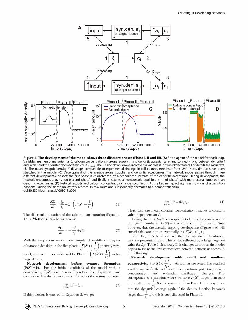
Figure 4. The development of the model shows three different phases (Phase I, II and III). (A) Box diagram of the model feedback loop.Variables are membrane potential ji , calcium concentration ci , axonal supply ai and dendritic acceptance di , and connectivity sij between dendrite iand axon j and the constant homeostatic value ctarget. The up and down arrows indicate if a variable is increased/decreased. For details see main text.(B) The mean synaptic density S develops comparable to experimental findings in cell cultures (see inset from [24]). Note, time axis has beenstretched in the middle. (C) Development of the average axonal supplies and dendritic acceptances. The network model passes through threedifferent developmental phases: the first phase is characterized by a pronounced increase of the dendritic acceptance. During development, thenetwork undergoes a transition (second phase) and finally it reaches a homeostatic equilibrium (third phase) with more axonal supplies thandendritic acceptances. (D) Network activity and calcium concentration change accordingly. At the beginning, activity rises slowly until a transitionhappens. During the transition, activity reaches its maximum and subsequently decreases to a homeostatic value.doi:10.1371/journal.pcbi.1001013.g004



We can solve the differential equations (Equation 14 and 15) for

the mean variables with standard methods and get:

limt??

Jt~j0

1{tjF (St), ð5Þ

limt??

Ct~bj0tC

1{tjF (St): ð6Þ

As the synaptic density function F (St) is in this case smaller than

1

tj, the product tjF (St) is between zero and one (0vF (St)v1).

Therefore, the solutions for J and C with connectivity (Equations

5 and 6) are larger than without (Equations 3 and 4) but remain

bounded. As a consequence, the membrane potential and the rate

R in the system rise slowly in time (Figure 4 B–D, Phase I)

dependent on the density which still growths as homeostasis is not

yet reached (Figure 4 B).

Also the avalanche distribution changes slowly with rising

connectivity and activity from a Poisson to a power law

distribution (see transition in Figure 5 A–C, Table 1).

In the whole Phase I, the network never attains steady state.

Hence connectivity and activity continue to change. Criticality

essentially follows these changes. The transition from small to

medium synaptic density only leads to a qualitative change in the

distribution (Figure 5 B,C), which now becomes very similar to the

ones measured around 18 DIV in the real cell cultures (Figure 3 A).

Phase II: Second developmental phase F(St)§1

tj

� �Phase II of the network development is characterized by an

overshoot in network activity. The membrane potential and

calcium concentration (Jt and Ct) reach their maximum. This

causes a phase transition in axonal and dendritic development: At

that point, the dendritic acceptance begins to shrink and the

axonal supply increases (see 4 C,D, Phase II). Moreover, during

such transitions (accompanied with the formation of very many

Figure 5. Avalanche distribution of the model in Phase I and II. Gray areas in insets (taken from Figure 4 B) show the time point in thedevelopment. (top): (A) Initially, the connectivity between neurons is zero. Because of that a Poisson-like distribution describes the spontaneousneuronal activity best. (B,C) With increasing St (B: S~10{6 ; C: S~2:10{6), the avalanche distribution turns from a Poisson into a power-law likedistribution similar to Figure 3 A. (bottom): In Phase II without inhibition (D), no real avalanche distribution can be observed and one sees only oneor two ‘‘avalanches’’ (marked by a cross). Adding inhibition brings the system back into a stable, albeit supercritical regime. Within a wide tested

range (Table 2), the amount of inhibition does not significantly change the degree of supercriticality. (E) Network with weak inhibition Dkinh

kexcD~1

� �and (F) with strong inhibition D

kinh

kexcD~102

� �.

doi:10.1371/journal.pcbi.1001013.g005

Table 1. The mean synaptic density S influences themembrane potential J, avalanche distribution, and meanfiring rate per time step R.

S:10{6 Dp Jexc Jinh R

0 {3:00+1:20 0:0005+0 - 0:0005+0:0022

1 {0:89+0:15 0:0032+0:0032 - 0:0014+0:0039

2 {0:57+0:05 0:0102+0:0130 - 0:0023+0:0054

With rising density the activity increases and the distribution develops from aPoisson to a power law like form. Dp = value for the deviation from a power law,Jexc , Jinh mean membrane potential for excitatory and inhibitory neurons.Note, inhibition is not yet present in this phase.doi:10.1371/journal.pcbi.1001013.t001



synapses) the action of the transmitter GABA switches from

excitatory to inhibitory due to a change in the intracellular

chloride concentration [30]. As we do not model changes in ion

concentrations, we just change 20% of all neurons and assign them

a negative value of kc, thereby making them inhibitory (kexc is

changed to kinh in this second phase). To determine the influence

of different degrees of inhibition, the ratio of kinh to kexc is chosen

differently in different experiments (Figure 5 D–F).

We can calculate the membrane potential as before with

Equations 1 and 2 now with the constraint F (St)§1

tjfor a

network without inhibition. As the membrane potential has by

definition an upper limit of 1, the limit for t to infinity during the

phase transition (Phase II) is:

limt??

Jt~1: ð7Þ

The calcium concentration has no upper limit and will theoretical

rise to infinity

limt??

Ct??: ð8Þ

As the system remains only for a finite time in this second stage, Ct

will, however, remain finite. The mean membrane potential on the

other hand reaches in the simulations indeed a value of 1 while the

calcium concentration approaches 1:05+0:05 (Figure 4 D).

If the membrane potential is close to one, neurons theoretically

fire at every time step. Due to the given refractory period of 4 time

steps, however, only 19+4 out of 100 neurons fire on average in

one time step. Without inhibition too many neurons are active

during this stage and distributions cannot be reasonably assessed

because one will only measure one or two ‘‘endless’’ avalanches

(Figure 5 D).

Introducing inhibition changes this behavior substantially. The

mean membrane potential decreases from &1 to 0:03{0:06(Table 2) and the avalanche distribution shows now a measurable

supercritical behavior (Figure 5 E,F). For measuring this avalanche

distribution both excitatory and inhibitory neurons are considered.

The membrane potential for the inhibitory neurons Jinh is larger

than that for the excitatory neurons Jexc. This is due to their lower

density (20% inhibitory as compared to 80% excitatory neurons).

As in Phase I, the network will not reach a steady state in Phase

II, either. However, by contrast to the first phase where activity

and connectivity is slowly growing, in the second phase,

connectivity and activity is quickly getting overly strong (Figure 4

B–D, Phase I and II). Therefore, the system remains supercritical

for the whole second phase until pruning is reducing connectivity

to the homeostatic value in Phase III. Note, that stronger

inhibition dampens the membrane potential and the firing rate

considerably but does not influence the supercritical behavior of

the system; Dp (Table 2) remains essentially the same across five

orders of magnitude of increased inhibition (see also Figure 5 E,F).

Phase III: Third developmental phaseFiring rates become independent from parameter

settings. Phase III is that of morphological homeostasis of the

network and the network has now equilibrated reaching a steady

state, where firing rate is stable in the mean.

It is obvious that the average steady state rate R� (the asterisk �indicates steady state values) follows the averages of potential J�

(R�*J�) and synaptic density S� (R�*S�), while it is inversely

related to inhibition I (R�*1

I).

Let us first consider the system without inhibition. Also in this

case in Phase III we receive a stable rate with constant S�. As a

consequence J� should be constant, too. The top row for each

fixed point (FP) 1–3 in Table 3 demonstrates that this is indeed the

case. (The meaning of the different fixed points will be discussed in

the next section. This can for now still be ignored.)

With different levels of inhibition the steady state connectivity

S� changes. Larger inhibition leads to larger connectivity and vice

versa. This is due to the effect that inhibition tries to lower the rate.

As a consequence of the system being homeostatic (Equations 14–

17) connectivity will increase to keep the rate constant. Because of

the constant rate and the co-variation of inhibition and

connectivity, we expect again that the membrane potential J�

should be constant. Table 3 shows this, too. For each ratio of kinh

and kexc the membrane potential and number of spikes (firing rate

R�) remain the same.

As a central conclusion we observe that rates R� and membrane

potentials J� are in Phase III fully invariant against system

parameters and initial conditions. Connectivity S�, however, is

influenced by the level of inhibition.

Analytical approximation of the firing rate in the steady

state. As the firing rate is the most accessible variable in cell

cultures, we are now showing how to compute the firing rate in the

model analytically. When the network is in a homeostatic

equilibrium, the calcium concentration for each neuron on average

equals the target value ctarget. With this, and assuming that action

potentials are uniformly distributed in time (see Supporting

Information Text S1), it is possible to calculate the firing rate R�:

R�~ctarget

b:tC

: ð9Þ

This solution quite accurately approximates the values for R�

obtained by the simulation (R�analytical~0:01&R�simulation~0:011 see

Table 3). A more detailed analysis shows that the remaining small

difference arises from the discrete sampling in the numerics (not

shown).

Homeostasis criticality is influenced by inhibition.

Above we observed that inhibition influences the final

connectivity that gives rise to network homeostasis. Here we find

that also the avalanche distribution is dependent on inhibtion

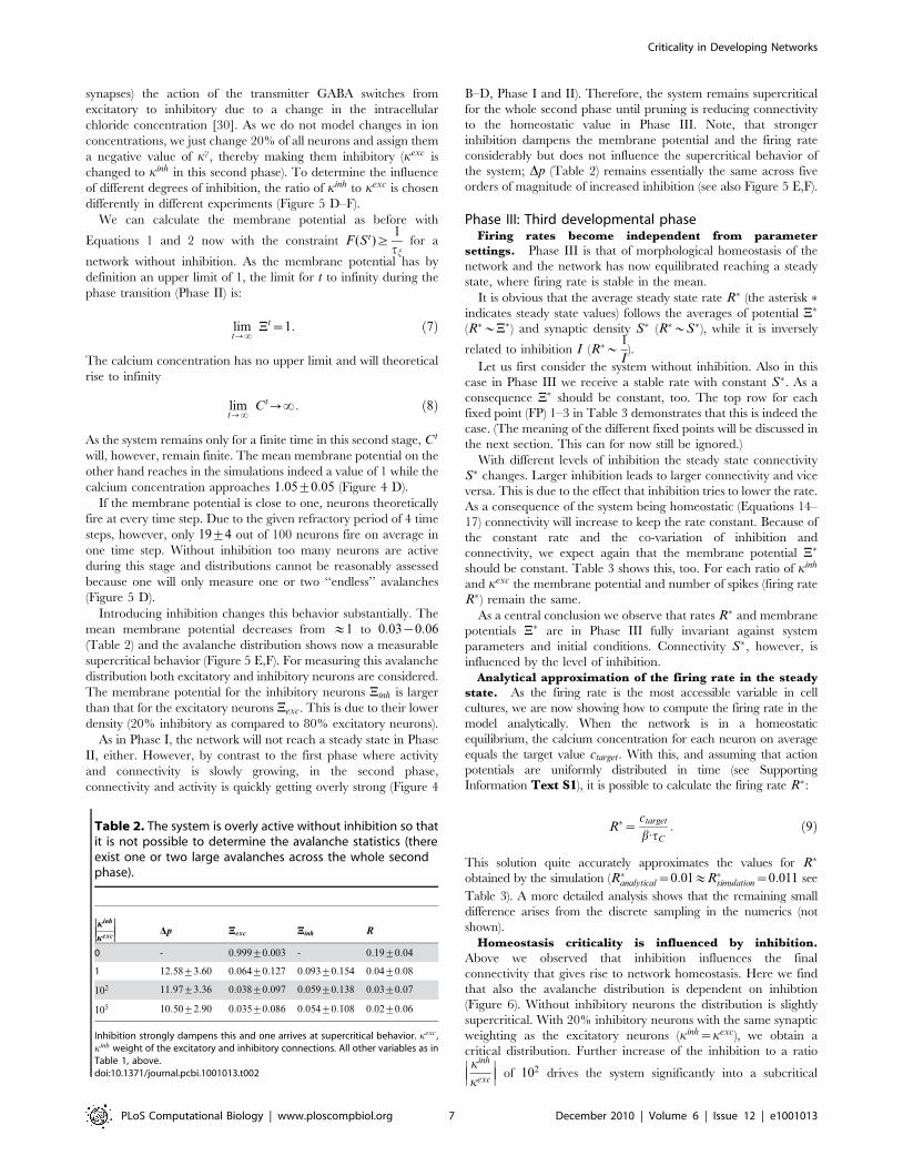
(Figure 6). Without inhibitory neurons the distribution is slightly

supercritical. With 20% inhibitory neurons with the same synaptic

weighting as the excitatory neurons (kinh~kexc), we obtain a

critical distribution. Further increase of the inhibition to a ratio

Dkinh

kexcD of 102 drives the system significantly into a subcritical

Table 2. The system is overly active without inhibition so thatit is not possible to determine the avalanche statistics (thereexist one or two large avalanches across the whole secondphase).

Dkinh

kexcD Dp Jexc Jinh R

0 - 0:999+0:003 - 0:19+0:04

1 12:58+3:60 0:064+0:127 0:093+0:154 0:04+0:08

102 11:97+3:36 0:038+0:097 0:059+0:138 0:03+0:07

105 10:50+2:90 0:035+0:086 0:054+0:108 0:02+0:06

Inhibition strongly dampens this and one arrives at supercritical behavior. kexc ,kinh weight of the excitatory and inhibitory connections. All other variables as inTable 1, above.doi:10.1371/journal.pcbi.1001013.t002



regime. A further increase to 105 does not significantly increase

subcriticality anymore.

This demonstrates that criticality after equilibration, hence on

the long run, depends on connectivity but neither on the mean

membrane potential J� nor on the resulting average firing rate R�.Criticality is subject to acute changes in inhibition. This

can be nicely demonstrated by disturbing an equilibrated system

by a sudden change of inhibition (Figure 7). After such a jump,

connectivity S (and, thus, criticality, see Figure 7) changes, but

mean membrane potential J and rate R will relax back to their

previous values. This long term process is initiated by the activity

change that follows the artificially induced change of inhibition.

Panels C and D in Figure 7 show that immediately after the jump,

criticality changes to relatively high(low) values for Dp for the

super(sub)-critical case (left vs right columns in Figure 7). A similar

experiment has been performed by Beggs and Plenz [1] (see inset

in Figure 7 A) where reduced inhibition also led to a supercritical

system. While in our system activity fully builds back, super(sub)-

criticality does not.

A comparison between panel B in Figure 6, which represents

the fully relaxed case, with panels C and D in Figure 7, which

represent the situation immediately after the jump, shows this

clearly. Hence, while the activity change leads to an immediate

change in criticality, it is the lasting change of connectivity that

leads to the fact that also the changed criticality persists albeit on a

reduced level.

Thus, the model predicts that sudden activity changes should

affect criticality in Phase III, but in a reversible way. Lasting

changes of inhibition, on the other hand, should also lead to lasting

small changes in the criticality without affecting the mean firing rate

in the network.

Dynamic network behaviour: Isoclines and fixed pointsSo far we have described the three development phases for our

network model showing how criticality depends on network state,

where the final state suggests some kind of fixed point behavior. In

the following we will assess to what degree this process is

characteristic for the system. To this end, we calculate its nullclines

analytically [24] and compare these results with the simulations in

Figure 8. For simplicity here we treat only a purely excitatory

network.

To be able to solve the problem analytically we assume that the

change of the connectivity stij between neurons and their

membrane potential jti is slow and derivatives can, thus, be set

to zero. Furthermore, on longer time scales the differences

between neurons are negligible and only the behavior of the

means need to be considered. As a result one can calculate the

nullcline of this system (see Supporting Material Text S2), which

describes a hysteresis curve (Figure 8 A):

St~Jt{j0

tjkexcG(Jt)ð10Þ

St and Jt are the mean values of stij and jt

i over all neurons. G(Jt)

is a sigmoidal function as an approximation for the Heaviside

function H, which determines when an action potential is

generated (see Supporting Material Text S2). In Figure 8 A we

also plot the trajectories which belongs to this system and the other

(trivial) nullcline Jt~const:, which describes the fact that the

system develops into homeostasis. At fixed point F development

stops. In Figure 8 B we plot the actual development of St and Jt

observed in the simulations. Ideally this curve should match one of

the trajectories in panel A and one can see that this is essentially

the case. The main deviation arises from the fact that, due to the

required simplifications, the analytical solution in panel A shows

during the phase transition (Phase II) infinite growth and this

cannot be achieved in the simulation. This leads to a reduction in

the rising slope of panel B and to the fact that the fixed point F is

shifted closer to the inflexion point of the isocline.

When considering axons and dendrites separately, fixed point Fsplits into a zone of many points, which correspond to the same

connectivity S�, and hence lie on a hyperbola in Figure 8 C

(dashed line). These fixed points form an omega-limit set in phase

space and are represented by the equilibrium point F in the S-J-

space. The approximate path of a trajectory from panels A and B

is shown in Figure 8 C by the solid white line. Above we had stated

that rates R� and membrane potentials J� are in Phase III fully

invariant against system parameters and initial conditions, while

Table 3. In the homeostatic state (Phase III), the membrane potential J� is independent of the attained fixed point (FP) and theinhibition (ratio of kinh to kexc).

FP Dkinh

kexcD Dp J�exc J�inh R� S�:10{6

1 0 0:199+0:015 0:015+0:014 - 0:011+0:014 2:39+0:018

1 {0:070+0:025 0:015+0:017 0:015+0:017 0:011+0:014 4:15+0:032

102 {0:801+0:019 0:015+0:017 0:015+0:017 0:011+0:014 6:47+0:045

105 {0:771+0:019 0:015+0:017 0:015+0:017 0:011+0:014 6:43+0:044

2 0 0:037+0:040 0:015+0:014 - 0:011+0:014 2:40+0:018

1 {0:038+0:025 0:015+0:017 0:015+0:017 0:011+0:014 4:08+0:031

102 {0:812+0:022 0:015+0:017 0:015+0:017 0:011+0:014 6:33+0:047

105 {0:735+0:014 0:015+0:017 0:015+0:017 0:011+0:014 6:53+0:047

3 0 0:170+0:02 0:015+0:014 - 0:011+0:014 2:39+0:019

1 0:009+0:010 0:015+0:017 0:015+0:017 0:011+0:014 4:14+0:032

102 {0:709+0:018 0:015+0:017 0:015+0:017 0:011+0:014 6:56+0:045

105 {0:803+0:032 0:015+0:017 0:015+0:017 0:011+0:014 6:29+0:045

By contrast, connectivity S� and the avalanche distribution Dp changes with the level of inhibition.doi:10.1371/journal.pcbi.1001013.t003



connectivity S� is influenced by the level of inhibition. To this we

can now add that the actual balance between axonal supply A�

and dendritic acceptance D� (location of the different fixed points)

remains dependent on the initial conditions (as well as on the

inhibition) and should, therefore, be the most sensitive develop-

mental parameter, e.g. much susceptible to pharmacological

interference.

Furthermore, as the rate essentially follows S� and J� and

inversely I , we can state that the isocline in Figure 8 A will, for

larger inhibition, be shifted diagonally upwards away from the

origin shifting the fixed point to a higher synaptic density.

The dynamic behavior shown in Figure 8 is similar to that

observed in the studies of Van Ooyen and Van Pelt [24] and our

results show that the three development phases (Phase I, II and III)

of this system are generic and independent of the chosen simulation

parameters and confirm the existence of a strong phase transition.

Comparison between cell culture and modeldevelopment

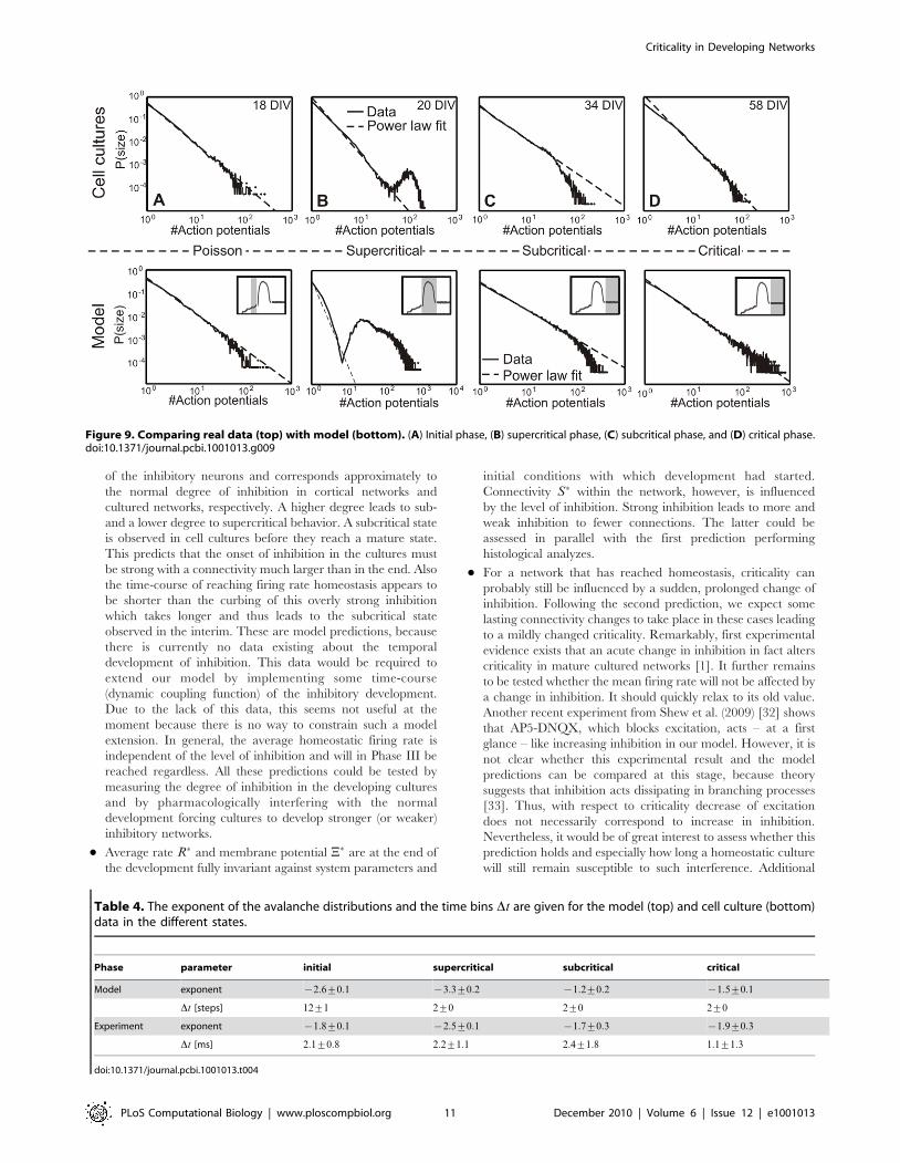
Figure 9 shows a comparison of the different criticality states

between cell culture (top) and model data (bottom) summarizing

some of the observations from above. Additionally, the exponent

of the avalanche distribution and the time bins Dt are given in

Table 4 for each state in model and cell cultures. In the model, at

the end of the transition from Poisson to power law (Figure 5 C),

little connectivity in Phase I leads to an initial state similar to that

observable in dissociated cell cultures (Figure 9 A). This is followed

by strongly rising synaptic density in Phase II (B). Accompanying

the overshoot in network activity and connectivity, the model

network passes a transient phase of supercriticality (B, bottom) as

do the cell cultures (B, top). Depending on the chosen strength of

inhibition, we obtain in Phase III a subcritical state for the model

(C, bottom,kinh

kexc~102) similar to that in cell culture data (C, top).

Thereafter, still in Phase III, we have gradually reduced the

inhibitory strength to kinh~kexc, hence balancing synaptic strength

for inhibition and excitation (while keeping the number of inhibitory

neurons constant). This leads to a final critical state in the model (D,

bottom) similar to that found in cell culture data (D, top).

Thus, this predicts that that developing inhibition is an important

factor for the course of criticality in developing neuronal networks.

Only if inhibition in the model is lowered in Phase III again, the

network becomes critical. Therefore, it is likely that overall synaptic

pruning in developing networks not only affects excitatory but also

inhibitory synapses [31]. Moreover, neuronal networks seem to

reach firing rate homeostasis earlier than the equilibrium for

maturing inhibition (compare discussion in Figure 7).

Additional inter-spike interval (ISI) and cross-correlation (CC)

analyzes have been performed. ISIs and CCs are very similar

between cultures and model across all stages but they do not

contain interesting features (like oscillations) and therefore we do

not show these diagrams here to save some space.

Predictions of the modelThe following predictions are derived from the model:

N Criticality at the end of development is optimally reached with

20% inhibition with a strength equal to that of the excitation.

This observation does not depend crucially on the distribution

Figure 6. In the homeostatic equilibrium (Phase III), the degree of inhibition determines whether the network finally reaches acritical state or remains sub- or supercritical. As a characteristic example the avalanche distributions from fixed point 1 (see Table 3) are shown.(A) A purely excitatory network stays slightly supercritical although network activities are homeostatically balanced (Dp~0:199+0:015). (B) If theabsolute value of the inhibitory strength kinh equals the excitatory strength kexc the network becomes critical (Dp~{0:070+0:025). Here the totalnumber of inhibitory synapses is about 20%. (C–D) Higher levels of inhibition (102 for C and 105 for D) keep the network in a subcritical regime (C:Dp~{0:801+0:019; D: Dp~{0:771+0:019).doi:10.1371/journal.pcbi.1001013.g006



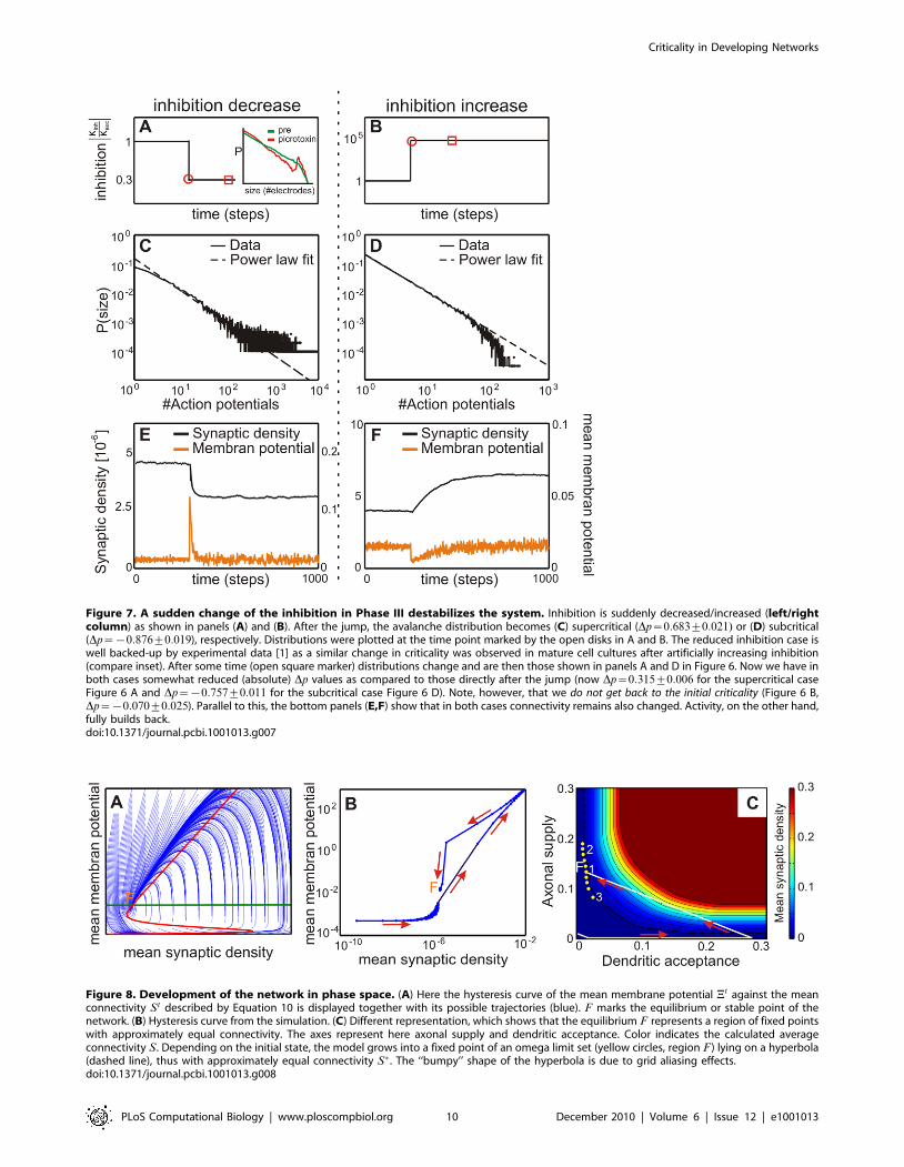
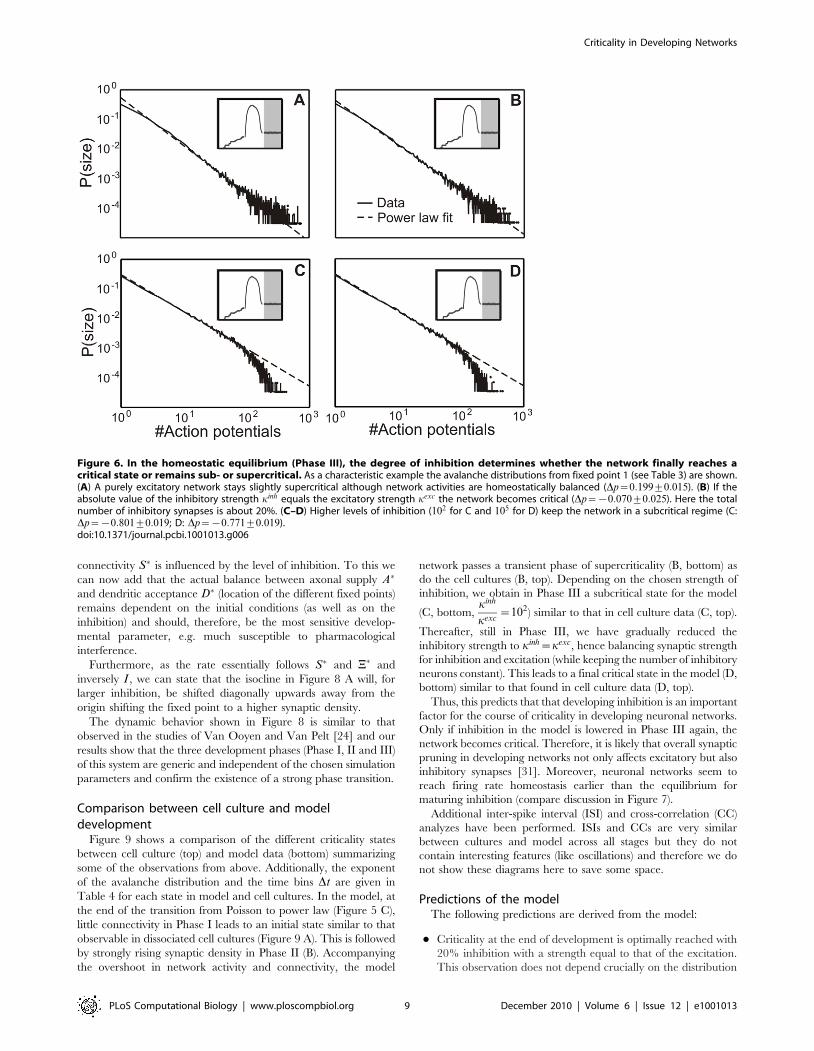
Figure 7. A sudden change of the inhibition in Phase III destabilizes the system. Inhibition is suddenly decreased/increased (left/rightcolumn) as shown in panels (A) and (B). After the jump, the avalanche distribution becomes (C) supercritical (Dp~0:683+0:021) or (D) subcritical(Dp~{0:876+0:019), respectively. Distributions were plotted at the time point marked by the open disks in A and B. The reduced inhibition case iswell backed-up by experimental data [1] as a similar change in criticality was observed in mature cell cultures after artificially increasing inhibition(compare inset). After some time (open square marker) distributions change and are then those shown in panels A and D in Figure 6. Now we have inboth cases somewhat reduced (absolute) Dp values as compared to those directly after the jump (now Dp~0:315+0:006 for the supercritical caseFigure 6 A and Dp~{0:757+0:011 for the subcritical case Figure 6 D). Note, however, that we do not get back to the initial criticality (Figure 6 B,Dp~{0:070+0:025). Parallel to this, the bottom panels (E,F) show that in both cases connectivity remains also changed. Activity, on the other hand,fully builds back.doi:10.1371/journal.pcbi.1001013.g007

Figure 8. Development of the network in phase space. (A) Here the hysteresis curve of the mean membrane potential Jt against the meanconnectivity St described by Equation 10 is displayed together with its possible trajectories (blue). F marks the equilibrium or stable point of thenetwork. (B) Hysteresis curve from the simulation. (C) Different representation, which shows that the equilibrium F represents a region of fixed pointswith approximately equal connectivity. The axes represent here axonal supply and dendritic acceptance. Color indicates the calculated averageconnectivity S. Depending on the initial state, the model grows into a fixed point of an omega limit set (yellow circles, region F ) lying on a hyperbola(dashed line), thus with approximately equal connectivity S� . The ‘‘bumpy’’ shape of the hyperbola is due to grid aliasing effects.doi:10.1371/journal.pcbi.1001013.g008



of the inhibitory neurons and corresponds approximately to

the normal degree of inhibition in cortical networks and

cultured networks, respectively. A higher degree leads to sub-

and a lower degree to supercritical behavior. A subcritical state

is observed in cell cultures before they reach a mature state.

This predicts that the onset of inhibition in the cultures must

be strong with a connectivity much larger than in the end. Also

the time-course of reaching firing rate homeostasis appears to

be shorter than the curbing of this overly strong inhibition

which takes longer and thus leads to the subcritical state

observed in the interim. These are model predictions, because

there is currently no data existing about the temporal

development of inhibition. This data would be required to

extend our model by implementing some time-course

(dynamic coupling function) of the inhibitory development.

Due to the lack of this data, this seems not useful at the

moment because there is no way to constrain such a model

extension. In general, the average homeostatic firing rate is

independent of the level of inhibition and will in Phase III be

reached regardless. All these predictions could be tested by

measuring the degree of inhibition in the developing cultures

and by pharmacologically interfering with the normal

development forcing cultures to develop stronger (or weaker)

inhibitory networks.

N Average rate R� and membrane potential J� are at the end of

the development fully invariant against system parameters and

initial conditions with which development had started.

Connectivity S� within the network, however, is influenced

by the level of inhibition. Strong inhibition leads to more and

weak inhibition to fewer connections. The latter could be

assessed in parallel with the first prediction performing

histological analyzes.

N For a network that has reached homeostasis, criticality can

probably still be influenced by a sudden, prolonged change of

inhibition. Following the second prediction, we expect some

lasting connectivity changes to take place in these cases leading

to a mildly changed criticality. Remarkably, first experimental

evidence exists that an acute change in inhibition in fact alters

criticality in mature cultured networks [1]. It further remains

to be tested whether the mean firing rate will not be affected by

a change in inhibition. It should quickly relax to its old value.

Another recent experiment from Shew et al. (2009) [32] shows

that AP5-DNQX, which blocks excitation, acts – at a first

glance – like increasing inhibition in our model. However, it is

not clear whether this experimental result and the model

predictions can be compared at this stage, because theory

suggests that inhibition acts dissipating in branching processes

[33]. Thus, with respect to criticality decrease of excitation

does not necessarily correspond to increase in inhibition.

Nevertheless, it would be of great interest to assess whether this

prediction holds and especially how long a homeostatic culture

will still remain susceptible to such interference. Additional

Figure 9. Comparing real data (top) with model (bottom). (A) Initial phase, (B) supercritical phase, (C) subcritical phase, and (D) critical phase.doi:10.1371/journal.pcbi.1001013.g009

Table 4. The exponent of the avalanche distributions and the time bins Dt are given for the model (top) and cell culture (bottom)data in the different states.

Phase parameter initial supercritical subcritical critical

Model exponent {2:6+0:1 {3:3+0:2 {1:2+0:2 {1:5+0:1

Dt [steps] 12+1 2+0 2+0 2+0

Experiment exponent {1:8+0:1 {2:5+0:1 {1:7+0:3 {1:9+0:3

Dt [ms] 2:1+0:8 2:2+1:1 2:4+1:8 1:1+1:3

doi:10.1371/journal.pcbi.1001013.t004



long term mechanisms, not captured by our model, might in

reality terminate this effect after some time.

N The model further predicts that the actual balance between

axonal supply A� and dendritic acceptance D� is quite

sensitively depending on the initial conditions under which a

cell culture starts its individual development. Thus, any

histological analysis of connectivity S� should best be

performed by carefully assessing dendritic and axonal

parameters in the different cultures. Even with very similar

initial conditions, we expect those to vary widely across

cultures, while the total connectivity S� should be very similar.

In this study this is reflected in the behavior of the PKC

(Protein Kinase C)-inhibited cultures, which do not show any

visible differences in their avalanche and firing rate charac-

teristics as compared to non-treated cultures. The PKC-

inhibited cultures express much richer dendritic structures

[34–36]. However, the lack of difference in activity patterns

found here suggests that the final synaptic density in these

cultures does not substantially differ from that in the controls.

The model predicts that this should go hand in hand with a

shift of the fixed point along the hyperbola in Figure 8 C,

which, however, does not alter the found avalanches. The

prediction of a fix-point shift could be tested by detailed and

complex histological analyzes of the existing synapses in

controls and PKC-inhibited cultures, which goes beyond the

scope of this study.

These predictions are quite specific as they do not depend on

the parameter choices in the model, which is one strength of this

approach. Most predictions, if not all, can be tested in a straight

forward way in future experiments, albeit requiring substantial and

sometimes difficult experimental work which can only be

addressed in future work.

Discussion

In the current study we have investigated how the activity

patterns in developing cell cultures can be measured and modeled

in terms of self-organized criticality. We have shown that the

activity distributions in real cultures undergo a transition from a

stage with little activity to a supercritical and then a subcritical

state and finally to critical behavior. These transitions were

significant for the cell cultures analyzed.

We used an extended version of the neurite outgrowth model by

Van Ooyen and co-workers [10,24,25] with separate axonal and

dendritic fields. The axonal and dendritic growth is driven by the

goal to reach firing rate homeostasis as modeled in previous papers

by Butz and co-workers [26,27]. The model was able to reproduce

the different developmental phases and several interesting

predictions have been made.

Relating criticality to morphological developmentIn general the chosen abstractions in the model appear to match

the data description level quite well, but the question arises to what

degree this still corresponds to reality in developing networks.

Most importantly, the network stages described above must be

related to the morphological development of dissociated neurons

and their growing connectivity in culture which determines the

activity pattern at every point in time [37–39].

It is well known [40] that the development of connectivity in

cultures follows several phases. An initial phase (Phase I) is

characterized by neuritic growth, followed (Phase II) by a

structural overshoot and pruning followed by a maturation phase

(Phase III) which finally leads to stable mean connectivity. Slowly

growing connectivity in Phase I [41] leads over to the fast building

of many synapses and a strong increase in activity in Phase II

[38,42], while pruning leads to Phase III with reduced number of

synapses and lower activity [37]. Thereafter, firing behavior

remains unchanged for two months [38,42]. One may conclude

that when synaptic pruning ceases, connectivity becomes stable

and neuronal activities turn into homeostasis. Stable connectivity

means that the sum of existing synapses does not vary much in

time. The topology of the network can, however, not be predicted

by the model as for this purpose a more detailed model of axons

and dendrites would be required. However, neuronal development

towards homeostasis substantially accelerates by increasing

neuronal activities due to disinhibition by picrotoxin, a GABAer-

gic synapse blocker [43]. Considering other transmitter studies,

neuronal activity via increased glutamate release is likely to

promote axonal outgrowth [44,45] and therefore leads to a faster

synapse formation and to an earlier maturation of the cell culture.

Importantly, the behavior of dissociated neurons forming networks

spontaneously occurs in any cell culture regardless of the original

source of the plated neurons like cortex or hippocampus [46].

While certain simplifying assumptions had to be made to arrive

at the basic differential equations (Equations 14–17) of our model,

these experimental results clearly support the general dynamics

assumed for our model.

In our model, networks with about 20% inhibition where the

only ones that reached a robust critical state. While this level of

inhibition corresponds to that in real nets, the results is intriguing

as homeostasis of the firing rate will also be reached with much

different levels of inhibitory cells. As known from literature

[47,48], GABA changes during the development from an

excitatory to an inhibitory transmitter. As this is a fast process,

inhibition sets in rapidly in the overshoot Phase II [48,49] and

possibly with a too high level. As discussed above, the observed

subcritical phase clearly suggests a pruning phase for the inhibition

which lasts longer than the firing rate equilibration. An indication

of the functional role of synaptic pruning of inhibitory synapses

was recently obtained from the developing auditory system in

gerbils [31].

Like others [24,25,50,51], also our model assumes that the main

determining force within a growing network is the attempt of the

neurons to achieve on average activity homeostasis. Several

existing studies indicate that neurons, which are too active, seek to

reduce their firing [50,52], whereas neurons that are too quiescent

try to increase it [53,54]. Activity reduction is achieved by a

reduction of the inputs to the cell (for example dendritic

withdrawal) and vice versa. At the same time, highly activated

cells respond with axonal outgrowth [44,45,55,56] as increased

levels of intracellular calcium, as a second messenger, regulates

growth cone motility and therefore affects neurite outgrowth

[44,56–60].

Self-organized criticality in neuronal networksSelf-organized criticality represents the situation that many

systems of interconnected, nonlinear elements evolve over time

into a critical state in which the probability distribution of

avalanche sizes can be characterized by a power law. This process

of evolution takes place without any external instructive signal. As

analytically shown [7], an important feature of the power law is its

scale invariance. This means that all neuronal avalanches

regardless of their size (number of spikes) can be treated as

physically equal [3]. Furthermore, avalanches remain stable in

their spatial and temporal configuration for many hours, as

already shown in cortical slices [15]. So, avalanches have optimal

preconditions (equality and stability) to be a candidate for memory



patterns. The stability of these effects is strongly supported by the

way our model systems develop as will be discussed next.

The current study shows that networks in cell cultures undergo

a certain transition during their morphological development.

Thus, this paper is in the tradition of a sequence of investigations

[17,40,43,45] that try to link cell culture activity and development

to possible in vivo stages. Indications exist indeed that different

activity states in cultures could be matched to in vivo states [61],

but one needs to clearly state that culture and in vivo development

also show clear differences. In vivo development is much more

structured which will lead to differences in (ongoing) activity. As

discussed above, dendritic and axonal fine structure and their

spatial distribution, however, does not seem to critically affect the

observed state-transitions. Hence, this supports that, at the level of

avalanches, little difference might indeed exist between culture and

in vivo. A study by Stewart and Plenz [21] suggests that avalanche

frequency is correlated to the integrated amplitude of local field

potentials, which grows until 25 DIV in their study. This indicates

that also their networks had developed from a low-activity state

into states that follow a power-law distribution. They show that

distributions have in general an exponent of 21.5, indicative of a

branching parameter of 1 [1], and a closer look at their result

suggests that transitory (sub- and supercritical) stages are also

observable in this data set (see, e.g., Fig. 3D in Stewart and Plenz

2008 [21]). A related study by Pasquale et al. [17] confirms this

observation. It, thus, seems that the critical state represents the

final state of the development, which – in the model – is reached

together with firing rate homeostasis. This leads to a high degree of

stability, which would be desirable also from a functional

viewpoint. This is supported by the observation that in Phase III

in the model sudden changes of the network structure (e.g. by a

sudden change of inhibition) will only lead transiently to a stronger

disruption of criticality. Indeed, the system soon find its way back

into homeostasis and criticality is only little affected.

Several previous studies [1,17,21,32] focused on the exponent of

the power law in the critical state. This is a characteristic

parameter of the system and found to be around {1:5[1,17,21,32]. We find that the exponent is {1:50+0:07 in

simulations and {1:90+0:3 in cell cultures. Thus, the exponent

matches previous results very well for the simulations. The

difference in the experiments from the theoretical value of {1:5can occur from variations in the time bin, too harsh selection

criteria, or a too small number of data points. Thus, deviations

leading to the found value of {1:9 fall into the tolerance range of

these experiments. In addition, it is not clear if the theoretical

value of {1:5 gained from branching processes [62] can be

applied to all self-organizing systems in the critical state (f.e. Bak et

al., 1987 [6]). Hence, it is equally well possible that the activity of

the cultures is critical but does not exactly follow a branching

process.

In a previous study Beggs and Plenz [1] have shown, that the

critical state is optimal for a neuronal system concerning

information flow. If the system is subcritical information will die

out. The opposite situation is an epileptic system with too many

long avalanches (supercritical state). Thus, a neuronal network in

the critical state has the maximal dynamical range to react to

incoming (external) information arriving from complex interac-

tions of the neural system with its environment. The experimental

part of the current study shows that real networks will develop

towards such a state and the model suggests that this state is rather

stable and therefore computationally reliable. Follow-up investi-

gations, hopefully triggered by this research, might shed a light on

the structural and functional dynamics of self-organized criticality

in real developing brains and possibly also contribute a better

understanding of developmental pathologies.

Methods

Experimental approach and data evaluationPreparation of the cell cultures. Primary cortical cell

cultures were prepared as described previously [63,64]. Cells

were derived from cortices of neonatal wistar rats by mechanical

(chopping with scalpel, trituration) and enzymatical (0.05%,

Trypsin, 15min at 370C.) dissociation and plated at densities

(CASY cell counter, Innovatis) of 500,000 cells per cm2 onto

polyethyleneimine-coated micro-electrode arrays (59 TiN

electrodes, 200/500mm electrode pitch, Multi Channel Systems).

Cultures developed in 1ml growth medium, minimum essential

medium (Gibco) supplemented with heat-inactivated horse serum

(5%), L-glutamine (0.5mM), glucose (20mM) and gentamycin

(10mg/ml). One third of medium was exchanged twice per week.

Cultures were maintained at 5% CO2 and 370C. In a subset of

cultures PKC (Protein Kinase C) was chronically inhibited by

addition of a PKC antagonist (Go6976, 1 mM, Calbiochem) at the

first exchange of the culture medium at 1 DIV. This different

treatment has no significant influence on different parameters of

the cell cultures (see Table 5) and, therefore, on the results of this

paper.

Electrophysiology. Electrophysiological recordings were

performed on the different DIVs at the same time for one hour

under culture conditions with a MEA1060-BC system amplifier

(Multi Channel Systems) [65]. Raw electrode signals were digitally

high-pass filtered at 200Hz and action potentials were detected by

voltage threshold (3 times of standard deviation from the mean)

using MC-Rack software (Multi Channel Systems).

Selection criteria. Clustering of neurons [66] at few

electrodes can distort the avalanche statistics as clustering is a

culture phenomenon and not seen in-vivo. To avoid clustering

induced effects, we demand that activity has to be nearly uniformly

distributed across all electrodes. So, all electrodes are excluded

from the statistics which have measured more activity than two

times the standard deviation from the mean activity per electrode.

As shown in the literature [1,3,17] a too small number of

measuring electrodes distorts the avalanche distribution (fewer

Table 5. Cell cultures with PKC and without PKC (untreated) are compared.

Dp exponent Dt [ms]AP

min

std(act:)

mean(act:)act. elec.

Untreated {0:16+1:16 {1:94+0:39 4:06+4:32 1343+1067 1:47+0:58 55+2

PKC {0:49+0:47 {1:77+0:24 2:12+3:09 1219+706 0:98+0:41 55+3

There are no significant differences. For the mean activity per minute the supercritical states are excluded as this state is too active leading to an unwanted bias in thedata. For definition of the variables see the remainder of this Method section.doi:10.1371/journal.pcbi.1001013.t005



long avalanches) and decreases classification of different states.

This is avoided by choosing only samples with at least 50 active

electrodes.

A total of 40 cultures has been originally considered in this

study. Of the 40 cultures 22 were controls and 18 were PKC

inhibited. A total of 20 cultures did not obey the tight prior

selection criteria for allowing rigorous criticality analysis and had

to be excluded. The final number of analyzed cultures was, thus,

12 controls and 8 PKC inhibited. This shows that both groups

were equally affected by the selection criteria. Interestingly, and

also predicted by the model (see ‘‘Predictions of the Model’’), no

differences with respect to the activity analyzes of the current study

were found between controls and PKC-inhibited cultures. Thus

results were pooled.

Definition of avalanches. order to assess the distribution of

avalanches in cell cultures and in the model in the same manner,

we search for the beginning and the end of an avalanche by a

gliding time bin of a fixed size. Whenever the system is silent (no

spikes) for at least the duration of the time bin, an avalanche ends

and a new one starts with the next spike. The time bin is the mean

time interval between two spikes in the system. Too long time

intervals are sorted out by first calculating the mean cross-

correlation of all electrode signals and secondly by getting the time

value for which 99% of the integration area is under this mean

cross-correlation curve. This time value is the maximum time

interval which is taken into account of the mean time interval [1].

This way we ensure that bursts on a longer timescales do not

distort the statistics. This definition of avalanches can be used for

cell culture and model data.

Measuring the deviation from a power law. To

distinguish between the different states of an SOC system, the

measure Dp is defined. For this, the theoretical power law

distribution ptheo is calculated by a linear regression of the linear

start on the left side (at approximately 100) of the distribution porig

in the log-log-plot with MATLAB to the end of the linear

behaviour. Now, for each data point x the regression ptheox is

subtracted from porigx . The mean of the differences of all data

points is the measure Dp.

Dp~X

x

porigx {ptheo

x ð11Þ

We define the following relation between Dp and the state of the

system:

Dpv{0:195 < subcritical

Dp[({0:195,0:195) < critical

Dpw0:195 < supercritical

These thresholds are heuristic as there is no theoretical

background for this. In general they correspond well to state

classification if made by human inspection. Note, the results of this

paper are not crucial dependent on narrow threshold margins.

Additional tests for criticality and data evaluation.

Measuring a power law for the avalanche distribution is not

sufficient to conclusively show that a system is in the critical state,

because a power law can also result from the summation of two

exponentials [7]. Therefore, the critical state in model and cell

cultures has to be analysed by additional tests showing the scale-

free behavior. Several tests were performed and results are shown

here. First, the avalanche distribution has to show a power law

even with less neurons (model) or electrodes (cell culture),

indicating that the system is spatially scale-free. Figure 10 A,B

demonstrates this. Furthermore, a system in the critical state has

also to be temporally scale-free. To show this, different time bins are

used for analyzing the avalanche distribution. Also these

distributions show a power law relation (Figure 10 C,D) for

model and cell cultures.

A third informative test is to assess the scale-free behavior of the

inter-avalanche intervals (g). For this a minimum event size s has

to be introduced (minimum number of spikes in one avalanche)

and then the time interval g between the occurrence of two

avalanches larger as s can be measured. Thus, for all values of gthe probability distribution D(g,s) of getting an inter-avalanche

interval g given s is assessed and can be re-scaled by the rate R(s)of having an avalanche larger than s per time unit (g?gR(s),D(g,s)?D(g,s)=R(s)). If this is done for different s and all

distributions form a single curve, the system is scale-free and the

curve is the scaling function [67].

D(g,s)~R(s): (gR(s)) ð12Þ

This is done for our model and cell cultures in the critical state

(Figure 10 E,F). Note, the actual shape of the different scaling

functions is of less importance. The scale-free property is confirmed

as long as all functions for a given system collapse onto the same

function [67]. This is indeed observed in Figure 10 E,F.

Finally, a fourth test for criticality is the Fano Factor [68–70],

for which the number of spikes N(t,tzT) in a time window from tto tzT has to be considered using following equation

F (T)~vN2(t,tzT)w{vN(t,tzT)w2

vN(t,tzT)wð13Þ

The Fano Factor F (T) assumes a point process of events (spikes)

and relates the clustering of these events to a Poisson process for

which F (T)~1. When the Fano Factor is below one, it indicates

that the point process is more orderly than a Poisson process, and

a Fano Factor above one indicates increased clustering at the given

time scale T [69]. For a scale-free point process (e.g.; a system in

the critical state), the Fano Factor needs to be a power law with the

form TaF . The exponent is an approximation of the 1=f exponent

which is related to the exponent of the avalanche distribution [9].

For the critical state in our model and cell cultures the Fano

Factor shows a power law behavior for a wide range of time

windows T (Figure 10 G,H). There are no large differences

between model and cell culture exponents (0:76+0:03 for model

and 0:78+0:03 for cell cultures). Only at large values of T , around

102 steps or 102 ms, model and cell culture data do not show a

power law behavior anymore and start to differ. However, the

important range for the avalanche analysis is at smaller T -values

(compare time bin Dt in Figure 10 G,H and Table 4).

Computational modelling approachIn order to investigate the relationship between network

development and self-organized criticality, we extended the

previous neurite outgrowth model by Van Ooyen and Van Pelt

[10,24,25] by separate axons and dendrites. The model is

essentially a two-dimensional recurrent neuronal network with

uni-directional synapses. Model neurons are described by four

equations; for activity j, internal calcium concentration c as well as



dendritic acceptance d, and axonal supply a. The last two

parameters determine the connectivity s which is a generalisation

of synaptic weights and the number of synapses between neurons.

In line with previous experimental [27,45,50] and modelling

studies [23,24,71,72], the processes which determine the dynamics

of this system can be summarized very briefly as: The activity of

each neuron affects its calcium concentration. This, in turn,

specifies the change of the dendritic and axonal offers, hence, the

Figure 10. Additional tests for criticality used for cell cultures and model. In (A,B) we address potential spatial non-stationarity effects bycomparing distributions obtained with only certain percentage subsets of the electrodes (neurons). In (C,D) we show that only minor variations existfor different time bins. Thus, temporal non-stationarities on a short time scale appear unlikely. Panels (E,F) show the scaling function F and,therefore, the scale-free behavior of model and cell cultures. Panels (G,H) show a Fano factor analysis for cell culture and model in the critical state.The exponent of the Fano Factor (linear regression) is 0:76+0:03 for the model and 0:78+0:03 for cell cultures. Hence we conclude a scale-freeclustering over different time scales T .doi:10.1371/journal.pcbi.1001013.g010



connectivity which will then gradually influence activity and so on.

In the following we define parameters and equations. These

equations are solved by the Euler method with an interval length

of one simulated time step.Membrane potential. As in the main text in the following,

mean values are given as upper case letters, while lower case letters

indicate individual values. For a fixed connectivity, given by the

synaptic density between dendritic and axonal offers, each neuron

has a certain activity. In accordance to the definition of the neuron

model in the work by Abbott and Rohrkemper [10], the activity of

the i-th neuron at the time point t is given by a membrane

potential jti , limited by a hard bound to 1, which decays in time

exponentially with time constant tj to j0, where j0 is the resting

membrane potential. jti increases proportionally to the

connectivity stij if a neighboring neuron j generates an action

potential (jtjw%t

j ; %tj is a uniformly distributed number between 0

and 1. This relation between jtj and %t

j is obtained by the

Heaviside-function H).

djti

dt~

j0{jti

tjzXN

j~1

kcj st

ij H jtj{%t

j

� �: ð14Þ

kc defines if a presynaptic neuron is inhibitory (kinhv0) or

excitatory (kexcw0). In the beginning of the simulation, all

neurons are excitatory comparable to the very early development

of biological neuronal networks [48]. At some point during

simulation, a certain subset of neurons (20% of all) is converted

into inhibitory neurons (see subsection Phase II of the Results

section). We further define a refractory period of four time steps.Calcium concentration. We model the calcium dynamics in

our neuron model related to the work by Abbott and Rohrkemper

[10]. The membrane potential jti affects the calcium concentration

cti which has a slower exponential time constant tC . If a neuron i is

active, it receives an influx of calcium and the concentration

increases by b.

dcti

dt~{

cti

tC

zb H jti{%t

i

� �: ð15Þ

cti determines the change of the synaptic density st

ij .

Dendritic acceptance, axonal supply and connectivity.

The development of dendrites and axons depends indirectly, by

ways of the calcium concentration, on the activity. Lipton and

Kater [45] showed that the deviation of the calcium concentration

of a neuron from a certain target value determines its outgrowth.

In line with previous modelling studies [10,23,24,72], we defined a

homeostatic value ctarget for which the axonal and dendritic offers

(and with them the synaptic density) remains unchanged if cti

equals ctarget. The rules for growth and retraction of continuous

axonal supply and dendritic acceptance were taken from the

modelling approach by Dammasch and Butz [23,73] and can be

described as follows: If the neuron has a too high membrane

potential jti , hence a too high calcium concentration ct

i , the

dendritic acceptance dti shrinks proportionally to a constant cden

leading to a decrease of its input. If the membrane potential is too

low, the dendritic acceptance increases to receive more inputs

raising the calcium concentration by an increasing membrane

potential to the homeostatic value. The axonal supply ati behaves

equally but with inverted sign and different growth rate caxo.

ddti

dt~{cden (ct

i{ctarget) ð16Þ

dati

dt~ caxo (ct

i{ctarget): ð17Þ

Finally, we define the connectivity between neurons i and j by:

stij~Ct

1:at2

j {1

2at2

j sin 2:Ct1

� �zCt

2:dt2

i {1

2dt2

i sin 2:Ct2

� �ð18Þ

with

Ct1~ arccos

at2

j zf2ij{dt2

i

2atjfij

!

Ct2~ arccos

dt2

i zf2ij{at2

j

2dti fij

!

and fij as distance between neuron i and j. This essentially

represents the overlap of the axonal and dendritic probability

zones which can be understood as an abstract representation for

the probability of synapse formation. In the simulations the

neurons are distributed on a open grid to avoid developmental

unsteadinesses followed from irregularities in the neuronal density.

However, the overall behavior is not effected by this.

Parameter settings. The following table (Table 6) shows all

standard parameter values. Exceptions are indicated in the text.

Supporting Information

Text S1 Derivation of the steady state firing rate R*.

Found at: doi:10.1371/journal.pcbi.1001013.s001 (0.03 MB PDF)

Text S2 Derivation of the nullcline of the model.

Found at: doi:10.1371/journal.pcbi.1001013.s002 (0.03 MB PDF)

Acknowledgments

We thank Anna Levina for helpful discussions about avalanche statistics.

Author Contributions

Conceived and designed the experiments: CT SO UE FW MB. Performed

the experiments: CT SO. Analyzed the data: CT. Wrote the paper: CT

FW MB.

Table 6. Standard parameters used for the simulations.

Parameter j0 tj kexc kinh tC b ctarget ªaxo ªden

Value 0.0005 5 1000 see text 10 0.5 0.05 0.01 0.02

doi:10.1371/journal.pcbi.1001013.t006



References

1. Beggs J, Plenz D (2003) Neuronal avalanches in neocortical circuits. J Neurosci

23(35): 11167–11177.

2. Chialvo D (2004) Critical brain networks. Physica A 340: 756–765.

3. Plenz D, Thiagarajan T (2007) The organizing principles of neuronal

avalanches: Cell assemblies in the cortex. Trends Neurosci 30: 101–110.

4. Gutenberg B, Richter C (1956) Seismicity of the earth. Princeton: Princeton

University Press. 273 p.

5. Harris T (1989) The theory of branching processes. New York: Dover

Publications. 230 p.

6. Bak P, Tang C, Wiesenfeld K (1987) Self-organized criticality: An explanation of1/f noise. Phys Rev Lett 59: 381–384.

7. Newman M (2005) Power laws, pareto distributions and zipf’s law. Contemp

Phys 46: 323–351.

8. Paczuski M, Maslov S, Bak P (1996) Avalanche dynamics in evolution, growth

and depinning models. Phys Rev E 53: 414–443.

9. Bak P, Tang C, Wiesenfeld K (1988) Self-organized criticality. Phys Rev A 38:364–374.

10. Abbott L, Rohrkemper R (2007) A single growth model constructs criticalavalanche networks. Prog Brain Res 165: 9–13.

11. Chen DM, Wu S, Guo A, Yang Z (1995) Self-organized criticality in a cellular

automaton model of pulse-coupled integrate-and-fire neurons. J Physiol A MathGen 28: 5177–5182.

12. Corral A, Perez C, Diaz-Guilera A, A A (1995) Self-organized criticality andsynchronization in a lattice model of integrate-and-fire oscillators. Phys Rev Lett

74: 118–121.

13. Eurich C, Herrmann J, Ernst U (2002) Finite-size effects of avalanche dynamics.Phys Rev E 66: 066137.

14. Stassinopoulos D, Bak P (1995) Democratic reinforcement: A principle for brain

function. Phys Rev E 51: 5033–5039.

15. Beggs J, Plenz D (2004) Neuronal avalanches are diverse and precise activity

patterns that are stable for many hours in cortical slice cultures. J Neurosci 24:5216–5229.

16. Mazzoni A, Broccard F, Garcia-Perez E, Bonifazi P, Ruaro M, et al. (2007) On

the dynamics of the spontaneous activity in neuronal networks. PLoS ONE 2(5):e439. doi:10.1371/journal.pone.0000439.

17. Pasquale V, Massobrio P, Bologna L, Chiappalone M, Martinoia S (2008) Self-

organization and neuronal avalanches in networks of dissociated corticalneurons. Neuroscience doi:10.1016/j.neuroscience.2008.03.050.

18. Levina A, Herrmann J, Geisel T (2007) Dynamical synapses causing self-organized criticality in neural networks. Nat Phys 3: 857–860.

19. Bornholdt S, Rohl T (2003) Self-organized critical neural networks. Phys Rev E

67: 066118.

20. Meisel C, Gross T (2009) Self-organized criticality in a realtistic model of

adaptive neural networks arXiv: 0903.2987v1.

21. Stewart C, Plenz D (2008) Homeostasis of neuronal avalanches during postnatalcortex development in vitro. J Neurosci Methods 169: 405–416.

22. Gurel T, Egert U, Kandler S, De Raedt L, Rotter S (2007) Predicting spikeactivity in neuronal cultures. In: IEEE International Joint Conference on Neural

Networks. pp 2942–2947.

23. Dammasch IE, Wagner GP, Wolff JR (1986) Self-stabilization of neuronalnetworks. i. the compensation algorithm for synaptogenesis. Biol Cybern 54:

211–222.

24. Van Ooyen A, Van Pelt J (1994) Activity-dependent outgrowth of neurons andovershoot phenomena in developing neural networks. J Theor Biol 167: 27–43.

25. Van Ooyen A, Van Pelt J, Corner M (1995) Implications of activity-dependentneurite outgrowth for neuronal morphology and network development. J Theor

Biol 172: 63–82.

26. Butz M, Teuchert-Noodt G, Grafen K, Van Ooyen A (2008) Inverserelationship between adult hippocampal cell proliferation and synaptic rewiring

in the dentate gyrus. Hippocampus 18(9): 879–898.

27. Butz M, Van Ooyen A, Worgotter F (2009) A model for cortical rewiring

following deafferentation and focal stroke. Front Comp Neurosci 3: 10.

28. Helias M, Rotter S, Gewaltig MO, Diesmann M (2008) Structural plasticitycontrolled by calcium based correlation detection. Front Comp Neurosci

10.3389: 1–21.

29. Pospischil M, Piwkowska Z, Bal T, Destexhe A (2009) Characterizing neuronalactivity by describing the membrane potential as a stochastic process. J Physiol

Paris 1–2: 98–106.

30. Chen B, Boukamel K, Kao J, Roerig B (2005) Spatial distribution of inhibitory

synaptic connections during development of ferret primary visual cortex. Exp

Brain Res 160: 496–509.

31. Magnusson AK, Kapfer C, Grothe B, Koch U (2005) Maturation of glycinergic

inhibition in the gerbil medial superior olive after hearing onset. J Physiol (Lond)568: 497–512.

32. Shew WL, Yang H, Petermann T, Roy R, Plenz D (2009) Neuronal avalanches

imply maximum dynamic range in cortical networks at criticality. J Neurosci 29:15595–15600.

33. Lauritsen K, Zapperi S, Stanley H (1996) Self-organized branching process:

Avalanche models with dissipation. Phys Rev E 54: 2483–2488.

34. Egert U, Schrenk K, Kapfhammer J, Metzger F (2000) Electrophysiological

characterization of long and short-term drug effects in acute slices andorganotypic cultures of the cerebellum. In: Eur J Neurosci 12: 141.

35. Metzger F, Kapfhammer J (2000) Protein kinase c activity modulates dendriticdifferentiation of rat purkinje cells in cerebellar slice cultures. Eur J Neurosci 12:

1993–2005.

36. Okujeni S, Kandler S, Egert U (2008) Homeostatic regulation of activity in

cortical networks. In: Proc. 6th Int. Meeting on Substrate-Integrated

Microelectrodes. pp 74–75.

37. Van Huizen F, Romijn H, Habets A (1985) Synaptogenesis in rat cerebral cortex

cultures is affected during chronic blockade of spontaneous bioelectric activity by

tetrodotoxin. Brain Res 19: 67–80.

38. Habets AM, Van Dongen AM, Van Huizen F, Corner MA (1987) Spontaneous

neuronal firing patterns in fetal rat cortical networks during development in

vitro: a quantitative analysis. Exp Brain Res 69: 43–52.

39. Muramoto K, Ichikawa M, Kawahara M, Kobayashi K, Kuroda Y (1993)

Frequency of synchronous oscillations of neuronal activity increases duringdevelopment and is correlated to the number of synapses in cultured cortical

neuron networks. Neurosci Lett 163: 163–165.

40. Corner M, Ramakers G (1992) Spontaneous firing as an epigenetic factor inbrain development: Physiological consequences of chronic tetrodotoxin and

picrotoxin exposure on cultured rat neocortex neurons. Brain Res 65: 57–64.

41. Nakanishi K, Kukita F (1998) Functional synapses in synchronized bursting ofneocortical neurons in culture. Brain Res 795: 137–146.

42. Kamioka H, Maeda E, Jimbo Y, Robinson HP, Kawana A (1996) Spontaneous

periodic synchronized bursting during formation of mature patterns ofconnections in cortical cultures. Neurosci Lett 206: 109–112.

43. Van Huizen F, Romijn H, Habets A, Van den Hooff P (1987) Acceleratedneural network formation in rat cerebral cortex cultures chronically disinhibited

with picrotoxin. Experimental Neurology 97: 280–288.

44. Mattson M (1988) Neurotransmitters in the regulation of neuronal cytoarchi-tecture. Brain Res 13: 179–212.

45. Lipton S, Kater S (1989) Neurotransmitter regulation of neuronal outgrowth,

plasticity and survival. Trends Neurosci 12: 265–270.

46. van den Pol AN, Strecker GJ, Dudek FE (1996) Excitatory and inhibitory amino

acids and synaptic transmission in the suprachiasmatic nucleus. Prog Brain Res

111: 41–56.

47. Ganguly K, Schinder A, Wong S, Poo MM (2001) Gaba itself promotes the

developmental switch of neuronal gabaergic responses from excitation toinhibition. Cell 105: 521–532.

48. Jiang B, Huang Z, Morales B, Kirkwood A (2005) Maturation of gabaergic

transmission and the timing of plasticity in visual cortex. Brain Res Rev 50:126–133.

49. Kobayashi M, Hamada T, Kogo M, Yanagawa Y, Obata K, et al. (2008)

Developmental profile of gabaa-mediated synaptic transmission in pyramidalcells of the somatosensory cortex. Eur J Neurosci 28: 849–861.

50. Wolff J, Wagner G (1983) Selforganization in synaptogenesis: interaction

between the formation of excitatory and inhibitory synapses. In: Synergetics ofthe brain Springer. pp 50–59.

51. Turrigiano GG, Nelson SB (2004) Homeostatic plasticity in the developingnervous system. Nat Rev Neurosci 5: 97–107.

52. Pratt KG, Watt AJ, Griffith LC, Nelson SB, Turrigiano GG (2003) Activity-

dependent remodeling of presynaptic inputs by postsynaptic expression ofactivated camkii. Neuron 39: 269–281.

53. Kirov SA, Harris KM (1999) Dendrites are more spiny on mature hippocampal

neurons when synapses are inactivated. Nat Neurosci 2: 878–883.

54. Kirov SA, Goddard CA, Harris KM (2004) Age-dependence in the homeostatic

upregulation of hippocampal dendritic spine number during blocked synaptic

transmission. Neuropharmacology 47: 640–648.

55. Rekart JL, Sandoval CJ, Routtenberg A (2007) Learning-induced axonal

remodeling: evolutionary divergence and conservation of two components of the

mossy fiber system within rodentia. Neurobiol Learn Mem 87: 225–235.

56. Hutchins BI, Kalil K (2008) Differential outgrowth of axons and their branches

is regulated by localized calcium transients. J Neurosci 28: 143–153.

57. Mattson MP, Kater SB (1987) Calcium regulation of neurite elongation and

growth cone motility. J Neurosci 7: 4034–4043.

58. Kater SB, Mattson MP, Cohan C, Connor J (1988) Calcium regulation of theneuronal growth cone. Trends Neurosci 11: 315–321.

59. Kater SB, Mattson MP, Guthrie PB (1989) Calcium-induced neuronal

degeneration: a normal growth cone regulating signal gone awry (?).Ann N Y Acad Sci 568: 252–261.

60. Korkotian E, Segal M (2007) Morphological constraints on calcium dependentglutamate receptor trafficking into individual dendritic spine. Cell Calcium 42:

41–57.

61. Stett A, Egert U, Guenther E, Hofmann F, Meyer T, et al. (2003) Biologicalapplication of microelectrode arrays in drug discovery and basic research. Anal

Bioanal Chem 377: 486–495.

62. Zapperi S, Lauritsen K, Stanley H (1995) Self-organized branching processes:Mean-field theory for avalanches. Phys Rev Lett 75: 4071–4074.

63. Shahaf G, Marom S (2001) Learning in networks of cortical neurons. J Neurosci

21(22): 8782–8788.

64. Marom S, Shahaf G (2002) Development, learning and memory in large

random networks of cortical neurons: lessons beyond anatomy. Q Rev Biophys35: 63–87.



65. Egert U, Knott T, Schwarz C, Nawrot M, Brandt A, et al. (2002) Mea-tools: an

open source toolbox for the analysis of multi-electrode data with matlab.

J Neurosci Methods 117: 33–42.

66. Soussou W, Yoon G, Brinton R, Berger T (2007) Neuronal network morphology

and electrophysiology of hippocampal neurons cultured on surface-treated

multielectrode arrays. IEEE Trans Biomed Eng 54: 1309–1320.

67. Corral A, Telesca L, Lasaponara R (2008) Scaling and correlations in the

dynamics of forest-fire occurence. Phys Rev E 77: 016101.

68. Lowen SB, Teich MC (1996) The periodogram and allan variance reveal fractal

exponents greater than unity in auditory-nerve spike trains. J Acoust Soc Am 99:

3585–3591.

69. Lowen S, Ozaki T, Kaplan E, Saleh B, Teich M (2001) Fractal features of dark,

maintained, and driven neural discharges in the cat visual system. Methods 24:377–394.

70. Garcıa-Marın A, Jimenez-Hornero F, Ayuso J (2008) Applying multifractality

and the self-organized criticality theory to describe the temporal rainfall regimesin Andalusia (southern Spain). Hydrol Process 22: 295–308.

71. Van Ooyen A, ed. (2003) Modeling Neural Development. Cambridge: MITPress. 336 p.

72. Butz M, Worgotter F, Van Ooyen A (2009) Activity-dependent structural

plasticity. Brain Res Rev 60: 287–305.73. Butz M, Lehmann K, Dammasch I, Teuchert-Noodt G (2006) A theoretical

network model to analyse neurogenesis and synaptogenesis in the dentate gyrus.Neural Netw 19: 1490–1505.



self-organized criticality in developing neuronal networks

Documents