self-similarity and wavelet transforms for the compression of still image … · 2007-10-22 ·...
TRANSCRIPT
Self-Similarity and WaveletTransforms for the Compression of
Still Image and Video Data
Ian Karl Levy B.Sc.
A thesis submitted toThe University of Warwick
for the degree ofDoctor of Philosophy
February 1998
Self-Similarity and Wavelet Transforms for the Compression ofStill Image and Video Data
Ian Karl Levy B.Sc.
A thesis submitted toThe University of Warwick
for the degree ofDoctor of Philosophy
February 1998
This thesis is concerned with the methods used to reduce the data volume required to rep-resent still images and video sequences. The number of disparate still image and videocoding methods increases almost daily. Recently, two new strategies have emerged andhave stimulated widespread research. These are the fractal method and the wavelet trans-form. In this thesis, it will be argued that the two methods share a common principle: thatof self-similarity. The two will be related concretely via an image coding algorithm whichcombines the two, normally disparate, strategies.
The wavelet transform is an orientation selective transform. It will be shown that theselectivity of the conventional transform is not sufficient to allow exploitation of self-similarity while keeping computational cost low. To address this, a new wavelet trans-form is presented which allows for greater orientation selectivity, while maintaining theorthogonality and data volume of the conventional wavelet transform. Many designs forvector quantizers have been published recently and another is added to the gamut by thiswork. The tree structured vector quantizer presented here is on-line and self structuring,requiring no distinct training phase. Combining these into a still image data compressionsystem produces results which are among the best that have been published to date.
An extension of the two dimensional wavelet transform to encompass the time dimensionis straightforward and this work attempts to extrapolate some of its properties into threedimensions. The vector quantizer is then applied to three dimensional image data toproduce a video coding system which, while not optimal, produces very encouragingresults.
Key Words:Wavelet Transform, Fractal Image Compression, Iterated Function Systems, Orientation,Image Compression, Video Compression, Multiresolution Analysis, Vector Quantization

Acknowledgements
This work was supported by the Engineering and Physical Sciences Research
Council and conducted within the Image and Signal Processing Research Group
in the Department of Computer Science at the University of Warwick, UK.
Thanks are due to the members of the Image and Audio Signal Processing Group
for their friendship and providing advice and often welcome diversions during my
time with them, in particular: James Beacom, Nicola Cross, Andy King, Chang-
Tsun Li, Peter Meulemans and Tim Shuttleworth.
Special mention must go to my supervisor, Roland Wilson, without whom this
work would not have been possible. His ideas, support and, above all, encourage-
ment have been truly appreciated.
Finally, I would like to thank Susan, my friends and my family for the support
they have given me over the years.
Contents
List of Figures vii
List of Tables xiii
List of Symbols xv
1 Introduction and Scope of Thesis 1
1.1 Background . . . . . . . . . . . . . . . . . . . . . . . . . . . . . 1
1.2 Digital Signal Representation . . . . . . . . . . . . . . . . . . . . 3
1.3 Foundations . . . . . . . . . . . . . . . . . . . . . . . . . . . . . 4
1.4 The State of the Art . . . . . . . . . . . . . . . . . . . . . . . . . 10
1.5 Thesis Outline . . . . . . . . . . . . . . . . . . . . . . . . . . . . 13
i
CONTENTS ii
1.6 Reproduction Limitations . . . . . . . . . . . . . . . . . . . . . . 14
2 Iterated Function Systems and the Wavelet Transform 15
2.1 Fractal Block Coding and Iterated Function Systems . . . . . . . 17
2.1.1 Affine Transforms and Image Symmetry . . . . . . . . . . 17
2.1.2 The Contraction Mapping Theorem . . . . . . . . . . . . 18
2.1.3 Fractal Block Coding . . . . . . . . . . . . . . . . . . . . 21
2.1.4 Properties and pitfalls of the fractal method . . . . . . . . 23
2.2 Advances in Fractal Block Coding Algorithms . . . . . . . . . . . 24
2.3 Connection with Conventional Coding Methods . . . . . . . . . . 31
2.4 The Wavelet Transform . . . . . . . . . . . . . . . . . . . . . . . 36
2.4.1 The Continuous Wavelet Transform . . . . . . . . . . . . 37
2.4.2 The Discrete Wavelet Transform . . . . . . . . . . . . . . 38
2.4.3 Multiresolution Analysis . . . . . . . . . . . . . . . . . . 42
2.5 Properties of the Wavelet Transform . . . . . . . . . . . . . . . . 44
2.6 Wavelet Transform Coding Methods . . . . . . . . . . . . . . . . 46
CONTENTS iii
2.7 Summary . . . . . . . . . . . . . . . . . . . . . . . . . . . . . . 50
3 Exploiting Fractal Compression in the Wavelet Domain 52
3.1 A predictive wavelet transform coder . . . . . . . . . . . . . . . . 52
3.1.1 Algorithm Description . . . . . . . . . . . . . . . . . . . 53
3.1.2 Handling Prediction Errors . . . . . . . . . . . . . . . . . 55
3.1.3 The Karhunen-Loeve transform . . . . . . . . . . . . . . 56
3.1.4 Entropy Coding . . . . . . . . . . . . . . . . . . . . . . . 57
3.1.5 Reconstruction . . . . . . . . . . . . . . . . . . . . . . . 60
3.2 Orientation in Wavelet Subbands . . . . . . . . . . . . . . . . . . 60
3.3 Rate Control . . . . . . . . . . . . . . . . . . . . . . . . . . . . . 61
3.4 Results . . . . . . . . . . . . . . . . . . . . . . . . . . . . . . . . 63
3.5 Conclusions . . . . . . . . . . . . . . . . . . . . . . . . . . . . . 64
4 Predictive Wavelet Image Coding Using an Oriented Transform 69
4.1 An Oriented Wavelet Transform . . . . . . . . . . . . . . . . . . 70
4.2 Filter Design Considerations . . . . . . . . . . . . . . . . . . . . 75
CONTENTS iv
4.3 A Tree Structured Vector Quantizer . . . . . . . . . . . . . . . . 76
4.3.1 The Linde-Buzo-Gray Vector Quantizer Design Algorithm 84
4.3.2 Restructuring an Unbalanced Tree . . . . . . . . . . . . . 86
4.3.3 Variable rate coding using the TSVQ . . . . . . . . . . . 87
4.3.4 Results . . . . . . . . . . . . . . . . . . . . . . . . . . . 88
4.4 An Oriented Wavelet Image Coding Algorithm . . . . . . . . . . 89
4.4.1 Algorithm Overview . . . . . . . . . . . . . . . . . . . . 90
4.4.2 The Coder Context . . . . . . . . . . . . . . . . . . . . . 95
4.4.3 Rate Control . . . . . . . . . . . . . . . . . . . . . . . . 97
4.5 Results . . . . . . . . . . . . . . . . . . . . . . . . . . . . . . . . 98
4.5.1 Configuration 1 . . . . . . . . . . . . . . . . . . . . . . . 98
4.5.2 Configuration 2 . . . . . . . . . . . . . . . . . . . . . . . 118
4.5.3 Configuration 3 . . . . . . . . . . . . . . . . . . . . . . . 118
4.5.4 Configuration 4 . . . . . . . . . . . . . . . . . . . . . . . 123
4.6 Discussion . . . . . . . . . . . . . . . . . . . . . . . . . . . . . . 125
CONTENTS v
4.6.1 Comparison With Other Published Works . . . . . . . . . 129
5 Video Coding Using A Three Dimensional Wavelet Transform 133
5.1 Introduction to Video Coding . . . . . . . . . . . . . . . . . . . . 133
5.2 The Three Dimensional Wavelet Transform and Video Coding . . 137
5.2.1 A linear quantizer based wavelet video coder . . . . . . . 142
5.3 Properties and Pitfalls of the linear quantizer method . . . . . . . 146
5.4 A VQ based Video Coding Algorithm . . . . . . . . . . . . . . . 148
5.5 Results . . . . . . . . . . . . . . . . . . . . . . . . . . . . . . . . 152
5.6 Comparison with other video coding techniques . . . . . . . . . . 157
5.7 Discussion . . . . . . . . . . . . . . . . . . . . . . . . . . . . . . 161
6 Discussion, Conclusions and Future Work 164
6.1 Conclusions . . . . . . . . . . . . . . . . . . . . . . . . . . . . . 164
6.2 Limitations and Further Work . . . . . . . . . . . . . . . . . . . . 167
A Required Proofs 170
CONTENTS vi
A.1 The Contraction Mapping Theorem . . . . . . . . . . . . . . . . 170
A.2 The Collage Theorem . . . . . . . . . . . . . . . . . . . . . . . . 172
Paper Presented at PCS96 173
Paper Presented at IMA96 180
References 193
List of Figures
1.1 Shannon’s model of communication . . . . . . . . . . . . . . . . 4
1.2 Original Lena�������������
pixel image . . . . . . . . . . . . . . . . 7
2.1 Demonstration of image symmetries relevant to fractal block coding 16
2.2 A representative transform from the required affine subgroup . . . 17
2.3 Construction of an IFS and the initial stages of its iteration . . . . 20
2.4 The basis created by the fractal block coding scheme . . . . . . . 33
2.5 Block diagram of a 2 dimensional wavelet decomposition . . . . . 40
2.6 Block diagram of a 2 dimensional wavelet reconstruction . . . . . 41
2.7 Histogram of raw data of Lena image . . . . . . . . . . . . . . . 44
2.8 Histogram of wavelet transform coefficients of Lena image de-
composed to 5 levels . . . . . . . . . . . . . . . . . . . . . . . . 45
vii
LIST OF FIGURES viii
2.9 A 3-level wavelet decomposition of the Lena image using the D8
filter (absolute value) . . . . . . . . . . . . . . . . . . . . . . . . 47
2.10 Parent-Child relationships of coefficients in a wavelet decomposition 49
3.1 Construction for the fractal wavelet coder . . . . . . . . . . . . . 54
3.2 Block diagram of the hybrid image coder . . . . . . . . . . . . . 58
3.3 Distribution of path positions when block orientations are not matched 62
3.4 Distribution of path positions when block orientations are matched 62
3.5 Rate-Distortion Curves for Predictive Wavelet Coder . . . . . . . 65
3.6 Reconstructions from coder configuration 1 Lena image . . . . . . 66
3.7 Reconstructions from coder configuration 1 Boats image . . . . . 67
4.1 The spectrum tessellation using a conventional wavelet transform . 71
4.2 A modified spectrum tessellation . . . . . . . . . . . . . . . . . . 73
4.3 An FM test pattern decomposed by the complex wavelet transform. 74
4.4 A partition of data into two clusters and the associated decision
‘hyperplane’ (represented by the line) . . . . . . . . . . . . . . . 81
LIST OF FIGURES ix
4.5 One Dimensional Results for the TSVQ, ������������
. . . . . . . . 88
4.6 One Dimensional Results for the TSVQ, � � ������
. . . . . . . . 89
4.7 Algorithm Description of the Complex Wavelet Coder . . . . . . 91
4.8 Tessellation of the oriented wavelet sub-bands . . . . . . . . . . . 93
4.9 Parent/child relationship in the wavelet decomposition tree . . . . 94
4.10 Visual representation of the final coder context. . . . . . . . . . . 96
4.11 Results from coder configuration 1, very fine scale factor quan-
tizer step size ( �� ) . . . . . . . . . . . . . . . . . . . . . . . . 99
4.12 Results from coder configuration 1, fine scale factor quantizer step
size ( ����
) . . . . . . . . . . . . . . . . . . . . . . . . . . . . 104
4.13 Results from coder configuration 1, medium scale factor quantizer
step size ( �� � ) . . . . . . . . . . . . . . . . . . . . . . . . . . 104
4.14 Results from coder configuration 1, coarse scale factor quantizer
step size ( ����
) . . . . . . . . . . . . . . . . . . . . . . . . . . 105
4.15 Results from coder configuration 1, very coarse scale factor quan-
tizer step size ( �� ���
) . . . . . . . . . . . . . . . . . . . . . . . 105
LIST OF FIGURES x
4.16 Reconstructions from coder configuration 1 Lena image showing
effect of filter on quality, approx� � ��������� . . . . . . . . . . . . . . 106
4.16 continued . . . . . . . . . . . . . . . . . . . . . . . . . . . . . . 107
4.17 Reconstructions from coder configuration 1 Lena image, ����� �� ����
filter . . . . . . . . . . . . . . . . . . . . . . . . . . . . . . . . . 108
4.17 continued . . . . . . . . . . . . . . . . . . . . . . . . . . . . . . 109
4.18 Results from coder configuration 1, Boats image. . . . . . . . . . 112
4.19 Reconstructions from coder configuration 1, Boats image. . . . . . 113
4.19 continued . . . . . . . . . . . . . . . . . . . . . . . . . . . . . . 114
4.20 Results from coder configuration 1, Barbara image. . . . . . . . . 115
4.21 Reconstructions from coder configuration 1, Barbara image. . . . 116
4.21 continued . . . . . . . . . . . . . . . . . . . . . . . . . . . . . . 117
4.22 Effect of block size on coder performance, Lena image. . . . . . . 120
4.23 Effect of block size on coder performance, Barbara image. . . . . 120
4.24 Effect of quantizer search depth on bit rate, Lena image. . . . . . 121
4.25 Effect of quantizer search depth on reconstruction error, Lena image.122
LIST OF FIGURES xi
4.26 Effect of quantizer search depth on bit rate, Barbara image. . . . . 122
4.27 Effect of quantizer search depth on reconstruction error, Barbara
image. . . . . . . . . . . . . . . . . . . . . . . . . . . . . . . . . 123
4.28 Results for coder configuration 4, Lena image. . . . . . . . . . . . 125
4.29 Reconstructions from coder configuration 4 Lena image . . . . . . 126
4.30 JPEG reconstructions at different bit rates. . . . . . . . . . . . . . 130
5.1 Frame 40 from the Miss America Sequence . . . . . . . . . . . . 134
5.2 Frame 41 from the Miss America Sequence . . . . . . . . . . . . 134
5.3 A representation of a three dimensional wavelet transform . . . . 138
5.4 Four slices from the temporal lowpass band of Miss America trans-
form (spatial LP removed). The magnitudes only are shown. . . . 139
5.5 Four slices from temporal level 3 of Miss America transform (spa-
tial LP removed). The magnitudes only are shown. . . . . . . . . 140
5.6 Four slices from temporal level 2 of Miss America transform (spa-
tial LP removed). The magnitudes only are shown. . . . . . . . . 141
5.7 Results for linear quantizer based wavelet video coder on the Miss
America test sequence . . . . . . . . . . . . . . . . . . . . . . . 144
LIST OF FIGURES xii
5.8 Results for linear quantizer based wavelet video coder on the Ta-
ble Tennis test sequence . . . . . . . . . . . . . . . . . . . . . . . 145
5.9 Individual Frame PSNR for the Miss America test sequence coded
using the DAUB8 filter . . . . . . . . . . . . . . . . . . . . . . . 146
5.10 Reconstructions of frames from Miss America sequence . . . . . . 147
5.11 Vector Quantizer Based Coder Block Diagram . . . . . . . . . . . 151
5.12 Compression of the Miss America sequence using various filters
to produce various bit rates . . . . . . . . . . . . . . . . . . . . . 153
5.13 Compression of the Table Tennis sequence using various filters to
produce various bit rates . . . . . . . . . . . . . . . . . . . . . . 154
5.14 Comparison between the linear and vector quantizer methods (Miss
America sequence, DAUB8 filter) . . . . . . . . . . . . . . . . . 155
5.15 Comparisons of reconstructions of frame 40 from Miss America
sequence . . . . . . . . . . . . . . . . . . . . . . . . . . . . . . . 156
5.16 Detail from the eye area of frame 40 from reconstructions of the
Miss America sequence . . . . . . . . . . . . . . . . . . . . . . . 158
5.17 VQ reconstructions of frames from Miss America sequence . . . . 160
List of Tables
1.1 Entropies of various wavelet sub bands in the Lena decomposition 8
2.1 Base isometry set used in conventional fractal block coders . . . . 22
3.1 Results for Predictive Wavelet Coder . . . . . . . . . . . . . . . . 64
4.1 Spatial relationships between complex wavelet subbands . . . . . 75
4.2 Filter coefficients for DAUB8CONJ (inverse is shifted by 9 places) 77
4.3 Filter coefficients for BIORTH610 (inverse is shifted by 2 places) 78
4.4 Filter coefficients for BIORTH1810 (inverse is shifted by 4 places) 78
4.5 Filter coefficients for BIORTH1022 (inverse is shifted by 6 places) 79
4.6 Results for Coder Configuration 1, Lena image. . . . . . . . . . . 100
4.7 Results for Coder Configuration 1, Lena image. . . . . . . . . . . 101
xiii
LIST OF TABLES xiv
4.8 Results for Coder Configuration 1, Lena image. . . . . . . . . . . 102
4.9 Results for Coder Configuration 1, Lena image. . . . . . . . . . . 103
4.10 Results for Coder Configuration 1, Boats image . . . . . . . . . . 110
4.11 Results for Coder Configuration 1, Barbara image . . . . . . . . . 111
4.12 Results for Coder Configuration 2, Lena image . . . . . . . . . . 118
4.13 Results for Coder Configuration 2, Barbara image . . . . . . . . . 119
4.14 Results for Coder Configuration 4, Lena image . . . . . . . . . . 124
4.15 Comparison with other published works. . . . . . . . . . . . . . . 132
5.1 Results for linear quantizer based wavelet video coder on the Miss
America test sequence . . . . . . . . . . . . . . . . . . . . . . . 143
5.2 Results for linear quantizer based wavelet video coder on the Ta-
ble Tennis test sequence . . . . . . . . . . . . . . . . . . . . . . . 144
5.3 Results for vector quantizer based wavelet video coder on the
Miss America test sequence . . . . . . . . . . . . . . . . . . . . . 152
5.4 Results for vector quantizer based wavelet video coder on the Ta-
ble Tennis test sequence . . . . . . . . . . . . . . . . . . . . . . . 153

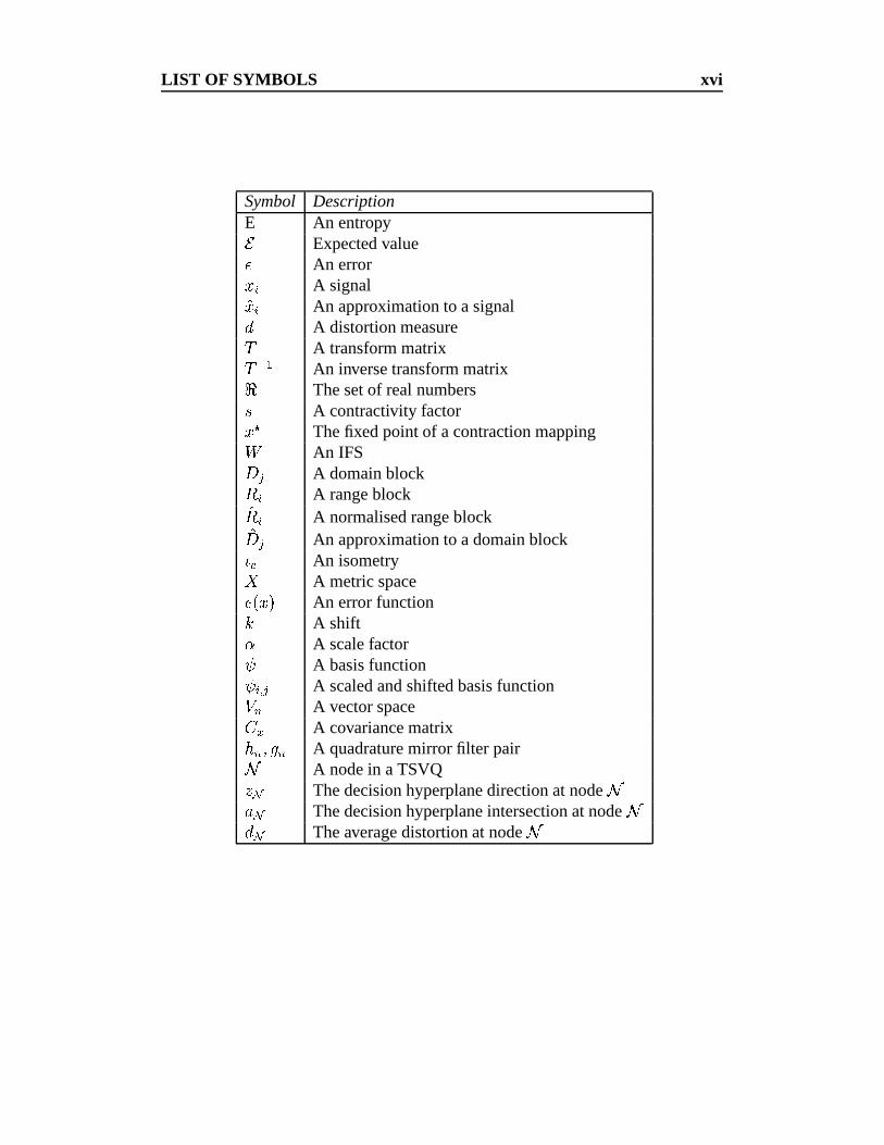
List of Symbols
This table contains a summary of the mathematical notation used in this thesis.
Note that only notation that carries meaning across a large part of the thesis is
listed. Also note that local definitions may supersede those listed here.
xv
LIST OF SYMBOLS xvi
Symbol DescriptionE An entropy�
Expected value� An error��� A signal���� An approximation to a signal�A distortion measure�A transform matrix���An inverse transform matrix�The set of real numbers� A contractivity factor�� The fixed point of a contraction mapping�An IFS
��� A domain block� � A range block�� � A normalised range block���� An approximation to a domain block��� An isometry�
A metric space������� An error function�A shift� A scale factor�A basis function� � � � A scaled and shifted basis function!#"A vector space�%$ A covariance matrix& "�')(*"A quadrature mirror filter pair+A node in a TSVQ,.- The decision hyperplane direction at node
+/0- The decision hyperplane intersection at node
+� - The average distortion at node
+
Chapter 1
Introduction and Scope of Thesis
1.1 Background
The recent explosion of global communication systems and interconnectivity has
resulted in massive growth of the number of connected computer users. These
users are connected by a common set of protocols, running over the physical me-
dia that have come to be known as the Internet. This explosion in the number of
users has, in turn, resulted in a dramatic increase in the amount of data passed over
the Internet. The World Wide Web (WWW) is an embodiment of the HTTP proto-
col and provides a rich, multimedia experience to anyone equipped with a piece of
browser software and an Internet connection. This multimedia experience consists
of text, images, audio and indeed video. As with any physical medium, the Inter-
net has bandwidth limitations. That is, the amount of data that can flow through
any point on the Internet in a given time period is limited. Now, a single im-
1
1.1 Background 2
age frame at broadcast television quality in monochrome occupies approximately
300kB of computer storage, roughly the same as a two hundred and fifty page text
document. Consequently, the shift towards multimedia communication and away
from plain text increases the volume of data to be transmitted by several orders of
magnitude. Couple this with the continual growth of the number of users and it is
simple to see that the limited bandwidth of the Internet is a significant constraint
on its usefulness. Methods of reducing the volume of data to be sent in all cases
are required.
The advent of high definition digital television (HDTV), cable TV, digital broad-
casting direct to homes and the possibility of “video-on-demand” over existing
telecommunication systems further increases the need for image and video com-
pression technologies. Given a standard Basic Rate Interface ISDN channel into
a home, the 128 kilobits per second bandwidth is soon used up by a simple video
stream alone. Consider an image that is approximately quarter TV-size (QCIF
format [Cla95]). This would consist of� ��� ��� � �
pixels, occupying � ��� � �
bits.
Given the��� � ��� � bandwidth, this would only allow three frames per second to
be transmitted, hardly enough for the viewer to perceive any motion at all and
certainly not even close to the quality produced by the current analogue television
system.
1.2 Digital Signal Representation 3
1.2 Digital Signal Representation
If digital systems cannot inherently match the quality of analogue ones, why
bother with them? In a digital transmission system, it is simple to differentiate
between signal and noise, unlike in the analogue system. The data that are sent
are exactly the data received. Thus, digital systems can operate over much larger
distances by the use of simple repeaters. Digital representations of signals also
allow computers and other digital processors to operate directly upon the data,
without conversion and the associated losses. Indeed, digital representations are
discrete and, as such, much simpler to operate upon than their analogue coun-
terparts. The advent of digital signal representations has made tractable many
problems that are intractable in the analogue domain. The applications made pos-
sible by the digital signal representation are too numerous to list. For example, in
image analysis parameters are extracted which somehow describe the content and
structure of an image in order to perform such tasks as object detection, recogni-
tion and classification. Image enhancement appears in many forms. For example,
reducing the amount of noise in an image so that it is more pleasing to the human
observer or false colouring images, such as satellite and medical images, to aid
human analysis.
In this thesis, it is always assumed that digital images are stored as a Cartesian
array of 8-bit integer values specifying the grey scale intensity at that point. The
array may be of arbitrary size, but will usually be� ��� � � � �
or����� � �����
elements
1.3 Foundations 4
Source Transmitter
Channel
Receiver Destination
Noise
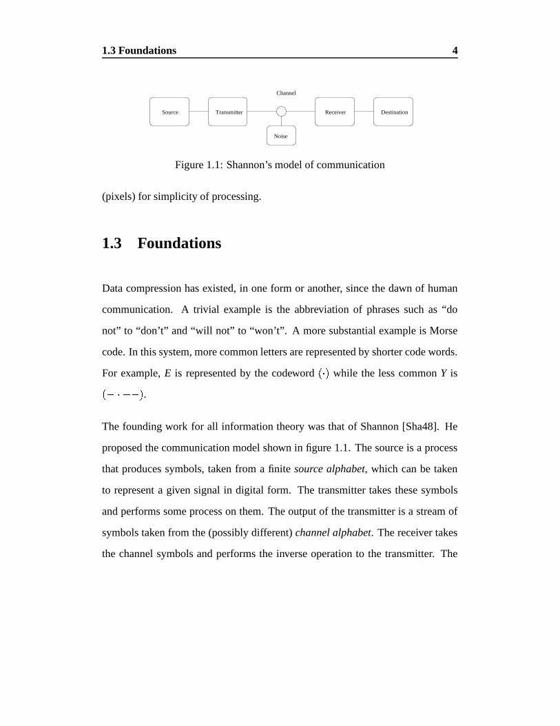
Figure 1.1: Shannon’s model of communication
(pixels) for simplicity of processing.
1.3 Foundations
Data compression has existed, in one form or another, since the dawn of human
communication. A trivial example is the abbreviation of phrases such as “do
not” to “don’t” and “will not” to “won’t”. A more substantial example is Morse
code. In this system, more common letters are represented by shorter code words.
For example, E is represented by the codeword ��� while the less common Y is
�� � ���
� .
The founding work for all information theory was that of Shannon [Sha48]. He
proposed the communication model shown in figure 1.1. The source is a process
that produces symbols, taken from a finite source alphabet, which can be taken
to represent a given signal in digital form. The transmitter takes these symbols
and performs some process on them. The output of the transmitter is a stream of
symbols taken from the (possibly different) channel alphabet. The receiver takes
the channel symbols and performs the inverse operation to the transmitter. The
1.3 Foundations 5
resultant signal is then passed to the destination.
It is prudent to further split the coding into source coding and channel coding.
Consider a channel with a capacity, � symbols per second, and a source with en-
tropy�
symbols per second. Assuming that��� � , Shannon, in his Fundamental
Theorem for a Discrete Channel with Noise [Sha48] stated that
It is possible to send information at the rate � through the channel
with as small a frequency of errors or equivocations as desired by
proper encoding.
This ensures that, given the output of an arbitrary source satisfying the entropy
constraint, it is possible to send this via the channel with arbitrary precision using
a suitable channel code. Thus, it is possible and also convenient practically, to sep-
arate source and channel coding: the former aims at producing the most efficient
representation of the source information, while the latter is aimed at minimising
the errors caused by the channel. The source coding problem can be seen as an
application of rate-distortion theory [Sha59] [Ber68] [Pin69]: given a fidelity cri-
terion, the task is to encode the source output to produce the minimum amount
of information. Conversely, given a maximum data rate, the task is to maximize
any fidelity measure (i.e. minimize any distortion measure). The minimizing of
the error and the amount of information to be transmitted is the goal of all data
compression algorithms.
This general communication model covers many processes and, in particular, im-
1.3 Foundations 6
age data compression. The purpose of the system is to reconstruct an approxima-
tion of the source data at the destination. The destination will usually be a human
observer and any distortion measures should reflect this fact. The channel may
be a physical channel, for example radio or optical fibre, or simply disk storage.
For the purposes of this thesis, the properties of the channel are moot since it is
concerned only with source coding, not channel coding. Indeed, in the two ex-
amples cited, the respective channel codings ensure “near lossless” delivery to the
destination.
The transmitter takes the source image and produces a stream of channel sym-
bols. If there are fewer channel symbols than source symbols, compression has
been achieved, assuming the cost of transmission is constant across all channel
symbols. If the operation performed by the transmitter is invertible, then the com-
pression is termed lossless, i.e. the reconstruction at the destination will be perfect.
If the operation performed is not invertible, then the compression is termed lossy
and a distortion measure is used to determine the quality of the reconstruction.
Shannon [Sha48] also defined the entropy of a signal. This is the minimum num-
ber of bits required to encode a given signal. If the signal values are independent,
then the entropy of the digitised signal is given by
� ��
����� �� ��� ��� �
�� � ��� � � (1.1)
where N is the number of symbols in the alphabet and � ��� � is the probability of the
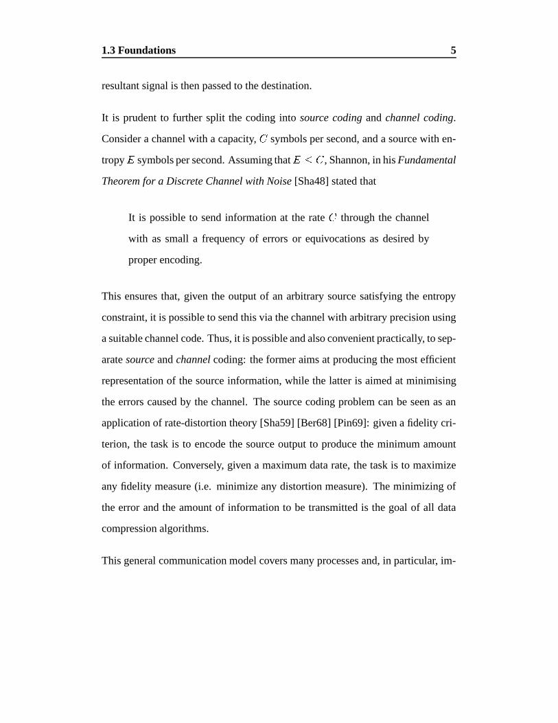
symbol � occuring. For the Lena image shown in figure 1.2, this gives an entropy
of� � � � bits per pixel. However, image pixel values are rarely independent and it
1.3 Foundations 7
Figure 1.2: Original Lena�������������
pixel image
is often prudent to take the previous value into account. This is measured via the
first order Shannon entropy, given by
� ��
��� � � � � �
����� � ����� � �� �
�� � ����� � � � (1.2)
where � ����� � � is the probability that symbol � will occur given that symbol�
has
just occurred. The first order entropy of the Lena image in figure 1.2 is� � � � bits
per pixel. It is common to utilise the correlation between samples in a signal.
By inspection, it is obvious that natural images have correlations that extend over
relatively large distances. These would not be fully accounted for by the first
order Shannon entropy, which only takes into account the immediately preceding
sample. One of the aims of this thesis is to derive methods of exploiting these
correlations, regardless of their distance or position.
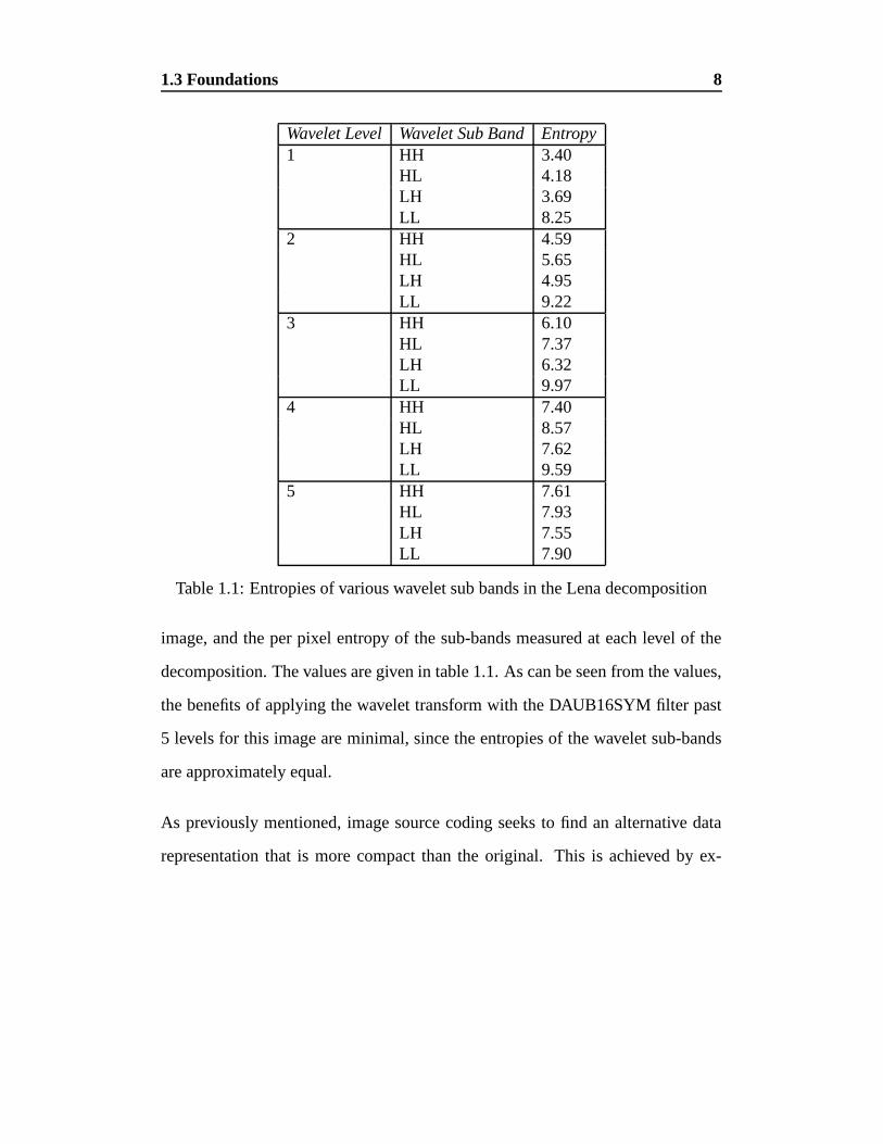
As an example, the wavelet transform (see chapter 2) was applied to the Lena
1.3 Foundations 8
Wavelet Level Wavelet Sub Band Entropy1 HH 3.40
HL 4.18LH 3.69LL 8.25
2 HH 4.59HL 5.65LH 4.95LL 9.22
3 HH 6.10HL 7.37LH 6.32LL 9.97
4 HH 7.40HL 8.57LH 7.62LL 9.59
5 HH 7.61HL 7.93LH 7.55LL 7.90
Table 1.1: Entropies of various wavelet sub bands in the Lena decomposition
image, and the per pixel entropy of the sub-bands measured at each level of the
decomposition. The values are given in table 1.1. As can be seen from the values,
the benefits of applying the wavelet transform with the DAUB16SYM filter past
5 levels for this image are minimal, since the entropies of the wavelet sub-bands
are approximately equal.
As previously mentioned, image source coding seeks to find an alternative data
representation that is more compact than the original. This is achieved by ex-
1.3 Foundations 9
ploiting the redundancies found in visual data, be it still images or video. In still
image compression, spatial redundancy, related to the spatial correlation, is abun-
dant. Indeed, there are large patches of near-constant tone in several places in the
Lena image. Video has an added dimension - time - and this introduces further re-
dundancies. Since adjacent frames of the video sequence must be similar for the
human visual system to perceive motion, there is obvious temporal redundancy
between frames. This is often exploited by only sending the frame differences,
which are obviously more compact than the full frame representation. A good
visual data compression system should exploit redundancy as efficiently as possi-
ble whilst also taking into account the characteristics of the human visual system
[Wat88], removing only the perceptually least relevant information.
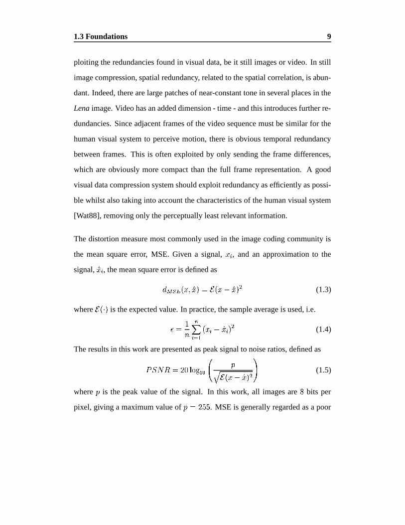
The distortion measure most commonly used in the image coding community is
the mean square error, MSE. Given a signal, ��� , and an approximation to the
signal,���� , the mean square error is defined as
� ����� ��� '��� � � � ����
�� � � (1.3)
where� ��� is the expected value. In practice, the sample average is used, i.e.
� � �
�"�
��� ������
���� � � (1.4)
The results in this work are presented as peak signal to noise ratios, defined as
�� � � � ��� �� � ��
�� � ����
���� ��
(1.5)
where�
is the peak value of the signal. In this work, all images are bits per
pixel, giving a maximum value of� � � � �
. MSE is generally regarded as a poor
1.4 The State of the Art 10
measure of visual quality, since the values are quickly skewed by a small number
of outlying values, and the measure does not take into account the properties of
the human visual system. However, it is very convenient analytically and can be
justified by observing that for small enough errors, � ��� "��"��� � �� , any distortion
measure will be approximately quadratic.
1.4 The State of the Art
Current visual data compression techniques broadly fall into the following cate-
gories :
Predictive Methods Predictive coders are simple to implement and computation-
ally efficient. They have been combined with a multitude of other tech-
niques in order to extend their usefulness [Jai89] [RC95] [LW96]. The main
problem with predictive coding is that it is effectively causal, whereas spa-
tial visual data is rarely so. That is, there is no obvious preferred direction
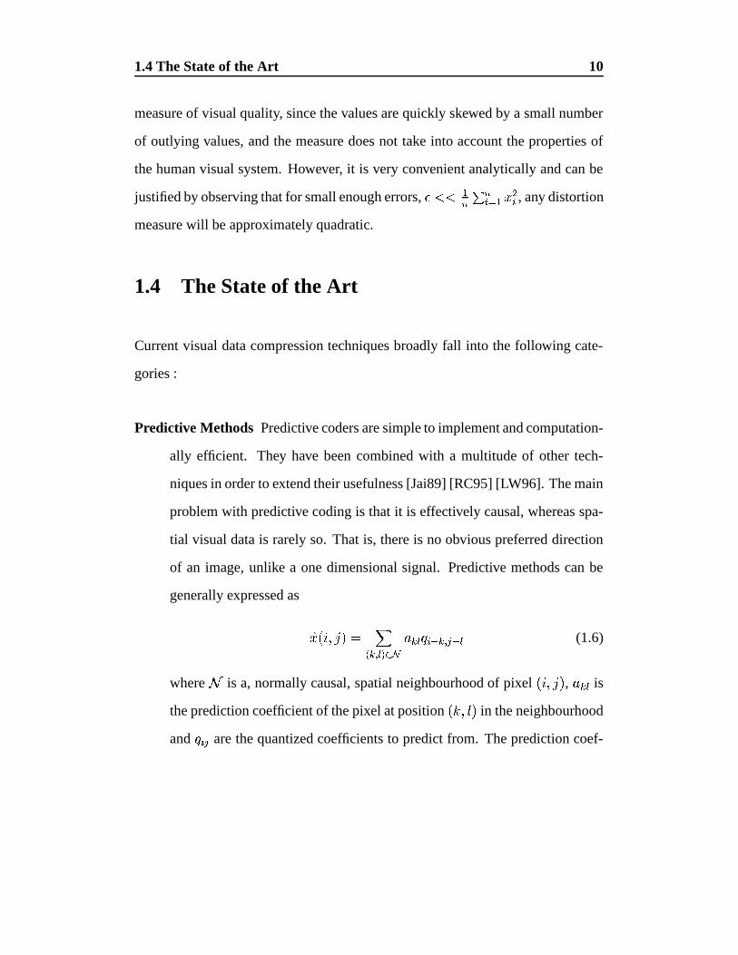
of an image, unlike a one dimensional signal. Predictive methods can be
generally expressed as
�� ��� ' � � � ���� � ��� -
/ � � � � � � � � � (1.6)
where+
is a, normally causal, spatial neighbourhood of pixel ��� ' � � , / � � is
the prediction coefficient of the pixel at position � � ' � � in the neighbourhood
and � � are the quantized coefficients to predict from. The prediction coef-
1.4 The State of the Art 11
ficients, / � � are either fixed or, in the case of adaptive prediction, estimated
locally.
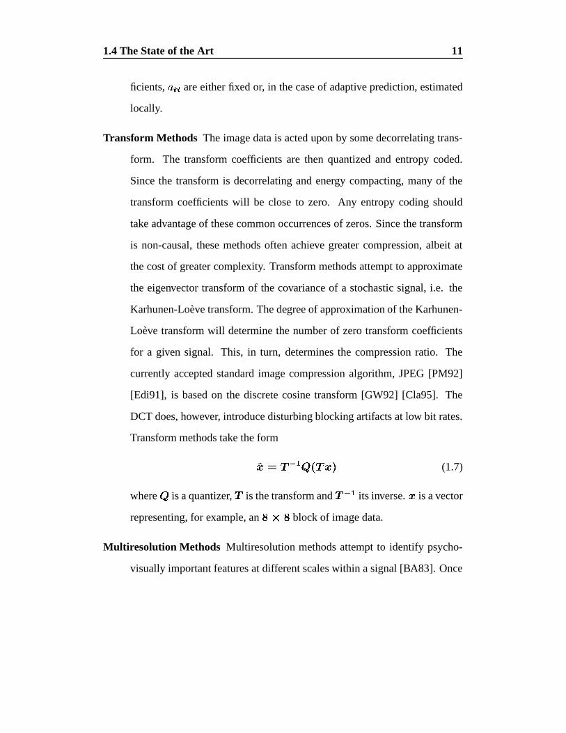
Transform Methods The image data is acted upon by some decorrelating trans-
form. The transform coefficients are then quantized and entropy coded.
Since the transform is decorrelating and energy compacting, many of the
transform coefficients will be close to zero. Any entropy coding should
take advantage of these common occurrences of zeros. Since the transform
is non-causal, these methods often achieve greater compression, albeit at
the cost of greater complexity. Transform methods attempt to approximate
the eigenvector transform of the covariance of a stochastic signal, i.e. the
Karhunen-Loeve transform. The degree of approximation of the Karhunen-
Loeve transform will determine the number of zero transform coefficients
for a given signal. This, in turn, determines the compression ratio. The
currently accepted standard image compression algorithm, JPEG [PM92]
[Edi91], is based on the discrete cosine transform [GW92] [Cla95]. The
DCT does, however, introduce disturbing blocking artifacts at low bit rates.
Transform methods take the form
���������� ������� (1.7)
where is a quantizer, � is the transform and � ��� its inverse. � is a vector
representing, for example, an � ��� block of image data.
Multiresolution Methods Multiresolution methods attempt to identify psycho-
visually important features at different scales within a signal [BA83]. Once
1.4 The State of the Art 12
the multiscale decomposition is complete, coding proceeds in a variety of
ways, pulling from both predictive and traditional transform methods. The
current benchmark for all image coding algorithms is Shapiro’s Embedded
Zerotree of Wavelet Coefficients coder (EZW) [Sha93]. It uses a wavelet
transform and encodes a given number of the coefficients using his novel
zerotree structure.
Fractal Methods Fractal methods have commonality with all the previous cod-
ing methods and also introduce new concepts. Fractal coding methods
are traditionally very computationally expensive and will be discussed at
length in chapter 2. They were popularised by Jacquin [Jac90] and Barns-
ley [Bar88] [BD85] [BH92].
Other Techniques Over the years, a variety of ad hoc approaches to compres-
sion, often motivated by properties of the visual system, have been put for-
ward (for example Graham’s contour coding method [Gra67]). More re-
cently, “model-based” coders using methods derived from computer graph-
ics have been explored [Pea95]. These techniques seldom have the robust-
ness and generality required to deal with the variety of images encountered
in all applications.
1.5 Thesis Outline 13
1.5 Thesis Outline
This thesis is concerned with novel methods of coding still images and video
sequences using the wavelet transform and its derivatives.
Chapter 2 provides an overview of the theory of iterated function systems, their
application to image compression, popularised by Jacquin [Jac90], and a general
review of fractal based image coding schemes. A novel analysis of the underlying
fractal basis follows and this leads to the description of the wavelet transform. The
chapter concludes with an overview of the state of the art of wavelet based image
coding schemes.
In chapter 3, a novel method of exploiting fractal coding methods in the wavelet
domain is described. A description of the machinery required for the Karhunen-
Loeve transform is interspersed with the actual coder description. Following from
this, the concept of orientation is introduced and related to the wavelet sub-band
decomposition. The effect of introducing the orientation estimate is investigated
in the simulation results.
Chapter 4 builds on the orientation concepts in chapter 3 by presenting a novel,
complex valued, oriented wavelet transform which retains many of the properties
of the traditional wavelet transform which are desirable in an image coding appli-
cation. A new tree structured vector quantizer algorithm is described, which uses
the Linde-Buzo-Gray [LBG80] method of codebook design internally for restruc-
1.6 Reproduction Limitations 14
turing. Chapter 4 concludes by combining these new concepts, and the concepts
of chapter 3, into a still image coding system. Results are presented for a variety
of parameter combinations and compared to current benchmark algorithms.
Chapter 5 presents an overview of video coding techniques, defines the three
dimensional, Cartesian separable wavelet transform and describes some of the
spatio-temporal properties of the transform. A novel linear quantizer based video
coding system is then described and results presented. The shortcomings of this
system are outlined and are then, to some degree, addressed by a video coder
based on the tree structured vector quantizer of chapter 4. The coder is exercised
on a variety of video sequences, at a variety of bit rates. Finally, comparisons are
drawn with current video coding techniques.
A review of the novel elements contained in the thesis is presented in the final
chapter along with conclusions and possible avenues of further research.
1.6 Reproduction Limitations
This thesis was printed on a Lexmark Optra 2450 laser printer. As a result, the
results contained herein are subject to printer artifacts which may be mistaken for
coding artifacts.
Chapter 2
Iterated Function Systems and theWavelet Transform
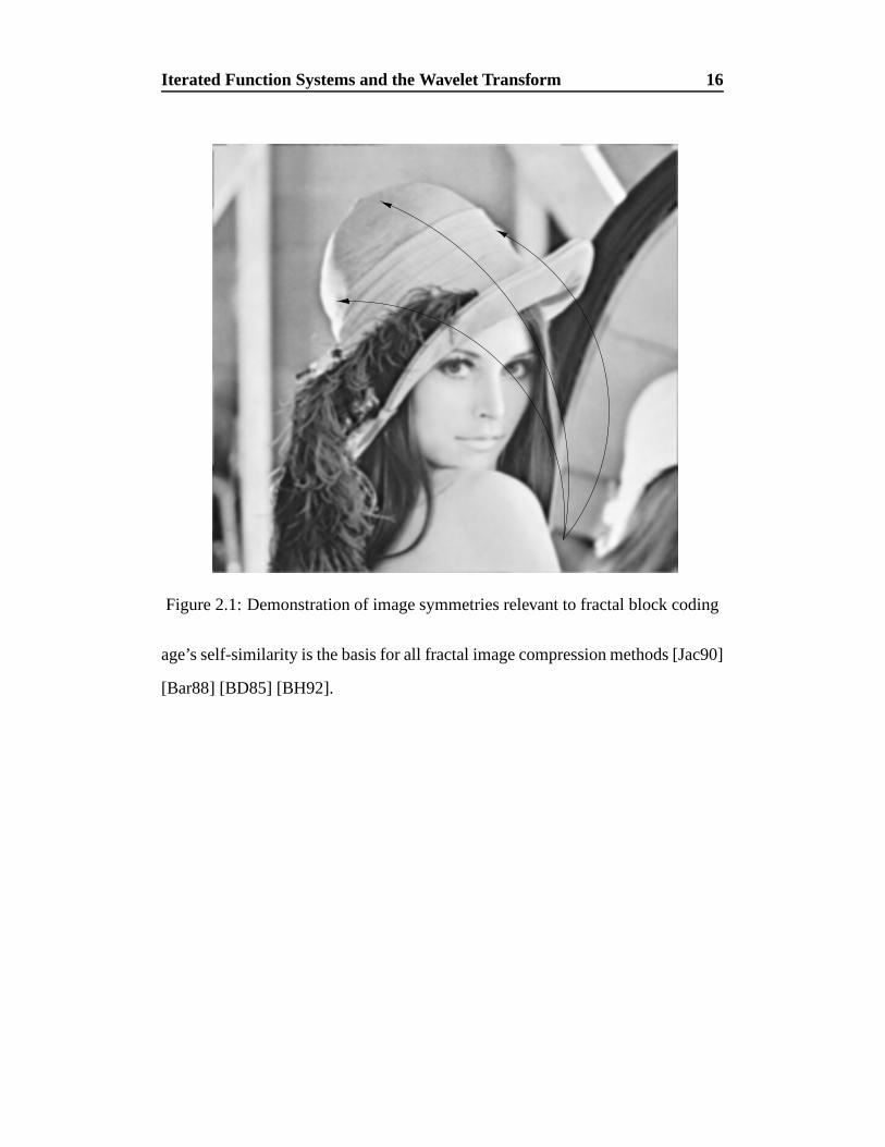
Image data should naturally contain patches of similar detail at the same and dif-
ferent scales. Consider a forest scene. As the scale at which the scene is viewed
changes, certain similarities become apparent. For instance, leaves on the left and
right side of a tree would look similar, up to a rotation of � , and from a large
distance, a whole tree may appear similar to a leaf viewed close up. The relevance
of this form of symmetry in image representation has been discussed at length
by Barnsley [Bar88] [BD85] [BH92]. Fractal image compression relies on this
premise. To demonstrate the relevance of image symmetry to this method, refer
to figure 2.1. The block at the bottom of the image (the source block) may be
used as a template for the other blocks (target blocks) shown in the figure. Ap-
proximations to the target blocks are created from the source block by appropriate
rotations and flips around the mid-point axes. This simple expression of an im-
15
Iterated Function Systems and the Wavelet Transform 16
Figure 2.1: Demonstration of image symmetries relevant to fractal block coding
age’s self-similarity is the basis for all fractal image compression methods [Jac90]
[Bar88] [BD85] [BH92].
2.1 Fractal Block Coding and Iterated Function Systems 17
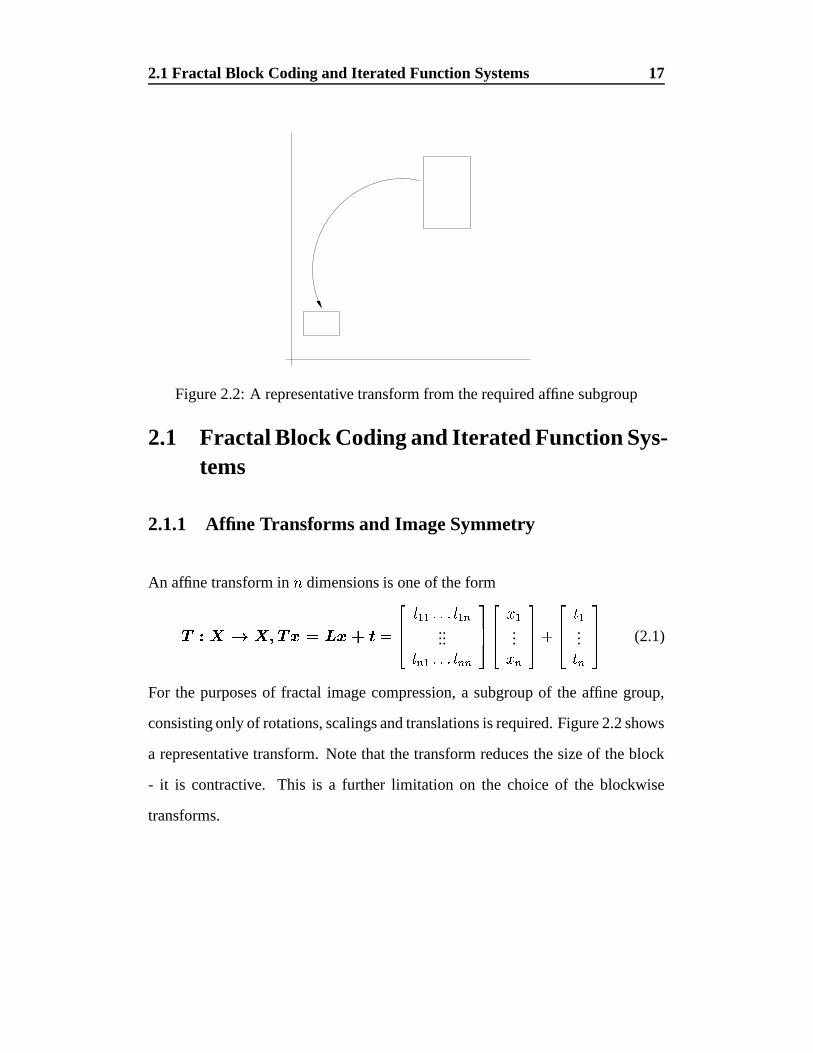
Figure 2.2: A representative transform from the required affine subgroup
2.1 Fractal Block Coding and Iterated Function Sys-tems
2.1.1 Affine Transforms and Image Symmetry
An affine transform in � dimensions is one of the form
� ��� � ��� � ����� ��� �� �� � � � � "
......� " � � � � " "
������ �
� ...� "
�������
� �� ...� "����� (2.1)
For the purposes of fractal image compression, a subgroup of the affine group,
consisting only of rotations, scalings and translations is required. Figure 2.2 shows
a representative transform. Note that the transform reduces the size of the block
- it is contractive. This is a further limitation on the choice of the blockwise
transforms.
2.1 Fractal Block Coding and Iterated Function Systems 18
Fractal block coding is based on the ground-breaking work of Barnsley [Bar88]
[BD85] [BH92] and was developed into a practical algorithm by Jacquin [Jac90].
The concept underlying this technique is that for each image, there exists a block-
wise transform upon the image that will leave it unchanged. The roots of fractal
block coding lie in the mathematics of metric spaces and, in particular, the Con-
traction Mapping Theorem.
2.1.2 The Contraction Mapping Theorem
Definition 2.1.1 (Contraction Mapping) Let � � ' � � be a complete metric space.
That is let�
be a vector space over some field�
and�
be a metric upon�
. Then,
a transformation�
,���*��� �
is said to be a contraction mapping if and only if
� ��� � ' � � � � � � � � � � � ����� ')� ��#�)� � ��
� � � ' �#�� � ' ��� � � (2.2)
Here, � is known as the contractivity factor of the transformation�
.
Theorem 2.1.1 (Contraction Mapping Theorem) For a contraction mapping�
on a complete metric space�
, there exists a unique fixed point � � �such that
� � � ��� � . The unique fixed point is then
� � ���������� � � ��� � � ' � � � �
For proof and the Collage theorem, see Appendix A.
2.1 Fractal Block Coding and Iterated Function Systems 19
Theorem 2.1.1 states that if a contraction mapping is iterated, there exists a point
where further application of the mapping has no effect. The point at which this
occurs is called the fixed point of the contraction mapping and, remarkably, is in-
dependent of the initial conditions of � � . Define an Iterated Function System (IFS)
[BD85] [Bar88] [BH92] as a set of contraction mappings� � ��� " � � � � ' � � � ' ��� ' � " �
� � �with contractivity factors � "
. Then, the IFS is itself a contraction map-
ping on�
and has contractivity factor � ��� / � � � " � . Note that, implicit to the
IFS definition, is the domain and range of each map. Each map has distinct do-
main on�
, usually a compact, non-empty subset of�
. Now, since the IFS is a
contraction mapping on�
, it too has a unique fixed point � � �. Since �# is
unique, it is completely specified by the IFS,�
. The image processing problem,
termed the inverse problem by Barnsley [BH92] is then “Given an image � , can
an IFS,�
, be found such that the fixed point of�
is � ?” At the present time,
there is no general method for finding such an IFS, given � . However, using the
IFS fixed point equation
� � � ��� � � � ��� ��� � �� � " ��� � '
(2.3)
where � � � represents the ‘pasting together’ of transformed patches, and the Col-
lage Theorem (section A.2)
� � � ' � � � �
��
� � � � ' � � � � � (2.4)
an approximation method can be constructed. Equation 2.3 states that to find the
IFS�
, a set of contractive transforms should be applied to � and the resultant
patches pasted together to reconstruct � . The uniqueness of � is important since
2.1 Fractal Block Coding and Iterated Function Systems 20
w1 w2
w3 w4
W W W
(b)
(a)
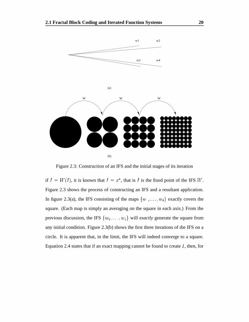
Figure 2.3: Construction of an IFS and the initial stages of its iteration
if � � � � � � , it is known that � � �# , that is � is the fixed point of the IFS�
.
Figure 2.3 shows the process of constructing an IFS and a resultant application.
In figure 2.3(a), the IFS consisting of the maps� � ' � � � ' � � � exactly covers the
square. (Each map is simply an averaging on the square in each axis.) From the
previous discussion, the IFS��� ' � � � ' � � � will exactly generate the square from
any initial condition. Figure 2.3(b) shows the first three iterations of the IFS on a
circle. It is apparent that, in the limit, the IFS will indeed converge to a square.
Equation 2.4 states that if an exact mapping cannot be found to create � , then, for
2.1 Fractal Block Coding and Iterated Function Systems 21
largely contractive maps (i.e. those with � ��� �), the more similar the union of
the IFS-generated patches is to � , the closer �� will be to � . The obvious question
is then “Why not make�
slightly contractive on I?” Then� � � ' � � � � � will be
small. However, the factor � � will be large and there is then no guarantee that
� � � ' �� � will be small.
Note that the sequence � � ' � ��� � � ' � � ��� � � ' � � � is a Cauchy sequence in�
( see
Appendix A for details). Now,�
is complete and therefore the limit of the Cauchy
sequence, the fixed point of the IFS, is in�
. However, it is not possible to state
that, for all � � �, there exists a Cauchy sequence of mappings (and therefore an
IFS) in�
with limit point � . Thus, it is not possible to say with absolute certainty
that fractal image compression methods can exactly reconstruct any image. More-
over, there may be an open set around a point in�
which contains no limit points
of any Cauchy sequence. It is therefore impossible to say how closely a fractal
image compression system can approximate an arbitrary image. This represents a
fundamental weakness in a general purpose image coding method.
2.1.3 Fractal Block Coding
Fractal block coding, as described by Jacquin [Jac90], is a notoriously slow and
computationally intensive process. Given an arbitrary image�
, it is partitioned
into non-overlapping blocks,� � � � of size
� � �. These blocks will be known as
domain blocks, following the notation
of Barnsley [BH92]. The image is then�Barnsley’s notation is slightly confusing since it refers to the inverse transform.
2.1 Fractal Block Coding and Iterated Function Systems 22
Ordinal Isometry1 Identity2 Flip along mid-X axis3 Flip along mid-Y axis4 Flip along major diagonal
Table 2.1: Base isometry set used in conventional fractal block coders
spatially averaged by 2 in both the horizontal and vertical directions, extracting
all, possibly overlapping, blocks of size� � �
producing the pool of range blocks,� � � � . The goal of a fractal block coder is then to find the optimal parameter set� / ' � ' � ' � � for each block � � in the approximation
���� � /
���� � � � � � � � � � � � � � (2.5)
such that the error� � � � ' �
� � � is minimised. It is usual for�
to be the metric
derived from the���
norm, � � � � �� ��� � , the squared error measure. The set
� � � �is the set of isometries generated by the dihedral group of the square. Table 2.1
shows the base isometries which are combined to form the eight isometries of
the square. The fractal block code for the image then consists of the parameter set� / ' � ' � ' � � for each domain block � � in the domain pool
� � � � . The parameter sets
are entropy coded to provide compression. Note that the parameter set� / ' � ' � ' � �
is restricted since the final transform� ��� � � � must be a contraction mapping
under the metric�. Jacquin [Jac90] notes that the isometries all have unity � � -
contractivity and the contrast scale by / has � � -contractivity of / � . Hence, to
ensure that the transform for each block is a contraction mapping, the value of /
must be restricted such that� � / � �
. This, in turn, limits the contrast scalings
to dynamic range reductions. Then, if all the block transforms are contraction
2.1 Fractal Block Coding and Iterated Function Systems 23
mappings, the union of the block transforms is itself a contraction mapping.
Reconstruction of the approximation to the image�
from the fractal block code
follows from the Contraction Mapping Theorem and the Collage Theorem. Note
that� � � � � � is, by the Collage Theorem, a contraction mapping. There-
fore, by the Contraction Mapping Theorem,�
has a unique fixed point, � �
����� " ��� � " ��� � � . Since the blockwise component contraction mappings were cho-
sen to minimize the individual errors, their union minimizes the overall error.
Hence, the unique fixed point will, in some sense, be close to�
. Reconstruction,
therefore, is simply a matter of iterating the maps on any initial image, spatially
averaging by two between the iterations. The choice of initial image is irrele-
vant since, by the Contraction Mapping Theorem, the fixed point � �
is unique.
Therefore, � � � ' ����� $ ��� � " ����� � � �
. The iterative reconstruction process is
continued until some specified error condition has been met or until the difference
between successive iterations is below some threshold.
2.1.4 Properties and pitfalls of the fractal method
Fractal image compression has suffered, from the outset, claims of extreme com-
pression ratios [BH92]. These extreme claims have come about because of the
resolution independence of the fractal block coding method. That is, it is possible
to generate the fractal block code for an image of� ��� � � ���
pixels and reconstruct
it at��� � � � ��� � �
pixels (since the maps are resolution independent), resulting in
an apparent increase of 16 times in the compression ratio. The resolution indepen-
2.2 Advances in Fractal Block Coding Algorithms 24
dence of the method also allows so called infinite zooming. Again, a zoomed area
is reconstructed at a higher resolution. The iterative method will add false detail
to the zoomed image, making it more pleasing to the casual observer. However, it
is important to note that any detail added is, of course, interpolated false detail : it
increases the overall error.
Moreover, fractal image compression is a highly asymmetric process; that is, cod-
ing takes much longer than decoding. This is due to the extensive nature of the
domain block search. This can be a disadvantage in some applications.
2.2 Advances in Fractal Block Coding Algorithms
Much research has revolved around speeding up the coding in some way. Jacquin
[Jac90] suggested classifying the range blocks into three distinct classes: shade
blocks, midrange blocks and edge blocks. The coder then only checks range
blocks in the same class as the current domain block when searching for the op-
timal transform. Details of the classification algorithm used by Jacquin can be
found in [RA86].
Jacobs, Fisher and Boss [JFB92] classify blocks into 72 different classes and also
apply a quadtree partitioning scheme. The quadtree scheme works by using larger
blocks ( � � � in their paper) and splitting the block into four smaller blocks
should an error condition not be satisfied. This quadtree decomposition is repeated
until the error condition is satisfied or a minimum block size is reached. This
2.2 Advances in Fractal Block Coding Algorithms 25
has obvious advantages if parts of the image contain large regions of relatively
constant greyscale.
The same authors [JFB91] proved that not all the� � in the IFS
� � � � � ' � � � ' � " �
need to be contractive. They define a map� ��� � �
as eventually contractive
if, for some � ����� ,� "
is contractive. They then prove that the fractal de-
coder will converge if� � � � � � is only eventually contractive. Here, the iterated
transform���
is the composition of transform unions of the form
� ��� � �� �� � � � � � ��� �
Since the contractivities of each union� ��� multiply to give the overall contrac-
tivity of the iterated transform, the composition may be contractive if it contains
sufficiently contractive� ��� . Intuitively, it is simple to see that if the union consists
of slightly expansive transforms and highly contractive ones, then the union will
eventually be contractive. The provision for eventually contractive maps allows
the coder to achieve better results. Since there is now no longer a bound on the
contractivity of the component transform , the dynamic range of range blocks may
now be increased to be similar to that of the domain block.
Most speed-ups have reduced the size of the pool that the coder must search for
each domain block in some way. Reducing the size of the search pool, however,
can have an adverse effect on reconstructed image quality since the range block
pool is not as rich. Saupe [Sau95] uses the theory of multi-dimensional keys
to perform an approximate nearest-neighbour search. Since this search can be
completed in � ��� ( � � time, the range pool need not be depleted to achieve a
2.2 Advances in Fractal Block Coding Algorithms 26
speed up. Saupe’s basic idea is that of a � ��
� �� dimensional projection on
� �
where��� �
. He defines a subspace,��� � �
as� � � ��� ���
�� � � � � � where
� � � � � ' � � � ' � � � � �. Defining �
�
'�� to be the inner product operator and a
normalised projection operator � � ��� �and a function � � � � � � � '�� ���
by
� � ��� � ��
� � ' � �� � � � � ' � � �
and
� � � ' , � � � ��� � � � � ����� ' � � , � � ' � �� � ����� ' � � , � �)�
gives an expression for the squared error
� � � ' , � � � , ' � � , � � ( � � ��� ' , � �
where( � � � � � � � � � � ��� � � . This theorem states that the squared error,
� � � ' , �
is proportional to( � � � which is a simple function of the Euclidean distance be-
tween � � ��� and � � , � ( or � � � ��� and � � , � since � ����� is unique up to sign). Note
also that(
is monotonically increasing on the interval � ' � ���
. Saupe then states
that the minimisation of the squared errors� � � � ' , � � � � ' � � � ' � is equivalent
to the minimisation of the � ��� � ' , � . Thus, the squared error minimisation may be
replaced by the nearest neighbour search for � � , � � � �in the set of
� � vectors� � � ��� � � � �
. Since� �
is a Euclidean space, any of the nearest neighbour search
algorithms that run in expected logarithmic time, for example kd-trees [FJF77],
can be applied. Saupe does, however, note that an � block results in 64 dimen-
sions for the multi-dimensional keys. He therefore suggests downsampling the
blocks to, say,� � �
which reduces storage requirements to just 16 dimensions.
2.2 Advances in Fractal Block Coding Algorithms 27
Other speed up methods have revolved around performing little or no searching
for the range blocks. Monro et al [MWN93] [MDW90] [Mon93] [MD92] , have
developed and patented a technique known as the Bath Fractal Transform � (BFT).
The BFT works by limiting the search of the range blocks and also using higher
order functions on the blocks. Mathematically, if� � � � � � � ' � � � ' � � � ' � �
is an IFS with attractor A, they define a fractal function�
on � as� � � � ��� ' ��� � �
� � � � ' � ' � ��� ' ��� � , where the maps � � have parameters � ��� �� ' � � � ' � � � ' � ' � �� ' � � ��� . Then, � is the order of the IFS and � is the number of free parameters
of the BFT. The function�
is found by minimising� � (�' �( � for some suitable metric
�over block
�where
�( ����� � � � � � ��� � ��� ' ( � � ��� � ��� � � '
(is the original image greyscale values and
�(is the approximation. Solving
� � � (�' �( �� � � � ��
� � � ' �
gives the BFT. They define various searching options for the BFT, defined before
downsampling has occurred; that is, they assume that domain blocks are� � �
while range blocks are� � � � �
. A level zero search chooses the range block in
the same position as the domain block. A level one search would include the
four range blocks that intersect the domain block. A level two search would also
include all range blocks that intersect those in level one and so on. The complexity
options used, however, make the BFT unique. As it stands, such a limited search
would severely degrade reconstructed image quality. Allowing higher order terms�They are at Bath University, England.
2.2 Advances in Fractal Block Coding Algorithms 28
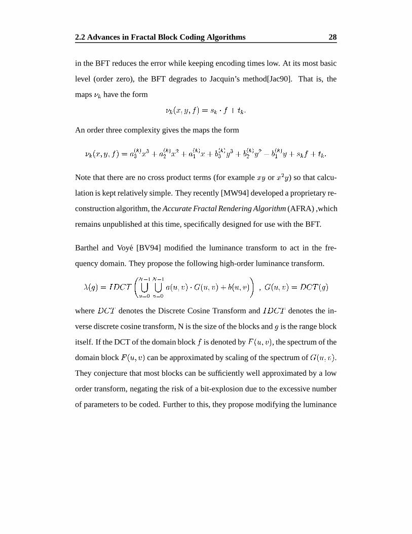
in the BFT reduces the error while keeping encoding times low. At its most basic
level (order zero), the BFT degrades to Jacquin’s method[Jac90]. That is, the
maps � � have the form
� � ��� ' � ' � � � � � � � � � � �An order three complexity gives the maps the form
� � ��� ' � ' � � � / � � �� � � � / ��� ��
� � � / ��� � � � � ��� �� � � � � ��� �� � � � � ��� � � � � � � � � � �Note that there are no cross product terms (for example � � or � � � ) so that calcu-
lation is kept relatively simple. They recently [MW94] developed a proprietary re-
construction algorithm, the Accurate Fractal Rendering Algorithm (AFRA) ,which
remains unpublished at this time, specifically designed for use with the BFT.
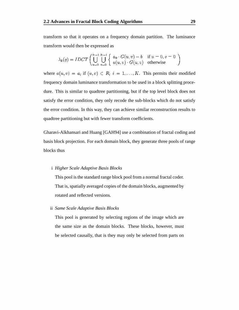
Barthel and Voye [BV94] modified the luminance transform to act in the fre-
quency domain. They propose the following high-order luminance transform.
� � ( � � � � � ��� � ���� � �� ���� � � / ��� ' �
��� ��� ' � � � � � ' ��� ' � � � ' � � � � � � ( �
where � � �denotes the Discrete Cosine Transform and � � � �
denotes the in-
verse discrete cosine transform, N is the size of the blocks and(
is the range block
itself. If the DCT of the domain block�
is denoted by� ��� ' � , the spectrum of the
domain block� ��� ' � can be approximated by scaling of the spectrum of � ��� ' � .
They conjecture that most blocks can be sufficiently well approximated by a low
order transform, negating the risk of a bit-explosion due to the excessive number
of parameters to be coded. Further to this, they propose modifying the luminance
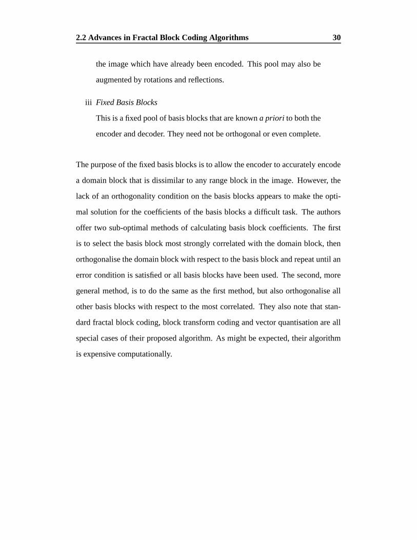
2.2 Advances in Fractal Block Coding Algorithms 29
transform so that it operates on a frequency domain partition. The luminance
transform would then be expressed as
� � � ( � � � � � � � � ���� � �� ���� � �
� / � � � ��� ' � � � if � � � ' � �/ � � ' �
��� � � ' � otherwise�
where / ��� ' � � / � if � � ' � � � � � � � ' � � � '�� . This permits their modified
frequency domain luminance transformation to be used in a block splitting proce-
dure. This is similar to quadtree partitioning, but if the top level block does not
satisfy the error condition, they only recode the sub-blocks which do not satisfy
the error condition. In this way, they can achieve similar reconstruction results to
quadtree partitioning but with fewer transform coefficients.
Gharavi-Alkhansari and Huang [GAH94] use a combination of fractal coding and
basis block projection. For each domain block, they generate three pools of range
blocks thus
i Higher Scale Adaptive Basis Blocks
This pool is the standard range block pool from a normal fractal coder.
That is, spatially averaged copies of the domain blocks, augmented by
rotated and reflected versions.
ii Same Scale Adaptive Basis Blocks
This pool is generated by selecting regions of the image which are
the same size as the domain blocks. These blocks, however, must
be selected causally, that is they may only be selected from parts on
2.2 Advances in Fractal Block Coding Algorithms 30
the image which have already been encoded. This pool may also be
augmented by rotations and reflections.
iii Fixed Basis Blocks
This is a fixed pool of basis blocks that are known a priori to both the
encoder and decoder. They need not be orthogonal or even complete.
The purpose of the fixed basis blocks is to allow the encoder to accurately encode
a domain block that is dissimilar to any range block in the image. However, the
lack of an orthogonality condition on the basis blocks appears to make the opti-
mal solution for the coefficients of the basis blocks a difficult task. The authors
offer two sub-optimal methods of calculating basis block coefficients. The first
is to select the basis block most strongly correlated with the domain block, then
orthogonalise the domain block with respect to the basis block and repeat until an
error condition is satisfied or all basis blocks have been used. The second, more
general method, is to do the same as the first method, but also orthogonalise all
other basis blocks with respect to the most correlated. They also note that stan-
dard fractal block coding, block transform coding and vector quantisation are all
special cases of their proposed algorithm. As might be expected, their algorithm
is expensive computationally.
2.3 Connection with Conventional Coding Methods 31
2.3 Connection with Conventional Coding Methods
Fractal image compression, in all its forms, can be seen as a mapping from im-
age to image. Conventional predictive image coding [Jai89] is also defined as a
mapping from image to image of the form
� � � � � � (2.6)
where A is a linear predictor matrix and�
is the prediction error. In conventional
linear prediction, � is a causal predictor. That is, � relies only on data previously
coded to form its predictions. The prediction function is often modified on a per-
pixel basis in order to obtain the best prediction at any point. Since it is causal,
the same prediction operation can be performed at both the encoder and decoder
and so the predictions generate no extra information. Most computation in con-
ventional predictive coding is concentrated on encoding�, the prediction error,
as compactly as possible. Prediction in this framework is usually on a per-pixel
basis. Now, fractal image compression works in much the same way, although
the prediction is applied to blocks and the predictor is modified on a per-block
basis and consequently some data must be sent to encode the predictor parame-
ters. The parameters in fractal coding determine the position and scale factor of
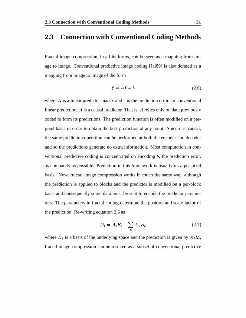
the prediction. Re-writing equation 2.6 as
�� � � � � � � � �
�� � � � (2.7)
where � is a basis of the underlying space and the prediction is given by � � � � ,fractal image compression can be restated as a subset of conventional predictive
2.3 Connection with Conventional Coding Methods 32
methods.
Image data compression methods can be analysed from the viewpoint of the basis
that they use to represent the data. The conventional linear predictive method,
detailed above, trivially has a complete basis generated by the impulse values
from the error term�
in equation 2.6 or the error correction terms� � � � in equa-
tion 2.7. What is the basis presented by conventional blockwise fractal compres-
sion methods? Fractal compression proceeds via averaging, dyadic downsampling
and shifting to form the prediction pool and addition of constant blocks to handle
errors. The characteristics of the basis depend solely on the block size. If the
block size is one pixel then, trivially, the system can encode any signal as a linear
combination of impulses. In this case, the basis is (over) complete. If the block
is the same size as the image , then, again trivially, the basis is constant. Fractal
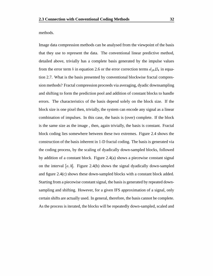
block coding lies somewhere between these two extremes. Figure 2.4 shows the
construction of the basis inherent in 1-D fractal coding. The basis is generated via
the coding process, by the scaling of dyadically down-sampled blocks, followed
by addition of a constant block. Figure 2.4(a) shows a piecewise constant signal
on the interval / ' � �
. Figure 2.4(b) shows the signal dyadically down-sampled
and figure 2.4(c) shows these down-sampled blocks with a constant block added.
Starting from a piecewise constant signal, the basis is generated by repeated down-
sampling and shifting. However, for a given IFS approximation of a signal, only
certain shifts are actually used. In general, therefore, the basis cannot be complete.
As the process is iterated, the blocks will be repeatedly down-sampled, scaled and

2.3 Connection with Conventional Coding Methods 33
a b(a)
(b)
(c)
Figure 2.4: The basis created by the fractal block coding scheme
2.3 Connection with Conventional Coding Methods 34
a constant block added. Now, since the scale factor used must be strictly less than
unity, the constant value added cannot be identically zero. If it were, the energy
in the blocks would decay to zero as the iteration progressed. This, in turn, would
imply that all the allowed iterated function systems would, in the limit, iterate to
zero. Hence, the constant block value cannot be identically zero and, therefore,
arbitrary impulses cannot be represented. It follows that, given the basis generated
by the fractal scheme, perfect reconstruction of an arbitrary signal is impossible,
since the basis is not complete (and neither is its closure). This is obviously a ma-
jor weakness of the conventional fractal block coding method : it cannot guarantee
perfect reconstruction of an arbitrary image. As a concrete example, consider the
signal� � '�
� ' � '�
� ' � � � ' � � � . Any even length block in this sequence will av-
erage to a piecewise constant block of value zero. The addition of any constant
block will obviously be unable to reproduce the original sequence, and the clos-
est approximation to the block� � '�
� ' � '�
� � is given by� � ' � ' � ' � � . To remedy
this defect, it would obviously be possible to augment the constant by a vector set
which is complete on the block, such as the discrete cosine transform. Is there a
natural basis set for this purpose?
Consider a fractal block transform of the form
� � ��� � � � � �� �
� � � ������� � (2.8)
Assuming that� � � � , this can be expressed as
� � � � � � � � � � ��� � � � � � � � � � � � � �� �
� � � ������� (2.9)
2.3 Connection with Conventional Coding Methods 35
where� � � � is some suitable orthogonal basis of � � . Now, define
� � � � to be
� � � � � � � �� � � ��� � � (2.10)
which, if� � � � � � � , implies
� � � � � �� �
� � � � ����� � ������ �
��� �� � � $
� ��� �� �� � �
��� � � � � $
� ��� �� � �� � �
��� �� � � $
� ��� �� � � � � � �
� � � � � � � � � � � � � ��� �
(2.11)
Substituting (2.11) into (2.9) gives
� � � � � � � � � � ��� � � � � � � � � � � � � � � � � � � � ��� � �������� � � � � � �� � � � � � � � � � � � � ��� � ������� (2.12)
Therefore,� � � � � � � � � �� � � � � � � � � � � � � (2.13)
This states that, if the basis generated by equation 2.10 is used, the coefficients
of� � should be predicted from the coefficients of
� � �� by the fractal block coding
algorithm. Furthermore, if the basis� � � � � � is an orthonormal one, then the scale
spaces� � are all orthonormal. Thus, the error coefficients �0� � � are orthogonal for
each � . This treatment does, however, require that the shift,� �
is a multiple of� � � .
This restriction does not practically challenge the validity of the argument due to
the shift invariance and stationarity of the data. The next section makes rigorous
the construction and properties of the basis� � � � .
2.4 The Wavelet Transform 36
2.4 The Wavelet Transform
The Fourier Transform method is a well known tool for signal analysis. The
Fourier Transform expresses any square integrable�
� periodic function on � � � � ' ��� �
as the projection of it onto the orthonormal basis
� " � ��� � ��� " $ ' � � � � � ' � � ' � ' � ' � � � �
However, if � ����� � � � $ then �" � � ��� ��� . Hence, the orthonormal basis
�� " � is
actually the set of integer dilates of the single function � . Note that
� ����� � ��� $ ��� ���� � ��� ��� � �
A remarkable fact about the Fourier Transform is that this is the only function
required to generate all� � periodic square integrable functions. One problem
with the Fourier transform is that of locality. Fourier basis functions are localised
only in frequency, not in time. This implies that any errors in the Fourier transform
coefficients will produce errors that are localised in frequency, but which spread
throughout the whole time domain. This property is one which has adverse effects
on image coding schemes. A transform which has basis functions localised in both
frequency and time would be preferable [Wil87].
2.4 The Wavelet Transform 37
2.4.1 The Continuous Wavelet Transform
The space � � � � � is practically more useful than � � � � ' ��� � [Mal89]. Functions
in � � � � � satisfy the following condition
� �� � � � ����� � � � � ��� �
Since every function in � � � � � must decay to zero at� � , the Fourier basis func-
tions �", which are sinusoids, are not in � � � � � . A synonym for sinusoids is waves
and if it is required that waves generate � � � � � , they must decay very quickly to
zero (for all practical purposes). Hence, small waves or wavelets are needed to
generate � � � � � . As in the Fourier Transform case, the wavelets should ideally
be generated by one function. However, if the wavelets must decay to zero, the
function dilates must be translated along�
by integral shifts in order to cover�
.
Given a mother wavelet� � � � � � � of unit energy, then all the translated dilates
� � � � ����� � � ��� � � � � � ��
� � ' � ' � � �
also have unit energy.
Definition 2.4.1 (Wavelet) A function� � � � � � � is called a wavelet if the family
� � � � � � defined by
� � � � ����� � � ��� � � � � � ��
� � ' � ' � � �
is an orthonormal basis of � � � � � . That is
� � � � � ' � � � � ��� � � � � � � � ' � ' � ' � ' � � �
2.4 The Wavelet Transform 38
where
� � � � �� �
if� � �
�otherwise
Then, every� � � � � � � can be written as
� ����� ���
� � � � � �� � � � � � � � � ��� � (2.14)
The series representation of�
in 2.14 is called the wavelet series of�
and is anal-
ogous to the Fourier series of a function. Similarly, the integral wavelet transform
[Chu92] may be defined, analogous to the continuous Fourier Transform as
� � �� � � � ' / � � � / � �� � � �
�
� �� � ��� � � �
�
�/ � � � ' � � � � � � � �
Wavelets are localised both in frequency (scale) by dilations and in time by trans-
lations. Errors in the coefficients will produce errors which are localised in both
frequency and time, unlike the Fourier transform as detailed in section 2.4.
2.4.2 The Discrete Wavelet Transform
The continuous wavelet transform is a useful theoretical tool, but image process-
ing deals with sampled images, i.e discrete values. A simple and fast method of
calculating the wavelet coefficients of a signal is required. Daubechies [Dau88]
defines the 1-D discrete wavelet transform in terms of a pair of quadrature mirror
filters (QMF pairs) [Dau92] [AH92]. If� ( " � is a sequence that is generated by
sampling the mother wavelet�
, then(
will be a high pass filter. The mirror filter
2.4 The Wavelet Transform 39
of this is� & " � , given by the relation
( � � ��
� � � & � � . The discrete wavelet
transform is then defined in terms of successive filtering and dyadic downsam-
pling. � �" � � � & � � � �� � � ��
� �� �" � � � ( � � � �� � � �
�
� �where � � ��� � � � ��� � is the original signal and the wavelet transform coefficients
consist of� � �" � . For reconstruction, it is usual to zero pad the data with
� ��
�
zeros at level � . Defining a family of filters� & �" � given by
& �� �
� & "if
� � � � ��
otherwise
and letting� � ��� � and � � ��� � be the zero padded data at level � , then the reconstruc-
tion from level � to level � � � is given by
� � �� ��� � � ��
& � ��� � � � � ��
� � � ��
( � ��� � � � � ��
� � �
The path from the 1-dimensional transform to the 2 dimensional version is sim-
ple. With the correct filters, the above definition of the discrete wavelet transform
becomes separable in 2 dimensions. That is, the 1 dimensional wavelet transform
may be performed on the rows, followed by the columns.
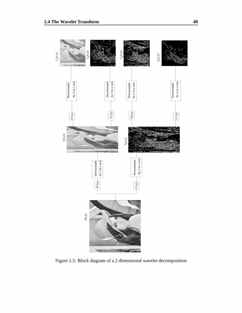
Figure 2.5 shows the process of a 2 dimensional wavelet decomposition. Fig-
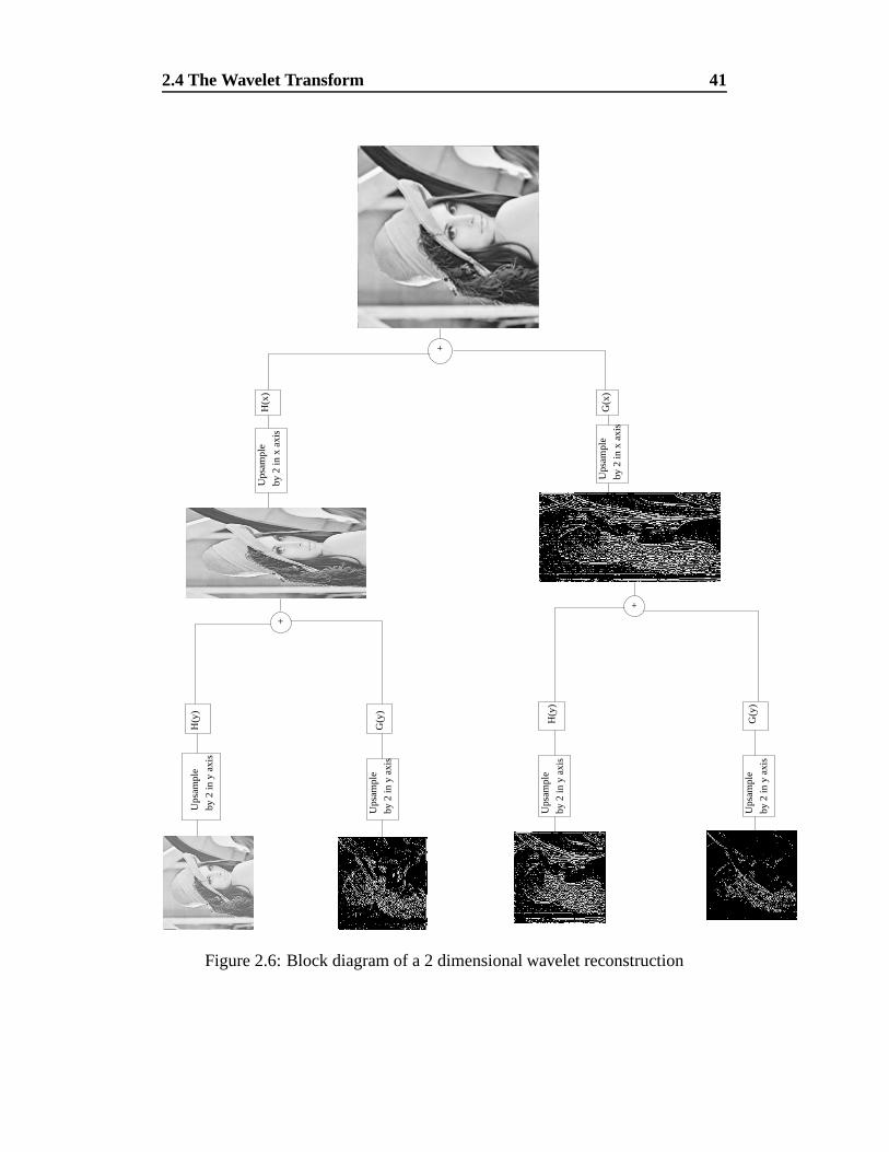
ure 2.6 is the corresponding reconstruction process.
In her landmark paper, Daubechies [Dau88] developed a set of filters for orthonor-
mal, compactly supported wavelets of differing sizes. These particular wavelet
2.4 The Wavelet Transform 40
G’(
x)
H’(
x)
by 2
in x
axi
s
Dow
nsam
ple
by 2
in x
axi
s
Dow
nsam
ple
f(x,
y)
f (x
,y)
f (x
,y)
H
L
H’(
y)
G’(
y)
H’(
y)
G’(
y)D
owns
ampl
e
by 2
in y
axi
s
Dow
nsam
ple
by 2
in y
axi
s
Dow
nsam
ple
by 2
in y
axi
s
Dow
nsam
ple
by 2
in y
axi
s
f (
x,y)
f (
x,y)
f (
x,y)
HH
HL
LL f
(x,
y)L
H
Figure 2.5: Block diagram of a 2 dimensional wavelet decomposition
2.4 The Wavelet Transform 41
Ups
ampl
e
by 2
in y
axi
s
Ups
ampl
e
by 2
in y
axi
s
H(y
)
G(y
)
Ups
ampl
e
by 2
in y
axi
s
Ups
ampl
e
by 2
in y
axi
s
H(y
)
G(y
)
+
Ups
ampl
e
by 2
in x
axi
s
Ups
ampl
e
by 2
in x
axi
s
H(x
)
G(x
)
+
+
Figure 2.6: Block diagram of a 2 dimensional wavelet reconstruction
2.4 The Wavelet Transform 42
bases are ideal for block-wise image processing techniques since the orthonor-
mality condition assures easy computation, while the compact support reduces
the boundary artifacts at block edges. The filters defined in [Dau88] and used
throughout this thesis will be denoted by ����� � or � � where � is the number
of taps of the filter.
It is worth noting here that since the wavelet transform is a bounded linear op-
erator, it preserves the norm on its underlying space. Hence, for the purposes of
image coding, it may be assumed that the � � norm will be preserved across the
wavelet transform. That is, � � � � � � � � � � � � � � � � � � � � � where�
is the
wavelet transform.
2.4.3 Multiresolution Analysis
The notion of a multiresolution analysis is to denote a function� � � � � � � as
the limit of successive approximations of�
. The approximations are smoothed by
successively more concentrated smoothing functions and thus each approximation
is on a different scale or resolution. A multiresolution analysis actually consists
of a family of nested, closed subspaces! � � � � � � � ' � � � ,
� � �
� ! � � � ! �� � ! � � ! � !��� � � (2.15)
such that�� ��
! � � � � � (2.16)
2.4 The Wavelet Transform 43
and �� �
! � � � � � � � (2.17)
and� � ! � � � � �
�� � ! � �� � (2.18)
Define� � � ! � � � ! � . Then
! � � � ! ��� � � . A function� � � � � � � can be
approximated arbitrarily well by projections, � � � , into the subspaces! � ( from
equation 2.17 ). Also, by equation 2.16, as � ��
� , the energy of the projections
� � � becomes arbitrarily small. Now, define
� � � � ����� � �� � � � � �
�
� � (2.19)
Assume the subspace! � is generated by a single function � � � � � � � in the sense
that� � � � � ' � � � � is a Riesz basis of
! � . For a set� � � � to be a Reisz (uncondi-
tional) basis, there must exist � ' � � ' � � � � � � such that
� � � � � � � � �������
��� � � �
� � � �������
�� � � � � � � � (2.20)
for all bi-infinite sequences� � � � � �
� . Then, all the subspaces! � are generated
by the same � in the sense that� ��� � � ' � � � � is a basis of
! � ( by equation 2.18).
Now, as� �
�
� , the Reisz basis functions� �#� � � ' � � � � have decreasing fre-
quency. Therefore, the detail removed by moving from! � to
! � �� must be stored
in the complementary subspace� � . Thus, the multiresolution analysis model of
the wavelet transform decomposition is directly interchangeable with the high-
pass/lowpass model shown in section 2.4.2.
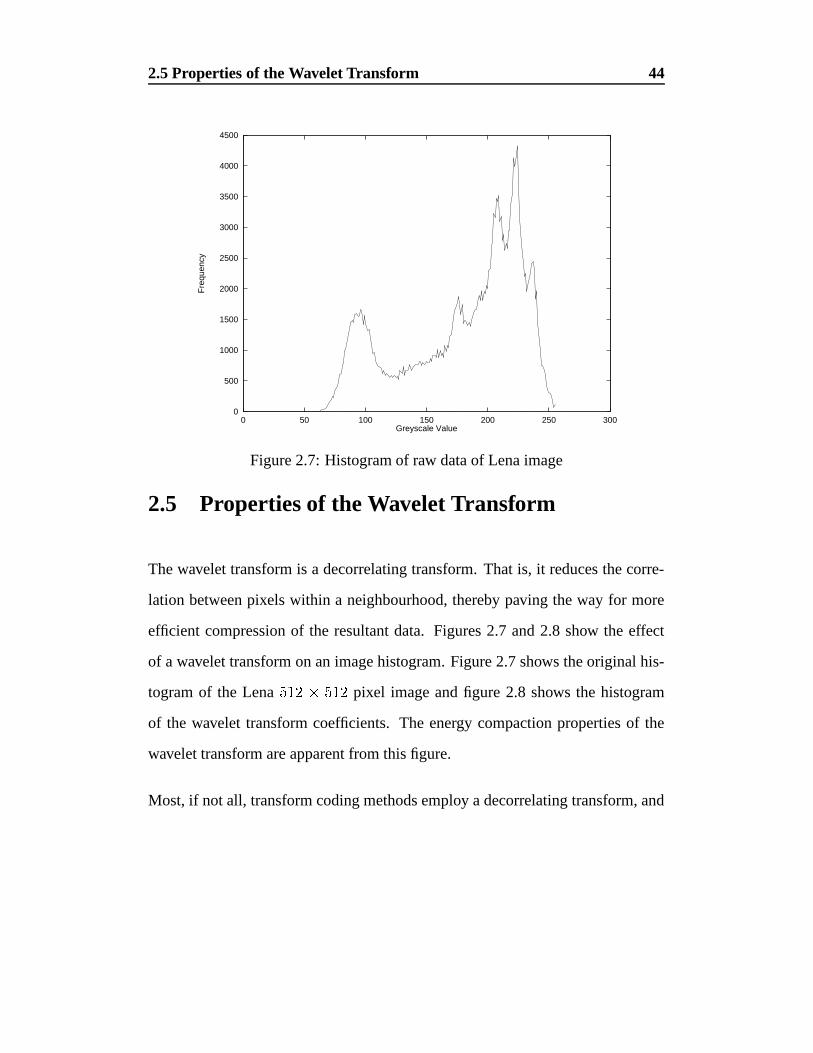
2.5 Properties of the Wavelet Transform 44
0
500
1000
1500
2000
2500
3000
3500
4000
4500
0 50 100 150 200 250 300
Fre
quen
cy
Greyscale Value
Figure 2.7: Histogram of raw data of Lena image
2.5 Properties of the Wavelet Transform
The wavelet transform is a decorrelating transform. That is, it reduces the corre-
lation between pixels within a neighbourhood, thereby paving the way for more
efficient compression of the resultant data. Figures 2.7 and 2.8 show the effect
of a wavelet transform on an image histogram. Figure 2.7 shows the original his-
togram of the Lena����� � ��� �
pixel image and figure 2.8 shows the histogram
of the wavelet transform coefficients. The energy compaction properties of the
wavelet transform are apparent from this figure.
Most, if not all, transform coding methods employ a decorrelating transform, and
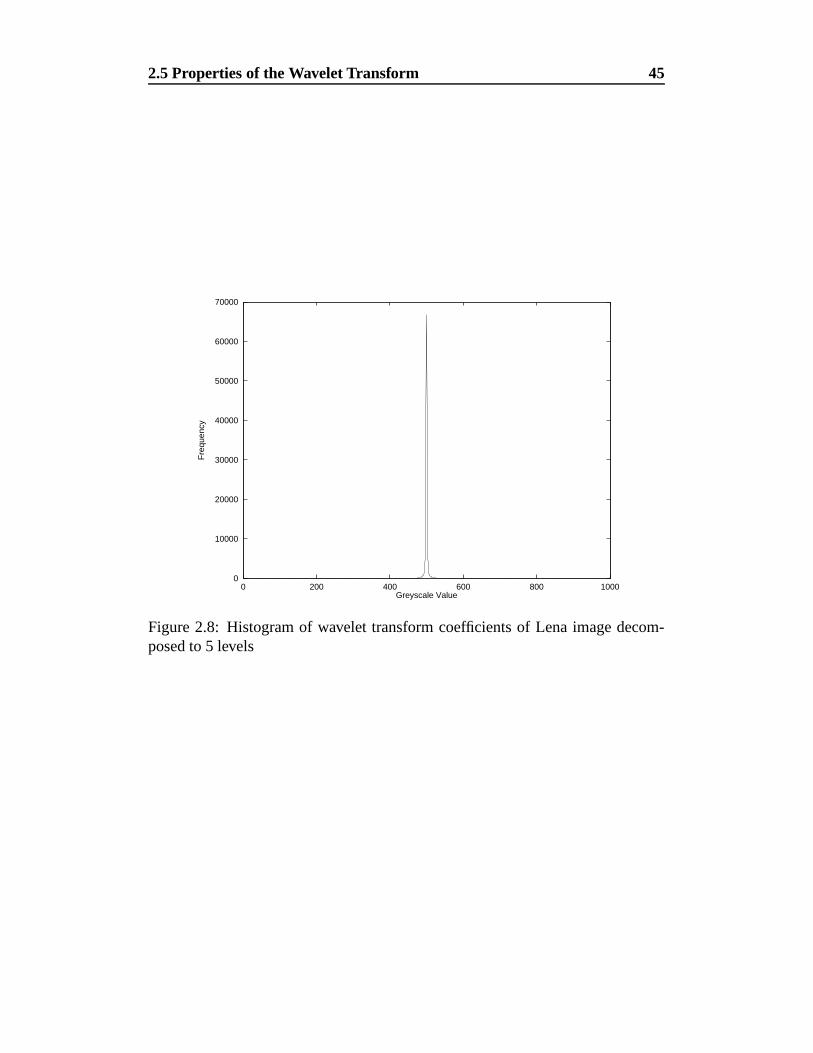
2.5 Properties of the Wavelet Transform 45
0
10000
20000
30000
40000
50000
60000
70000
0 200 400 600 800 1000
Fre
quen
cy
Greyscale Value
Figure 2.8: Histogram of wavelet transform coefficients of Lena image decom-posed to 5 levels
2.6 Wavelet Transform Coding Methods 46
the wavelet transform is very similar in this respect. What the wavelet transform
does, in addition to the decorrelation of the data, is to give a multiresolution rep-
resentation of the data in the horizontal, vertical and diagonal directions ( the pre-
ferred orientations ). Figure 2.9 shows a typical wavelet decomposition to three
levels, shown as absolute value to give a better view of the data.
By inspection, it is obvious that the wavelet transform does indeed attempt to
separate the detail at a given scale into the preferred orientations. However, due
to the restricted number of detail bands the orientation selectivity of the wavelet
transform is not as tight as may be desired. A method for improving the orienta-
tion selectivity will be detailed later. Self-similarity is evident in figure 2.9 - the
wavelet bands at different scales are very similar. This demonstrates the connec-
tion between wavelet and fractal descriptions of image data.
2.6 Wavelet Transform Coding Methods
Wavelet transform coding has been prevalent in research circles since its intro-
duction in [ABMD92]. These authors used a simple separable wavelet decompo-
sition, and then coded the resulting coefficients using a vector quantizer with a
multiresolution codebook, generated from a suitable sample of images. A mul-
tiresolution codebook is an amalgamation of many sub-codebooks. Once an im-
age is decomposed via the wavelet transform, each directional (horizontal, verti-
cal, diagonal) sub-band at each level has a codebook generated for it. This method,
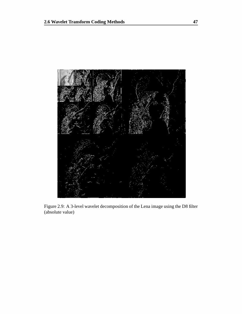
2.6 Wavelet Transform Coding Methods 47
Figure 2.9: A 3-level wavelet decomposition of the Lena image using the D8 filter(absolute value)
2.6 Wavelet Transform Coding Methods 48
it is argued by the authors, results in a more optimal codebook than a global one.
Indeed, it is known that using a global codebook for vector quantization smooths
high frequency features, such as edges and textures. Using a codebook gener-
ated on each individual wavelet sub-band results in vectors that suit the edge arti-
facts encountered there much better. Also, the resulting sub-codebooks are much
smaller and perform better than the global codebook on their particular sub-band.
The authors limit the search for each vector to be coded to the appropriate sub-
codebook. That is, if a vector to be coded is taken from wavelet subband � � ' � �
then only the sub-codebook generated on subband � � ' � � will be searched. The
sub-codebooks are generated and optimized using the Linde-Buzo-Gray method,
described in [LBG80]. Finally, a bit allocation scheme is employed, based on the
relative visual importance of each sub-band. The authors, however, do not con-
centrate on obtaining the lowest possible bit rate. Instead, they provide an insight
into the effects that different filter designs have on the signal-to-noise ratio of a
coded image at a given bit rate.
The benchmark for wavelet transform coding algorithms remains Shapiro’s em-
bedded zerotree method [Sha93]. In this paper, Shapiro presented a new data
structure called the zerotree which is very similar to the classic quadtree structure.
Consider the coefficient tree shown in figure 2.10. The coefficient at the coarsest
scale has children at each finer scale as shown in the figure, creating the quadtree
structure. The zerotree is really a very simple structure, consisting of four symbols
� Zerotree root
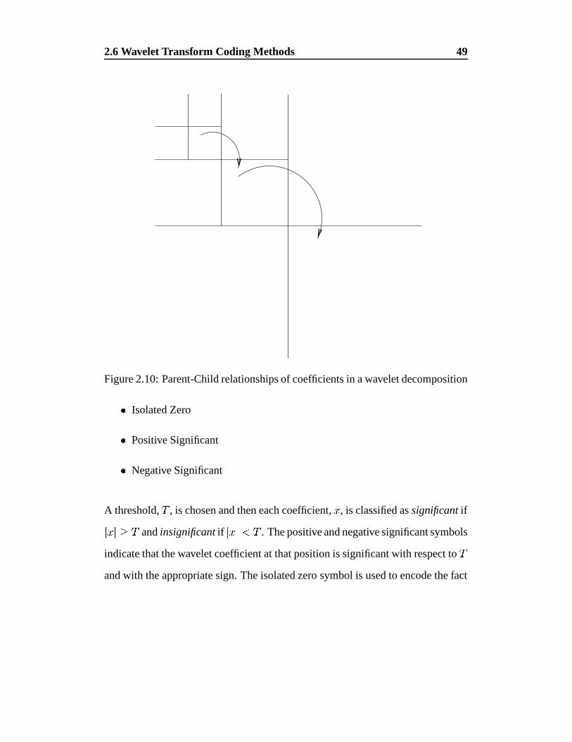
2.6 Wavelet Transform Coding Methods 49
Figure 2.10: Parent-Child relationships of coefficients in a wavelet decomposition
� Isolated Zero
� Positive Significant
� Negative Significant
A threshold,�
, is chosen and then each coefficient, � , is classified as significant if
� � � � �and insignificant if � � � � �
. The positive and negative significant symbols
indicate that the wavelet coefficient at that position is significant with respect to�
and with the appropriate sign. The isolated zero symbol is used to encode the fact
2.7 Summary 50
that the current wavelet coefficient is insignificant, although some of its children
are not. The zerotree root symbol means that this coefficient and all its children
are insignificant. Obviously, at the bottom level of the wavelet decomposition (the
highest frequency bands), a coefficient has no children. In this case, the zerotree
root symbol is not used, and the semantics of the significant symbols change.
The alphabet for encoding the map is reduced to two symbols; namely significant
and insignificant. The zerotree is used to code a significance map of wavelet
coefficients. Only coefficients with a non-zero entry in the significance map are
actually sent. This can reduce the bitrate immensely if the wavelet decomposition
significance map contains many zerotree root symbols. Shapiro’s zerotree encoder
exploits a basic notion of image self-similarity, much as standard fractal coding
does. However, Shapiro’s method concentrates on the inter-level similarity of
insignificant data. This, in turn, represents the insignificant data at different scales
in the original image, hence the self-similarity argument. In the next chapter, the
connection between wavelets and self-similarity will be exploited in the design of
a still image coder.
2.7 Summary
This chapter has introduced the concept of fractal image coding using iterated
functions systems. The main problem, from an image coding standpoint, is that it
has been shown that it is impossible for a fractal image coder to achieve perfect
reconstruction of an arbitrary signal. An analysis of the basis generated by the

2.7 Summary 51
fractal method related the basis to that generated by the wavelet transform using
quadrature mirror filters. Comparisons drawn between fractal and wavelet meth-
ods demonstrate the multiresolution nature of both. Combining the two methods
into an image coding algorithm is the obvious next step.
Chapter 3
Exploiting Fractal Compression inthe Wavelet Domain
Both fractal block coding and wavelet transform coding rely on the symmetries
inherent in image data. As discussed in the previous chapter, the wavelet basis
is a more natural basis for the fractal method than the one generated by dyadic
downsampling and the addition of constant blocks. It seems, therefore, natural to
attempt to unify the two disparate strategies.
3.1 A predictive wavelet transform coder
The method presented here can be seen as a predictive coder, operating in the
wavelet domain. Blocks of data representing larger scales are used to predict those
at smaller scales [Tod89]. The method is a recursive one, performed one wavelet
level at a time, in which the preferred orientation bands are treated together.
52
3.1 A predictive wavelet transform coder 53
3.1.1 Algorithm Description
The image to be coded is decomposed by the wavelet transform to a given level,
say�, known as the base level. The first level to be approximated, called the do-
main level, is then� � �
. Then, the range level is the level from which the domain
level shall be approximated, that is� � � � � . The construction of the relevant lev-
els is shown in Figure 3.1, where� � � ' � � � ' � �� . Levels from
�through
�are
quantized using a linear quantizer for the highpass coefficients. A separate quan-
tizer is used for the lowpass coefficients at the highest level, since the statistics
of the data are sufficiently different. In the spirit of equation 2.13, the quantized
approximation is used as the range level of coefficients to reduce errors at the de-
coder. Each of the bands in the domain level is partitioned into non-overlapping
domain blocks. Let� � ���� � , � � ���� � and
� � ���� � be the domain blocks from each
subband. For each domain block set� � ���� ' � ���� ' � ���� � , a corresponding range
block set� � ���� ' � ���� ' � ���� � must be found which minimizes the error
� � � � �����
������ � � � � � ����
�
������ � � � � � ����
�
������ � � (3.1)
where���� � � � � � �
�
�� �� � (3.2)
�� � is a normalised range block,
� � � � �� ���� ' � ���� � � �� ���� ' � ���� � � �� ���� ' � ���� � �� ���� ' �� ���� � � �� ���� ' �� ���� � � �� ���� ' �� ���� (3.3)
and� � � � is the dihedral group of the square, i.e. combinations of rotations by
�
�
and flips around the mid-point axes. Hence, the blocks from the three subbands
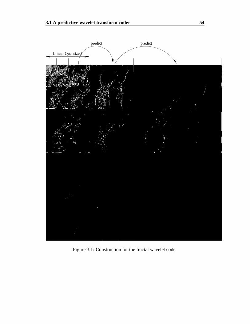
3.1 A predictive wavelet transform coder 54
Linear Quantized
predictpredict
Figure 3.1: Construction for the fractal wavelet coder
3.1 A predictive wavelet transform coder 55
are scaled by the same factor.
Since an orthogonal wavelet transform is used, the subbands are all orthogonal.
Hence, no iteration of the fractal block maps is required, since any errors will be
orthogonal to the approximation. Since there will be no iteration of the maps in
the decoding process, the value of � � is unconstrained. Given a domain block size
� � and search radius � � , define the search region as the subset of the subband�
given by � ��
� � � � ' � � � � � � � � ��
� � � � ' � � � � � � � � � �. A spiral search from
the centre of the search region is used to address the range blocks. Obviously, a
method which performs no searching is also possible. This method constrains the
maps so that each range block� �� (
� � ����� ' � � ' � � � ) is in the same relative
position, but in different subbands. The reasoning behind this is that if two blocks
are similar, then their horizontal, vertical and diagonal components must also be
similar.
This process is then repeated on successive levels of the wavelet decomposition.
The approximation of the domain level generated by the coder thus becomes the
range coefficients for the next level. Separate affine map coefficients are generated
between levels, up to level 1.
3.1.2 Handling Prediction Errors
The coder attempts to extrapolate a block in the range level to a block in the
domain level in each subband. However, if a range block which provides an ade-
3.1 A predictive wavelet transform coder 56
quate approximation cannot be found, the block error will be large. To overcome
this, block projection is performed after the inter-level prediction to reduce er-
rors, in the same vein as Huang and Gharavi-Alkhansari [GAH94]. This method,
however, is simpler, since it is based on the Karhunen-Loeve transform. Dur-
ing a training phase, each error block arising from the prediction across levels is
stored, along with all its symmetries. The process is repeated across a range of
images and the symmetrized error vectors are accumulated. The Karhunen-Loeve
transform is then applied to the symmetrized error vectors produced during the
prediction phases, producing an orthonormal basis of the error population. Since
the population contains symmetrized vectors, the resultant basis vectors are all
symmetric. Prediction errors are now handled simply by projecting any errors
onto the orthonormal basis generated from the Karhunen-Loeve transform.
3.1.3 The Karhunen-Loeve transform
Consider a population of random vectors of the form
� �� �
� ...� "
� ��� (3.4)
Defining � $ � � ����� as the mean of � and the covariance matrix
�%$ � � � ����
� $ � � ��
� $ ����� (3.5)
where�
denotes vector transposition and� ��� denotes expectation. For � vectors
taken from a random population, the mean vector and covariance matrix can be
3.1 A predictive wavelet transform coder 57
approximated by the sample averages
� $ � �
�
��� �
� � (3.6)
and
�%$ � �
�
��� �
� � � � � � � $ � � $ (3.7)
Now, �%$ is a real, symmetric � � � matrix. As such, it is guaranteed that a set of �orthonormal eigenvectors is always calculable [Ner69]. Order the eigenvalues of
�%$ ,� � � � , in decreasing value and define row � of a matrix, � , to be the eigenvector
associated with eigenvalue� � . Then, the Karhunen-Loeve transform is defined
([GW92]) as
� � � � ��
� $ � (3.8)
The vectors � are then uncorrelated and have zero mean. However, for this appli-
cation, only the eigenvectors of the covariance matrix, � $ are required, since they
form an orthonormal basis of the underlying population. Threshold coding using
a� � �
KLT is used to code the prediction errors.
3.1.4 Entropy Coding
The parameter sets that describe the blockwise maps and the basis projection co-
efficients are linearly quantized and entropy coded. A rate value determines how
many bins the quantizer uses and how many symbols the arithmetic coder can
encode. Figure 3.2 shows a block diagram of the hybrid coder.
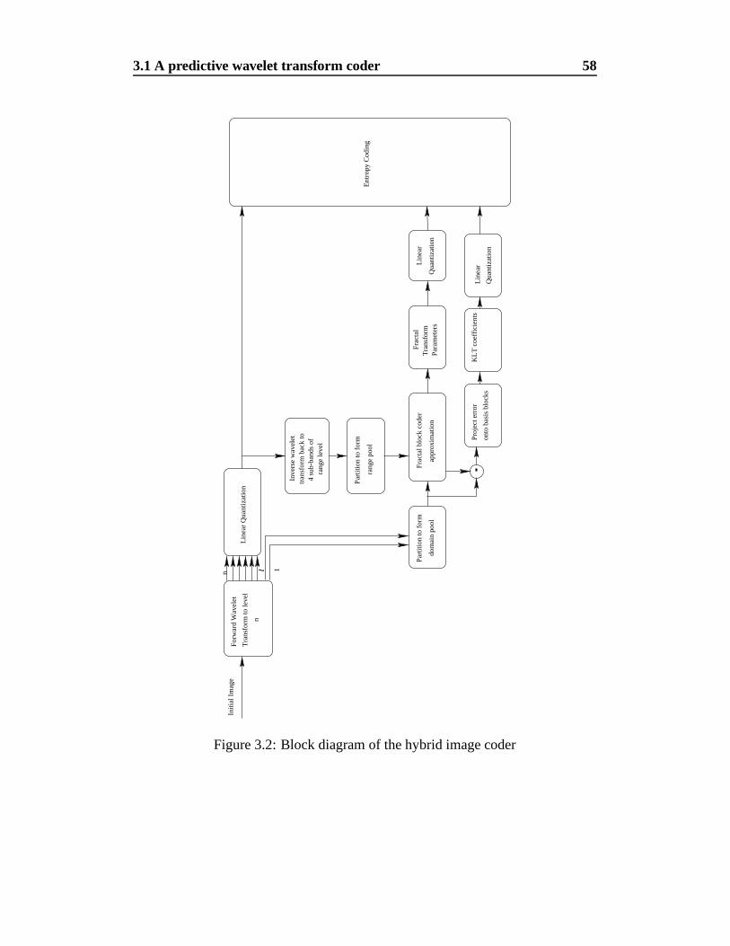
3.1 A predictive wavelet transform coder 58
nF
orw
ard
Wav
elet
Tra
nsfo
rm to
leve
lL
inea
r Q
uant
izat
ion
Init
ial I
mag
e
Par
titi
on to
for
m
rang
e po
ol
Fra
ctal
T
rans
form
Par
amet
ers
Lin
ear
Qua
ntiz
atio
n
n
Pro
ject
err
or
onto
bas
is b
lock
s
KL
T c
oeff
icie
nts
Lin
ear
Qua
ntiz
atio
n
Par
titi
on to
for
m
dom
ain
pool
Fra
ctal
blo
ck c
oder
appr
oxim
atio
n
1
Inve
rse
wav
elet
tr
ansf
orm
bac
k to
4 su
b-ba
nds
ofra
nge
leve
l
Ent
ropy
Cod
ing
l
Figure 3.2: Block diagram of the hybrid image coder
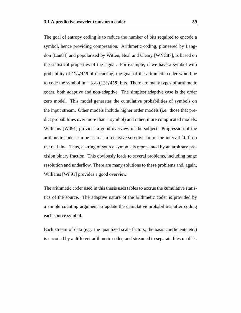
3.1 A predictive wavelet transform coder 59
The goal of entropy coding is to reduce the number of bits required to encode a
symbol, hence providing compression. Arithmetic coding, pioneered by Lang-
don [Lan84] and popularised by Witten, Neal and Cleary [WNC87], is based on
the statistical properties of the signal. For example, if we have a symbol with
probability of��� � � ��� of occurring, the goal of the arithmetic coder would be
to code the symbol in � � ��� ��� � � ��� � bits. There are many types of arithmetic
coder, both adaptive and non-adaptive. The simplest adaptive case is the order
zero model. This model generates the cumulative probabilities of symbols on
the input stream. Other models include higher order models (i.e. those that pre-
dict probabilities over more than 1 symbol) and other, more complicated models.
Williams [Wil91] provides a good overview of the subject. Progression of the
arithmetic coder can be seen as a recursive sub-division of the interval � ' � �
on
the real line. Thus, a string of source symbols is represented by an arbitrary pre-
cision binary fraction. This obviously leads to several problems, including range
resolution and underflow. There are many solutions to these problems and, again,
Williams [Wil91] provides a good overview.
The arithmetic coder used in this thesis uses tables to accrue the cumulative statis-
tics of the source. The adaptive nature of the arithmetic coder is provided by
a simple counting argument to update the cumulative probabilities after coding
each source symbol.
Each stream of data (e.g. the quantized scale factors, the basis coefficients etc.)
is encoded by a different arithmetic coder, and streamed to separate files on disk.

3.2 Orientation in Wavelet Subbands 60
This allows the arithmetic coders more accurately to model the statistics of each
stream and allows for simple analysis of the resultant files.
3.1.5 Reconstruction
Reconstruction proceeds much the same as for conventional fractal coding. The
lowpass and base level of the wavelet coefficients are decoded and the first set of
fractal block maps is then applied to the base level. Any basis projection coeffi-
cients are applied block-wise. The reconstructed level is then used as the domain
for the next set of affine transforms. Note that, unlike conventional fractal com-
pression, the fractal block maps are not iterated. An inverse wavelet transform
from the base level reconstructs the original image.
3.2 Orientation in Wavelet Subbands
Assume that the wavelet decomposition has been performed on an image to a
specific level. Label the transform coefficient bands���� ,
���� ,
���� and
���� at that
level. Then the orientation of the pixel at position ��� ' ��� in the LL band of the
level below is approximated by
� � ' ��� � ��� ��� � �� � � � �
��� � � ' ��� � ���� � $ � ��
� � ���� ��� ' �#� � ����� � $ � �
�
� ���� � � ' ��� � ����� � $ � �
� ��
� ���� ��� ' �#� � ����� � $ � �
� �
�� �
(3.9)
The orientation estimate can be used further to reduce the size of the pool to be
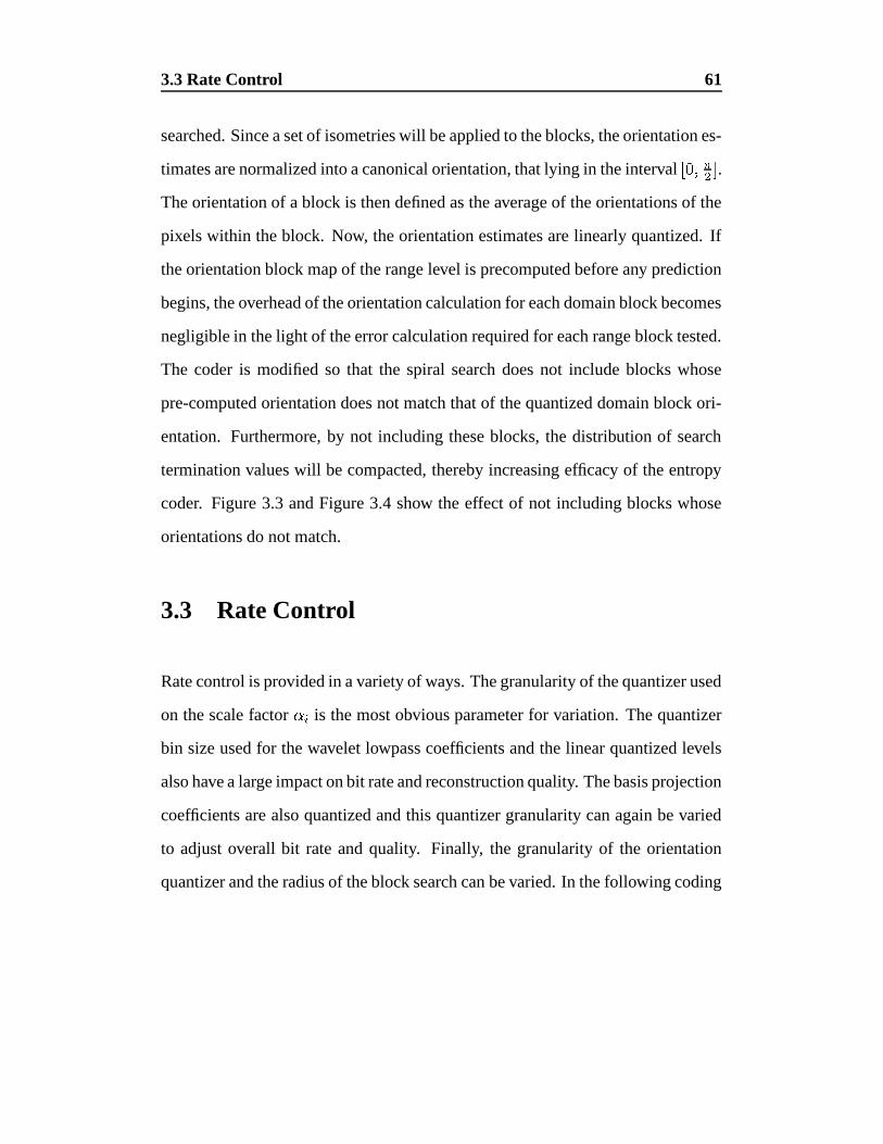
3.3 Rate Control 61
searched. Since a set of isometries will be applied to the blocks, the orientation es-
timates are normalized into a canonical orientation, that lying in the interval � ' ���.
The orientation of a block is then defined as the average of the orientations of the
pixels within the block. Now, the orientation estimates are linearly quantized. If
the orientation block map of the range level is precomputed before any prediction
begins, the overhead of the orientation calculation for each domain block becomes
negligible in the light of the error calculation required for each range block tested.
The coder is modified so that the spiral search does not include blocks whose
pre-computed orientation does not match that of the quantized domain block ori-
entation. Furthermore, by not including these blocks, the distribution of search
termination values will be compacted, thereby increasing efficacy of the entropy
coder. Figure 3.3 and Figure 3.4 show the effect of not including blocks whose
orientations do not match.
3.3 Rate Control
Rate control is provided in a variety of ways. The granularity of the quantizer used
on the scale factor � � is the most obvious parameter for variation. The quantizer
bin size used for the wavelet lowpass coefficients and the linear quantized levels
also have a large impact on bit rate and reconstruction quality. The basis projection
coefficients are also quantized and this quantizer granularity can again be varied
to adjust overall bit rate and quality. Finally, the granularity of the orientation
quantizer and the radius of the block search can be varied. In the following coding
3.3 Rate Control 62
0
20
40
60
80
100
120
140
160
180
0 50 100 150 200 250
Fre
quen
cy
Path Length
Figure 3.3: Distribution of path positions when block orientations are not matched
0
50
100
150
200
250
0 50 100 150 200 250
Fre
quen
cy
Path Length
Figure 3.4: Distribution of path positions when block orientations are matched
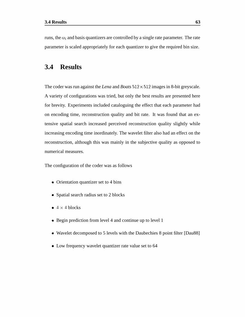
3.4 Results 63
runs, the � � and basis quantizers are controlled by a single rate parameter. The rate
parameter is scaled appropriately for each quantizer to give the required bin size.
3.4 Results
The coder was run against the Lena and Boats����� � �����
images in 8-bit greyscale.
A variety of configurations was tried, but only the best results are presented here
for brevity. Experiments included cataloguing the effect that each parameter had
on encoding time, reconstruction quality and bit rate. It was found that an ex-
tensive spatial search increased perceived reconstruction quality slightly while
increasing encoding time inordinately. The wavelet filter also had an effect on the
reconstruction, although this was mainly in the subjective quality as opposed to
numerical measures.
The configuration of the coder was as follows
� Orientation quantizer set to 4 bins
� Spatial search radius set to 2 blocks
�� � �
blocks
� Begin prediction from level 4 and continue up to level 1
� Wavelet decomposed to 5 levels with the Daubechies 8 point filter [Dau88]
� Low frequency wavelet quantizer rate value set to 64
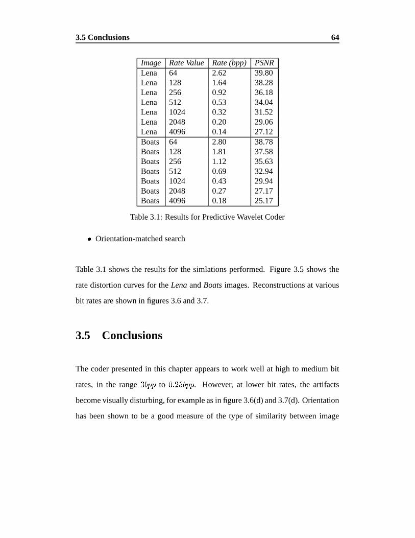
3.5 Conclusions 64
Image Rate Value Rate (bpp) PSNRLena 64 2.62 39.80Lena 128 1.64 38.28Lena 256 0.92 36.18Lena 512 0.53 34.04Lena 1024 0.32 31.52Lena 2048 0.20 29.06Lena 4096 0.14 27.12Boats 64 2.80 38.78Boats 128 1.81 37.58Boats 256 1.12 35.63Boats 512 0.69 32.94Boats 1024 0.43 29.94Boats 2048 0.27 27.17Boats 4096 0.18 25.17
Table 3.1: Results for Predictive Wavelet Coder
� Orientation-matched search
Table 3.1 shows the results for the simlations performed. Figure 3.5 shows the
rate distortion curves for the Lena and Boats images. Reconstructions at various
bit rates are shown in figures 3.6 and 3.7.
3.5 Conclusions
The coder presented in this chapter appears to work well at high to medium bit
rates, in the range �����
to� � � � ����� . However, at lower bit rates, the artifacts
become visually disturbing, for example as in figure 3.6(d) and 3.7(d). Orientation
has been shown to be a good measure of the type of similarity between image
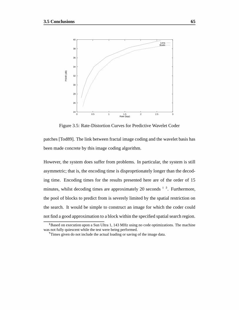
3.5 Conclusions 65
24
26
28
30
32
34
36
38
40
0 0.5 1 1.5 2 2.5 3
PS
NR
(dB
)
Rate (bpp)
LenaBoats
Figure 3.5: Rate-Distortion Curves for Predictive Wavelet Coder
patches [Tod89]. The link between fractal image coding and the wavelet basis has
been made concrete by this image coding algorithm.
However, the system does suffer from problems. In particular, the system is still
asymmetric; that is, the encoding time is disproprtionately longer than the decod-
ing time. Encoding times for the results presented here are of the order of 15
minutes, whilst decoding times are approximately 20 seconds � . Furthermore,
the pool of blocks to predict from is severely limited by the spatial restriction on
the search. It would be simple to construct an image for which the coder could
not find a good approximation to a block within the specified spatial search region.�Based on execution upon a Sun Ultra 1, 143 MHz using no code optimizations. The machine
was not fully quiescent while the test were being performed.�Times given do not include the actual loading or saving of the image data.
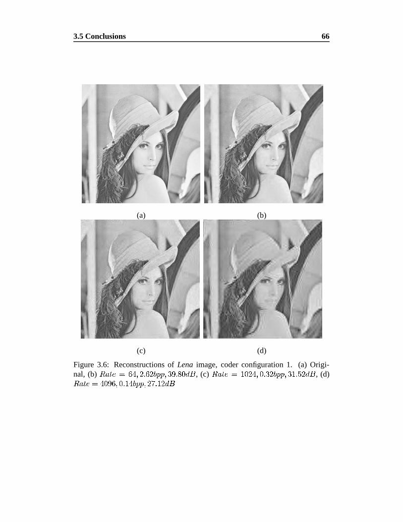
3.5 Conclusions 66
(a) (b)
(c) (d)
Figure 3.6: Reconstructions of Lena image, coder configuration 1. (a) Origi-nal, (b)
� / � � � ��� ' � � � � ����� ' � � � � , (c)� / � � � ��� � � ' � � � ����� ' � � � � � , (d)� / � � � � � � � ' � � � � ����� ' � � � � � �
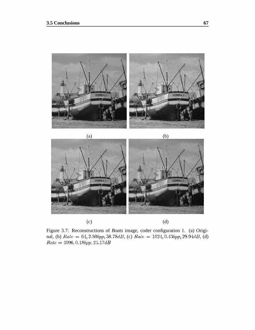
3.5 Conclusions 67
(a) (b)
(c) (d)
Figure 3.7: Reconstructions of Boats image, coder configuration 1. (a) Origi-nal, (b)
� / � � � ��� ' � � ������� ' � � � � , (c)� / � � � ��� � � ' � � � ����� ' � � � � � � , (d)� / � � � � � � � ' � � � ����� ' � � � � � �

3.5 Conclusions 68
In this case, the coder would degenerate to a simple basis projection and would
obviously perform poorly.
Chapter 4
Predictive Wavelet Image CodingUsing an Oriented Transform
As mentioned in section 2.5, the wavelet transform attempts to group image data
into bands of oriented features at each scale. From the previous chapter, ori-
entation is important in still image coding applications. The frequency domain
tessellation in figure 4.1 shows the split into frequency bands provided by the
conventional wavelet transform. The predictive coding scheme presented in chap-
ter 3 requires a search of some sort in order to find the best block from which to
predict. This search could be restricted without adversely affecting reconstruction
quality by limiting the search to similar blocks. The metric of similarity could
be arbitrarily defined, but grouping the blocks by orientation is a natural option.
However, the conventional two dimensional wavelet transform does not provide
sufficient resolution in orientation for this to be feasible.
69
4.1 An Oriented Wavelet Transform 70
4.1 An Oriented Wavelet Transform
In order to increase the orientation selectivity of the transform, it would be use-
ful to increase the number of high-pass bands that the wavelet transform creates
[CMW] [RV93]. This would, in turn, offer greater orientation selectivity within
each band. Wilson and Spann [WS88] presented an invertible multiresolution
transform which provides six orthogonal bandpass features at each scale. This
was presented in the framework of image segmentation, where reconstruction is
not important. Obviously, for image coding applications, perfect or near-perfect
reconstruction is generally required. Treil, Mallat and Bajcsy [TMB89] present a
slightly modified two dimensional dyadic wavelet decomposition in which there
are four highpass bands. Consider the frequency domain tessellation shown in
figure 4.1. This figure shows how the frequency spectrum is split by using QMF
wavelet transform filters. The band � is the lowpass band while the bands� ' � � � '
are the highpass bands in each preferred orientation. In [TMB89] the authors split
the diagonal oriented band (3) into two. The split of the band is denoted by the
‘!’ characters. This provides a small increase in the orientation selectivity of the
transform.
For the purposes of image compression, orthogonal wavelets are the preferred
analysis tool since the wavelet sub-bands are then orthogonal. Obviously any
orientation selectivity increasing modification should attempt to preserve as many
desirable properties of the orthogonal wavelet transform as possible. The most
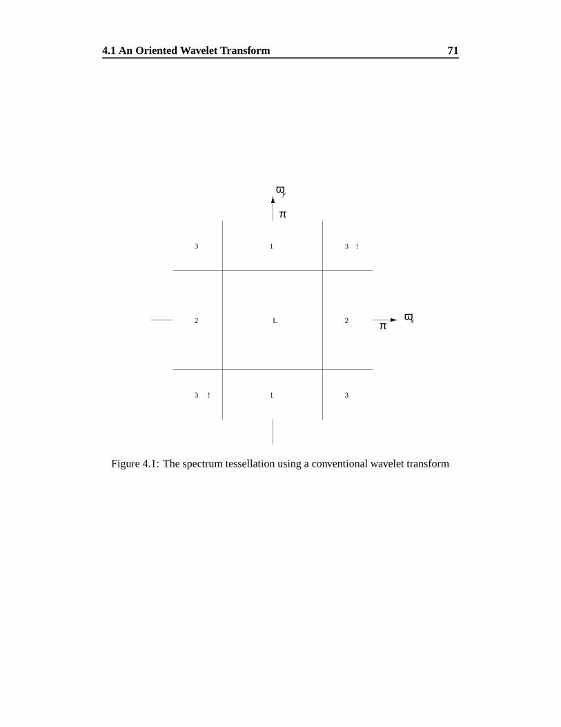
4.1 An Oriented Wavelet Transform 71
ωx
ωy
π
π
1 3 !3
3 ! 3
2 L 2
1
Figure 4.1: The spectrum tessellation using a conventional wavelet transform
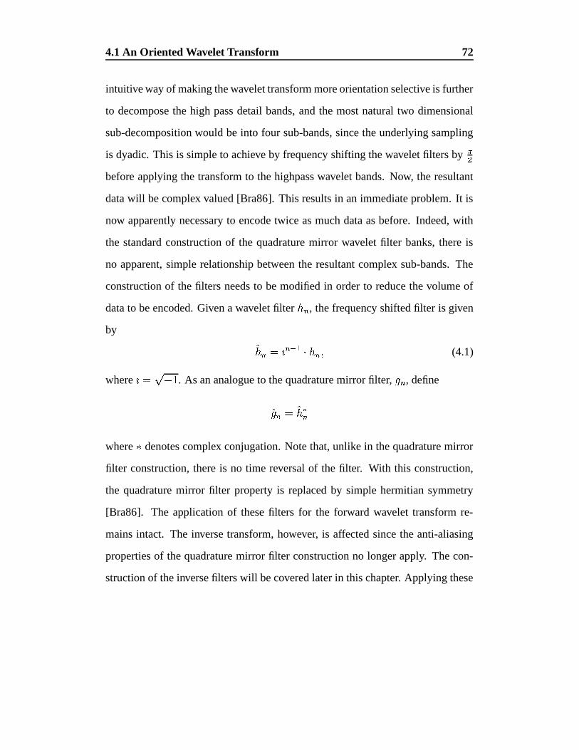
4.1 An Oriented Wavelet Transform 72
intuitive way of making the wavelet transform more orientation selective is further
to decompose the high pass detail bands, and the most natural two dimensional
sub-decomposition would be into four sub-bands, since the underlying sampling
is dyadic. This is simple to achieve by frequency shifting the wavelet filters by�
�
before applying the transform to the highpass wavelet bands. Now, the resultant
data will be complex valued [Bra86]. This results in an immediate problem. It is
now apparently necessary to encode twice as much data as before. Indeed, with
the standard construction of the quadrature mirror wavelet filter banks, there is
no apparent, simple relationship between the resultant complex sub-bands. The
construction of the filters needs to be modified in order to reduce the volume of
data to be encoded. Given a wavelet filter& "
, the frequency shifted filter is given
by�& " � �
" ���
& " '(4.1)
where � ���
�. As an analogue to the quadrature mirror filter,
( ", define
�( " � �& �"
where � denotes complex conjugation. Note that, unlike in the quadrature mirror
filter construction, there is no time reversal of the filter. With this construction,
the quadrature mirror filter property is replaced by simple hermitian symmetry
[Bra86]. The application of these filters for the forward wavelet transform re-
mains intact. The inverse transform, however, is affected since the anti-aliasing
properties of the quadrature mirror filter construction no longer apply. The con-
struction of the inverse filters will be covered later in this chapter. Applying these
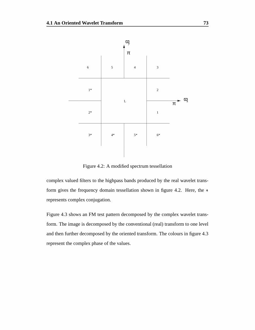
4.1 An Oriented Wavelet Transform 73
ωx
ωy
π
πL
1*
5
4*
2
4
5*
12*
6
6*
3
3*
Figure 4.2: A modified spectrum tessellation
complex valued filters to the highpass bands produced by the real wavelet trans-
form gives the frequency domain tessellation shown in figure 4.2. Here, the �
represents complex conjugation.
Figure 4.3 shows an FM test pattern decomposed by the complex wavelet trans-
form. The image is decomposed by the conventional (real) transform to one level
and then further decomposed by the oriented transform. The colours in figure 4.3
represent the complex phase of the values.
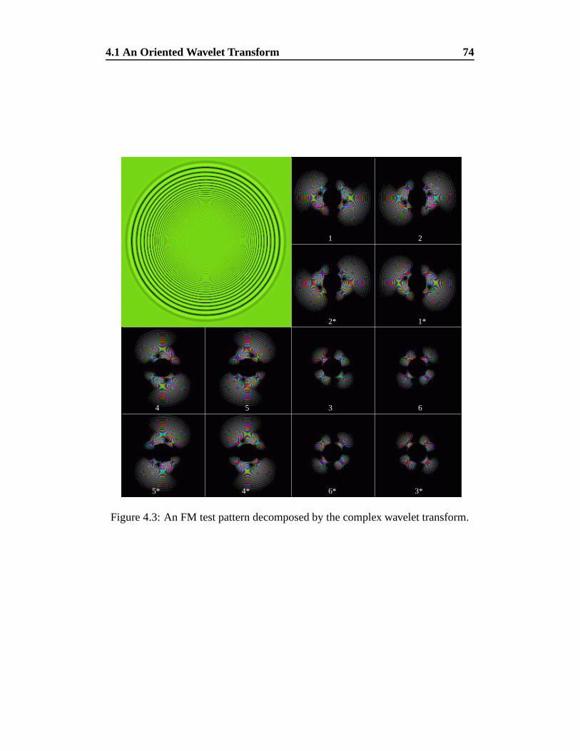
4.1 An Oriented Wavelet Transform 74
21
2* 1*
3 6
6* 3*
54
5* 4*
Figure 4.3: An FM test pattern decomposed by the complex wavelet transform.
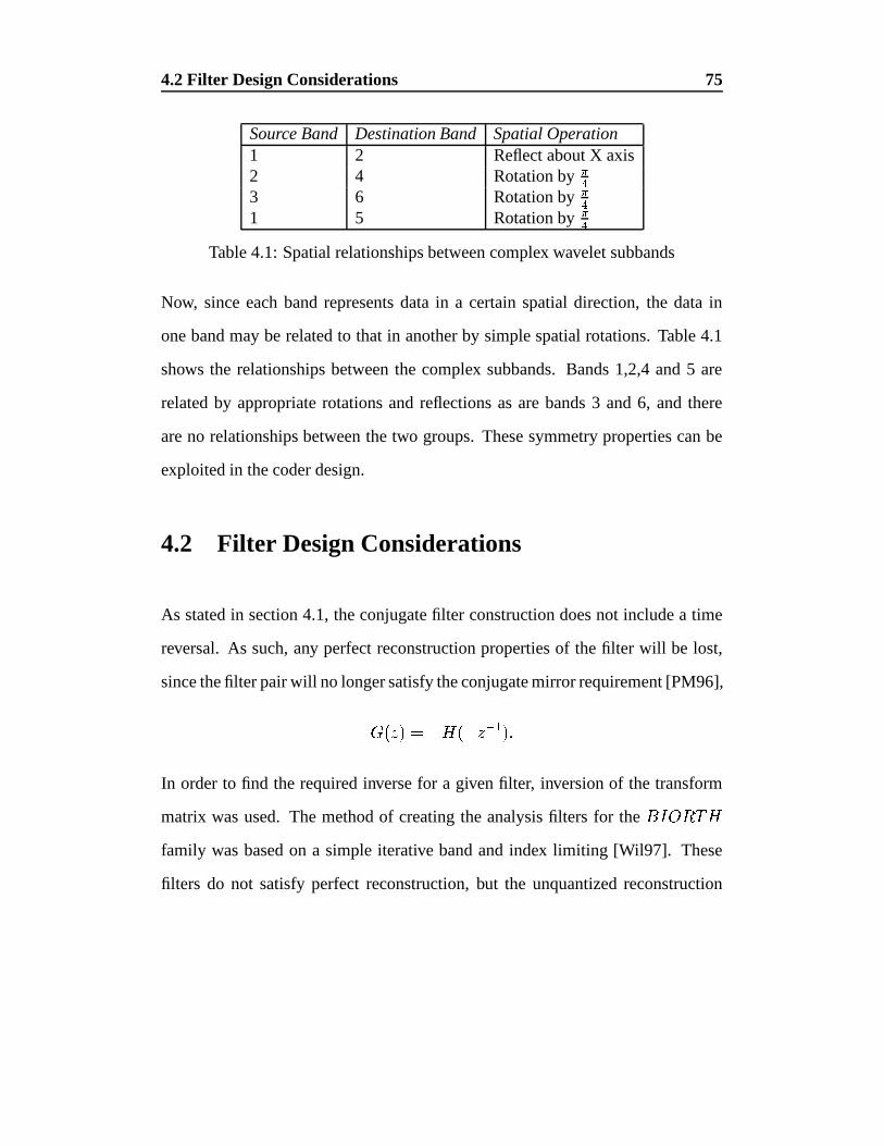
4.2 Filter Design Considerations 75
Source Band Destination Band Spatial Operation1 2 Reflect about X axis2 4 Rotation by
�
�
3 6 Rotation by�
�
1 5 Rotation by�
�
Table 4.1: Spatial relationships between complex wavelet subbands
Now, since each band represents data in a certain spatial direction, the data in
one band may be related to that in another by simple spatial rotations. Table 4.1
shows the relationships between the complex subbands. Bands 1,2,4 and 5 are
related by appropriate rotations and reflections as are bands 3 and 6, and there
are no relationships between the two groups. These symmetry properties can be
exploited in the coder design.
4.2 Filter Design Considerations
As stated in section 4.1, the conjugate filter construction does not include a time
reversal. As such, any perfect reconstruction properties of the filter will be lost,
since the filter pair will no longer satisfy the conjugate mirror requirement [PM96],
� � , � ��
� ��
, �� � �
In order to find the required inverse for a given filter, inversion of the transform
matrix was used. The method of creating the analysis filters for the � � � �
family was based on a simple iterative band and index limiting [Wil97]. These
filters do not satisfy perfect reconstruction, but the unquantized reconstruction
4.3 A Tree Structured Vector Quantizer 76
error is vanishingly small when compared to any coding errors. For reference,
the filters detailed in tables 4.2, 4.3, 4.4 and 4.5 have been produced for use with
the modified conjugate construction and are used throughout the remainder of this
work. Note that the coefficients are presented before the filter has been shifted by�
� as in equation 4.1.
Note that the filters BIORTH610, BIORTH1810 and BIORTH1022 all have sym-
metric analysis filters. This should improve their performance around edges and
reduce ringing artifacts. However, the filter � � � � � ��� analysis filter is
longer than the synthesis filter, which may introduce undesirable visual artifacts
in reconstruction.
4.3 A Tree Structured Vector Quantizer
The block coding algorithm presented in the previous chapter is much less com-
putationally intensive than conventional fractal compression. However, the block
search is restricted in order to increase speed, reducing the pool of available vec-
tors. Furthermore, performing a mean square error test on each block is restrictive
and a simpler, less expensive method would be preferable. In effect, the domain
block pool is simply a set of vectors, which has to be searched to identify the
nearest one to each range block. In other words, it is vector quantization (VQ).
Building a history of previously encoded blocks should also reduce reconstruc-
tion error, since the coder is given a more richly populated vector space to predict
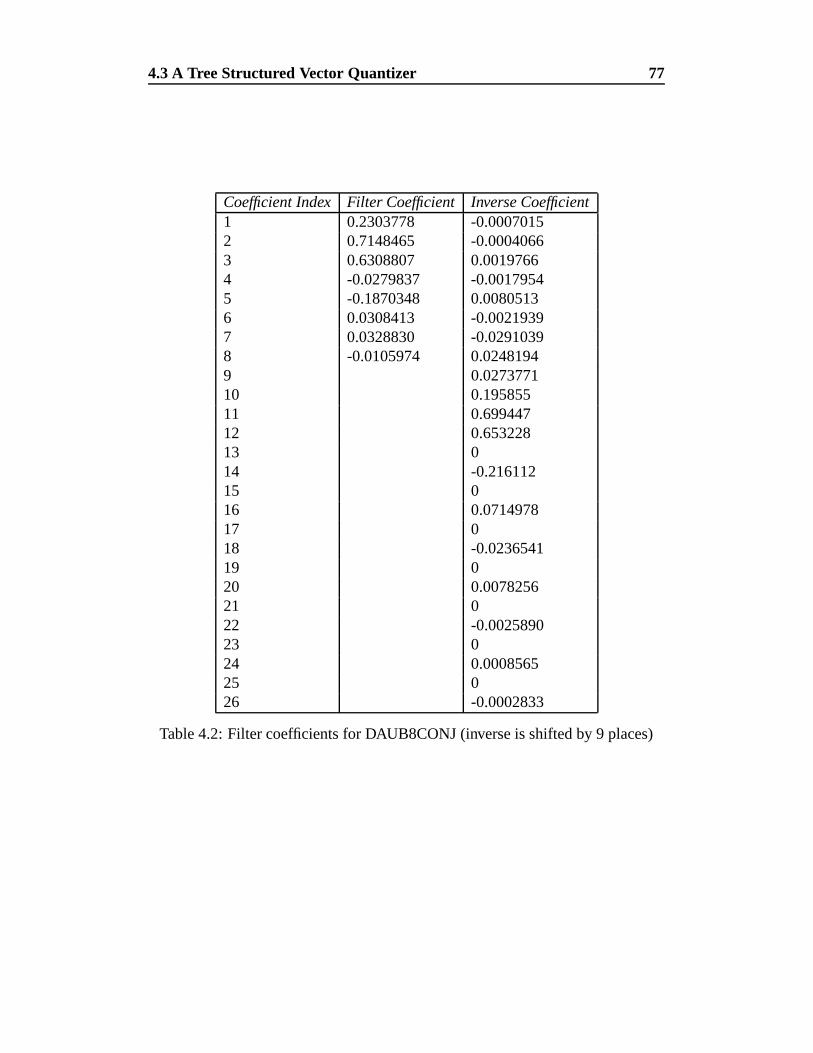
4.3 A Tree Structured Vector Quantizer 77
Coefficient Index Filter Coefficient Inverse Coefficient1 0.2303778 -0.00070152 0.7148465 -0.00040663 0.6308807 0.00197664 -0.0279837 -0.00179545 -0.1870348 0.00805136 0.0308413 -0.00219397 0.0328830 -0.02910398 -0.0105974 0.02481949 0.027377110 0.19585511 0.69944712 0.65322813 014 -0.21611215 016 0.071497817 018 -0.023654119 020 0.007825621 022 -0.002589023 024 0.000856525 026 -0.0002833
Table 4.2: Filter coefficients for DAUB8CONJ (inverse is shifted by 9 places)
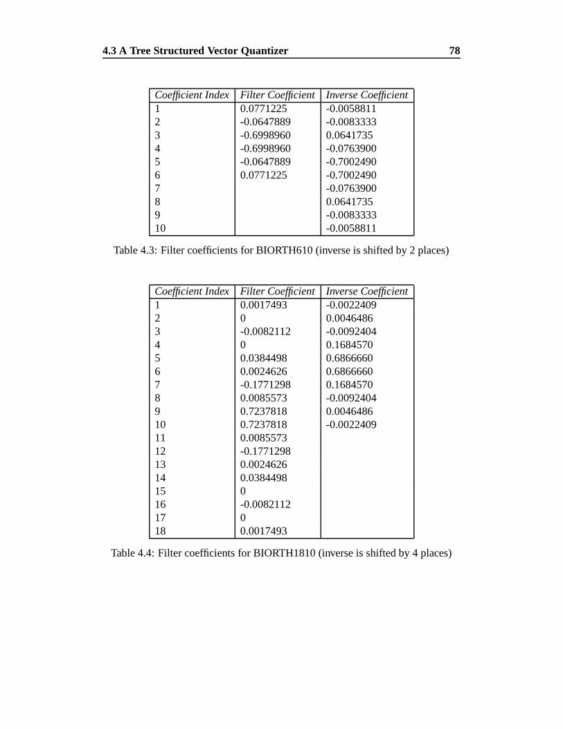
4.3 A Tree Structured Vector Quantizer 78
Coefficient Index Filter Coefficient Inverse Coefficient1 0.0771225 -0.00588112 -0.0647889 -0.00833333 -0.6998960 0.06417354 -0.6998960 -0.07639005 -0.0647889 -0.70024906 0.0771225 -0.70024907 -0.07639008 0.06417359 -0.008333310 -0.0058811
Table 4.3: Filter coefficients for BIORTH610 (inverse is shifted by 2 places)
Coefficient Index Filter Coefficient Inverse Coefficient1 0.0017493 -0.00224092 0 0.00464863 -0.0082112 -0.00924044 0 0.16845705 0.0384498 0.68666606 0.0024626 0.68666607 -0.1771298 0.16845708 0.0085573 -0.00924049 0.7237818 0.004648610 0.7237818 -0.002240911 0.008557312 -0.177129813 0.002462614 0.038449815 016 -0.008211217 018 0.0017493
Table 4.4: Filter coefficients for BIORTH1810 (inverse is shifted by 4 places)
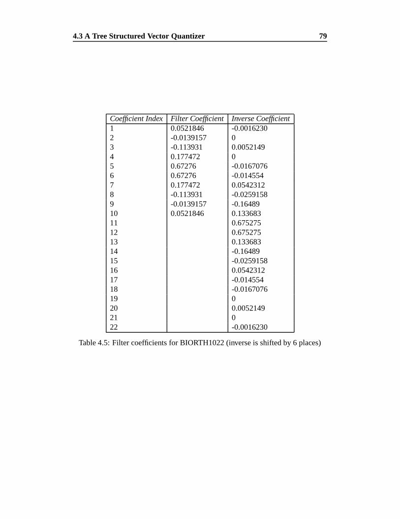
4.3 A Tree Structured Vector Quantizer 79
Coefficient Index Filter Coefficient Inverse Coefficient1 0.0521846 -0.00162302 -0.0139157 03 -0.113931 0.00521494 0.177472 05 0.67276 -0.01670766 0.67276 -0.0145547 0.177472 0.05423128 -0.113931 -0.02591589 -0.0139157 -0.1648910 0.0521846 0.13368311 0.67527512 0.67527513 0.13368314 -0.1648915 -0.025915816 0.054231217 -0.01455418 -0.016707619 020 0.005214921 022 -0.0016230
Table 4.5: Filter coefficients for BIORTH1022 (inverse is shifted by 6 places)
4.3 A Tree Structured Vector Quantizer 80
from. Vector Quantization is a common method of providing lossy data compres-
sion. A conventional vector quantizer works by providing a codebook of vectors
which is used to approximate input vectors. The main problem with general VQ
methods is that they are highly computationally intensive. One method of over-
coming this is to structure the quantizer. A particular example of this subclass is
the tree structured vector quantizer. There have been some attempts to generate
Tree Structured Vector Quantizers [PC94] [BPL95]. These, however, work in an
off-line manner (all the data must be present when the tree is built) or impose
some condition on the source. For the present application, an incremental method
is desirable. Using a tree structured vector quantizer, the pool of previously en-
coded blocks can be structured on-line and searched quickly. This is achieved by
combining a simple on-line tree-growing algorithm with restructuring of the tree,
using a modified form of the Linde-Buzo-Gray (LBG) [LBG80] algorithm.
Consider, therefore, a set of data in the Euclidean k-space,� ��� � � � � ' � � � ' � �
� � � � �. Assuming
� � �, it is possible to partition the data into two clusters, �
and � � , separated by a decision hyperplane, defined by
� � � ��� � � " � � ����
� � � � � ����
� � � � � (4.2)
where � and � � are the centroids of the clusters, as shown in Figure 4.4. The tree
is based on the recursive application of this partitioning.
Expanding the condition in equation 4.2
� ����
� � � � � ����
� � � � (4.3)
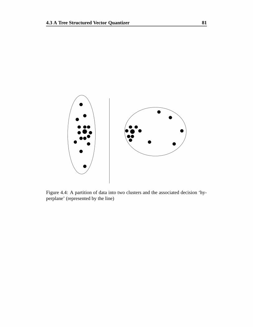
4.3 A Tree Structured Vector Quantizer 81
Figure 4.4: A partition of data into two clusters and the associated decision ‘hy-perplane’ (represented by the line)
4.3 A Tree Structured Vector Quantizer 82
gives us� � � � � � � � � � � � � � � � � � � � (4.4)
Hence, � � � � is the direction of the decision hyperplane normal and � � � � � � � � � is the distance along the normal to the point of intersection with the hyperplane
itself. For ease of notation, define , - � � � � � � � �and / - � � � � � � � � � � � �
at node+
.
Each node,+
, in the tree structured vector quantizer will contain pointers to its
child and parent nodes, the pair � , - ' /0- � defined above, a data vector,� - , a dis-
tortion measure,� - , and the number of nodes in the immediate subtree (the usage
count), ��- . The distortion measure will be used for variable rate coding, and is
an average of the distortions of the child nodes.
Given a new vector, � , it is a simple to decide which cluster the vector should lie
in, without calculating the mean square error between the new vector and each
of the cluster centroids. All that is required is to calculate the value of� � � ,.- .
Obviously,� � � � ,.- � /0- if � � � � � � � ,.- /0- if � � � � (4.5)
with an arbitrary choice being made if equality occurs.
All dichotomies down a particular path are evaluated until a leaf node is reached.
As each node is passed, its average distortion� - is updated by the following
4.3 A Tree Structured Vector Quantizer 83
simple counting argument
� - �� � - � ��- � � � � � ' � - �� - � � (4.6)
follwed by an increment of �#- .
Once a leaf node has been reached, a comparison is made to see if the vector to
be added is already present in the leaf node (or is sufficiently close to the vector
stored in the leaf node). If it is, the usage count of the leaf is incremented and
no more is done. Otherwise, two child nodes are spawned from the old leaf node.
One of these has the data from the old leaf copied down and the other has the new
data placed in it. The average distortion between the old leaf node and the two
new children is then calculated and stored in the old leaf node, followed by the
hyperplane normal direction and intersection point. It is worth noting that if the
old leaf has a usage count greater than one, this is copied down to the duplicate
child node.
In summary, adding a vector to the tree proceeds in the following way.
� If the tree is empty
– Create new root node containing the supplied data. Nothing more is
done.
� If the tree is non-empty
– At each node, evaluate� � � ,.- to decide which path to follow. Update
4.3 A Tree Structured Vector Quantizer 84
the paramaters in each node passed by equation 4.6. Repeat until a
leaf node is reached.
– At the leaf node, check if� ��� ' , - � � �
, for some threshold,�
. If so,
increase the usage count of the node and finish
– If� � � ' ,.- � � �
, create two nodes subordinate to+
. Copy the datum
and other parameters from node+
to the right hand node and place
the new datum in the left hand node.
– Re-calculate the hyperplane parameters for node+
Since the separating hyperplanes are fixed by their placement between the first
two vectors subordinate to a node, it is quite likely that the tree will become un-
balanced. To combat this, a method for restructuring subtrees has been designed,
based on the Linde-Buzo-Gray vector quantizer design algorithm [LBG80].
4.3.1 The Linde-Buzo-Gray Vector Quantizer Design Algorithm
The LBG algorithm for vector quantizer design [LBG80] is used to design near-
optimal block quantizers with a given number of representative vectors. The quan-
tizer is trained by a sequence of training data, usually taken to be representative
of the population that the quantizer must encode. The algorithm produces an op-
timum partition of the training set. This is simply extended into an n-dimensional
optimum partition of Euclidean n-space by the nearest neighbour rule.
Given N, the number of representative vectors in the final quantizer, a training
4.3 A Tree Structured Vector Quantizer 85
sequence� � � � � � � ' � � � ' � � � � ' � � � , and an error threshold � � �
, the
algorithm proceeds as follows
� Initialisation
– Given� � � � , set
�� � � � � � �� where
�� is the centroid of the training
sequence.
– Given�� � � � � , containing M vectors, perturb each vector in the set by
a small, fixed vector, � . So, each � � � �� � � � � is replaced by the two
vectors� �*� � � ' �*�
�
� � � �� � � � � � . Set M=2M.
– Repeat previous step until � � � . Then, the resultant set�� � � � � is
the initial set to which the partitioning algorithm is applied.
� Partitioning
– Given�� � , find the minimum distortion partition
� � �� � � � � � � � � �
� ' � � � ' � � of the training set by assigning each vector � � to a cluster
� � using the rule
� � � � � � � � � � �*� � � � � � � � � � � � (4.7)
– Calculate the average distortion
� � ��
�" ���� � � � � � ��� � � � � ' � � � (4.8)
If ���� � �
�
�� � � stop with
�� � as the final set of representative vectors.
4.3 A Tree Structured Vector Quantizer 86
– Re-estimate the centroids of the clusters� � � � . Set
�� � � � � �� � � � �
� ' � � � ' � � . Set � � � � �. Repeat the partitioning step.
4.3.2 Restructuring an Unbalanced Tree
Before a restructure is performed, it must first be decided where (or if) the tree
is actually unbalanced. Since the usage count in any node represents the number
of leaf data nodes below it, a comparison of usage counts of sibling nodes is an
appropriate measure of how unbalanced the subtree is. Note that the root node
usage count is the total number of leaf node data vectors in the subtree.
A recursive traversal down the tree is performed from the root. At any point,
� ������� ' � ��� � � ' � � ��� � , the usage counts in the subtree root node and the current left
and right child nodes are known and it is simple to calculate� � and
��
�� � � �
�� � �������� ��� � � � (4.9)
� � � �� ��� � � ������ � ��� � � (4.10)
(4.11)
and so� � � � � � � �
�� � ��� � �� � ��� � � � (4.12)
A subtree is deemed unbalanced if � � � � � � � � � � . Once an unbalanced subtree
is found, the leaf data are extracted and the subtree is deleted. The subtree root
data value is set to the centroid of all the leaf data. Then, the LBG algorithm is
4.3 A Tree Structured Vector Quantizer 87
run on the leaf data to produce two cluster centroids. These centroids are used as
the data for the child nodes of the subtree root node. The separating hyperplane
is calculated and its normal vector and intersection point are stored in the subtree
root. The application of the LBG algorithm implicitly generates two new subtree
root nodes and two sets of leaf data nodes. These are the two sets of data that
constitute the clusters generated by the algorithm. The procedure is applied recur-
sively until only two data vectors remain. Then, a simple split is performed and
the subtree is fully restructured. The final procedure in the restructure is to work
back up the subtree to the subtree root in order to update the usage counts in each
node. This is a simple by-product of the recursive nature of the procedure.
4.3.3 Variable rate coding using the TSVQ
The tree structured vector quantizer can be used to perform variable rate coding.
The rate can be varied by either constraining the maximum number of bits used to
encode a given vector or by a maximum mean square error per vector. Since each
node contains both a representative vector and the average distortion between the
vector in the current node and its children, a simple comparison will determine if
either the mean square error distortion or the bit rate constraint has been reached.
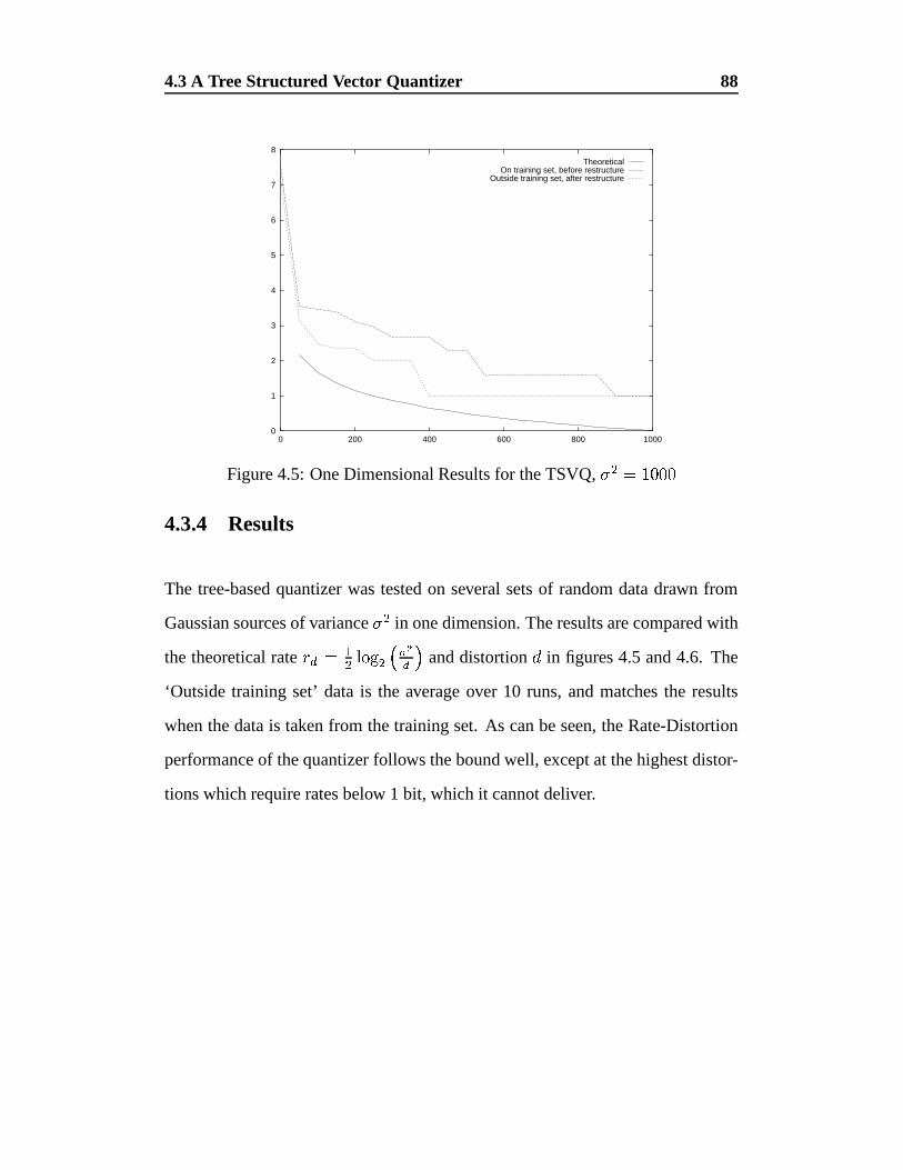
4.3 A Tree Structured Vector Quantizer 88
0
1
2
3
4
5
6
7
8
0 200 400 600 800 1000
TheoreticalOn training set, before restructure
Outside training set, after restructure
Figure 4.5: One Dimensional Results for the TSVQ, � � ��������
4.3.4 Results
The tree-based quantizer was tested on several sets of random data drawn from
Gaussian sources of variance ��� in one dimension. The results are compared with
the theoretical rate� � �
��� ����� � and distortion
�in figures 4.5 and 4.6. The
‘Outside training set’ data is the average over 10 runs, and matches the results
when the data is taken from the training set. As can be seen, the Rate-Distortion
performance of the quantizer follows the bound well, except at the highest distor-
tions which require rates below 1 bit, which it cannot deliver.

4.4 An Oriented Wavelet Image Coding Algorithm 89
0
1
2
3
4
5
6
7
8
0 50 100 150 200
TheoreticalOn training set, before restructure
Outside training set, after restructure
Figure 4.6: One Dimensional Results for the TSVQ, � � �� ���
4.4 An Oriented Wavelet Image Coding Algorithm
The oriented wavelet subband decomposition presented previously refines the ori-
entation selectivity of the wavelet transform without increasing the volume of data
produced. The tree structured vector quantizer gives a method of finding nearest-
neighbour matches in logarithmic time. The two schemes appear to complement
each other well and form the basis of a compression scheme which should be more
efficient than that of the previous chapter.
4.4 An Oriented Wavelet Image Coding Algorithm 90
4.4.1 Algorithm Overview
The algorithm for the oriented wavelet subband coder is broadly similar to that of
the predictive wavelet coder presented in Chapter 3. Figure 4.7 gives an algorithm
description of the modified coder. Given the number of levels to decompose the
image, � , and the level to predict from, � , the real wavelet transform is applied to
decompose the image to � levels. The lowpass and the � ��
� � lowest frequency
highpass levels of the wavelet tree are then linearly quantized and encoded as in
the original algorithm. The quantizer and arithmetic coder are again controlled by
a rate parameter that specifies the quantizer bin size and the number of symbols
that the arithmetic coder can encode. The oriented wavelet transform is then ap-
plied to the quantized real wavelet data. The encoding process proceeds from one
level to the next. It requires two wavelet coefficient levels, one to predict from and
one to approximate. Given these levels, the algorithm begins by scanning the six
complex-valued wavelet coefficient bands and extracting (possibly overlapping)
blocks of data on a�
-pixel grid. Any block whose energy is below a threshold
is treated as noise and ignored. The coder implements two tree structured vec-
tor quantizers, detailed earlier in this chapter. One is used for the horizontal and
vertical derived complex bands and one for the diagonal derived complex bands.
As suggested in section 4.1, the horizontal and vertical derived subbands are suf-
ficiently related to allow one vector quantization tree to be used for them. The
diagonal bands are not related to the others in any simple way and so are treated
separately. The extracted blocks are added to the relevant tree structured vector
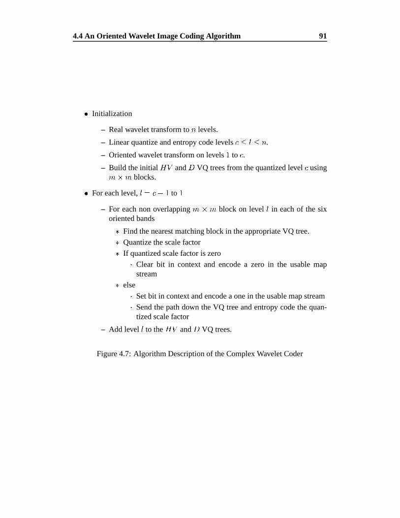
4.4 An Oriented Wavelet Image Coding Algorithm 91
� Initialization
– Real wavelet transform to � levels.
– Linear quantize and entropy code levels � � � � � .
– Oriented wavelet transform on levels�
to � .– Build the initial
� !and � VQ trees from the quantized level � using� � � blocks.
� For each level,� � �
�
�to�
– For each non overlapping � � � block on level�
in each of the sixoriented bands
� Find the nearest matching block in the appropriate VQ tree.� Quantize the scale factor� If quantized scale factor is zero
� Clear bit in context and encode a zero in the usable mapstream
� else� Set bit in context and encode a one in the usable map stream� Send the path down the VQ tree and entropy code the quan-
tized scale factor
– Add level�
to the� !
and � VQ trees.
Figure 4.7: Algorithm Description of the Complex Wavelet Coder
4.4 An Oriented Wavelet Image Coding Algorithm 92
quantizer, after being transformed into a canonical orientation (relative to the ap-
propriate tree) and normalized. The canonical orientations are taken, arbitrarily,
as the orientation of band 1 for the HV tree and that of band 3 for the D tree.
Since the tree structured vector quantizers are populated from data known to both
the encoder and decoder, explicit transmission of the codebooks is avoided. The
encoding process for a given level is simple. The six complex sub-bands are par-
titioned into non-overlapping blocks,as in figure 4.8. The shaded bands are not
coded and will be reconstructed using the hermitian symmetry property of the
transform. The blocks from the same relative position in each of the six bands
are encoded in turn. That is, for each band, block number�
is encoded, followed
by block number�
and so on. The blocks are transformed into the canonical ori-
entation of the appropriate vector quantizer tree and the tree is searched for the
best matching vector. The search can be terminated by a maximum path length
constraint, a minimum error constraint or by finding a leaf node. The constraints
on maximum path length and minimum error are configuration parameters of the
encoder. A simple inner product between the source vector and the vector found
in the tree yields the scale factor. Associated with each block position is a six bit
context value. The context consists of ‘code/not code’ decisions for each oriented
wavelet subband. The ‘code/not code’ decision is based solely on the quantized
scale factor: if the quantized scale factor is not zero, the appropriate bit is set in
the context map and a one flag is sent to the decoder, indicating that parameters
are present for this prediction. If the scale factor quantizes to zero, the appropriate
bit in the context map is cleared and a zero flag is sent to the decoder. If the block
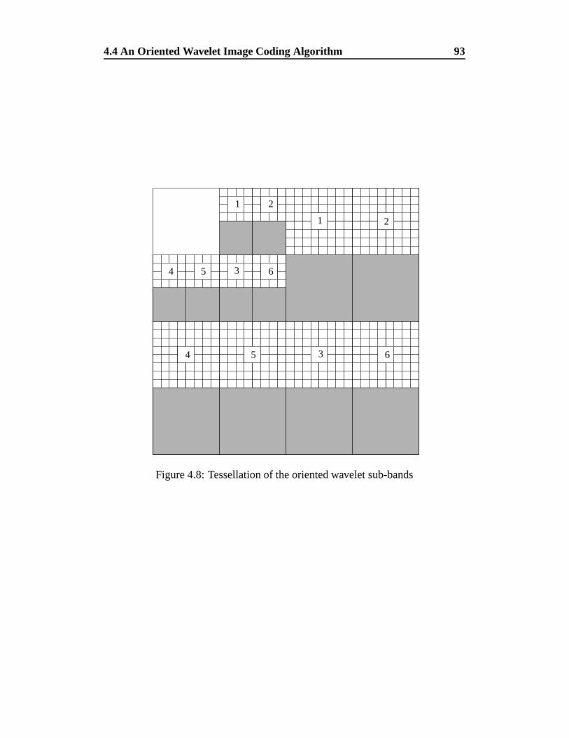
4.4 An Oriented Wavelet Image Coding Algorithm 93
1 2
3 64 5
1
3 654
2
Figure 4.8: Tessellation of the oriented wavelet sub-bands
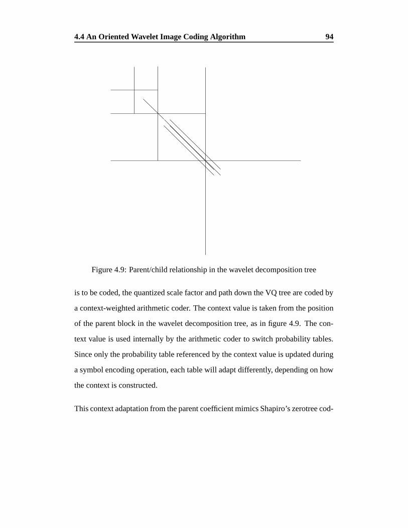
4.4 An Oriented Wavelet Image Coding Algorithm 94
Figure 4.9: Parent/child relationship in the wavelet decomposition tree
is to be coded, the quantized scale factor and path down the VQ tree are coded by
a context-weighted arithmetic coder. The context value is taken from the position
of the parent block in the wavelet decomposition tree, as in figure 4.9. The con-
text value is used internally by the arithmetic coder to switch probability tables.
Since only the probability table referenced by the context value is updated during
a symbol encoding operation, each table will adapt differently, depending on how
the context is constructed.
This context adaptation from the parent coefficient mimics Shapiro’s zerotree cod-
4.4 An Oriented Wavelet Image Coding Algorithm 95
ing [Sha93]. For example, if the component coefficients are not coded at a position
on level � , the child coefficients at level � � � are unlikely to be coded. Thus, the
probability distribution for the generated context will be heavily skewed towards
zero, for both the scale factor and usable map coders. The relation to Shapiro’s ze-
rotree structure is obvious. Shapiro also postulates that if a coefficient at a given
scale is zero, it is probable that all its descendant coefficients will also be zero.
He encodes this decision with an explicit symbol to indicate an insignificant co-
efficient tree root. The coder presented here, using the context adaptation, will
implicitly adapt to this situation and send little or no information for the insignif-
icant coefficient tree.
4.4.2 The Coder Context
Visual representations of the coder context are shown in figure 4.10 for both high
and low bit rates, resulting from coding the Lena image. In the figures, which
have been resized for ease of interpretation, a black pixel indicates that the block
originating at that point was coded in at least one of the sub-bands, and white
indicates that the block was ignored. Figures 4.10(a) and (b) show the context
that results from encoding level 2 in the Lena image using fine ( � � � � ' �
' � � ��� ����� ' � � ��� � ) and coarse ( � � ��� ' �
��� ' � � � � ��� � � ' � � � ��� � ) quantiz-
ers. Figures 4.10(c) and (d) show similar results for level 1. At the high bit rates,
more information is expended coding the higher frequency areas of the image,
like the hair and feathers. At lower bit rates, it is obvious that these areas are
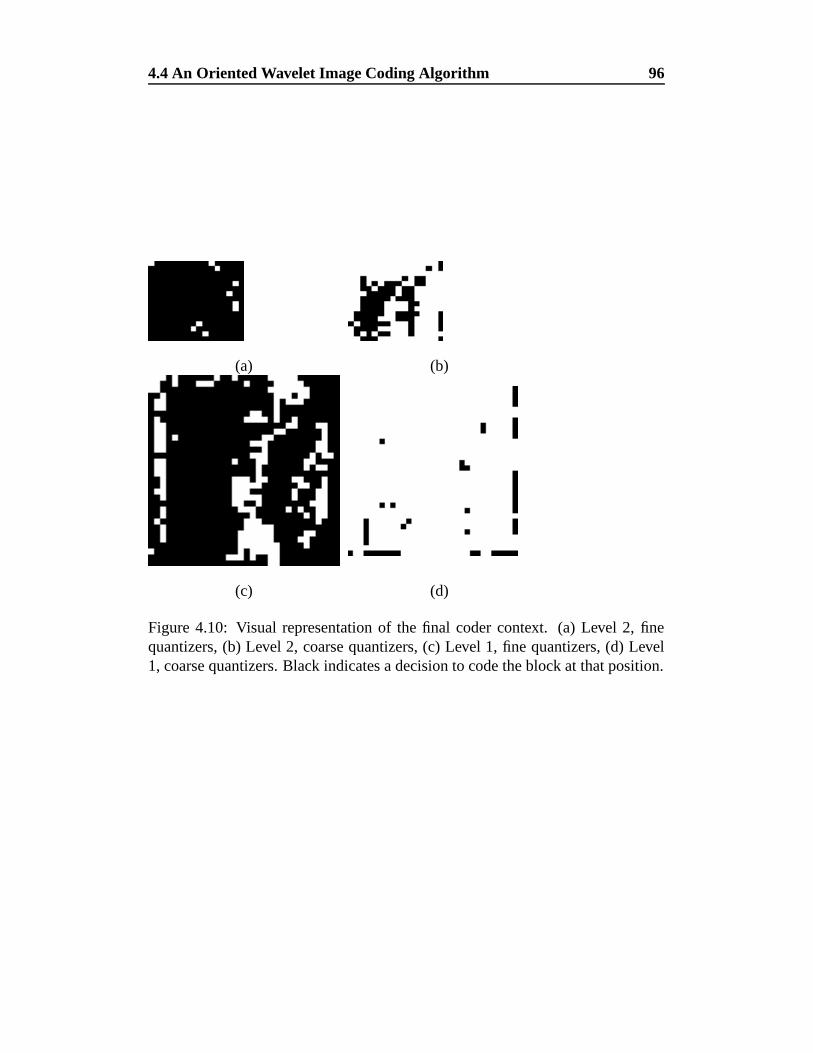
4.4 An Oriented Wavelet Image Coding Algorithm 96
(a) (b)
(c) (d)
Figure 4.10: Visual representation of the final coder context. (a) Level 2, finequantizers, (b) Level 2, coarse quantizers, (c) Level 1, fine quantizers, (d) Level1, coarse quantizers. Black indicates a decision to code the block at that position.

4.4 An Oriented Wavelet Image Coding Algorithm 97
forgone for the more dominant features. Also, the quadtree/zerotree type struc-
ture is demonstrated by these diagrams. If a block is not coded on level 2, it is
rarely coded on level 1. The adaptive context used by this system appears to emu-
late Shapiro’s zerotree structure reasonably well and also agrees with the intuitive
idea of scale invariance of edge features [ZM90].
4.4.3 Rate Control
The oriented wavelet coder can be rate-controlled in a number of independent
ways. The simplest and most obvious method for rate control is to alter the lin-
ear quantizer bin size that is used to quantize the multiplicative scale factors of the
vector quantizer entries. This is the rate control method used in most of the results
presented here. Furthermore, since the vector quantizer is tree structured, it can
perform variable rate coding, as in section 4.3.3. It can code to a specified bit rate
by limiting the tree traversal, effectively altering the vector quantizer codebook
size, or to a specified error by using the average distortion value contained in each
node. The quantizer used to scalar quantize the lower frequency wavelet coeffi-
cients can also be varied as can the dimensionality of the vectors. The combined
parameter space for the coder is far too large to explore fully, but a number of tests
have been performed to identify useful values.
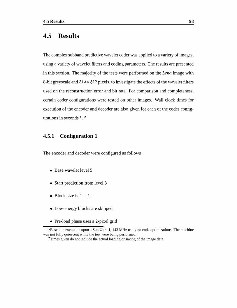
4.5 Results 98
4.5 Results
The complex subband predictive wavelet coder was applied to a variety of images,
using a variety of wavelet filters and coding parameters. The results are presented
in this section. The majority of the tests were performed on the Lena image with
8-bit greyscale and����� � �����
pixels, to investigate the effects of the wavelet filters
used on the reconstruction error and bit rate. For comparison and completeness,
certain coder configurations were tested on other images. Wall clock times for
execution of the encoder and decoder are also given for each of the coder config-
urations in seconds. �
4.5.1 Configuration 1
The encoder and decoder were configured as follows
� Base wavelet level 5
� Start prediction from level 3
� Block size is� � �
� Low-energy blocks are skipped
� Pre-load phase uses a 2-pixel grid�Based on execution upon a Sun Ultra 1, 143 MHz using no code optimizations. The machine
was not fully quiescent while the test were being performed.�Times given do not include the actual loading or saving of the image data.
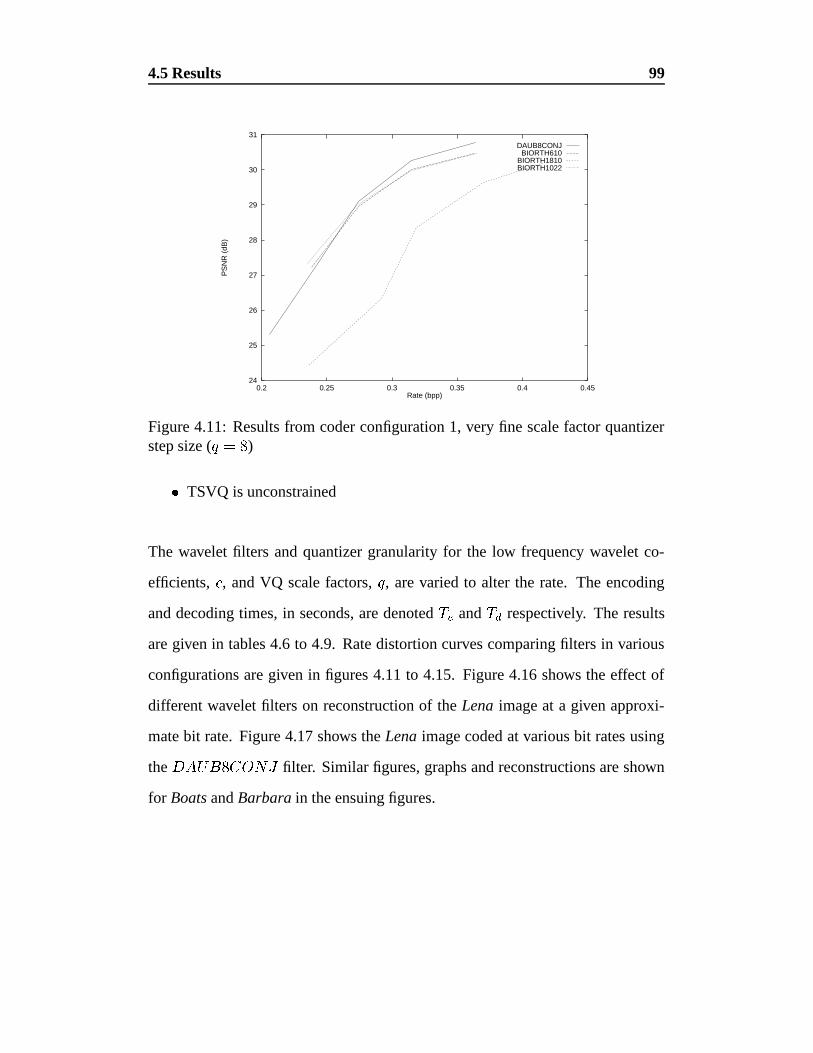
4.5 Results 99
24
25
26
27
28
29
30
31
0.2 0.25 0.3 0.35 0.4 0.45
PS
NR
(dB
)
Rate (bpp)
DAUB8CONJBIORTH610
BIORTH1810BIORTH1022
Figure 4.11: Results from coder configuration 1, very fine scale factor quantizerstep size ( � )
� TSVQ is unconstrained
The wavelet filters and quantizer granularity for the low frequency wavelet co-
efficients, � , and VQ scale factors, , are varied to alter the rate. The encoding
and decoding times, in seconds, are denoted�� and
� � respectively. The results
are given in tables 4.6 to 4.9. Rate distortion curves comparing filters in various
configurations are given in figures 4.11 to 4.15. Figure 4.16 shows the effect of
different wavelet filters on reconstruction of the Lena image at a given approxi-
mate bit rate. Figure 4.17 shows the Lena image coded at various bit rates using
the ����� � � � filter. Similar figures, graphs and reconstructions are shown
for Boats and Barbara in the ensuing figures.
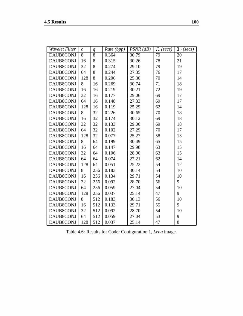
4.5 Results 100
Wavelet Filter c q Rate (bpp) PSNR (dB)�� (secs)
� � (secs)DAUB8CONJ 8 8 0.364 30.79 79 20DAUB8CONJ 16 8 0.315 30.26 78 21DAUB8CONJ 32 8 0.274 29.10 79 19DAUB8CONJ 64 8 0.244 27.35 76 17DAUB8CONJ 128 8 0.206 25.30 70 14DAUB8CONJ 8 16 0.269 30.74 71 18DAUB8CONJ 16 16 0.219 30.21 72 19DAUB8CONJ 32 16 0.177 29.06 69 17DAUB8CONJ 64 16 0.148 27.33 69 17DAUB8CONJ 128 16 0.119 25.29 62 14DAUB8CONJ 8 32 0.226 30.65 70 18DAUB8CONJ 16 32 0.174 30.12 69 18DAUB8CONJ 32 32 0.133 29.00 69 18DAUB8CONJ 64 32 0.102 27.29 70 17DAUB8CONJ 128 32 0.077 25.27 58 13DAUB8CONJ 8 64 0.199 30.49 65 15DAUB8CONJ 16 64 0.147 29.98 63 15DAUB8CONJ 32 64 0.106 28.90 63 15DAUB8CONJ 64 64 0.074 27.21 62 14DAUB8CONJ 128 64 0.051 25.22 54 12DAUB8CONJ 8 256 0.183 30.14 54 10DAUB8CONJ 16 256 0.134 29.71 54 10DAUB8CONJ 32 256 0.092 28.70 56 9DAUB8CONJ 64 256 0.059 27.04 54 10DAUB8CONJ 128 256 0.037 25.14 47 9DAUB8CONJ 8 512 0.183 30.13 56 10DAUB8CONJ 16 512 0.133 29.71 55 9DAUB8CONJ 32 512 0.092 28.70 54 10DAUB8CONJ 64 512 0.059 27.04 53 9DAUB8CONJ 128 512 0.037 25.14 47 8
Table 4.6: Results for Coder Configuration 1, Lena image.
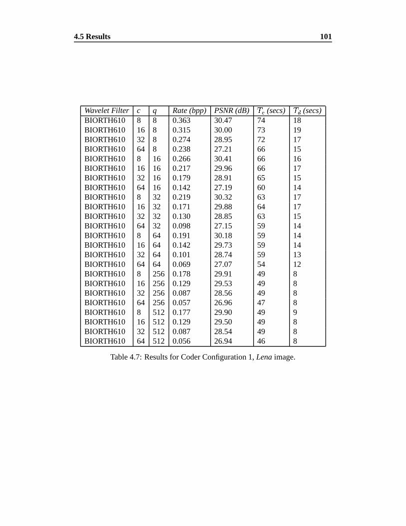
4.5 Results 101
Wavelet Filter c q Rate (bpp) PSNR (dB)�� (secs)
� � (secs)BIORTH610 8 8 0.363 30.47 74 18BIORTH610 16 8 0.315 30.00 73 19BIORTH610 32 8 0.274 28.95 72 17BIORTH610 64 8 0.238 27.21 66 15BIORTH610 8 16 0.266 30.41 66 16BIORTH610 16 16 0.217 29.96 66 17BIORTH610 32 16 0.179 28.91 65 15BIORTH610 64 16 0.142 27.19 60 14BIORTH610 8 32 0.219 30.32 63 17BIORTH610 16 32 0.171 29.88 64 17BIORTH610 32 32 0.130 28.85 63 15BIORTH610 64 32 0.098 27.15 59 14BIORTH610 8 64 0.191 30.18 59 14BIORTH610 16 64 0.142 29.73 59 14BIORTH610 32 64 0.101 28.74 59 13BIORTH610 64 64 0.069 27.07 54 12BIORTH610 8 256 0.178 29.91 49 8BIORTH610 16 256 0.129 29.53 49 8BIORTH610 32 256 0.087 28.56 49 8BIORTH610 64 256 0.057 26.96 47 8BIORTH610 8 512 0.177 29.90 49 9BIORTH610 16 512 0.129 29.50 49 8BIORTH610 32 512 0.087 28.54 49 8BIORTH610 64 512 0.056 26.94 46 8
Table 4.7: Results for Coder Configuration 1, Lena image.
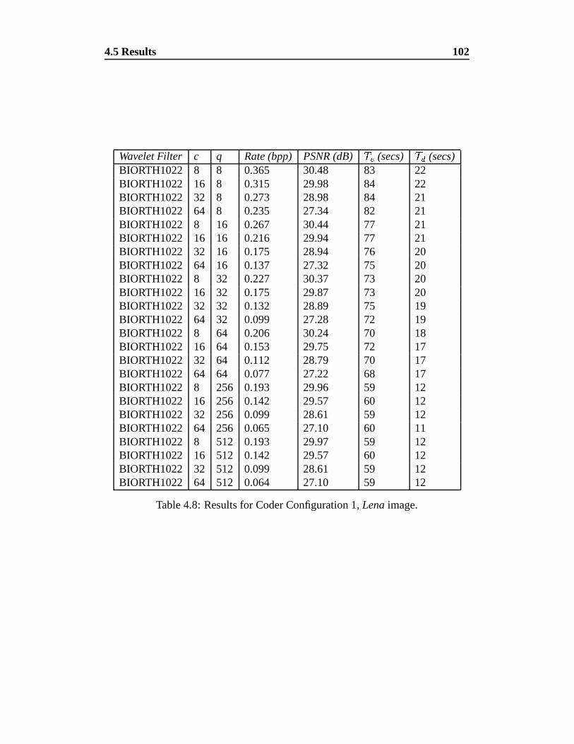
4.5 Results 102
Wavelet Filter c q Rate (bpp) PSNR (dB)�� (secs)
� � (secs)BIORTH1022 8 8 0.365 30.48 83 22BIORTH1022 16 8 0.315 29.98 84 22BIORTH1022 32 8 0.273 28.98 84 21BIORTH1022 64 8 0.235 27.34 82 21BIORTH1022 8 16 0.267 30.44 77 21BIORTH1022 16 16 0.216 29.94 77 21BIORTH1022 32 16 0.175 28.94 76 20BIORTH1022 64 16 0.137 27.32 75 20BIORTH1022 8 32 0.227 30.37 73 20BIORTH1022 16 32 0.175 29.87 73 20BIORTH1022 32 32 0.132 28.89 75 19BIORTH1022 64 32 0.099 27.28 72 19BIORTH1022 8 64 0.206 30.24 70 18BIORTH1022 16 64 0.153 29.75 72 17BIORTH1022 32 64 0.112 28.79 70 17BIORTH1022 64 64 0.077 27.22 68 17BIORTH1022 8 256 0.193 29.96 59 12BIORTH1022 16 256 0.142 29.57 60 12BIORTH1022 32 256 0.099 28.61 59 12BIORTH1022 64 256 0.065 27.10 60 11BIORTH1022 8 512 0.193 29.97 59 12BIORTH1022 16 512 0.142 29.57 60 12BIORTH1022 32 512 0.099 28.61 59 12BIORTH1022 64 512 0.064 27.10 59 12
Table 4.8: Results for Coder Configuration 1, Lena image.
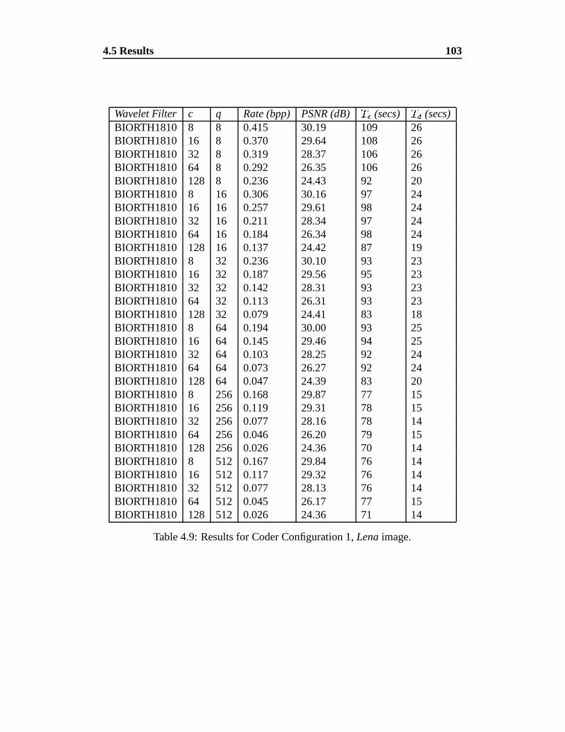
4.5 Results 103
Wavelet Filter c q Rate (bpp) PSNR (dB)�� (secs)
� � (secs)BIORTH1810 8 8 0.415 30.19 109 26BIORTH1810 16 8 0.370 29.64 108 26BIORTH1810 32 8 0.319 28.37 106 26BIORTH1810 64 8 0.292 26.35 106 26BIORTH1810 128 8 0.236 24.43 92 20BIORTH1810 8 16 0.306 30.16 97 24BIORTH1810 16 16 0.257 29.61 98 24BIORTH1810 32 16 0.211 28.34 97 24BIORTH1810 64 16 0.184 26.34 98 24BIORTH1810 128 16 0.137 24.42 87 19BIORTH1810 8 32 0.236 30.10 93 23BIORTH1810 16 32 0.187 29.56 95 23BIORTH1810 32 32 0.142 28.31 93 23BIORTH1810 64 32 0.113 26.31 93 23BIORTH1810 128 32 0.079 24.41 83 18BIORTH1810 8 64 0.194 30.00 93 25BIORTH1810 16 64 0.145 29.46 94 25BIORTH1810 32 64 0.103 28.25 92 24BIORTH1810 64 64 0.073 26.27 92 24BIORTH1810 128 64 0.047 24.39 83 20BIORTH1810 8 256 0.168 29.87 77 15BIORTH1810 16 256 0.119 29.31 78 15BIORTH1810 32 256 0.077 28.16 78 14BIORTH1810 64 256 0.046 26.20 79 15BIORTH1810 128 256 0.026 24.36 70 14BIORTH1810 8 512 0.167 29.84 76 14BIORTH1810 16 512 0.117 29.32 76 14BIORTH1810 32 512 0.077 28.13 76 14BIORTH1810 64 512 0.045 26.17 77 15BIORTH1810 128 512 0.026 24.36 71 14
Table 4.9: Results for Coder Configuration 1, Lena image.
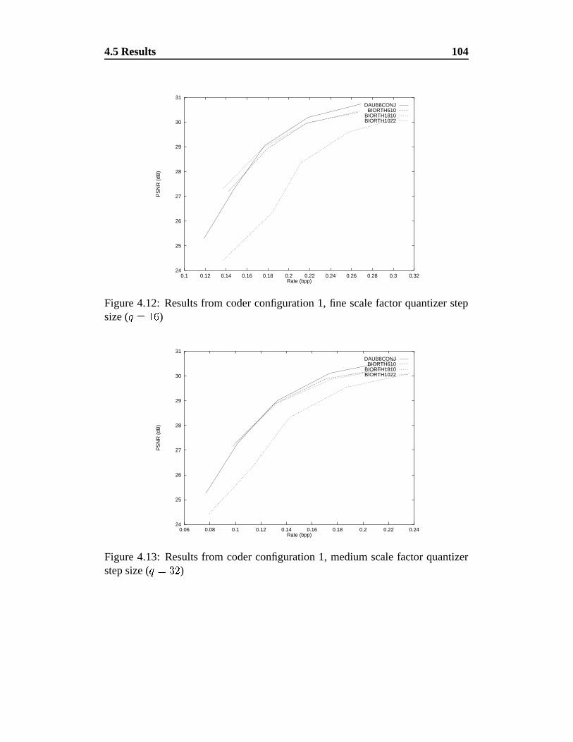
4.5 Results 104
24
25
26
27
28
29
30
31
0.1 0.12 0.14 0.16 0.18 0.2 0.22 0.24 0.26 0.28 0.3 0.32
PS
NR
(dB
)
Rate (bpp)
DAUB8CONJBIORTH610
BIORTH1810BIORTH1022
Figure 4.12: Results from coder configuration 1, fine scale factor quantizer stepsize ( �
� �)
24
25
26
27
28
29
30
31
0.06 0.08 0.1 0.12 0.14 0.16 0.18 0.2 0.22 0.24
PS
NR
(dB
)
Rate (bpp)
DAUB8CONJBIORTH610
BIORTH1810BIORTH1022
Figure 4.13: Results from coder configuration 1, medium scale factor quantizerstep size ( �
�)
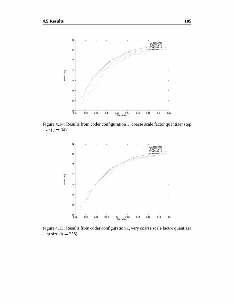
4.5 Results 105
24
25
26
27
28
29
30
31
0.04 0.06 0.08 0.1 0.12 0.14 0.16 0.18 0.2 0.22
PS
NR
(dB
)
Rate (bpp)
DAUB8CONJBIORTH610
BIORTH1810BIORTH1022
Figure 4.14: Results from coder configuration 1, coarse scale factor quantizer stepsize ( �
� �)
24
25
26
27
28
29
30
31
0.02 0.04 0.06 0.08 0.1 0.12 0.14 0.16 0.18 0.2
PS
NR
(dB
)
Rate (bpp)
DAUB8CONJBIORTH610
BIORTH1810BIORTH1022
Figure 4.15: Results from coder configuration 1, very coarse scale factor quantizerstep size ( �
� ���)

4.5 Results 106
(a)
(b)
Figure 4.16: Reconstructions from coder configuration 1 Lena image showing ef-fect of filter on quality; medium scale factor quantizer step size ( � � � '
�� �), approx
� � ��������� (a) DAUB8CONJ,� � � � � ' � � ����������� , (b) BIORTH610,
� � � � � ' � � ��� � �����

4.5 Results 107
(c)
(d)
Figure 4.16: Reconstructions from coder configuration 1 Lena image showing ef-fect of filter on quality; medium scale factor quantizer step size ( � � � '
�� �), approx
� � ��������� (c) BIORTH1810,� � � � � ' � � ��� � � � , (d) BIORTH1022,
� � � � � ' � � � ��� �����
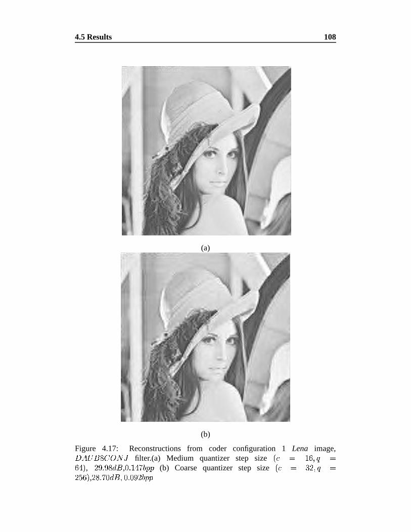
4.5 Results 108
(a)
(b)
Figure 4.17: Reconstructions from coder configuration 1 Lena image,� ��� �� ���� filter.(a) Medium quantizer step size � � � � � '
�� � � , � � � � � ,
� � � � � ����� (b) Coarse quantizer step size � � � � ' �
� ��� � , � � � � � ' � � � � � � � �
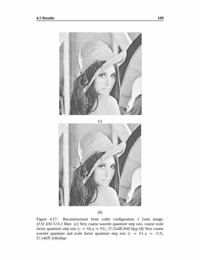
4.5 Results 109
(c)
(d)
Figure 4.17: Reconstructions from coder configuration 1 Lena image,� ��� �� ���� filter. (c) Very coarse wavelet quantizer step size, coarse scalefactor quantizer step size � � � ��� '
���� � , � � � ��� � ' � � � � � ����� (d) Very coarse
wavelet quantizer and scale factor quantizer step size � � � ��� ' � ����� � ,
� � � � � � ' � � � � � �����

4.5 Results 110
Wavelet Filter c q Rate (bpp) PSNR (dB)�� (secs)
� � (secs)DAUB8CONJ 8 8 0.399 27.92 85 20DAUB8CONJ 16 8 0.341 27.62 80 19DAUB8CONJ 32 8 0.293 26.79 79 20DAUB8CONJ 64 8 0.259 25.28 79 19DAUB8CONJ 8 16 0.327 27.89 76 19DAUB8CONJ 16 16 0.274 27.59 75 18DAUB8CONJ 32 16 0.222 26.77 78 18DAUB8CONJ 64 16 0.188 25.26 73 21DAUB8CONJ 8 32 0.269 27.82 83 22DAUB8CONJ 16 32 0.215 27.53 74 18DAUB8CONJ 32 32 0.166 26.72 71 19DAUB8CONJ 64 32 0.129 25.22 84 19DAUB8CONJ 8 64 0.230 27.68 78 18DAUB8CONJ 16 64 0.175 27.39 71 18DAUB8CONJ 32 64 0.127 26.60 67 17DAUB8CONJ 64 64 0.090 25.15 82 17DAUB8CONJ 8 256 0.201 27.33 65 9DAUB8CONJ 16 256 0.147 27.05 55 10DAUB8CONJ 32 256 0.100 26.35 54 9DAUB8CONJ 64 256 0.063 24.98 53 9DAUB8CONJ 8 512 0.200 27.31 56 10DAUB8CONJ 16 512 0.147 27.04 83 14DAUB8CONJ 32 512 0.099 26.34 54 10DAUB8CONJ 64 512 0.062 24.97 52 9
Table 4.10: Results for Coder Configuration 1, Boats image
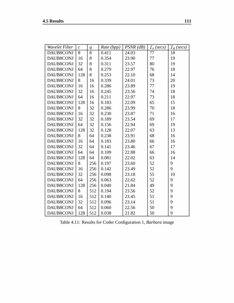
4.5 Results 111
Wavelet Filter c q Rate (bpp) PSNR (dB)�� (secs)
� � (secs)DAUB8CONJ 8 8 0.411 24.03 77 18DAUB8CONJ 16 8 0.354 23.90 77 19DAUB8CONJ 32 8 0.311 23.57 80 19DAUB8CONJ 64 8 0.279 22.97 76 18DAUB8CONJ 128 8 0.253 22.10 68 14DAUB8CONJ 8 16 0.339 24.01 73 20DAUB8CONJ 16 16 0.286 23.89 77 19DAUB8CONJ 32 16 0.245 23.56 74 18DAUB8CONJ 64 16 0.211 22.97 73 18DAUB8CONJ 128 16 0.183 22.09 65 15DAUB8CONJ 8 32 0.286 23.99 70 18DAUB8CONJ 16 32 0.230 23.87 71 16DAUB8CONJ 32 32 0.189 23.54 69 17DAUB8CONJ 64 32 0.156 22.94 69 19DAUB8CONJ 128 32 0.128 22.07 63 13DAUB8CONJ 8 64 0.238 23.91 68 16DAUB8CONJ 16 64 0.183 23.80 66 16DAUB8CONJ 32 64 0.141 23.46 67 17DAUB8CONJ 64 64 0.109 22.88 66 16DAUB8CONJ 128 64 0.081 22.02 63 14DAUB8CONJ 8 256 0.197 23.60 52 9DAUB8CONJ 16 256 0.142 23.49 52 9DAUB8CONJ 32 256 0.098 23.18 55 10DAUB8CONJ 64 256 0.063 22.62 52 9DAUB8CONJ 128 256 0.040 21.84 49 9DAUB8CONJ 8 512 0.194 23.56 52 9DAUB8CONJ 16 512 0.140 23.45 51 9DAUB8CONJ 32 512 0.096 23.14 51 9DAUB8CONJ 64 512 0.060 22.56 50 9DAUB8CONJ 128 512 0.038 21.82 50 9
Table 4.11: Results for Coder Configuration 1, Barbara image
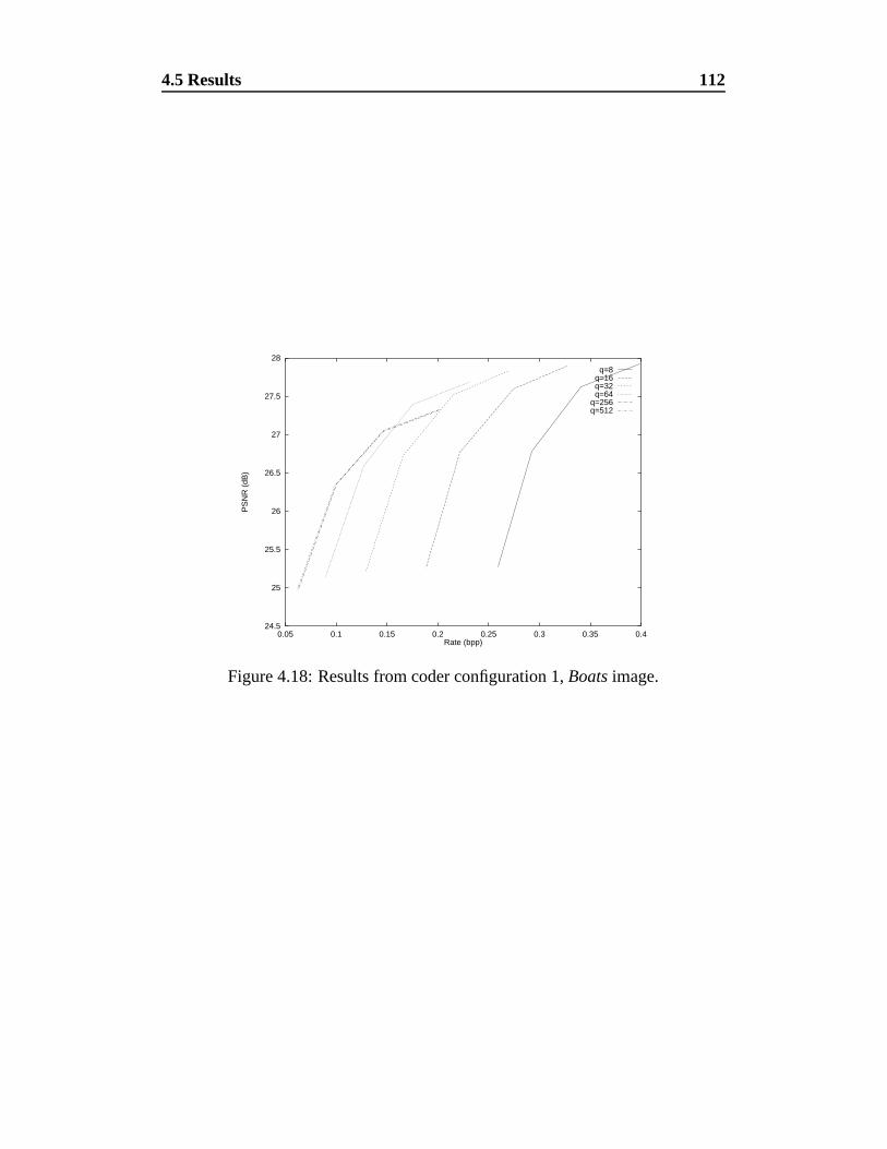
4.5 Results 112
24.5
25
25.5
26
26.5
27
27.5
28
0.05 0.1 0.15 0.2 0.25 0.3 0.35 0.4
PS
NR
(dB
)
Rate (bpp)
q=8q=16q=32q=64
q=256q=512
Figure 4.18: Results from coder configuration 1, Boats image.
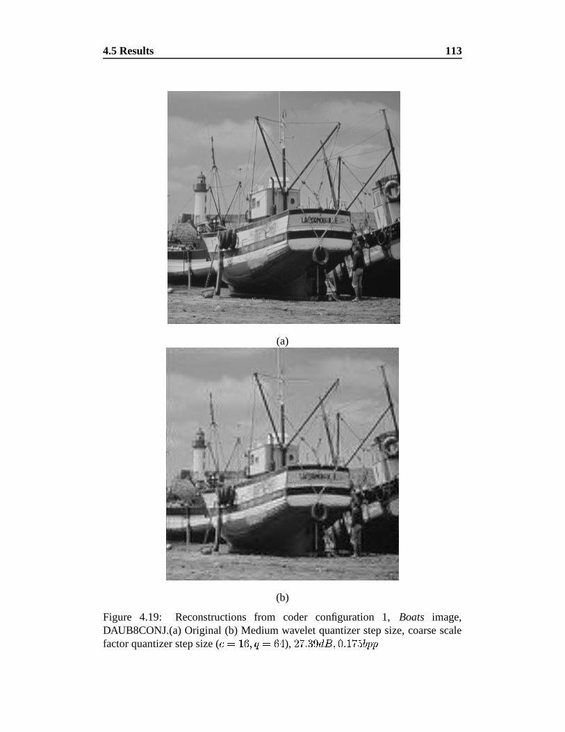
4.5 Results 113
(a)
(b)
Figure 4.19: Reconstructions from coder configuration 1, Boats image,DAUB8CONJ.(a) Original (b) Medium wavelet quantizer step size, coarse scalefactor quantizer step size ( � � ��� '
����
),� � � � � ' � � � � � �����
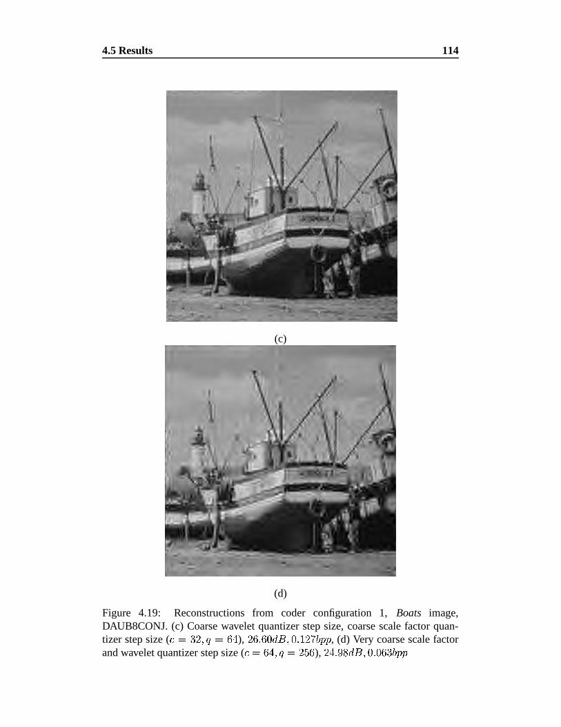
4.5 Results 114
(c)
(d)
Figure 4.19: Reconstructions from coder configuration 1, Boats image,DAUB8CONJ. (c) Coarse wavelet quantizer step size, coarse scale factor quan-tizer step size ( � � � '
����
),��� � ��� � ' � � � � � ����� , (d) Very coarse scale factor
and wavelet quantizer step size ( � � ��� ' �
� � �),� � � � � ' � � ��� �����
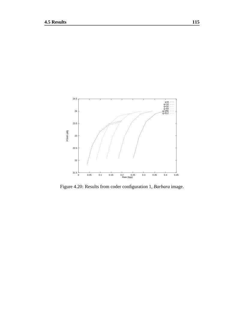
4.5 Results 115
21.5
22
22.5
23
23.5
24
24.5
0 0.05 0.1 0.15 0.2 0.25 0.3 0.35 0.4 0.45
PS
NR
(dB
)
Rate (bpp)
q=8q=16q=32q=64
q=256q=512
Figure 4.20: Results from coder configuration 1, Barbara image.
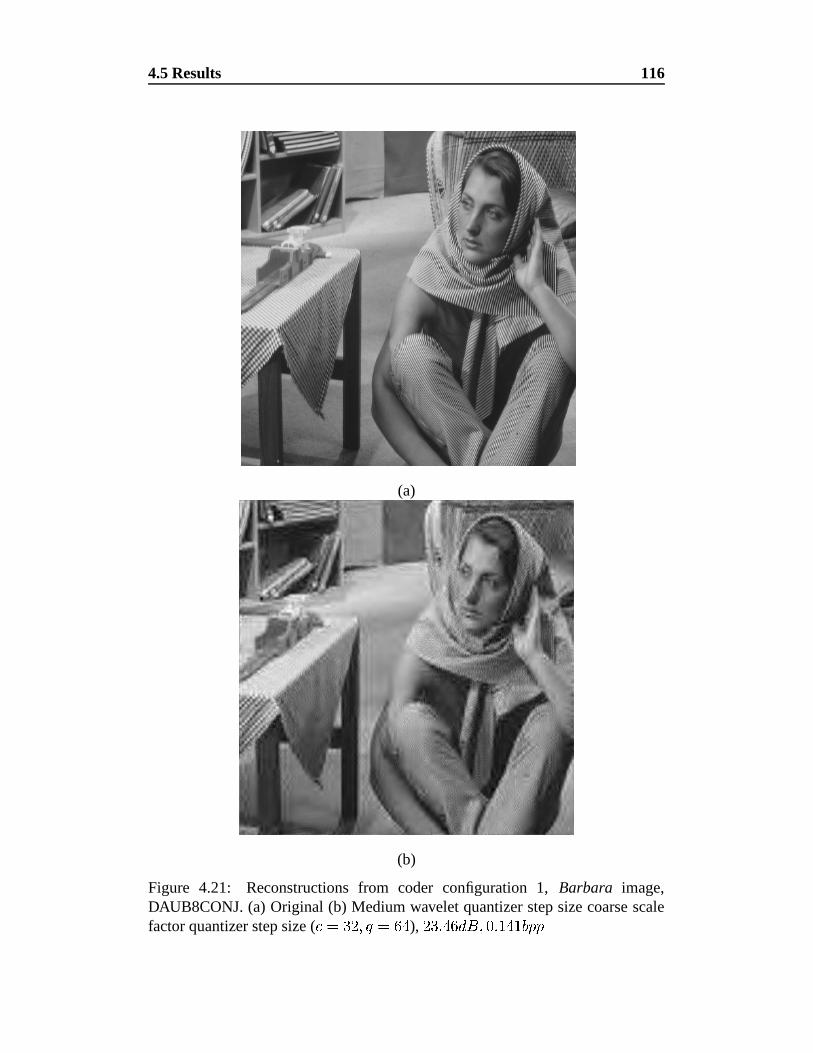
4.5 Results 116
(a)
(b)
Figure 4.21: Reconstructions from coder configuration 1, Barbara image,DAUB8CONJ. (a) Original (b) Medium wavelet quantizer step size coarse scalefactor quantizer step size ( � �� � '
����
),� � ��� � ' � � � � � �����
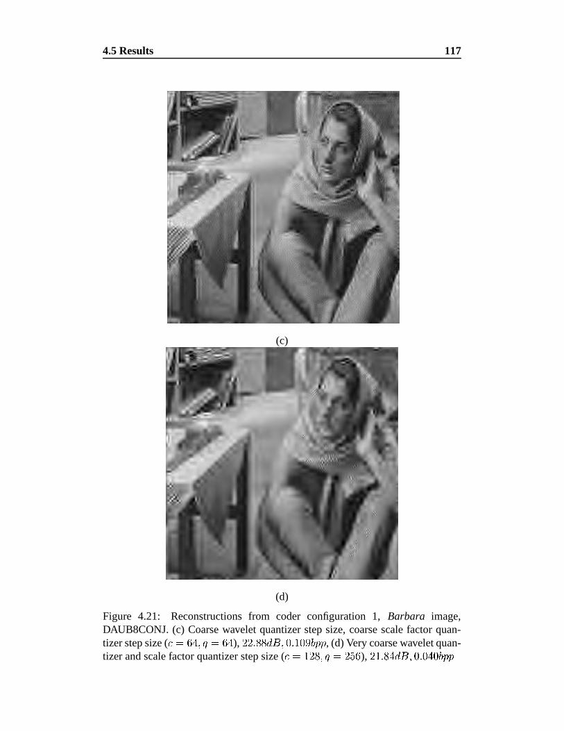
4.5 Results 117
(c)
(d)
Figure 4.21: Reconstructions from coder configuration 1, Barbara image,DAUB8CONJ. (c) Coarse wavelet quantizer step size, coarse scale factor quan-tizer step size ( � � ��� '
����
),� � � � � ' � � ��� � ����� , (d) Very coarse wavelet quan-
tizer and scale factor quantizer step size ( � � ��� ' �
� ���),��� � � � ' � � ��� � � � �
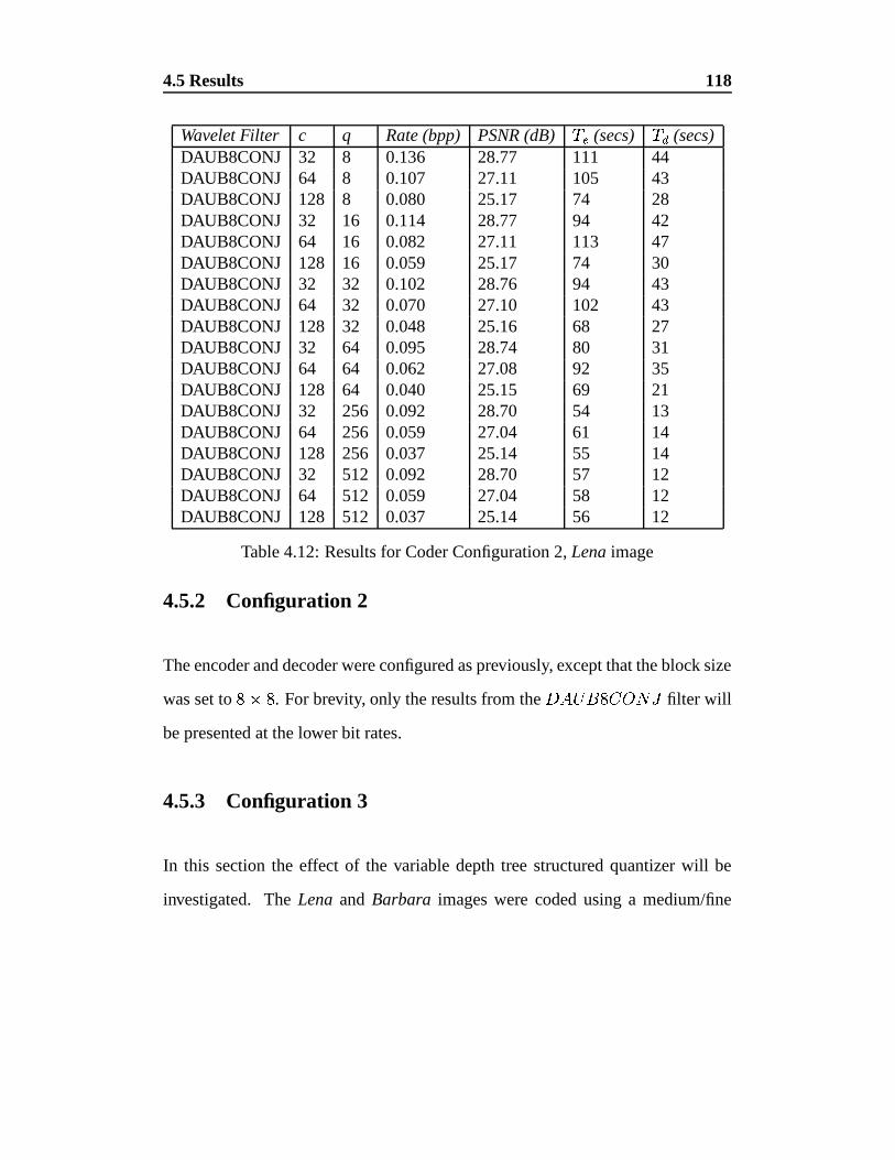
4.5 Results 118
Wavelet Filter c q Rate (bpp) PSNR (dB)�� (secs)
� � (secs)DAUB8CONJ 32 8 0.136 28.77 111 44DAUB8CONJ 64 8 0.107 27.11 105 43DAUB8CONJ 128 8 0.080 25.17 74 28DAUB8CONJ 32 16 0.114 28.77 94 42DAUB8CONJ 64 16 0.082 27.11 113 47DAUB8CONJ 128 16 0.059 25.17 74 30DAUB8CONJ 32 32 0.102 28.76 94 43DAUB8CONJ 64 32 0.070 27.10 102 43DAUB8CONJ 128 32 0.048 25.16 68 27DAUB8CONJ 32 64 0.095 28.74 80 31DAUB8CONJ 64 64 0.062 27.08 92 35DAUB8CONJ 128 64 0.040 25.15 69 21DAUB8CONJ 32 256 0.092 28.70 54 13DAUB8CONJ 64 256 0.059 27.04 61 14DAUB8CONJ 128 256 0.037 25.14 55 14DAUB8CONJ 32 512 0.092 28.70 57 12DAUB8CONJ 64 512 0.059 27.04 58 12DAUB8CONJ 128 512 0.037 25.14 56 12
Table 4.12: Results for Coder Configuration 2, Lena image
4.5.2 Configuration 2
The encoder and decoder were configured as previously, except that the block size
was set to � . For brevity, only the results from the ����� �� ���� filter will
be presented at the lower bit rates.
4.5.3 Configuration 3
In this section the effect of the variable depth tree structured quantizer will be
investigated. The Lena and Barbara images were coded using a medium/fine
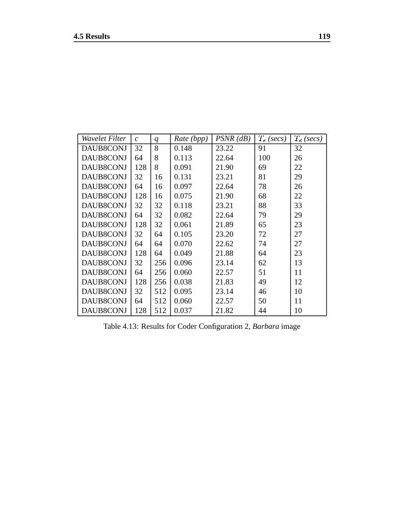
4.5 Results 119
Wavelet Filter c q Rate (bpp) PSNR (dB)�� (secs)
� � (secs)DAUB8CONJ 32 8 0.148 23.22 91 32DAUB8CONJ 64 8 0.113 22.64 100 26DAUB8CONJ 128 8 0.091 21.90 69 22DAUB8CONJ 32 16 0.131 23.21 81 29DAUB8CONJ 64 16 0.097 22.64 78 26DAUB8CONJ 128 16 0.075 21.90 68 22DAUB8CONJ 32 32 0.118 23.21 88 33DAUB8CONJ 64 32 0.082 22.64 79 29DAUB8CONJ 128 32 0.061 21.89 65 23DAUB8CONJ 32 64 0.105 23.20 72 27DAUB8CONJ 64 64 0.070 22.62 74 27DAUB8CONJ 128 64 0.049 21.88 64 23DAUB8CONJ 32 256 0.096 23.14 62 13DAUB8CONJ 64 256 0.060 22.57 51 11DAUB8CONJ 128 256 0.038 21.83 49 12DAUB8CONJ 32 512 0.095 23.14 46 10DAUB8CONJ 64 512 0.060 22.57 50 11DAUB8CONJ 128 512 0.037 21.82 44 10
Table 4.13: Results for Coder Configuration 2, Barbara image
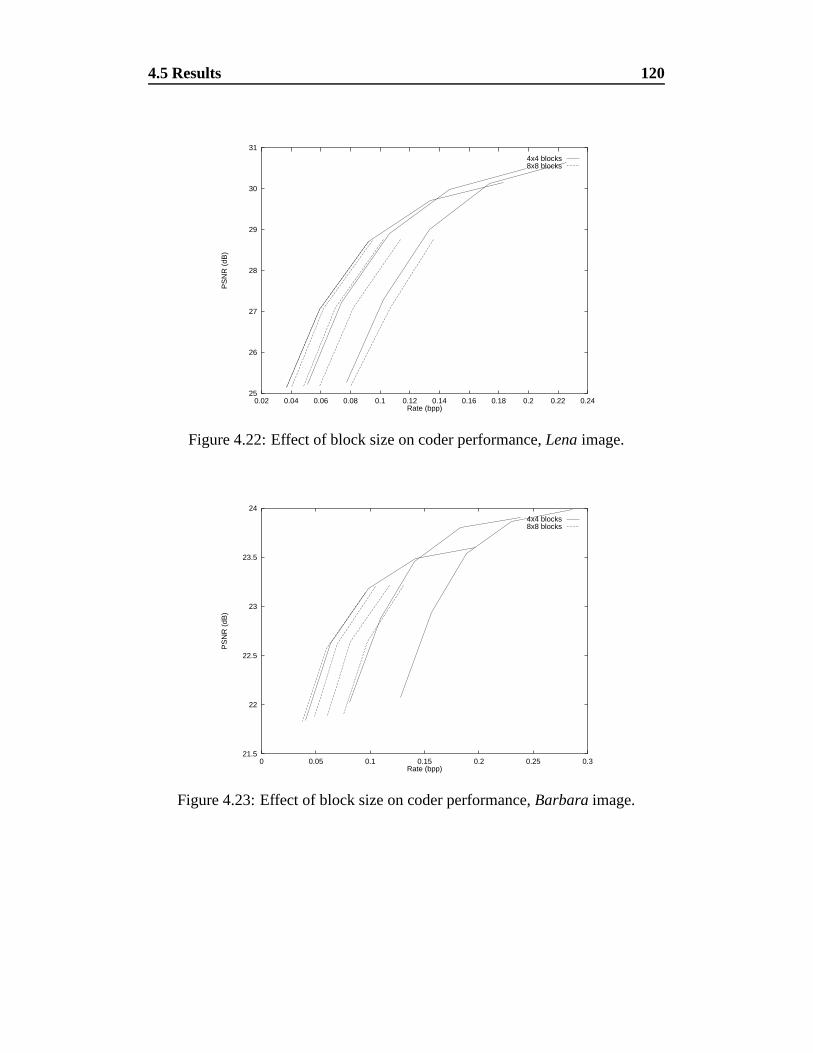
4.5 Results 120
25
26
27
28
29
30
31
0.02 0.04 0.06 0.08 0.1 0.12 0.14 0.16 0.18 0.2 0.22 0.24
PS
NR
(dB
)
Rate (bpp)
4x4 blocks8x8 blocks
Figure 4.22: Effect of block size on coder performance, Lena image.
21.5
22
22.5
23
23.5
24
0 0.05 0.1 0.15 0.2 0.25 0.3
PS
NR
(dB
)
Rate (bpp)
4x4 blocks8x8 blocks
Figure 4.23: Effect of block size on coder performance, Barbara image.
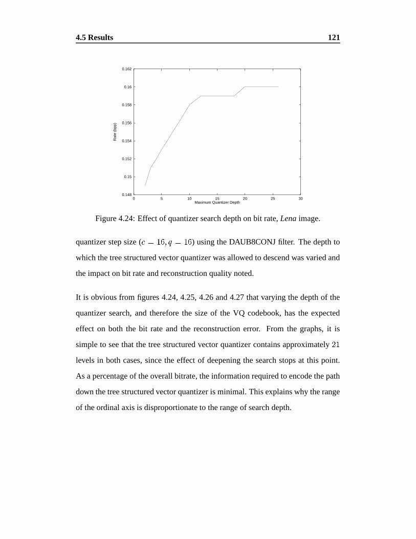
4.5 Results 121
0.148
0.15
0.152
0.154
0.156
0.158
0.16
0.162
0 5 10 15 20 25 30
Rat
e (b
pp)
Maximum Quantizer Depth
Figure 4.24: Effect of quantizer search depth on bit rate, Lena image.
quantizer step size ( � � ��� ' �
���) using the DAUB8CONJ filter. The depth to
which the tree structured vector quantizer was allowed to descend was varied and
the impact on bit rate and reconstruction quality noted.
It is obvious from figures 4.24, 4.25, 4.26 and 4.27 that varying the depth of the
quantizer search, and therefore the size of the VQ codebook, has the expected
effect on both the bit rate and the reconstruction error. From the graphs, it is
simple to see that the tree structured vector quantizer contains approximately���
levels in both cases, since the effect of deepening the search stops at this point.
As a percentage of the overall bitrate, the information required to encode the path
down the tree structured vector quantizer is minimal. This explains why the range
of the ordinal axis is disproportionate to the range of search depth.
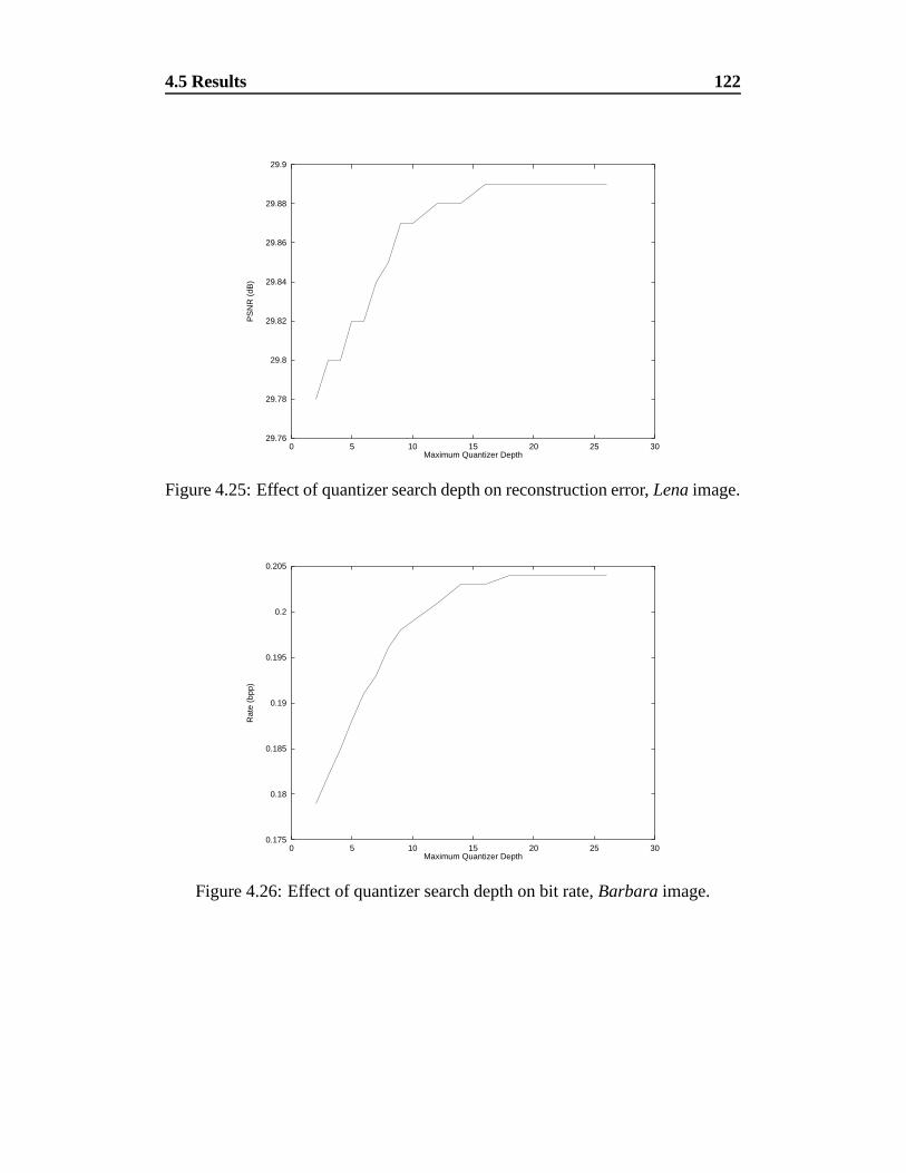
4.5 Results 122
29.76
29.78
29.8
29.82
29.84
29.86
29.88
29.9
0 5 10 15 20 25 30
PS
NR
(dB
)
Maximum Quantizer Depth
Figure 4.25: Effect of quantizer search depth on reconstruction error, Lena image.
0.175
0.18
0.185
0.19
0.195
0.2
0.205
0 5 10 15 20 25 30
Rat
e (b
pp)
Maximum Quantizer Depth
Figure 4.26: Effect of quantizer search depth on bit rate, Barbara image.
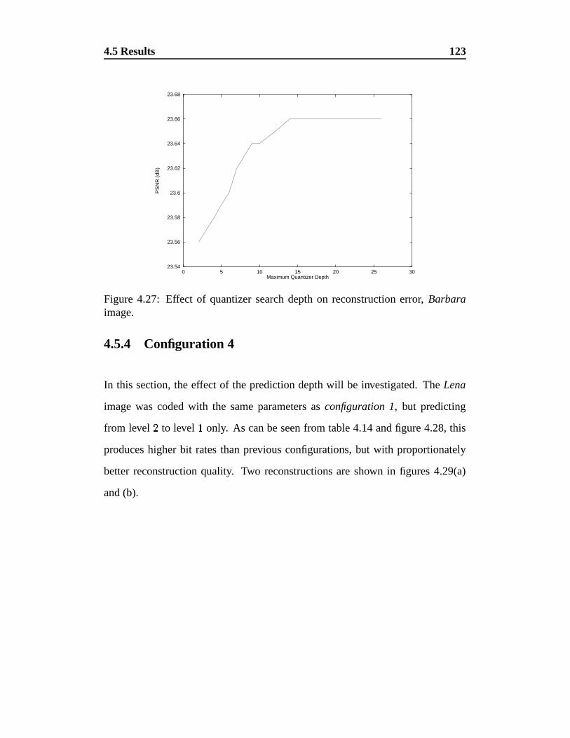
4.5 Results 123
23.54
23.56
23.58
23.6
23.62
23.64
23.66
23.68
0 5 10 15 20 25 30
PS
NR
(dB
)
Maximum Quantizer Depth
Figure 4.27: Effect of quantizer search depth on reconstruction error, Barbaraimage.
4.5.4 Configuration 4
In this section, the effect of the prediction depth will be investigated. The Lena
image was coded with the same parameters as configuration 1, but predicting
from level�
to level�
only. As can be seen from table 4.14 and figure 4.28, this
produces higher bit rates than previous configurations, but with proportionately
better reconstruction quality. Two reconstructions are shown in figures 4.29(a)
and (b).
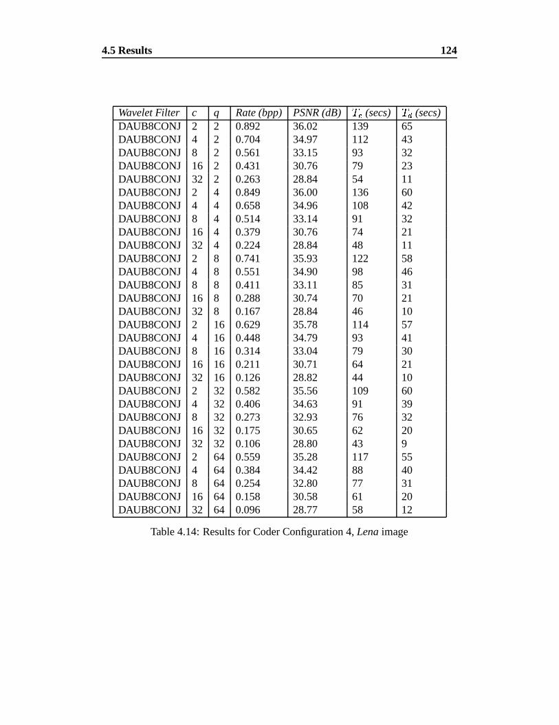
4.5 Results 124
Wavelet Filter c q Rate (bpp) PSNR (dB)�� (secs)
� � (secs)DAUB8CONJ 2 2 0.892 36.02 139 65DAUB8CONJ 4 2 0.704 34.97 112 43DAUB8CONJ 8 2 0.561 33.15 93 32DAUB8CONJ 16 2 0.431 30.76 79 23DAUB8CONJ 32 2 0.263 28.84 54 11DAUB8CONJ 2 4 0.849 36.00 136 60DAUB8CONJ 4 4 0.658 34.96 108 42DAUB8CONJ 8 4 0.514 33.14 91 32DAUB8CONJ 16 4 0.379 30.76 74 21DAUB8CONJ 32 4 0.224 28.84 48 11DAUB8CONJ 2 8 0.741 35.93 122 58DAUB8CONJ 4 8 0.551 34.90 98 46DAUB8CONJ 8 8 0.411 33.11 85 31DAUB8CONJ 16 8 0.288 30.74 70 21DAUB8CONJ 32 8 0.167 28.84 46 10DAUB8CONJ 2 16 0.629 35.78 114 57DAUB8CONJ 4 16 0.448 34.79 93 41DAUB8CONJ 8 16 0.314 33.04 79 30DAUB8CONJ 16 16 0.211 30.71 64 21DAUB8CONJ 32 16 0.126 28.82 44 10DAUB8CONJ 2 32 0.582 35.56 109 60DAUB8CONJ 4 32 0.406 34.63 91 39DAUB8CONJ 8 32 0.273 32.93 76 32DAUB8CONJ 16 32 0.175 30.65 62 20DAUB8CONJ 32 32 0.106 28.80 43 9DAUB8CONJ 2 64 0.559 35.28 117 55DAUB8CONJ 4 64 0.384 34.42 88 40DAUB8CONJ 8 64 0.254 32.80 77 31DAUB8CONJ 16 64 0.158 30.58 61 20DAUB8CONJ 32 64 0.096 28.77 58 12
Table 4.14: Results for Coder Configuration 4, Lena image
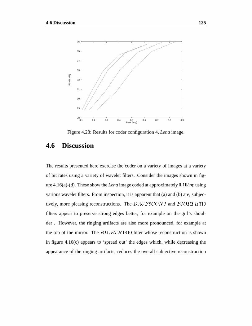
4.6 Discussion 125
28
29
30
31
32
33
34
35
36
0.1 0.2 0.3 0.4 0.5 0.6 0.7 0.8 0.9
PS
NR
(dB
)
Rate (bpp)
Figure 4.28: Results for coder configuration 4, Lena image.
4.6 Discussion
The results presented here exercise the coder on a variety of images at a variety
of bit rates using a variety of wavelet filters. Consider the images shown in fig-
ure 4.16(a)-(d). These show the Lena image coded at approximately� � � ������� using
various wavelet filters. From inspection, it is apparent that (a) and (b) are, subjec-
tively, more pleasing reconstructions. The ��� �� �� �� � and � � � � � ���
filters appear to preserve strong edges better, for example on the girl’s shoul-
der . However, the ringing artifacts are also more pronounced, for example at
the top of the mirror. The � � � � � � � filter whose reconstruction is shown
in figure 4.16(c) appears to ‘spread out’ the edges which, while decreasing the
appearance of the ringing artifacts, reduces the overall subjective reconstruction
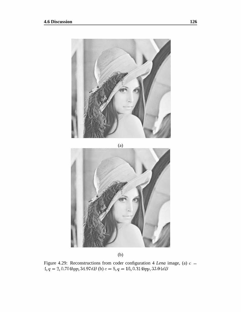
4.6 Discussion 126
(a)
(b)
Figure 4.29: Reconstructions from coder configuration 4 Lena image, (a) � �� ' �
� ' � � � ��� ����� ' � � � � � (b) � � ' �
��� ' � � � ��� � � ' � � ��� �
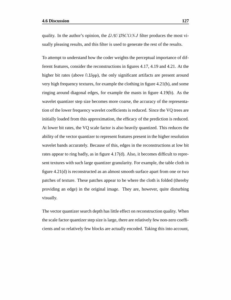
4.6 Discussion 127
quality. In the author’s opinion, the ����� �� ���� filter produces the most vi-
sually pleasing results, and this filter is used to generate the rest of the results.
To attempt to understand how the coder weights the perceptual importance of dif-
ferent features, consider the reconstructions in figures 4.17, 4.19 and 4.21. At the
higher bit rates (above� � � ����� ), the only significant artifacts are present around
very high frequency textures, for example the clothing in figure 4.21(b), and some
ringing around diagonal edges, for example the masts in figure 4.19(b). As the
wavelet quantizer step size becomes more coarse, the accuracy of the representa-
tion of the lower frequency wavelet coefficients is reduced. Since the VQ trees are
initially loaded from this approximation, the efficacy of the prediction is reduced.
At lower bit rates, the VQ scale factor is also heavily quantized. This reduces the
ability of the vector quantizer to represent features present in the higher resolution
wavelet bands accurately. Because of this, edges in the reconstructions at low bit
rates appear to ring badly, as in figure 4.17(d). Also, it becomes difficult to repre-
sent textures with such large quantizer granularity. For example, the table cloth in
figure 4.21(d) is reconstructed as an almost smooth surface apart from one or two
patches of texture. These patches appear to be where the cloth is folded (thereby
providing an edge) in the original image. They are, however, quite disturbing
visually.
The vector quantizer search depth has little effect on reconstruction quality. When
the scale factor quantizer step size is large, there are relatively few non-zero coeffi-
cients and so relatively few blocks are actually encoded. Taking this into account,
4.6 Discussion 128
the difference in reconstruction between using a full depth search and using a re-
stricted search is significant, giving an increase of approximately� � ��� � for an
increase of� � � ��� � � � . There is almost no difference in the encoding and decoding
times. In order to see the effect that the vector quantizer has on reconstructed im-
age quality, compare figures 4.17 (c) and (d). The wavelet quantizer granularity
is identical in both figures. In figure 4.17(c) the VQ scale factor quantizer granu-
larity is relatively small, while in (d) the step size is so large that all coefficients
quantize to zero, effectively disabling the VQ portion of the coder. From inspec-
tion, it is easy to see that the VQ portion of the coder does increase subjective
quality of strong features, for example around the eyes and the edge of the mirror.
The wavelet transforms used in this work perform wrap around at the image edges.
From inspection of the reconstructed images at the edges, it is apparent that this
may not be the most suitable choice. For example, in figure 4.17(c), there is
heavy ringing along the top edge and the top of the left hand edge. This ap-
pears to be where there is a large difference between the grey scale values on the
opposing limits of the image. This creates an edge when wrapped around and
consequently produces the disturbing ringing artifacts. A possible simple solution
to this would be to employ periodic extension or repetition of the data instead of
wrapping around.
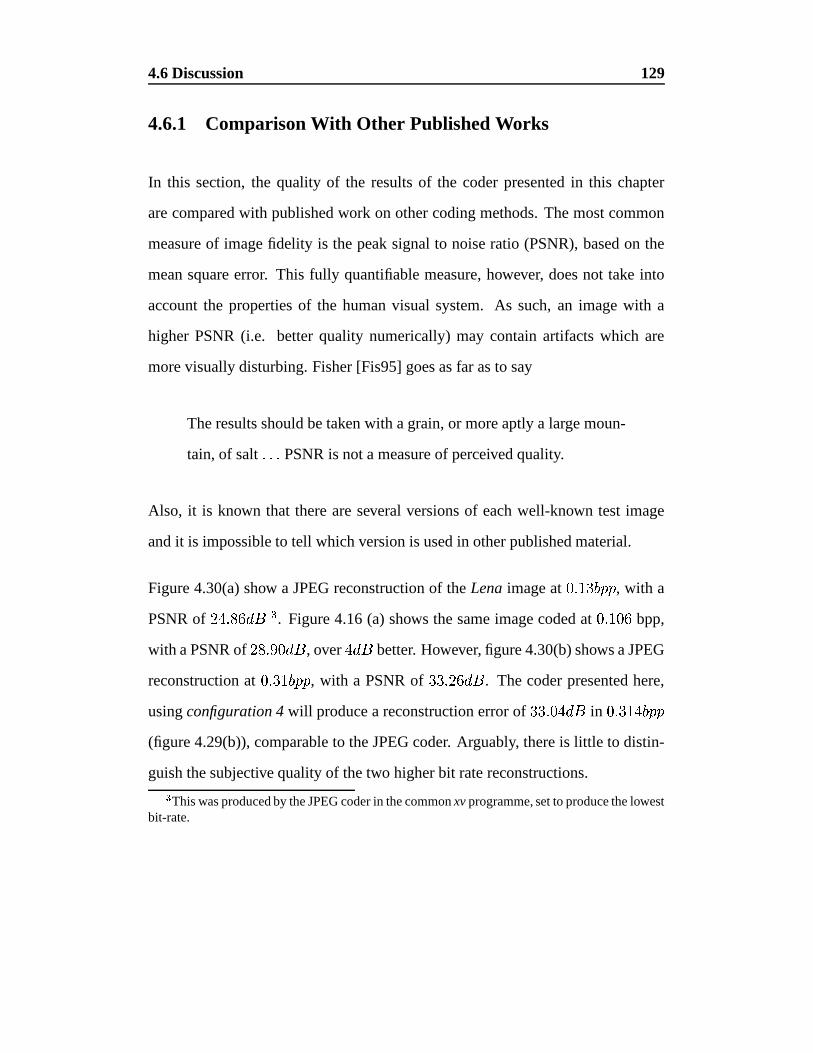
4.6 Discussion 129
4.6.1 Comparison With Other Published Works
In this section, the quality of the results of the coder presented in this chapter
are compared with published work on other coding methods. The most common
measure of image fidelity is the peak signal to noise ratio (PSNR), based on the
mean square error. This fully quantifiable measure, however, does not take into
account the properties of the human visual system. As such, an image with a
higher PSNR (i.e. better quality numerically) may contain artifacts which are
more visually disturbing. Fisher [Fis95] goes as far as to say
The results should be taken with a grain, or more aptly a large moun-
tain, of salt � � � PSNR is not a measure of perceived quality.
Also, it is known that there are several versions of each well-known test image
and it is impossible to tell which version is used in other published material.
Figure 4.30(a) show a JPEG reconstruction of the Lena image at� � � � � � , with a
PSNR of� � � � � �
. Figure 4.16 (a) shows the same image coded at� � ����� bpp,
with a PSNR of� � � � � , over
� � better. However, figure 4.30(b) shows a JPEG
reconstruction at� � � ����� , with a PSNR of � � ��� � . The coder presented here,
using configuration 4 will produce a reconstruction error of � � ��� � in� � � � �����
(figure 4.29(b)), comparable to the JPEG coder. Arguably, there is little to distin-
guish the subjective quality of the two higher bit rate reconstructions.�
This was produced by the JPEG coder in the common xv programme, set to produce the lowestbit-rate.
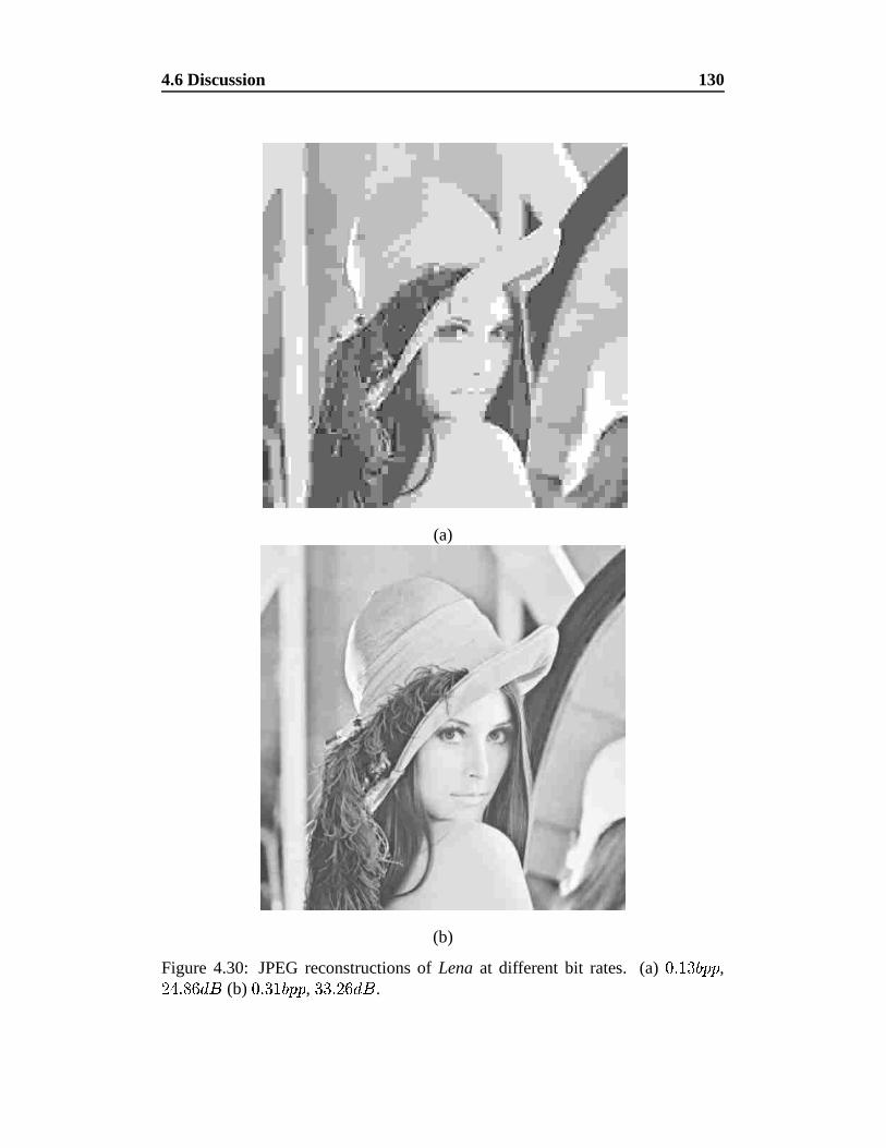
4.6 Discussion 130
(a)
(b)
Figure 4.30: JPEG reconstructions of Lena at different bit rates. (a)� � � ����� ,
� � � � � (b)� � � ����� , � � � � � .
4.6 Discussion 131
Table 4.15 compares the reconstruction results for the coder presented here with
currently published works. It is apparent from the table that the algorithm pre-
sented here performs as well as or better than all the comparative methods at low
bit rates. Shapiro’s EZW coder [Sha93] remains the benchmark for all image cod-
ing algorithms at low rates. The coder presented here matches Shapiro’s coder
closely at the lower bit rates for the Lena image. The Barbara image used by
Shapiro appears to be slightly different from the one used here, although the re-
sults are included for completeness. The Boats and Barbara images are more
difficult to code than the Lena image because of the greater degree of texture and
prevalence of high frequency artifacts.
The coder presented here does not work well at high bit rates and the encoding
of the lower frequency bands of the wavelet transform may be the cause. On the
other hand, at low bit rates the reconstructions do not appear to suffer from the
highly visually disturbing artifacts usually associated with block based coders.
The artifacts that are introduced at lower bit rates appear to be caused by the ring-
ing of the wavelet filters around edges, since altering the wavelet filters alters the
character of the artifacts. A post-processing algorithm, such as an adaptation of
the adaptive thresholding algorithm in [GLGO94], may well reduce these artifacts
and increase the visual quality of the reconstructed images. It also seems likely
that a more symmetric set of orientation bands, i.e. ones not based on a separable
transform, may well be better adapted to human visual system properties. Design
of such a set of filters is a highly complex task, however.�
The Barbara image used by Shapiro appears to be different to the one used here.
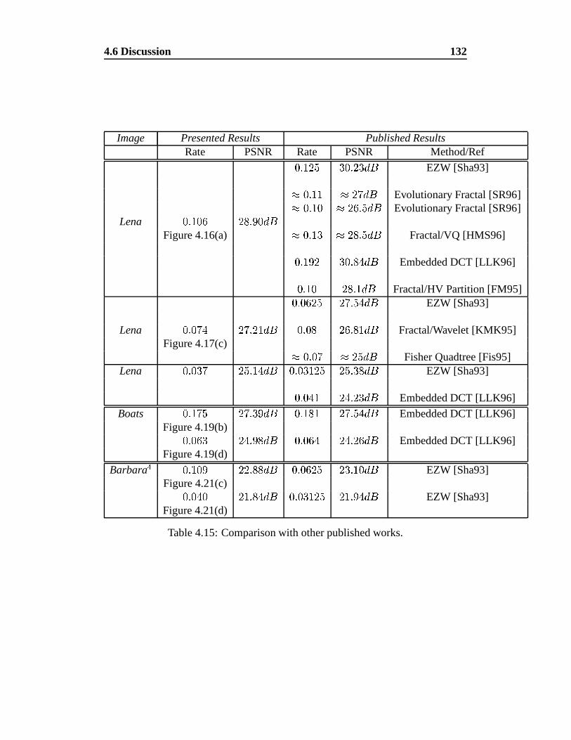
4.6 Discussion 132
Image Presented Results Published ResultsRate PSNR Rate PSNR Method/Ref
� � ��� � � � � � EZW [Sha93]
� � � � � � � � � Evolutionary Fractal [SR96]� � � ��� � ��� � � � Evolutionary Fractal [SR96]
Lena� � ����� � � � � �
Figure 4.16(a) � � � � � � � � � Fractal/VQ [HMS96]
� � � � � � � � � Embedded DCT [LLK96]
� � ��� � � � � Fractal/HV Partition [FM95]� � ��� � � � � � � � � EZW [Sha93]
Lena� � � � � � � � ��� � � � � ��� � � � Fractal/Wavelet [KMK95]
Figure 4.17(c)� � � � � � � � � Fisher Quadtree [Fis95]
Lena� � � � � � � � � � � � � � � � � � � � � EZW [Sha93]
� � ��� � � � � � � Embedded DCT [LLK96]
Boats� � � � � � � � � � � � � � � � � � � � Embedded DCT [LLK96]
Figure 4.19(b)� � ��� � � � � � � � ����� � � � ��� � Embedded DCT [LLK96]Figure 4.19(d)
Barbara� � � ��� � � � � � � � � ��� � � � � ��� � EZW [Sha93]
Figure 4.21(c)� � ��� � ��� � � � � � � ��� � ��� � � � � EZW [Sha93]Figure 4.21(d)
Table 4.15: Comparison with other published works.
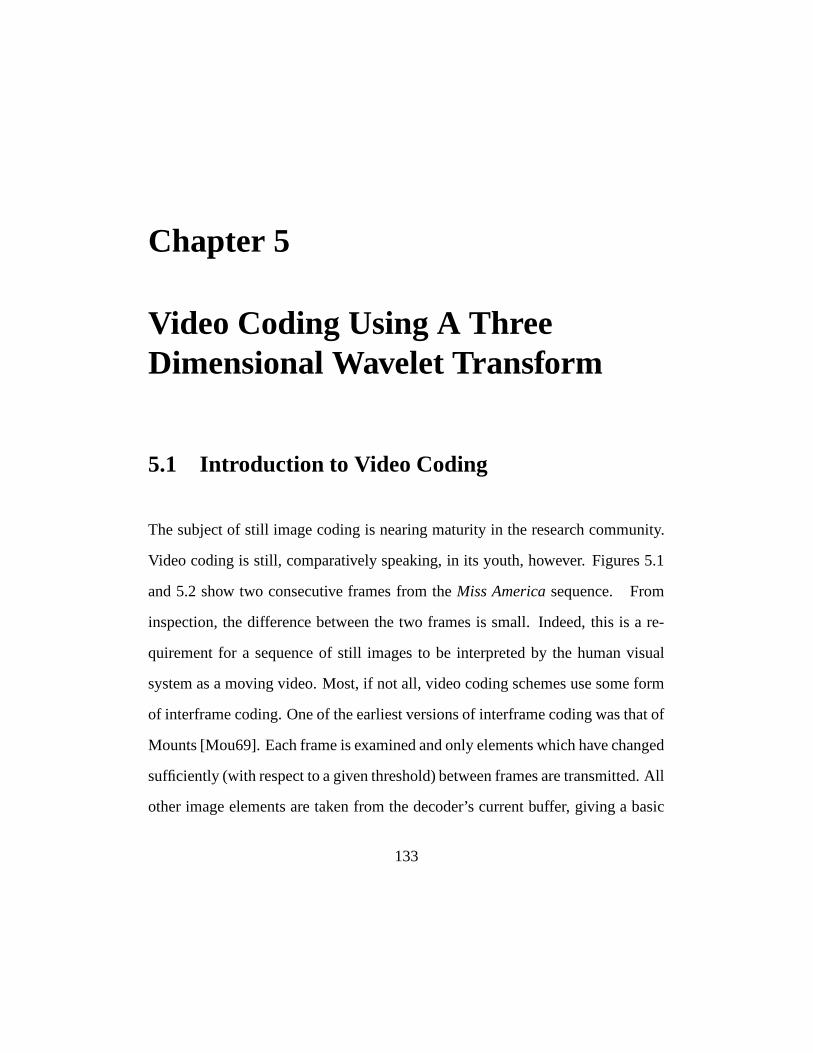
Chapter 5
Video Coding Using A ThreeDimensional Wavelet Transform
5.1 Introduction to Video Coding
The subject of still image coding is nearing maturity in the research community.
Video coding is still, comparatively speaking, in its youth, however. Figures 5.1
and 5.2 show two consecutive frames from the Miss America sequence. From
inspection, the difference between the two frames is small. Indeed, this is a re-
quirement for a sequence of still images to be interpreted by the human visual
system as a moving video. Most, if not all, video coding schemes use some form
of interframe coding. One of the earliest versions of interframe coding was that of
Mounts [Mou69]. Each frame is examined and only elements which have changed
sufficiently (with respect to a given threshold) between frames are transmitted. All
other image elements are taken from the decoder’s current buffer, giving a basic
133
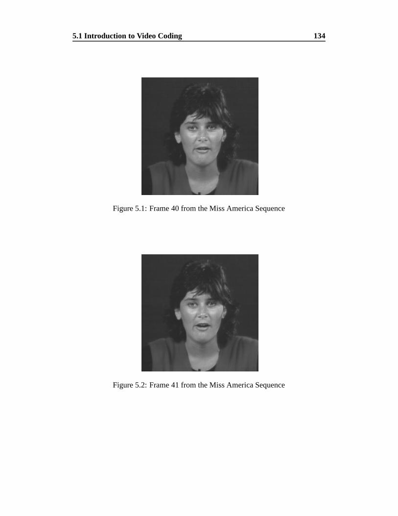
5.1 Introduction to Video Coding 134
Figure 5.1: Frame 40 from the Miss America Sequence
Figure 5.2: Frame 41 from the Miss America Sequence
5.1 Introduction to Video Coding 135
form of prediction [Cla95]. In predictive coding, previously coded pixels are used
as a context for encoding the current pixel. The predictor is analogous to the two
dimensional case, except that temporal neighbours are also included. As an ex-
tension to this, transform domain predictors have also been used in video coding
[Cla85]. In these, the current and previous frames are transformed and the pre-
diction is applied to the transform coefficients. This has the advantage that, given
the correct choice of transform and quantization, many of the coefficients will be
zero, enabling simple entropy coding.
Many of the more modern video coding schemes try to predict the motion of vi-
sually important features. In this way, it is argued, the encoder can spend more
bits on the visually important features of the sequence. Indeed, the encoder and
decoder both have the same prediction algorithm to predict where features may
move to in the next frame. If the prediction is correct, very little data need to be
sent. However, if the prediction is wrong, information must be sent which will
allow the decoder to correct its prediction. The predictions are usually based on
some form of model. If the features or the motion do not fit the model, the pre-
diction errors will be large and occur frequently. This will drive up the bit rate
or reduce the quality of the reconstructed sequence. The most widely used pre-
diction method in video coding algorithms is motion compensation. Motion com-
pensation attempts to predict where a group of pixels (be they a feature or some
geometric patch) will move to in the next frame. By sending such a motion vector,
the decoder can just apply the motion vector to the block in frame � to produce
5.1 Introduction to Video Coding 136
the moved block in frame � � � . The motion vectors produced by this method are
often a very limited subset of the possible motions. If the full range of motion was
allowed, the information required to encode the parameters of each motion would
probably outweigh the information saved in the prediction. As with any predictive
system, motion compensation is accompanied by transmitting a difference signal,
to reduce the error rate and prevent instability. For example, the current industry
standard video coding algorithm, MPEG [LeG92] [Tek95], uses motion compen-
sation. Motion compensation does have its problems, though. Motion vectors are
usually limited to simple translations to reduce computation. Obviously, this sim-
plification does not always fit the data, causing errors. The video coding research
community is currently very active in improving motion compensation schemes.
Multiscale (hierarchical) compensation and generalized compensation, where the
motion is not so restricted, are both current research topics [SMP97]. A more ro-
bust method would perhaps not use such a simple model and would not, therefore,
be limited to certain features and motions. There are the widely accepted concepts
of features, motion, direction and velocity. Combinations of these concepts will
determine whether something is required to be coded accurately or can be ignored.
For example, a small feature moving very quickly will be largely ignored by the
human visual system [Wat88]. Some form of transform which separates the im-
age data into classes of features and non-features and which further separates the
features into their respective velocities and directions would therefore provide an
ideal base for a video compression algorithm.
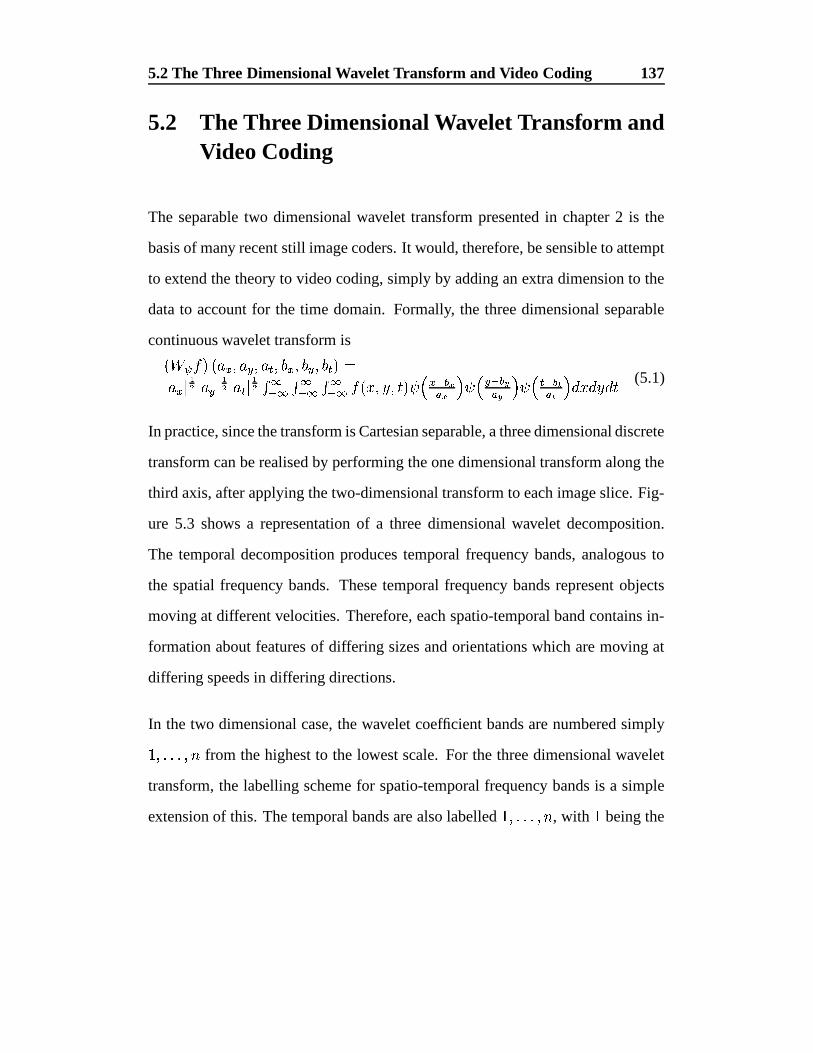
5.2 The Three Dimensional Wavelet Transform and Video Coding 137
5.2 The Three Dimensional Wavelet Transform andVideo Coding
The separable two dimensional wavelet transform presented in chapter 2 is the
basis of many recent still image coders. It would, therefore, be sensible to attempt
to extend the theory to video coding, simply by adding an extra dimension to the
data to account for the time domain. Formally, the three dimensional separable
continuous wavelet transform is� � �
� � � / $ ' / ' / � ' � $ ' � ' � � � �� / $ � � / � � / � �
� �� � � �� � � �� � � ��� ' � ' � � � � $ ��� �� � � � �����
� � � � � �����
� � � � � � � � (5.1)
In practice, since the transform is Cartesian separable, a three dimensional discrete
transform can be realised by performing the one dimensional transform along the
third axis, after applying the two-dimensional transform to each image slice. Fig-
ure 5.3 shows a representation of a three dimensional wavelet decomposition.
The temporal decomposition produces temporal frequency bands, analogous to
the spatial frequency bands. These temporal frequency bands represent objects
moving at different velocities. Therefore, each spatio-temporal band contains in-
formation about features of differing sizes and orientations which are moving at
differing speeds in differing directions.
In the two dimensional case, the wavelet coefficient bands are numbered simply� ' � � � ' � from the highest to the lowest scale. For the three dimensional wavelet
transform, the labelling scheme for spatio-temporal frequency bands is a simple
extension of this. The temporal bands are also labelled� ' � � � ' � , with
�being the
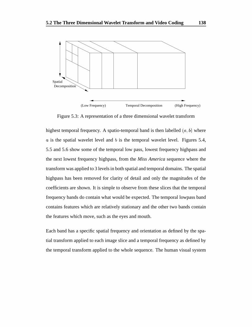
5.2 The Three Dimensional Wavelet Transform and Video Coding 138
Spatial
Temporal Decomposition
Decomposition
(Low Frequency) (High Frequency)
Figure 5.3: A representation of a three dimensional wavelet transform
highest temporal frequency. A spatio-temporal band is then labelled � / ' � � where
/ is the spatial wavelet level and�
is the temporal wavelet level. Figures 5.4,
5.5 and 5.6 show some of the temporal low pass, lowest frequency highpass and
the next lowest frequency highpass, from the Miss America sequence where the
transform was applied to 3 levels in both spatial and temporal domains. The spatial
highpass has been removed for clarity of detail and only the magnitudes of the
coefficients are shown. It is simple to observe from these slices that the temporal
frequency bands do contain what would be expected. The temporal lowpass band
contains features which are relatively stationary and the other two bands contain
the features which move, such as the eyes and mouth.
Each band has a specific spatial frequency and orientation as defined by the spa-
tial transform applied to each image slice and a temporal frequency as defined by
the temporal transform applied to the whole sequence. The human visual system
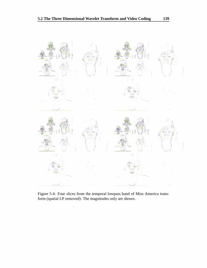
5.2 The Three Dimensional Wavelet Transform and Video Coding 139
Figure 5.4: Four slices from the temporal lowpass band of Miss America trans-form (spatial LP removed). The magnitudes only are shown.
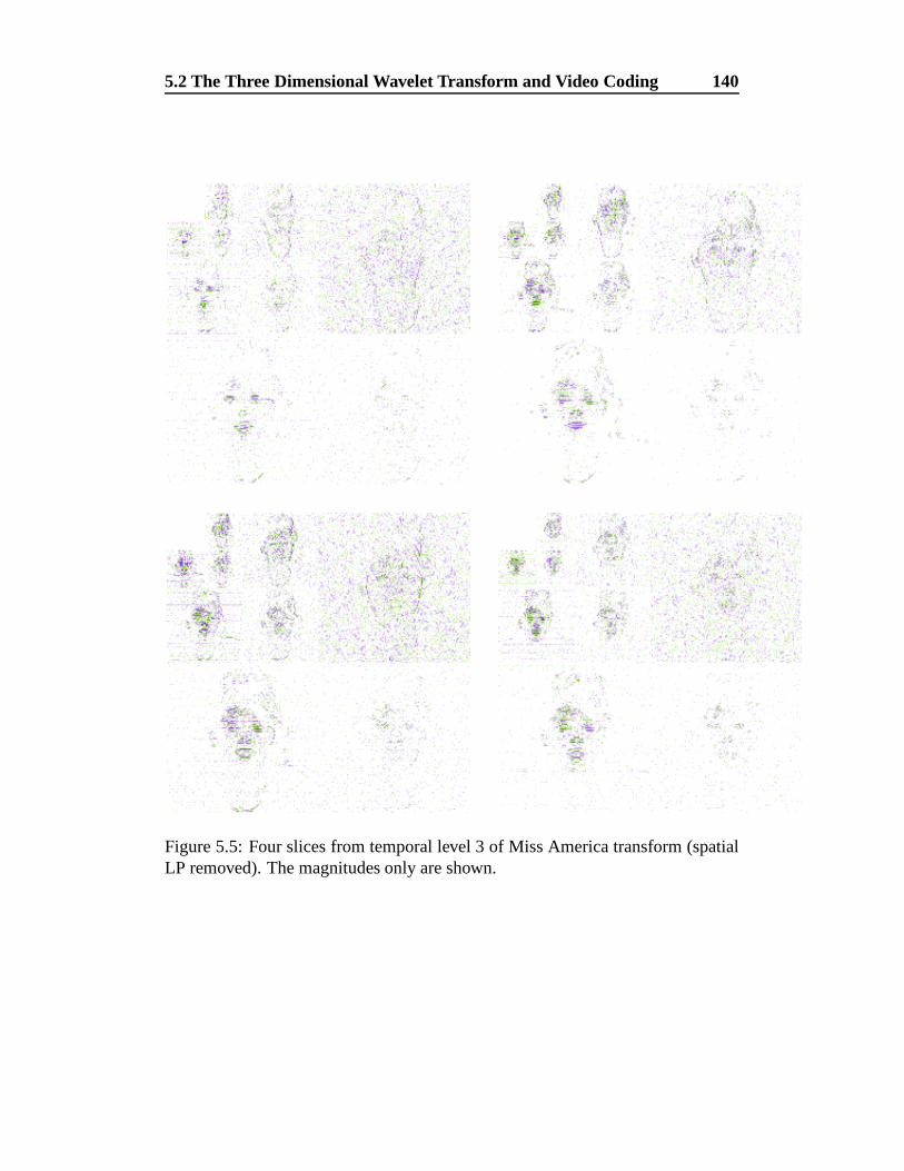
5.2 The Three Dimensional Wavelet Transform and Video Coding 140
Figure 5.5: Four slices from temporal level 3 of Miss America transform (spatialLP removed). The magnitudes only are shown.
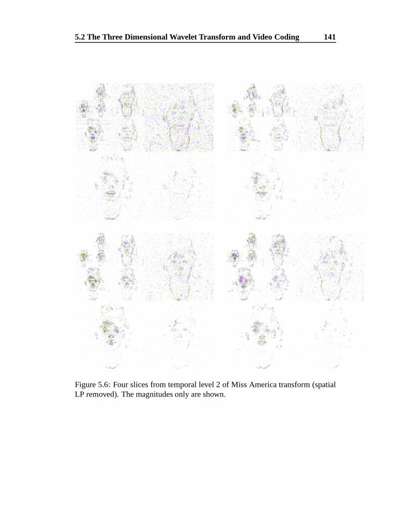
5.2 The Three Dimensional Wavelet Transform and Video Coding 141
Figure 5.6: Four slices from temporal level 2 of Miss America transform (spatialLP removed). The magnitudes only are shown.
5.2 The Three Dimensional Wavelet Transform and Video Coding 142
is only responsive to certain spatio-temporal frequencies [Wat88]. Indeed, high
spatio-temporal frequencies are generally ignored by the human visual system.
Therefore, it is possible to eliminate entirely certain spatio-temporal frequency
bands and code others depending on their importance in the human visual sys-
tem model. In its simplest form, a three dimensional wavelet video coder could
simply linearly quantize and entropy code each spatio-temporal frequency band.
The quantizations and coding parameters would be dependent upon the spatio-
temporal frequency band. In the following tests, the original image sequence was
appended to itself in reverse in order to preserve the temporal continuity at the
sequence ends, since a normal video stream is mostly temporally continuous.
5.2.1 A linear quantizer based wavelet video coder
The test sequence is constructed and the 2 dimensional wavelet transform applied
to each image frame in turn, decomposing to a specified level, followed by a one
dimensional wavelet transform applied in the temporal direction, again to a spec-
ified level. Then, given a quantizer bin size, , the encoding proceeds by linearly
quantizing the spatio-temporal highpass with one quantizer and the spatial and
temporal lowpass bands with another, finer quantizer. The quantizer bin numbers
are entropy coded using an order zero arithmetic coder. The highest frequency
temporal highpass level is ignored entirely, since the high spatio-temporal fre-
quency data in this band are largely ignored by the human visual system. This
extremely simple method produces some remarkably good results, detailed next.
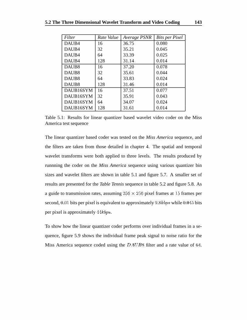
5.2 The Three Dimensional Wavelet Transform and Video Coding 143
Filter Rate Value Average PSNR Bits per PixelDAUB4 16 36.75 0.080DAUB4 32 35.21 0.045DAUB4 64 33.39 0.025DAUB4 128 31.14 0.014DAUB8 16 37.20 0.078DAUB8 32 35.61 0.044DAUB8 64 33.83 0.024DAUB8 128 31.46 0.014DAUB16SYM 16 37.51 0.077DAUB16SYM 32 35.91 0.043DAUB16SYM 64 34.07 0.024DAUB16SYM 128 31.61 0.014
Table 5.1: Results for linear quantizer based wavelet video coder on the MissAmerica test sequence
The linear quantizer based coder was tested on the Miss America sequence, and
the filters are taken from those detailed in chapter 4. The spatial and temporal
wavelet transforms were both applied to three levels. The results produced by
runnning the coder on the Miss America sequence using various quantizer bin
sizes and wavelet filters are shown in table 5.1 and figure 5.7. A smaller set of
results are presented for the Table Tennis sequence in table 5.2 and figure 5.8. As
a guide to transmission rates, assuming� ��� � � ���
pixel frames at� �
frames per
second,� � � � bits per pixel is equivalent to approximately
� � � � � � while� � ��� � bits
per pixel is approximately��� � ��� � .
To show how the linear quantizer coder performs over individual frames in a se-
quence, figure 5.9 shows the individual frame peak signal to noise ratio for the
Miss America sequence coded using the � ��� filter and a rate value of���
.
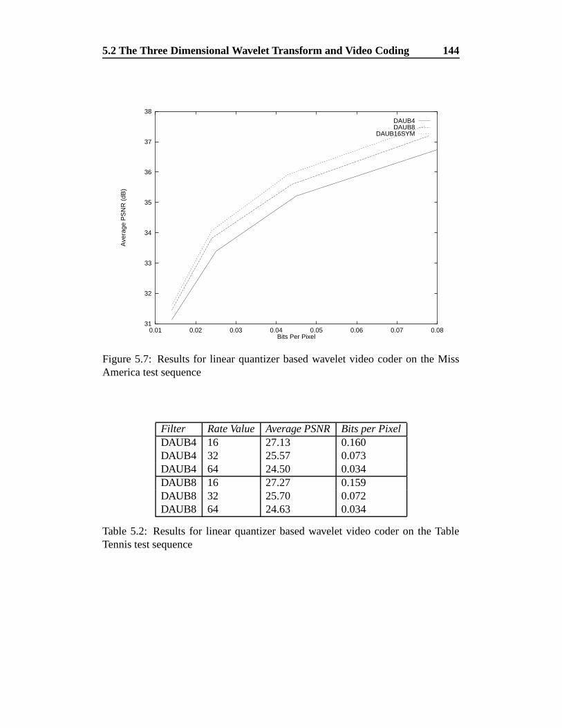
5.2 The Three Dimensional Wavelet Transform and Video Coding 144
31
32
33
34
35
36
37
38
0.01 0.02 0.03 0.04 0.05 0.06 0.07 0.08
Ave
rage
PS
NR
(dB
)
Bits Per Pixel
DAUB4DAUB8
DAUB16SYM
Figure 5.7: Results for linear quantizer based wavelet video coder on the MissAmerica test sequence
Filter Rate Value Average PSNR Bits per PixelDAUB4 16 27.13 0.160DAUB4 32 25.57 0.073DAUB4 64 24.50 0.034DAUB8 16 27.27 0.159DAUB8 32 25.70 0.072DAUB8 64 24.63 0.034
Table 5.2: Results for linear quantizer based wavelet video coder on the TableTennis test sequence
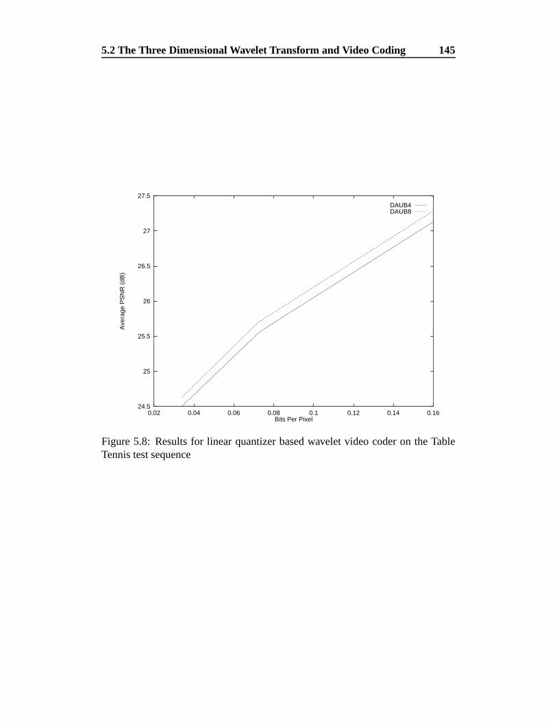
5.2 The Three Dimensional Wavelet Transform and Video Coding 145
24.5
25
25.5
26
26.5
27
27.5
0.02 0.04 0.06 0.08 0.1 0.12 0.14 0.16
Ave
rage
PS
NR
(dB
)
Bits Per Pixel
DAUB4DAUB8
Figure 5.8: Results for linear quantizer based wavelet video coder on the TableTennis test sequence
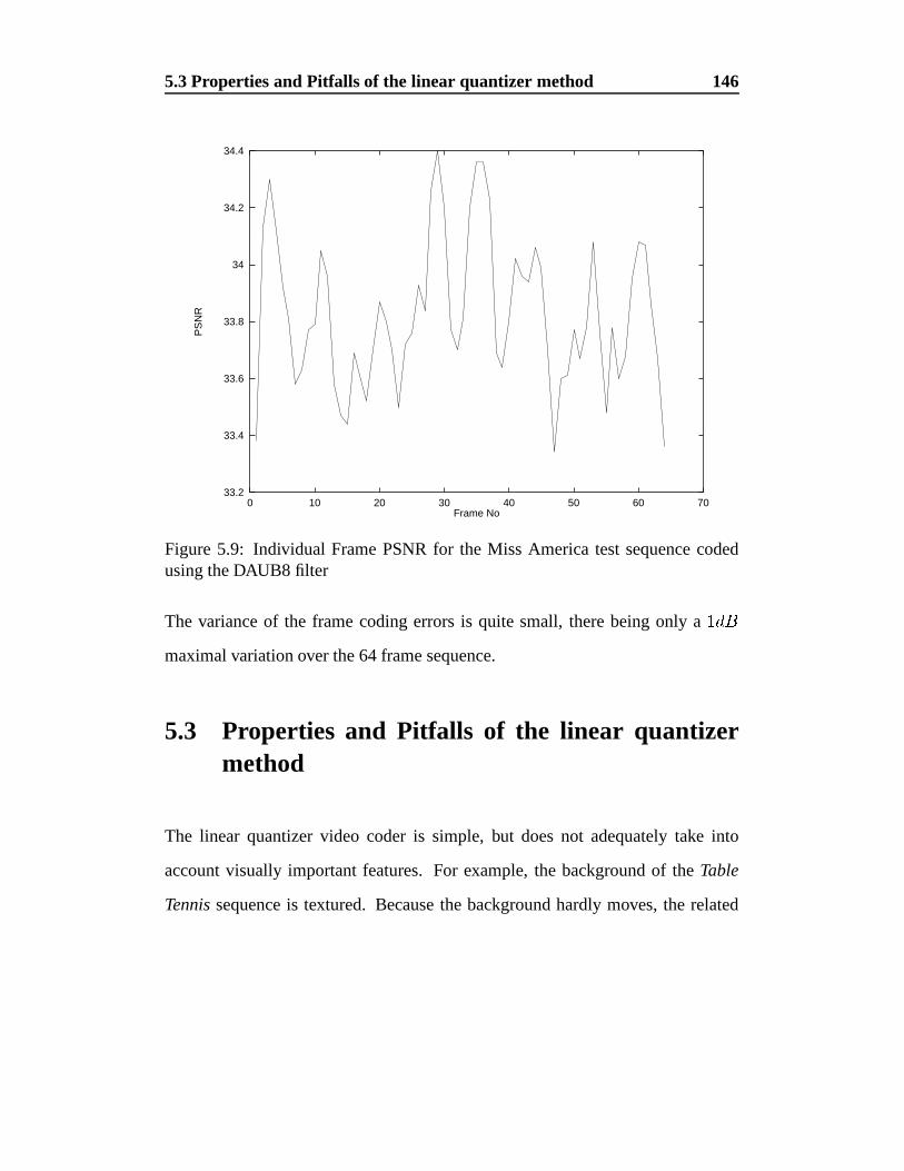
5.3 Properties and Pitfalls of the linear quantizer method 146
33.2
33.4
33.6
33.8
34
34.2
34.4
0 10 20 30 40 50 60 70
PS
NR
Frame No
Figure 5.9: Individual Frame PSNR for the Miss America test sequence codedusing the DAUB8 filter
The variance of the frame coding errors is quite small, there being only a� �
maximal variation over the 64 frame sequence.
5.3 Properties and Pitfalls of the linear quantizermethod
The linear quantizer video coder is simple, but does not adequately take into
account visually important features. For example, the background of the Table
Tennis sequence is textured. Because the background hardly moves, the related
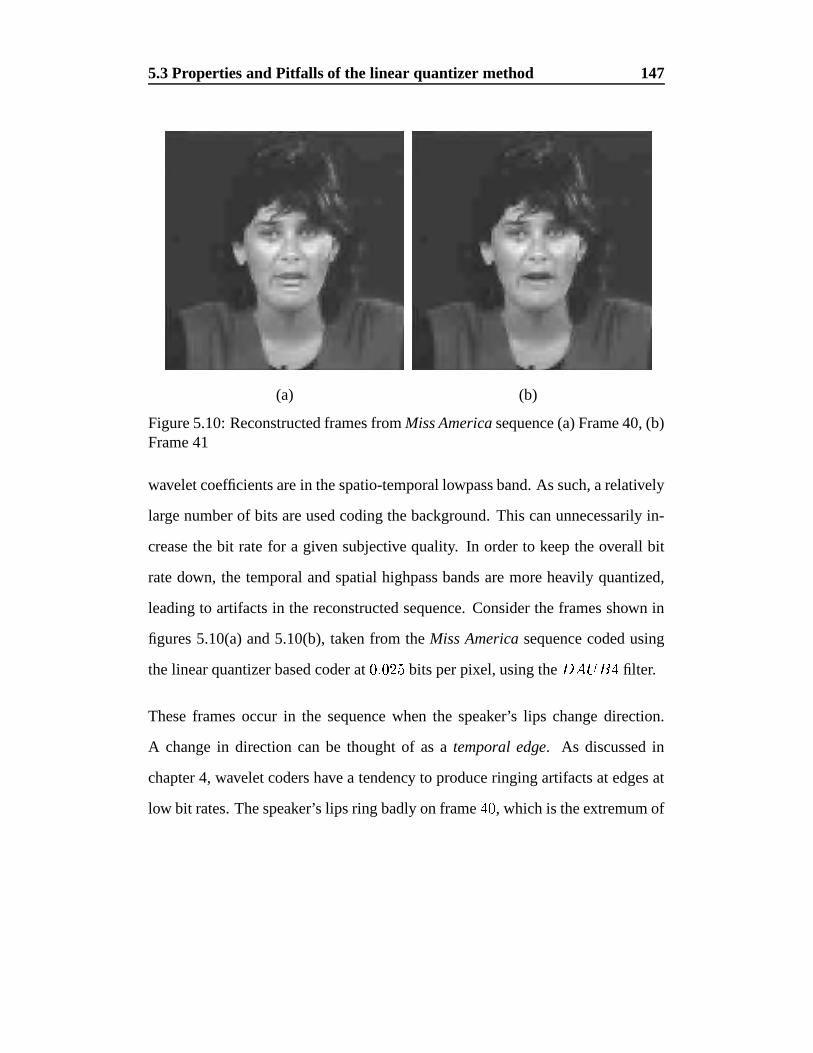
5.3 Properties and Pitfalls of the linear quantizer method 147
(a) (b)
Figure 5.10: Reconstructed frames from Miss America sequence (a) Frame 40, (b)Frame 41
wavelet coefficients are in the spatio-temporal lowpass band. As such, a relatively
large number of bits are used coding the background. This can unnecessarily in-
crease the bit rate for a given subjective quality. In order to keep the overall bit
rate down, the temporal and spatial highpass bands are more heavily quantized,
leading to artifacts in the reconstructed sequence. Consider the frames shown in
figures 5.10(a) and 5.10(b), taken from the Miss America sequence coded using
the linear quantizer based coder at� � � � � bits per pixel, using the � ��� � filter.
These frames occur in the sequence when the speaker’s lips change direction.
A change in direction can be thought of as a temporal edge. As discussed in
chapter 4, wavelet coders have a tendency to produce ringing artifacts at edges at
low bit rates. The speaker’s lips ring badly on frame� �
, which is the extremum of
5.4 A VQ based Video Coding Algorithm 148
the lip movement and the system recovers on frame� �
. A method that accounts
for more of the structure and features of the underlying transform is required.
5.4 A VQ based Video Coding Algorithm
It is widely known in the image coding community that a well designed vector
quantizer should outperform a linear quantizer [LBG80]. A two dimensional vec-
tor quantizer encodes patches of an image. By extension, a three dimensional
vector quantizer will encode patches of an image in a certain time interval. That
is, the vector quantization representative vectors will consist of features that pass
across the image patch during the time window. This has obvious similarities
to the decomposition provided by the three dimensional wavelet transform. To
begin, the video image sequence is decomposed by the spatio-temporal wavelet
transform. In all the tests that follow, the transform was applied to three spatial
and three temporal levels. The highest temporal frequency band is not coded. As
stated previously, the high spatio-temporal frequency data present in this band is
relatively perceptually unimportant to the human visual system. The temporal
lowpass band and all spatial lowpass bands are quantized with a uniform, linear
scalar quantizer with a relatively small bin size. The spatial lowpass contains con-
tinuous tone sections of image and the temporal lowpass contains features which,
relatively speaking, do not move during the sequence. Scalar quantizing this data
with a relatively fine quantizer allows for a good overall impression of the se-
quence to be produced with no detail. The detail from the sequence is eminently
5.4 A VQ based Video Coding Algorithm 149
suitable for vector quantization. In order to produce a generalised coder, a general
purpose vector quantization codebook must be created. To produce this code-
book, a variety of image sequences was scanned and appropriately sized cuboids
of data extracted from the appropriate wavelet coefficients. In these tests, the vec-
tors were� � � � �
pixels and were accumulated from spatio-temporal wavelet
level � ' � . As in the still image coder presented in section 4.4, two tree struc-
tured vector quantizers are used: one for the horizontally and vertically oriented
data and one for the diagonally oriented data. The trees contain vectors which are
stored in a canonical orientation. The time-reverse, per-pixel negation and negated
time reverse of any vectors are also stored. Time reversal allows for objects mov-
ing in either direction and per-pixel negation is used to ensure that the generated
codebook has a zero vector. If the energy of any particular block extracted is be-
low a given threshold, it is treated as noise and does not contribute to the vector
accumulation. Different thresholds are used for the H-V and D trees.
Given a vector quantizer codebook, spatio-temporal bands � ' � , � � ' � � , � ' � � and
� � ' � are vector quantized and the VQ indices are entropy coded using an order
zero arithmetic coder. Recall from section 2.4.3 that the discrete wavelet transform
is directly equivalent to a multiresolution analysis. Recall also, equation 2.18,
repeated here for convenience. Assume that! � � � � � � � is a multiresolution
analysis. Then� � ! � � � � �
�� � ! � �� � (5.2)
Moving to the frequency domain , this equation states that if a function� � ! �
5.4 A VQ based Video Coding Algorithm 150
has a frequency of � , then the functions contained in the subspace! � �� will have
frequency� � . Define
to be a velocity. Then, a translation at velocity
of a
complex exponential is simply
��� �� $ � � � � � ��� �
$ � � � � � �(5.3)
from which � � �
� �� (5.4)
So, for a given spatial band � and temporal band�, the velocity of the features
in spatio-temporal band ��� ' � � will be twice that of features in � ��
� ' � � . Now,
features present in spatio-temporal band � � ' � will be similar to those present
in spatio-temporal band � ' � except that they will be moving twice as fast. In
order to account for the velocity difference, the quantizer vectors are dyadically
downsampled in the temporal direction. Then the downsampled codebooks are
used to encode spatio-temporal bands � � ' � and � � ' � � . Again, a simple, order zero
arithmetic coder acts as the entropy coder. Figure 5.11 shows a block diagram of
the coder.
In all the following tests, the H-V codebook contains� ���
vectors and the diagonal
codebook� �
. The subsampled codebooks contain the same number of vectors as
the original codebooks. These values are fairly arbitrary but investigation showed
that these produced better results than other values in the range� �
to� � � �
vectors
per codebook. Since the VQ codebook is fixed, the rate control comes about from
the variation of the quantization of the temporal lowpass bands.
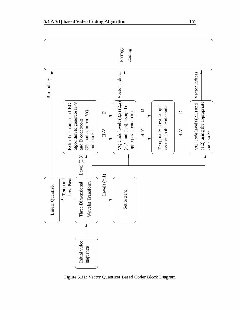
5.4 A VQ based Video Coding Algorithm 151
Initi
al v
ideo
sequ
ence
Thr
ee D
imen
sion
al
Wav
elet
Tra
nsfo
rm
Set t
o ze
roLev
els
(*,1
)
Lin
ear
Qua
ntiz
er
Tem
pora
lL
ow P
ass
Lev
el (
3,3)
VQ
Cod
e le
vels
(3,
3) (
2,2)
(3,2
) an
d (1
,3),
usi
ng th
e ap
prop
riat
e co
debo
ok
H-V
D
Tem
pora
lly d
owns
ampl
eve
ctor
s in
the
code
book
s
H-V
D
(1,2
) us
ing
the
appr
opri
ate
code
book
s
VQ
Cod
e le
vels
(2,
3) a
nd
H-V
D
Vec
tor
Indi
ces
Vec
tor
Indi
ces
Bin
Ind
ices
Ent
ropy
Cod
ing
Ext
ract
dat
a an
d ru
n L
BG
algo
rith
m to
gen
erat
e H
-Van
d D
cod
eboo
ksO
R lo
ad c
omm
on V
Qco
debo
oks.
Figure 5.11: Vector Quantizer Based Coder Block Diagram
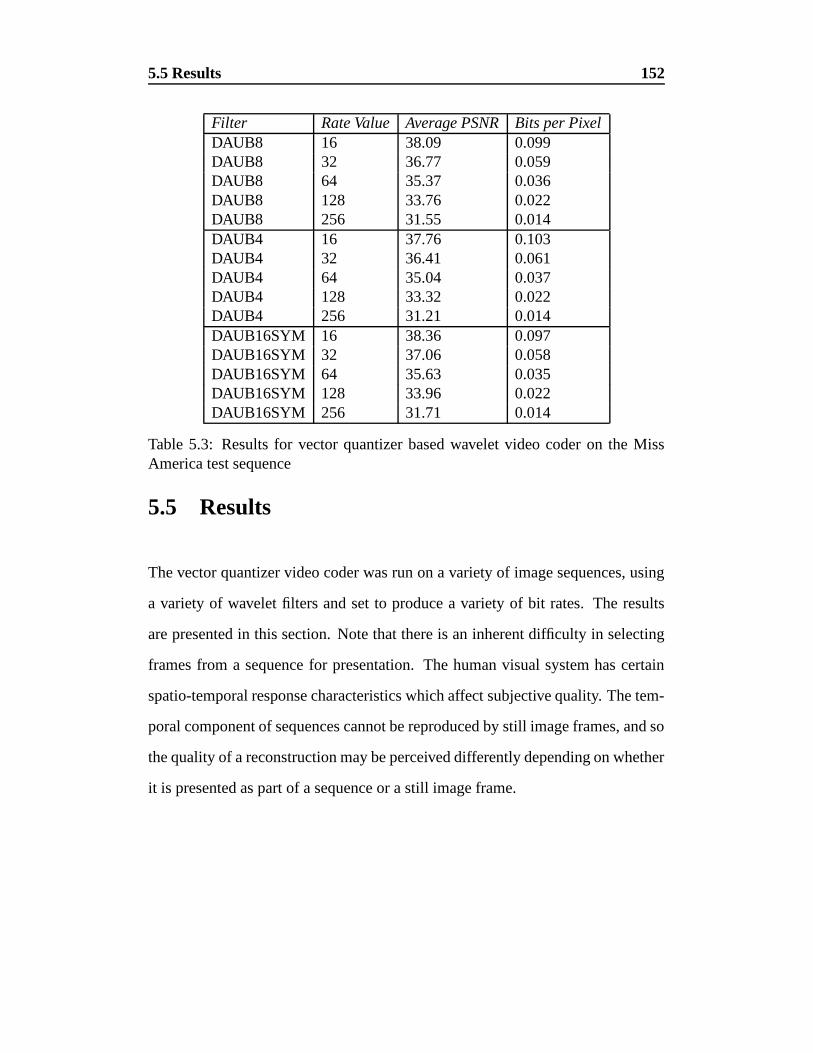
5.5 Results 152
Filter Rate Value Average PSNR Bits per PixelDAUB8 16 38.09 0.099DAUB8 32 36.77 0.059DAUB8 64 35.37 0.036DAUB8 128 33.76 0.022DAUB8 256 31.55 0.014DAUB4 16 37.76 0.103DAUB4 32 36.41 0.061DAUB4 64 35.04 0.037DAUB4 128 33.32 0.022DAUB4 256 31.21 0.014DAUB16SYM 16 38.36 0.097DAUB16SYM 32 37.06 0.058DAUB16SYM 64 35.63 0.035DAUB16SYM 128 33.96 0.022DAUB16SYM 256 31.71 0.014
Table 5.3: Results for vector quantizer based wavelet video coder on the MissAmerica test sequence
5.5 Results
The vector quantizer video coder was run on a variety of image sequences, using
a variety of wavelet filters and set to produce a variety of bit rates. The results
are presented in this section. Note that there is an inherent difficulty in selecting
frames from a sequence for presentation. The human visual system has certain
spatio-temporal response characteristics which affect subjective quality. The tem-
poral component of sequences cannot be reproduced by still image frames, and so
the quality of a reconstruction may be perceived differently depending on whether
it is presented as part of a sequence or a still image frame.
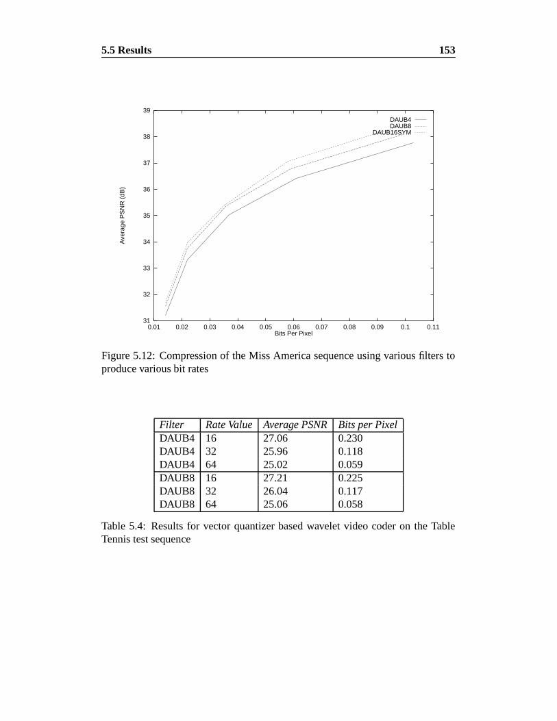
5.5 Results 153
31
32
33
34
35
36
37
38
39
0.01 0.02 0.03 0.04 0.05 0.06 0.07 0.08 0.09 0.1 0.11
Ave
rage
PS
NR
(dB
)
Bits Per Pixel
DAUB4DAUB8
DAUB16SYM
Figure 5.12: Compression of the Miss America sequence using various filters toproduce various bit rates
Filter Rate Value Average PSNR Bits per PixelDAUB4 16 27.06 0.230DAUB4 32 25.96 0.118DAUB4 64 25.02 0.059DAUB8 16 27.21 0.225DAUB8 32 26.04 0.117DAUB8 64 25.06 0.058
Table 5.4: Results for vector quantizer based wavelet video coder on the TableTennis test sequence
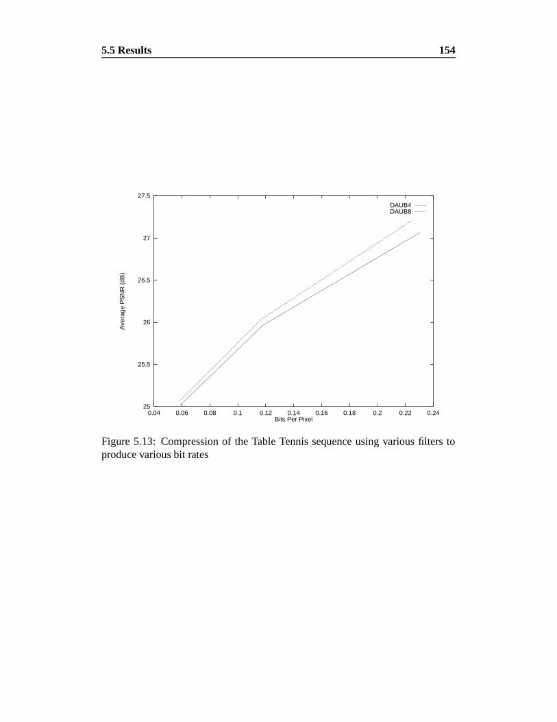
5.5 Results 154
25
25.5
26
26.5
27
27.5
0.04 0.06 0.08 0.1 0.12 0.14 0.16 0.18 0.2 0.22 0.24
Ave
rage
PS
NR
(dB
)
Bits Per Pixel
DAUB4DAUB8
Figure 5.13: Compression of the Table Tennis sequence using various filters toproduce various bit rates
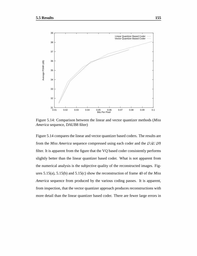
5.5 Results 155
31
32
33
34
35
36
37
38
39
0.01 0.02 0.03 0.04 0.05 0.06 0.07 0.08 0.09 0.1
Ave
rage
PS
NR
(dB
)
Bits Per Pixel
Linear Quantizer Based CoderVector Quantizer Based Coder
Figure 5.14: Comparison between the linear and vector quantizer methods (MissAmerica sequence, DAUB8 filter)
Figure 5.14 compares the linear and vector quantizer based coders. The results are
from the Miss America sequence compressed using each coder and the ��� ��
filter. It is apparent from the figure that the VQ based coder consistently performs
slightly better than the linear quantizer based coder. What is not apparent from
the numerical analysis is the subjective quality of the reconstructed images. Fig-
ures 5.15(a), 5.15(b) and 5.15(c) show the reconstruction of frame� �
of the Miss
America sequence from produced by the various coding passes. It is apparent,
from inspection, that the vector quantizer approach produces reconstructions with
more detail than the linear quantizer based coder. There are fewer large errors in
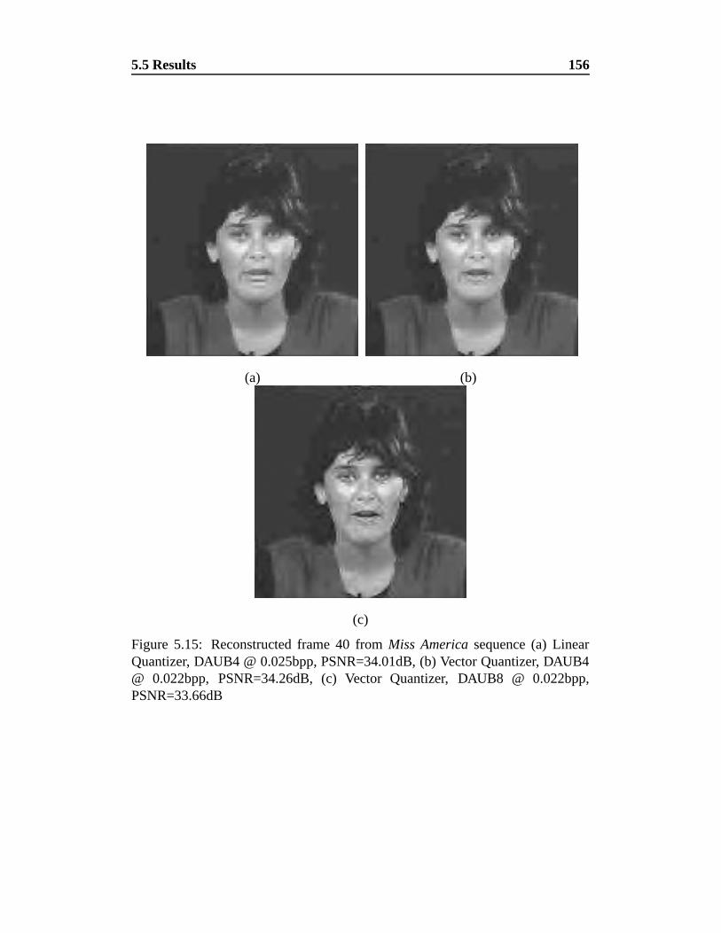
5.5 Results 156
(a) (b)
(c)
Figure 5.15: Reconstructed frame 40 from Miss America sequence (a) LinearQuantizer, DAUB4 @ 0.025bpp, PSNR=34.01dB, (b) Vector Quantizer, DAUB4@ 0.022bpp, PSNR=34.26dB, (c) Vector Quantizer, DAUB8 @ 0.022bpp,PSNR=33.66dB
5.6 Comparison with other video coding techniques 157
the VQ reconstruction and any artifacts appear to have a higher frequency. There
is still some ringing near edges, but this could be reduced with a simple post-
processing algorithm. Since the artifacts are of a higher frequency, peak signal to
noise ratio is not a particularly useful measure of subjective quality. Indeed, the
vector quantizer, by its very nature, will attempt to preserve more detail than its
scalar counterpart. This is easily seen by comparing the eyes in figures 5.15(a),
5.15(b) and 5.15(c). The VQ based coder produces better defined eyes in both
cases, and a much better defined mouth in figure 5.15(c) in spite of the change in
the filter used. To aid inspection, the left eye has been extracted from the original
frame and all three of the reconstructions. A scaled up version of each is shown
in figure 5.16. From these, it is obvious that the vector quantizer coder preserves
detail better than the linear quantizer coder. Also, despite a lower PSNR, the vec-
tor quantizer coder using the ��� � filter preserves detail even better than the
same coder using the ��� � � filter.
5.6 Comparison with other video coding techniques
It is problematic to compare video coding schemes from results presented in the
literature. This is because research groups seem to use different measures, some-
times not fully specifying them. For example, some results are presented as bits
per second, without specifying frame size or rate. In order to provide a basis for
comparison, where full details are not provided, it is assumed that the sequence is
in CIF format [Cla95]. All data from the relevant research papers are converted

5.6 Comparison with other video coding techniques 158
(a) (b)
(c) (d)
Figure 5.16: Detail from the eye area of frame 40 from reconstructions of theMiss America sequence. (a) Original (b) Linear quantizer coder, ����� � filter(c) Vector quantizer coder, ����� � filter (d) Vector quantizer coder, ����� filter.
5.6 Comparison with other video coding techniques 159
into bits per pixel, so that a simple comparison may be performed. In [CRA96],
the authors present a coder based on a combination of DPCM and vector quan-
tization methods. They produce results on QCIF (i.e.� ��� � � � �
pixel). Any
comparison drawn from these results will not be perfect, since the resolution of
the sequence plays an important role in determining the final quality of the recon-
structed sequence. The authors produce results on the monochrome Miss America
sequence at� �
frames per second. They achieve approximately � � � � at approx-
imately� � � bpp and approximately � � � � at approximately
� � ��� bits per pixel.
These values are approximate because the authors only provide average PSNR
and bit rate per frame graphs, not tables. The algorithm presented here, using the
� ��� filter achieves � � � � at
� � � � bpp and � � � � � at
� � � � � bpp. These
values represent gains of approximately� � in each case.
Podilchuk, Jayant and Farvardin [PJF95] presented a subband video coder based
on a combination of tree structured vector quantization and ADPCM techniques.
Their tree structured vector quantizer differs from the one presented in chapter 4
in that it only contains the data presented to it and so becomes unbalanced very
quickly. The authors’ node-splitting construction ensures that Euclidean close
vectors share long common prefixes on their tree path codewords. This allows
them to use inter-block noiseless coding to take advantage of temporal and spa-
tial correlations. Any common prefixes were Huffman coded. Their results are
presented in a very odd way; they simply state that
� � � the Miss America sequence looks very good encoded at 128kbps
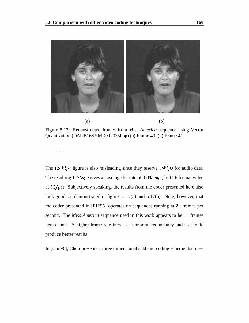
5.6 Comparison with other video coding techniques 160
(a) (b)
Figure 5.17: Reconstructed frames from Miss America sequence using VectorQuantization (DAUB16SYM @ 0.035bpp) (a) Frame 40, (b) Frame 41
� � �
The� � � ��� � figure is also misleading since they reserve
� � � ��� � for audio data.
The resulting� � � � ��� � gives an average bit rate of
� � � � � � � (for CIF format video
at � � � � ). Subjectively speaking, the results from the coder presented here also
look good, as demonstrated in figures 5.17(a) and 5.17(b). Note, however, that
the coder presented in [PJF95] operates on sequences running at �
frames per
second. The Miss America sequence used in this work appears to be���
frames
per second. A higher frame rate increases temporal redundancy and so should
produce better results.
In [Cho96], Chou presents a three dimensional subband coding scheme that uses
5.7 Discussion 161
a model of the human visual system. His model produces either Just Noticable
Distortion or Minimally Noticable Distortion profiles from a model of the vi-
sual system. This allows the author’s system to allocate bits to those coefficients
which are more perceptually important. His temporal frequency decomposition
uses the Haar wavelet and so only consists of two frames. The larger span of
the temporal frequency decompostition presented here (which is the length of the
underlying wavelet filter) provides a simple model of the sort of spatio-temporal
frequencies that are important in the human visual system model. Indeed, Chou’s
results (which are, again, QCIF resolution at��� � � � ) give approximately �
� at� � � � � � � and
� � at� � ��������� . The coder presented here, working on
� ��� � � ���
sequences and using the ��� �� ��� � � � filter, will produce � � ��� � at
� � � � �����
and � � � � at� � � � � ����� . Even taking into consideration the resolution differ-
ence, these results are still quite impressive.
5.7 Discussion
The results presented here are comparable with, and often better than, other coding
schemes which are published at this time. Most current video coding schemes use
motion compensation. Motion compensation schemes have problems, as detailed
earlier in this chapter. For example, the motion vectors are often approximated
to simple translations, and this often does not mimic reality. Furthermore, be-
cause motion compensation relies on prediction, it can be upset by changes in the
sequence which do not adhere to the relatively simple model that the prediction
5.7 Discussion 162
imposes. A smooth video sequence will have many image elements that move
only slightly between frames and the predictive nature of the motion compensa-
tion scheme will cope well with this. However, abruptly changing motions or
flashing images do not fit the temporal prediction model and will not be handled
well by a motion compensation scheme. The three dimensional wavelet trans-
form, however, does not impose such a restrictive model on the data. The energy
compaction and decorrelation properties of the transform mean that most of the
information is concentrated in the lower frequency bands. Any rapid, non-smooth
changes will produce data in the higher frequency bands. These high frequency
components can be dealt with by the coder when necessary and the coder will de-
grade gracefully. The video coders presented here do suffer from some problems.
The selection of the underlying wavelet filter affects the reconstructed image qual-
ity and bit rate. It appears that the longer symmetric filters give better results, both
numerically and subjectively, probably due to their smoother nature. Longer filters
also decorrelate the spatial data better, providing more scope for prediction and
entropy coding. The simple linear quantizer would benefit from a more intelligent
quantization scheme. Indeed, a Lloyd-Max quantizer or even several quantizers
of differing granularities could be used for each spatio-temporal frequency band.
This would allow the coder to take perceptual importance into account more pre-
cisely. The vector quantizer based coder could also benefit from a more robust
VQ scheme. Normalising the vectors and sending a scale factor, as in the still
image coder presented in chapter 3, would probably increase the quality of the
reconstructed images. In summary, these results are very encouraging, but more

5.7 Discussion 163
work is needed to produce an optimised coder.
Chapter 6
Discussion, Conclusions and FutureWork
The work in this thesis is concerned with the compression of still image and video
compression using wavelets and the design of coders utilising the properties of
the transform.
6.1 Conclusions
The analysis of the basis generated by iterated function schemes in chapter 2 is
original. It demonstrates that, as defined by Jacquin [Jac90], fractal image com-
pression cannot achieve perfect reconstruction of arbitrary signals. Furthermore,
the dyadic averaging and downsampling preferred by fractal methods was shown
to be sub-optimal. The optimal basis for fractal image compression was derived
and it was shown that, up to a shift, the wavelet basis is the ideal basis for fractal
164
6.1 Conclusions 165
image compression. Furthermore, it was shown that using an orthonormal wavelet
transform would remove the need for iteration and, therefore, the constraint on the
contractivity of the mappings.
The new paradigm for image coding introduced in chapter 3 builds directly on
the analysis of chapter 2. The relation between fractal and wavelet methods is
made concrete by the coder presented. The prediction down the wavelet tree is
exactly as specified in the basis analysis. In order to compactly represent errors,
the KL transform was used to create a codebook of error correction vectors which
is complete on the space of errors. The preservation of local feature orientation
was shown to be important by introducing a crude orientation estimate which is
used to exclude vectors from the search for the minimal error prediction. The
results produced by the coder are subjectively good at medium to high bit rates.
There are no blocking artifacts, which are normally associated with block based
image coders. Since the prediction occurs in the wavelet domain, any blocking
artifacts will occur in the wavelet domain. When the inverse wavelet filter is ap-
plied, the quantization noise which created the blocking artifacts is ‘spread out’
over the length of the wavelet filter. This produces the higher frequency artifacts
apparent at low bit rates. These artifacts, while still disturbing, are less preceptu-
ally important to the human visual system. The fractal-wavelet combination has
thus been demonstrated to be a useful framework for predictive coding. Some of
the problems associated with the system were addressed in the next chapter.
The conventional wavelet transform groups multiresolution features into similar
6.1 Conclusions 166
orientations. The oriented wavelet transform presented in chapter 4 further refines
this selectivity by producing 6 complex valued sub-bands. Even though it does not
use the conventional quadrature mirror filter design, the transform retains many of
its desirable properties. The tree structured vector quantizer presented in chapter 4
overcomes many of the limitations exhibited by earlier TSVQs. Indeed, it is fully
on-line and there is no distinction between a training phase and a use phase. The
inclusion of the distortion measure and representative vector at each node allows
for variable rate coding or coding to a given error specification. The quantizer is
relatively computationally simple, since the error at any node is calculated implic-
itly, rather than explicitly. The extra storage requirements of this method are far
outweighed by the decrease in computation time. The results presented for the
TSVQ, while limited, demonstrate its ability to match theoretical coding limits
down to 1 bit per vector. The speed of the quantizer, coupled with the variable
rate property make it ideal for image coding applications.
The results presented in chapter 4 are among the most promising in the image
coding community. The PSNR distortion measure has often been shown to be a
less than perfect measure of image quality. However, the coder presented here
matches or exceeds the numerical results from all available research. It is impos-
sible subjectively to compare image quality since the specifics of printing cannot
be taken into account. Subjectively, the image reconstructions in chapter 4 are
more pleasing than many other coding schemes, especially at very low bit rates.
The extension of predictive wavelet coding to video sequences is relatively straight-
6.2 Limitations and Further Work 167
forward. Chapter 5 presented a video coding scheme based around the three di-
mensional, Cartesian separable wavelet transform and the tree structured vector
quantizer. An analysis of the spatio-temporal features present in each wavelet
sub-band allows the codebook design to take into account both feature orientation
and velocity. The final coding results again are among the best reported to date.
The artifacts introduced at very low bit rates are disturbing, but not as disturbing
as the heavy blocking artifacts introduced by, say, MPEG encoders.
6.2 Limitations and Further Work
All the work in this thesis in concerned with greyscale images. An obvious ex-
tension to each coding scheme would be to encode colour images and sequences.
The extension should be relatively straightforward. The colour images could be
represented in the� � !
colour space. The coders presented here would operate,
almost unchanged on the�
plane of these images. The � and!
planes could be
coded separately, to re-introduce colour.
For the still image coder, the simplistic nature of the quantization of the lower
frequency wavelet coefficients is a major drawback. The most obvious alternative
for encoding the low frequency coefficients is a vector quantization scheme. This
would almost certainly only apply to the detail bands, leaving the lowpass band to
be scalar quantized, as it is presently.
The effect that the underlying wavelet filter has on the reconstruction quality has
6.2 Limitations and Further Work 168
been clearly demonstrated by the results presented in chapter 4. For example, the
filter � � � � � � � always performs significantly worse than the others. This
could be attributed to the fact that this filter pair has a longer analysis filter than
synthesis filter. The design of the wavelet filters to be used with the oriented
wavelet transform has not been investigated in this work. The simple method
used was quick and easy to implement, but does not take into account any psy-
chovisual properties of the human visual system. The ��� �� �� �� � filter is
based on Daubechies’ 8 point filter [Dau88]. It consistently performs better, at
least numerically, than the other filter pairs tested. This could be attributed to the
properties of the underlying analysis filter. Much more work is required in this
area.
The video coding algorithms presented here are not as well developed as the still
image coding schemes. The argument about the coding of the lower frequency
spatial coefficients above could be simply applied to the temporal lowpass in the
three dimensional transform. In the version presented here, the vectors in the
TSVQ are not normalised. Prediction vectors pulled from the tree structured vec-
tor quantizer are used ‘as is’. A scheme akin to that of the still image coder,
involving normalisation and scale factors, would probably increase the quality of
the reconstructed sequences and certainly make rate control more intuitive. Fur-
thermore, the video coding algorithm should better take into account the psycho-
visual properties of video. Simply discarding the highest temporal frequency band
is certainly not optimal.

6.2 Limitations and Further Work 169
The methods described in this work combine many facets of established theories
of image processing. It has been shown in this thesis that the combination is suit-
able for image compression and can match or beat many current coding schemes.
Appendix A
Required Proofs
A.1 The Contraction Mapping Theorem
The Contraction Mapping Theorem states for a contraction mapping�
on a com-
plete metric space�
, there exists a unique fixed point � � �such that �� �
� � �� � . The unique fixed point is then
� � ���������� � � ��� � � ' � � � �
Proof
Given � � � and � ' � � + ' � � then,
� � � � � ��� ' � " � ��� � � � � � � �� � ��� ' � " �� � ��� � � � � � � � ' � " � � � ���
Applying the Triangle Inequality repeatedly gives,
� ��� ' � � � ��� � � � ��� ' � � �� �����)� � � � � � �� ����� ' � � ����� � (A.1)
170
A.1 The Contraction Mapping Theorem 171
� � ��� ' � � ��� � � � � � � ��� ' � � ����� � � � � � � � � � � �� ����� ' � � � ��� � (A.2)
� � � � � � � � � � � � � � � � � ��� ' � � ��� � (A.3)
� � �� � � ' � � ��� � (A.4)
Hence,� � � � ����� ' � " ����� � � � �
��
� � ��� ' � � ��� �
Now, take � and � to be sufficiently large to make� � � � � ��� ' � " � ��� � arbitrarily
small. Then, � ' � ����� ' � �0����� ' � � � is a Cauchy sequence in�
and�
is complete.
Therefore, the limit � � ����� " ��� � " � ��� � �.�
is, by definition, continuous and
so� � � � � � � �����" ��� � " � ��� � � �����" ��� � "
� ����� � � �
�� is unique since if �# and �� � are both fixed points of
�, then
� � � ��� � ' � � � �� � � � � � ' �
��
but� � � ��� � ' � � �
�� � � �
�
� � � ' � ��
where � � �, giving a contradiction. Hence � is unique.
A.2 The Collage Theorem 172
A.2 The Collage Theorem
Let � � ' � � be a complete metric space and let � � � � � and � � �. Choose an
IFS� � � � � ' � � � � � � with contractivity factor
� � � � �such that
& � ' ��" � � � " � � � � � '
where& � � � is the Hausdorff metric. Then,
& � ' � � � ���
� �
Proof
The proof is a direct corollary of equation A.4 by allowing� � � .

A.2 The Collage Theorem 173
PCS96 HERE

A.2 The Collage Theorem 180
IMA96 HERE
Bibliography
[ABMD92] M. Antonini, M. Barlaud, P. Mathieu, and I. Daubechies. Image
coding using Wavelet Transform. In IEEE Transactions on Image
Processing, volume 1, pages 205–219, 1992.
[AH92] A. N. Akansu and R. A. Haddad. Multiresolution Signal Decompo-
sition, chapter 3. Academic Press, 1992.
[BA83] P. J. Burt and E. H. Adelson. The Laplacian Pyramid as a Compact
Image Code. In IEEE Trans. Comm., volume COM-31, pages 337–
345, 1983.
[Bar88] M. Barnsley. Fractals Everywhere. Academic Press, 1988.
[BD85] M. Barnsley and S. Demko. Iterated Function Systems and the
Global Construction of Fractals. In Proc. Royal Society of London,
1985.
193
BIBLIOGRAPHY 194
[Ber68] T. Berger. Rate Distortion Theory for Sources with Abstract Alpha-
bets and Memory. In Inform. Contr., volume 13, pages 254–273,
1968.
[BH92] M. Barnsley and L. Hurd. Fractal Image Compression. AK Peters,
1992.
[BPL95] M. Balakrishnan, W. Pearlman, and L. Lu. Variable-Rate Tree-
Structured Vector Quantizers. In IEEE Transactions on Information
Theory, volume 41, pages 917–930, 1995.
[Bra86] Ronald N. Bracewell. The Fourier Transform and its Applications.
McGraw-Hill, 1986.
[BV94] K. Barthel and T. Voye. Adaptive Fractal Image Coding in the Fre-
quency Domain. In Proceedings of International Workshop on Image
Processing : Theory, Methodology, Systems and Applications, 1994.
[Cho96] C-H. Chou. Low Bit Rate 3-D Subband Video Coding Based On The
Allocation of Just Noticable Distortion. In Proceedings of Interna-
tional Conference on Image Processing, volume I, pages 637–640,
1996.
[Chu92] C. Chui. An Introduction to Wavelets, chapter 1. Academic Press,
1992.
[Cla85] R. J. Clarke. Transform Coding of Images. Academic Press, 1985.
BIBLIOGRAPHY 195
[Cla95] R. J. Clarke. Digital Compression of Still Images and Video. Aca-
demic Press, 1995.
[CMW] R. Coifman, Y. Meyer, and V. Wickerhauser. Adapted Waveform
Analysis,
Wavelet-Packets and Applications. Technical report, Department of
Mathematics, Yale University. Retrieved from World Wide Web at
ftp://pascal.math.yale.edu/pub/wavelets/adaptwave1.tex.
[CRA96] L. Corte-Real and A. P. Alves. A Very Low Bit Rate Video Coder
Based on Vector Quantization. In IEEE Transactions on Image Pro-
cessing, volume 5, pages 263–273, 1996.
[Dau88] I. Daubechies. Orthonormal Bases of Compactly Supported
Wavelets. In Communications on Pure and Applied Mathematics,
volume XLI, pages 910–996, 1988.
[Dau92] I. Daubechies. Ten Lectures on Wavelets. SIAM, Philadelphia, PA,
1992. Notes from the 1990 CBMS-NSF Conference on Wavelets and
Applications at Lowell, MA.
[Edi91] Special Edition. Digital Multimedia Systems. In Communications of
the ACM, volume 34, 1991.
[Fis95] Y. Fisher. Fractal Image Compression : Theory and Application.
Springer-Verlag, 1995.
BIBLIOGRAPHY 196
[FJF77] J. Friedman, J.Bentley, and R. Finkel. An algorithm for finding best
matches in logarithmic expected time. In ACM Trans. Math. Software
3,3, pages 209–226, 1977.
[FM95] Y. Fisher and S. Menlove. Fractal Encoding with HV Partitions. In
Fractal Image Compression : Theory and Applications, pages 119–
135, 1995.
[GAH94] M. Gharavi-Alkhansari and T. Huang. Fractal-Based Techniques for
a Generalized Image Coding Method. In Proc. IEEE ICASSP, pages
122–126, 1994.
[GLGO94] R. A. Gopinath, M. Lang, H. Guo, and J. E. Odegard. Wavelet-
Based Post-Processing of Low Bit Rate Transform Coded Images.
Technical Report CML TR94-15, Rice University, 1994.
[Gra67] D. N. Graham. Image Transmission by Two-Dimensional Contour
Coding. In Proc. IEEE, volume 55, pages 336–346, 1967.
[GW92] R. C. Gonzalez and R. E. Woods. Digital Image Processing.
Addison-Wesley, 1992.
[HMS96] R. Hamzaoui, M. Muller, and D. Saupe. VQ-Enhanced Fractal Image
Compression. In Proceedings of International Conference on Image
Processing, volume I, pages 153–156, 1996.
[Jac90] A. E. Jacquin. A Novel Fractal Block-Coding Technique for Digital
Images. In Proc. ICASSP ’90, pages 18–30, 1990.
BIBLIOGRAPHY 197
[Jai89] A. K. Jain. Fundamentals of Digital Image Processing, chapter 11.
Prentice Hall, 1989.
[JFB91] E. Jacobs, Y. Fisher, and R. Boss. Iterated Transform Image Com-
pression. Technical Report 1408, Naval Ocean Systems Centre, April
1991.
[JFB92] E. Jacobs, Y. Fisher, and R. Boss. Image Compression : A study of
the iterated transform method. Signal Processing, 29:251–263, 1992.
[KMK95] H. Krupnik, D. Malah, and E. Karnin. Fractal Representation of
Images via the Discrete Wavelet Transform. In IEEE 18th Conv. of
EE, 1995.
[Lan84] G. Langdon. An Introduction to Arithmetic Coding. In IBM Journal
of Research and Development, volume 28, pages 135–149, 1984.
[LBG80] Y. Linde, A. Buzo, and R Gray. An Algorithm for Vector Quan-
tizer Design. In IEEE Transactions on Communications, volume 28,
pages 84–95, 1980.
[LeG92] D. J. LeGall. The MPEG video compression algorithm. In Signal
Proc.: Image Comm., volume 4, pages 129–140, 1992.
[LLK96] J. Li, J. Li, and C.-C. Jay Kuo. An Embedded DCT Approach to Pro-
gressive Image Compression. In Proceedings of International Con-
ference on Image Processing, volume I, pages 201–204, 1996.
BIBLIOGRAPHY 198
[LW96] I. Levy and R. Wilson. Predictive Wavelet Transform Coding : Uni-
fying Fractal and Transform coding. In Proceedings PCS96, pages
347–352, Melbourne, 1996.
[Mal89] S. Mallat. Multiresolution approximation and wavelet orthonormal
bases of� � � � � . In Trans. Amer. Math Soc., volume 315, pages 69–87,
1989.
[MD92] D. Monro and F. Dudbridge. Fractal Approximation of image Blocks.
In Proc. IEEE ICASSP, pages 485–488, 1992.
[MDW90] D. Monro, F. Dudbridge, and A. Wilson. Deterministic rendering
of self-affine fractals. In IEE Colloquium on Fractal Techniques in
Image Processing, 1990.
[Mon93] D. Monro. Class of Fractal Transform. In Electronics Letters, vol-
ume 29, pages 362–363, 1993.
[Mou69] F. W. Mounts. A Video Encoding System With Conditional Picture-
Element Replensihment. In Bell Systems Technical Journal, pages
2545–2554, September 1969.
[MW94] D. Monro and S. Woolley. Fractal Image Compression Without
Searching. In Proc. IEEE ICASSP, pages 557–560, 1994.
[MWN93] D. Monro, D. Wilson, and J. Nicholls. High Speed Image Coding
with the Bath Fractal Transform. In Multimedia, 1993.
BIBLIOGRAPHY 199
[Ner69] E. D. Nering. Linear Algebra and Matrix Theory, chapter 3. Wiley,
1969.
[PC94] L-M. Po and C-K. Chan. Adaptive Dimensionality Reduction Tech-
niques for Tree-structured Vector Quantization. In IEEE Transac-
tions on Communications, volume 42, 1994.
[Pea95] D. E. Pearson. Developments in Model-Based Video Coding. In
Proceedings of the IEEE, volume 83, pages 892–906, 1995.
[Pin69] J. T. Pinkston. An Application of Rate-Distortion Theory to a Con-
verse to the Coding Theorem. In IEEE Trans. Inform. Theory, vol-
ume 15, pages 66–71, 1969.
[PJF95] C. I. Podilchuk, N. S. Jayant, and N. Farvardin. Three Dimensional
Subband Coding of Video. In IEEE Transactions on Image Process-
ing, volume 4, pages 125–139, 1995.
[PM92] W. Pennebaker and J. Mitchell. JPEG Still Image Data Compression
Standard. Van Nostrand Reinhold, 1992.
[PM96] J. G. Proakis and D. G. Manolakis. Digital Signal Processing, Prin-
ciples, Algorithms and Applications. Prentice Hall, 1996.
[RA86] B. Ramamurthi and A.Gersho. Classified Vector Quantization of Im-
ages. IEEE Trans. Commun., 34:1105–1115, Nov 1986.
BIBLIOGRAPHY 200
[RC95] R. Rinaldo and G. Calvagno. Image Coding by Block Prediction of
Multiresolution Subimages. Technical report, Universita di Padova,
1995.
[RV93] K. Ramchandran and M. Vetterli. Best Wavelet Packet Bases in a
Rate-Distortion Sense. In IEEE Transactions on Image Processing,
volume 2, pages 160–175, 1993.
[Sau95] D. Saupe. Accelerating Fractal Image Compression by Multi-
Dimensional Nearest Neighbour Search. In Proceedings DCC’95
Data Compression Conference, 1995.
[Sha48] C. E. Shannon. A Mathematical Theory of Communication. In
Bell System Technical Journal, volume 27, pages 379–423; 623–656,
1948.
[Sha59] C. E. Shannon. Coding Theorems for a Discrete Source with a Fi-
delity Criterion. In IRE Nat. Conv. Rec., volume 4, pages 142–163,
1959.
[Sha93] J. Shapiro. Embedded Image Coding Using Zerotrees of Wavelet
Coefficients. In IEEE Transactions on Signal Processing, volume 41,
pages 3445–3462, 1993.
[SMP97] M. K. Steliaros, G. R. Martin, and R. A. Packwood. Locally-
Accurate Motion Estimation for Object-Based Video Coding. In
SPIE, volume 3309, pages 306–316, 1997.
BIBLIOGRAPHY 201
[SR96] D. Saupe and M. Ruhl. Evolutionary Fractal Image Compression.
In Proceedings of International Conference on Image Processing,
volume I, pages 129–132, 1996.
[Tek95] A. M. Tekalp. Digital Video Processing, chapter 23. Prentice Hall,
1995.
[TMB89] N. Treil, S. Mallat, and R. Bajcsy. Image Wavelet Decomposition and
Applications. Technical Report MS-CIS-89-22, University of Penn-
sylvania, Department of Computer and Information Science, April
1989.
[Tod89] M. P. Todd. Image Data Compression Based On a Multiresolution
Signal Model. PhD Thesis, Univeristy of Warwick, 1989.
[Wat88] R. Watt. Visual Processing : Computational, psychophysical and
cognitive research, chapter 6. Lawrence Erlbaum Associates Ltd,
1988.
[Wil87] R. Wilson. Finite Prolate Spheroidal Sequences and Their Applica-
tions I: Generation and Properties. In IEEE Trans., volume PAMI-9,
1987.
[Wil91] R. Williams. Adaptive Data Compression, chapter 1. Kluwer Aca-
demic Publishers, 1991.
[Wil97] R. Wilson. Private Communication, 1997. via e-mail. Wilson sup-
plied the filter coefficients used in Chapter 4.
BIBLIOGRAPHY 202
[WNC87] I. Witten, R. Neal, and J. Cleary. Arithmetic Coding for Data Com-
pression. In Communications of the ACM, volume 30, pages 520–
540, 1987.
[WS88] R. Wilson and M. Spann. Image Segmentation and Uncertainty. Wi-
ley, 1988.
[ZM90] S. Zhong and S. Mallat. Compact Image Representation from Mul-
tiscale Edges. In 3rd International Conference on Computer Vision,
pages 522–525, 1990.