Self-Taught Object Localization with Deep Networks

Loris Bazzani1 Alessandro Bergamo1 Dragomir Anguelov2 Lorenzo Torresani11Department of Computer Science, Dartmouth College

{loris.bazzani,alessandro.bergamo.gr,lt}@dartmouth.edu

2Google Inc.dragomir@google.com

Abstract

This paper introduces self-taught object localization, anovel approach that leverages deep convolutional networkstrained for whole-image recognition to localize objects inimages without additional human supervision, i.e., withoutusing any ground-truth bounding boxes for training. Thekey idea is to analyze the change in the recognition scoreswhen artificially masking out different regions of the image.The masking out of a region that includes the object typi-cally causes a significant drop in recognition score. Thisidea is embedded into an agglomerative clustering tech-nique that generates self-taught localization hypotheses.Our object localization scheme outperforms existing pro-posal methods in both precision and recall for small numberof subwindow proposals (e.g., on ILSVRC-2012 it producesa relative gain of 23.4% over the state-of-the-art for top-1hypothesis). Furthermore, our experiments show that theannotations automatically-generated by our method can beused to train object detectors yielding recognition results re-markably close to those obtained by training on manually-annotated bounding boxes.

1. Introduction

Object recognition, one of the fundamental open chal-lenges of computer vision, can be defined in two subtly dif-ferent forms: 1) whole-image classification [17], where thegoal is to categorize a holistic representation of the image,and 2) detection [30], which instead aims at decomposingthe image into a set of regions or subwindows individuallytested for the presence of the target object. Object detectionprovides several benefits over holistic classification, includ-ing the ability to localize objects in the image, as well asrobustness to irrelevant visual elements, such as uninforma-tive background, clutter or the presence of other objects.However, while whole-image classifiers can be trained withimage examples labeled merely with class information (e.g,,“chair” or “pedestrian”), detectors require richer annota-tions consisting of manual selections specifying the regionor the bounding box containing the target objects in eachindividual image. Unfortunately, such detailed annotations

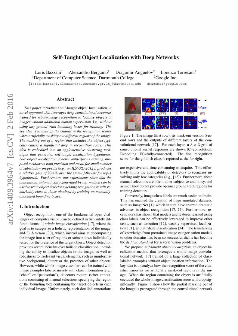
Figure 1: The image (first row), its mask-out version (sec-ond row) and the outputs of different layers of the con-volutional network [17]. For each layer, a 3 × 3 grid ofconvolutional kernel responses are shown (C=convolution,P=pooling, FC=fully-connected). The final recognitionscore for the goldfish class is reported at the far right.

are expensive and time-consuming to acquire. This effec-tively limits the applicability of detectors to scenarios in-volving only few categories (e.g., [12]). Furthermore, thesemanual selections are often rather subjective and noisy, andas such they do not provide optimal ground truth regions fortraining detectors.

Conversely, image class labels are much easier to obtain.This has enabled the creation of huge annotated datasets,such as ImageNet [1], which in turn have spurred dramaticadvances in object recognition [17, 27]. Furthermore, re-cent work has shown that models and features learned usingclass labels can be effectively leveraged to improve othertasks, such as detection [12], weakly-supervised localiza-tion [31], and attribute classification [34]. The transferringof knowledge from pretrained image categorization modelsto other domains has been so successful that it has becomethe de facto standard for several vision problems.

We propose self-taught object localization, an object lo-calization method that leverages a whole-image convolu-tional network [17] trained on a large collection of class-labeled examples without object location information. Thekey idea is to analyze how the recognition score of the clas-sifier varies as we artificially mask-out regions in the im-age. When the region containing the object is artificiallyoccluded the whole-image classification score will drop sig-nificantly. Figure 1 shows how the partial masking out ofthe image is propagated through the convolutional network

arX

iv:1

409.

3964

v7 [

cs.C

V]

2 F

eb 2

016

effecting the recognition score. This idea is embedded intoa hierarchical clustering technique similar to [30], whichmerges regions according to their relative drop in recogni-tion score. This produces for each image a set of subwin-dows that are deemed likely to contain the object.

The proposed method combines bottom-up groupingwith top-down (discriminative) information given by theconvolutional network. Moreover, we demonstrate that itcan be used in scenarios where the object label of the imageis not provided by analyzing the top-predicted classes.

The experiments on the ILSVRC-2012 dataset [1] showthat our method outperforms the state-of-the-art objectnessapproaches in terms of recall and precision when consid-ering a small budget of proposals. We obtained a relativeincrement of 23.4% in terms of top-1 recall with respect tothe state of the art. Moreover, a naive combination of ourapproach with proposal methods optimized for high recall,yields state-of-the-art results for any number of proposals inthe range from 1 to 104. We also show that our self-taughtlocalization model trained on the ILSVRC-2012 classes isable to generalize effectively to the different categories ofthe PASCAL 2007 dataset [8]. Finally, we demonstrate thatthe subwindows automatically-generated by our approachcan be used as positive training examples to learn objectdetectors without any additional human supervision. Ourdetection results on 200 classes of ILSVRC-2012 are closeto those obtained with the same detection model trained onmanually-annotated bounding boxes.

2. Related work

Several successful attempts have been made to applydeep networks to object localization and detection problems[12, 27, 29, 7]. In [12], a convolutional network [17] isfine-tuned on ground truth bounding boxes and then appliedto classify subwindows generated by selective search [30].In [27, 7, 29], the network is trained to perform regres-sion directly on the vector-space of bounding boxes. Thesedeep networks have shown promising results compared tostandard detection schemes relying on hand-crafted fea-tures (e.g., [10, 30]). However, all of these approaches re-quire manually-annotated bounding boxes as training data.In contrast, our method automatically populate the imageswith bounding boxes likely to contain object, which canthen be used for training detectors. We effectively replacethe traditional manually-selected bounding boxes with re-gions automatically estimated from training images anno-tated only with class labels, which are easy to obtain evenfor a large number of training images. This frameworkenables scalable training of object detectors at a much re-duced annotation cost. The idea of exploiting image classlabels for weakly-supervised localization was also exploredin [23]. In contrast, our method does not require to be re-trained or finetuned to generate object proposals.

Objectness methods [2, 6, 30, 4, 3, 16, 36, 25, 21, 26,32, 14] aim at generating bounding boxes that yield highrecall for a high number of candidates, i.e., they maximizethe probability that each object in the image is covered byat least one subwindow. These methods perform well attesting time and successfully replace the computationallyexpensive sliding window approach. However, they cannotbe used in lieu of ground truth bounding boxes to train adetector because of their low precision caused by the pres-ence of many false positives. Recently, convolutional net-works were used for region proposal [18, 24]. Howeverwe note that these methods require ground truth boundingboxes or regions during training and thus address a differ-ent task compared to ours. Our algorithm can be viewedas a class-specific subwindow proposal method which pro-vides precision superior to that of prior methods for lownumber of candidates. The precision of our approach ishigh enough that detectors trained on our automatically-generated bounding boxes perform nearly on par with de-tectors learned from ground-truth annotations. Moreover,during the training of detectors, the class label of each train-ing image is known. Our method exploits this informationto generate object-specific proposals which result in bettertraining of detectors compared to generic proposals.

Even though deep networks have shown impressive re-sults, there is still little understanding of what are the crit-ical factors contributing to their outstanding performance.In order to better comprehend deep networks, previouswork proposed to visualize the intermediate representations[33, 28], give semantic interpretation of individual units[19], study the emergence of detectors [35] or fool themwith artificial images [22]. Liu and Wang [20] have also an-alyzed what a classifier has learned but for the specific caseof bag of features and SVM. Instead, we study the effects ofselectively masking out the input of deep networks, whichcan provide new insights on what the network has learnedand how this can be exploited for object localization.

The idea of masking out the input of deep networks hasbeen explored in [33, 13, 5]. [33] investigates the corre-lation between occlusion of image regions and classifica-tion score for the purpose of visualizing the learned fea-tures. Although [33] did not provide quantitative resultson the task of localization, in our experiments we adaptedtheir occlusion-box strategy to perform object localizationbut we found that this yields much poorer results comparedto our approach (see Section 4 for details). The methodsin [13, 5] mask out the background to better focus on fore-ground features. Our idea is complementary, since we ex-ploit the foreground mask-out mechanism not simply as afeature analysis tool but also as an effective procedure toperform object localization. The method proposed in [28]computes a class-specific saliency maps by identifying thepixels that are most useful to predict the classification score

of a deep network. Instead, our approach provides state-of-the-art results even when used in a weakly-labeled setup.

3. Self-Taught object localizationThe aim of Self-Taught Localization (in brief STL) is to

generate bounding boxes that are very likely to contain ob-jects. The proposed approach relies on the idea of maskingout regions of an image provided as input to a deep network.The drop in recognition score caused by the masking out isembedded into an agglomerative clustering method whichmerges regions for object localization.

Input mask-out. Let us assume to have a deep networkf : RN 7→ RC that maps an image x ∈ RN of N pixelsto a confidence vector y ∈ RC of C classes. The confi-dence vector is defined as y = [y1, y2, . . . , yC ]

T , whereyi corresponds to the classification score of the i-th class.We propose to mask out the input image x by replacingthe pixel values in a given rectangular region of the im-age b = [bx, by, w, h] ∈ N4 with the 3-dimensional vec-tor g (one dimension for each image channel), where bxand by are the x and y coordinates and w and h are thewidth and height, respectively. The masking vector g islearned from a training set as the mean value of the indi-vidual image channels. We denote the function that masksout the image x given the region b using the vector g ashg : RN × N4 7→ RN . Please note that the output of thefunction is again an image (see Figure 1). The boundingboxes b are automatically generated by our agglomerativeclustering method (see details below).

We define the variation in classification score of the im-age x subject to the masking out of a bounding box b as theoutput value of function δf : RN × N4 7→ RC given by

δf (x,b) = max(f(x)− f(hg(x,b)),0) (1)

where the max and the difference operators are appliedcomponent-wise. This function compares the classificationscores of the original image to those of the masked-out im-age. Intuitively, if the difference for the c-th class is large,the masked-out region is very discriminative for that class.Thus the region b is likely to contain the object of class c.

We use the function δf to define two variants of drop inclassification score, depending on the availability of classlabel information for the image. When the ground truthclass label c of x is provided, we define the drop functiondCL : RN × N4 7→ R as

dCL(x,b) = δf (x,b)T Ic, (2)

where Ic ∈ NC is an indicator vector with 1 at the c-thposition and zeros elsewhere. This drop function enables usto generate class-specific proposals in order to populate atraining set with bounding boxes likely to contain instancesof class c. We denote the method which uses dCL as STLCL.

If the class information is not available, e.g. when test-ing a detector, we use the top-CI classes predicted by thewhole-image classifier f to define dWL : RN × N4 7→ R as

dWL(x,b) = δf (x,b)T Itop-CI

, (3)

where Itop-CI∈ NC is an indicator vector with ones at the

top-CI predictions for the image x and zeros elsewhere.Since the function relies on estimated class labels, the setupis called STLWL where WL stays for weakly labeled. In ourexperiments, we used the top-5 predictions of the deep net-work f applied to the whole image by leveraging the highrecognition accuracy of [17] (the probability of getting thecorrect class in the top-5 is 82%).

As deep convolutional network f we adopt the modelintroduced in [17] which has been proven to be very effec-tive for image classification. Since the network is appliedto mean-centered data, replacing a region of the image withthe learned mean RGB value is effectively equivalent to ze-roing out that section of the network input as well as thecorresponding units in the hidden convolutional layers (seeFigure 1). We want to point out that our masking-out ap-proach is general and it can be applied to any other classifierthat operates on raw pixels.

Agglomerative clustering. The proposed agglomerativeclustering approach is similar to that described in [30].Specifically, as in [30], we also employ the segmentationmethod proposed in [11] to generate the initial set ofK rect-angular1 regions {b1,b2, . . .bK}. Then the goal is to fuseregions (bottom-up) and generate windows that are likely tocontain objects (top-down). The main difference with re-spect to [30] is in the choice of the similarity used to fuseregions.

We propose an iterative method that greedily comparesthe available regions, and at each iteration merges the tworegions that maximize the similarity function discussed be-low. This procedure terminates when only one region (cov-ering the whole image) is left. The set of generated subwin-dows are then sorted according to the drop in classification(Eq. 2 for STLCL and Eq. 3 for STLWL). We also performnon-maximum suppression of the subwindows with overlapgreater than 50%.

We define the similarity between regions using fourterms capturing the intuitions expressed below. Two bound-ing boxes are likely to contain parts of the same object if

1. they cause similar large drops in classification score:

sdrop(x,bi,bj) =1− |dm(x,bi)− dm(x,bj)|·max (1− dm(x,bi), 1− dm(x,bj))

1Note that we mask out the bounding boxes enclosing the segmentsrather than the segments themselves. We found experimentally that if wemask out the segments, the shape information of the segment is preservedand used by the network to perform recognition, thus causing less substan-tial drops in classification.

2. they are similar in appearance:

sapp(x,bi,bj) = z(φ(x,bi), φ(x,bj))

3. they cover the image as much as possible, encouragingsmall windows to merge early (as in [30]):

ssize(x,bi,bj) = 1− size(bi) + size(bj)

size(x)

4. they are spatially near each other (as in [30]):

sfill(x,bi,bj) = 1− size(bi ∪ bj)− size(bi)− size(bj)

size(x)

where the index m ∈ {CL,WL} in the first term selectsSTLCL or STLWL presented in the previous subsection,z(·, ·) is the histogram intersection similarity between thenetwork features extracted by φ(·, ·) (see Sec. 4 for details),bi ∪ bj is the bounding box that contains bi and bj . Theoverall similarity score s is defined as a convex combinationof the terms above:

s(bi,bj ,x) =∑

l∈Lαl sl(bi,bj ,x), (4)

where L = {drop, app, size,fill} and the αs are set to beuniform weights in our experiments. We empirically foundthat removing sdrop from Eq. 4 will cause a drop of 8% and10% in terms of precision and recall, respectively.

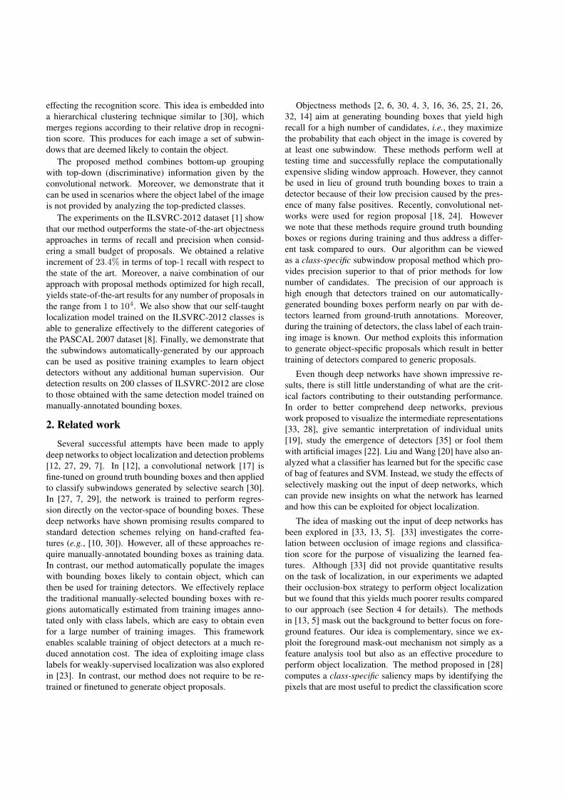
Figure 2 illustrates the intuition behind the similaritymeasure encoded by sdrop. This similarity is large if the tworegions exhibit similar classification drops when occluded(corresponding to points on the diagonal of the xy-plane inthe 3D plot) and it is especially large when the drop in scoreis substantial (points close to (1, 1) in the plot). The termsapp encourages aggregation of regions similar in appear-ance, while ssize and sfill borrowed from [30] favor earlymerging of small regions and regions that are near eachother, respectively.

There are many advantages of the proposed similaritywith respect to [30]. First, it does not rely on the hand-engineered features used in [30], but instead it leveragesthe features learned by the deep network. Moreover, oursimilarity exploits the discriminant power of the deep con-volutional network enabling our method to generate class-specific window proposals. Even when used in the weakly-labeled regime of Eq. 3 it will tend to generate subwindowsthat are most informative for recognition (since their occlu-sion causes large classification drops). Thus, our approachcan be viewed as a hybrid scheme combining bottom-upcues (size, appearance) with top-down information (object-class recognition), unlike [30] where the merging of regionsis driven by a pure bottom-up procedure.

Figure 2: Similarity score sdrop(·) as a function of the dropsin classification dk(x,bi) and dk(x,bj).

4. ExperimentsIn this section we present comparative results of our ap-

proach with state-of-the-art methods on the task of objectsubwindow proposal. We also show that STLCL can be usedto generate annotations for training object detectors.

Implementation details. In our experiments, we used theconvolutional network software Caffe [15] with the modeltrained on ILSVRC-2012 provided by the authors. Inspiredby [12], the descriptor (φ) used in the term sapp of STL isthe vector from the last fully-connected layer (before thesoft-max) of the network.

Datasets. Our experiments were carried out on twochallenging benchmarks: ILSVRC-2012-LOC [1] andPASCAL-VOC-2007 [8]. ILSVRC-2012-LOC is a large-scale benchmark for object localization containing 1000categories. The training set contains 544546 images with619207 annotated bounding boxes. The validation set con-tains 50000 images for a total of 76750 annotated boundingboxes. PASCAL-VOC-2007 contains 20 categories, for atotal of 9963 images divided into training, validation andtesting splits. Each image contains multiple objects belong-ing to different categories at different positions and scales,for a total of 24640 ground truth bounding boxes.

Object proposal. Given a test image, the goal is to gen-erate the best set of bounding boxes that enclose the objectsof interest with high probability. A true positive is a pro-posed bounding box whose intersection over union with theground truth is at least 50% [8]. The performance is thenmeasured in terms of the mean of the average recall and pre-cision per class [30] as done in the PASCAL benchmark [8].

We compared STL to recent state-of-the-art proposalmethods: SELSEARCH [30] (fast version), BING [4](MAXBGR version), EDGEBOXES [36] and MCG [3]. Wenote that these prior proposal methods do not make use ofimage class label when proposing subwindows. Thus, thesupervised version of STL (STLCL) is in a sense given anunfair advantage over them as it can generate class-specificproposals consistent with the ground-truth label. However,we will demonstrate that our weakly-labeled STLWL pro-vides results nearly equivalent to STLCL.

(a) ILSVRC-2012-LOC validation (b) PASCAL-VOC-2007 test

100

101

102

103

104

0.1

0.2

0.3

0.4

0.5

0.6

0.7

0.8

0.9

1

number of bboxes per image

me

an

re

ca

ll p

er

cla

ss

Selective Search [30]

BING [4]

EdgeBoxes [36]

MCG [3]

STL−CL (our method)

STL−WL (our method)

STL−WL+MCG

100

101

102

103

104

0.1

0.2

0.3

0.4

0.5

0.6

0.7

0.8

0.9

1

number of bboxes per image

me

an

re

ca

ll p

er

cla

ss

Selective Search [30]

BING [4]

EdgeBoxes [36]

MCG [3]

STL−WL (our method)

STL−WL+EdgeBoxes

100

101

102

103

104

0

0.1

0.2

0.3

0.4

0.5

0.6

0.7

number of bboxes per image

me

an

pre

cis

ion

pe

r cla

ss

Selective Search [30]

BING [4]

EdgeBoxes [36]

MCG [3]

STL−CL (our method)

STL−WL (our method)

STL−WL+MCG

100

101

102

103

104

0

0.05

0.1

0.15

0.2

0.25

0.3

0.35

number of bboxes per image

mean p

recis

ion p

er

cla

ss

Selective Search [30]

BING [4]

EdgeBoxes [36]

MCG [3]

STL−WL (our method)

STL−WL+EdgeBoxes

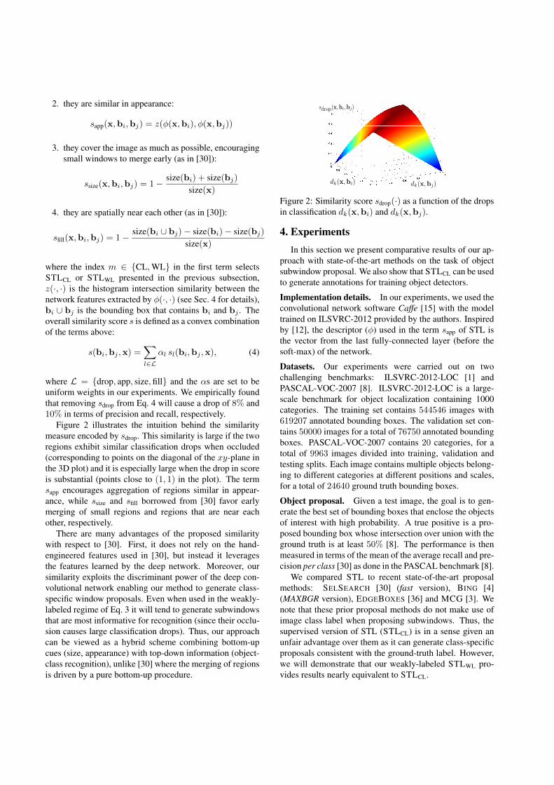
Figure 3: Comparison of different bounding-box proposal methods. The first and second row report the mean recall per classand the mean precision per class, respectively, as a function of the number of proposed subwindows. The columns show twodatasets: ILSVRC-2012-LOC (validation) and PASCAL-VOC-2007 (test).

Figure 3(a) reports the results in terms of recall (firstrow) and precision (second row) on the validation set ofILSVRC-2012-LOC. Note that this dataset is disjoint fromthe set used to train the convolutional network f . Fig-ure 3(a) shows that our method outperforms all the othermethods for the first 10 proposed subwindows. We obtaineda relative improvement in the top-1 recall of 23.4% overBING, which is the best method for the top-1 case. Fig-ure 3(a) also shows that the performance difference betweenusing the class label of the image (STLCL) and not usingit (STLWL) is negligible. This indicates that STL worksequally well even when the class label is not given.

SELSEARCH, BING, EDGEBOXES and MCG were de-signed to obtain high recall when using a large number ofproposals, which is a desirable property at testing time.However it yields precision not sufficiently high to traina detector as shown in Figures 3(a), second row. In con-trast, STL is by far the best method in term of both preci-sion and recall for a small number of proposals. In orderto capture the diversity between these methods, we carriedout an experiment where the top-10 proposals of STLWLare merged with the ones of the best performing methodfor large number of proposals, that is MCG. This experi-ment is reported in Figures 3(a) denoted as STLWL +MCG.This result demonstrates that we can obtain the best perfor-mance on the range 1-10 (where STLWL stands out) as wellas competitive results on the range 11-104 (where MCG isthe best) in terms of both recall and precision.

0.75 0.80 0.85 0.90 0.95 1.00Correlat ion

0.0

0.1

0.2

0.3

0.4

0.5

Top

-1re

ca

ll

aeroplane - wing

bicycle - bicycle-built -for-two

bird - hornbill

boat - dock

bot t le - restaurant

bus - t rolleybus

car - sports car

cat - Egypt ian cat

chair - restaurant

cow - ox

diningtable - restaurant

dog - Great Dane

horse - oxm otorbike - m otor scooter

person - st retcher

pot tedplant - pat io

sheep - ram

sofa - studio couch

t rain - steam locom ot ive

tvm onitor - m onitor

Max

Figure 4: Cross-dataset generalization. Each dot representsa PASCAL class: the x coordinate is its max correlationvalue against ILSVRC categories, while the y coordinateshows the top-1 recall achieved by STL on that PASCALcategory. The text for each dot lists the PASCAL class andits most correlated category in ILSVRC.

We also tested two simple baselines: the sliding win-dow and the sliding occlusion box. In the sliding windowapproach, a set of rectangles of different sizes is slid overthe image and at each position we compute the confidence

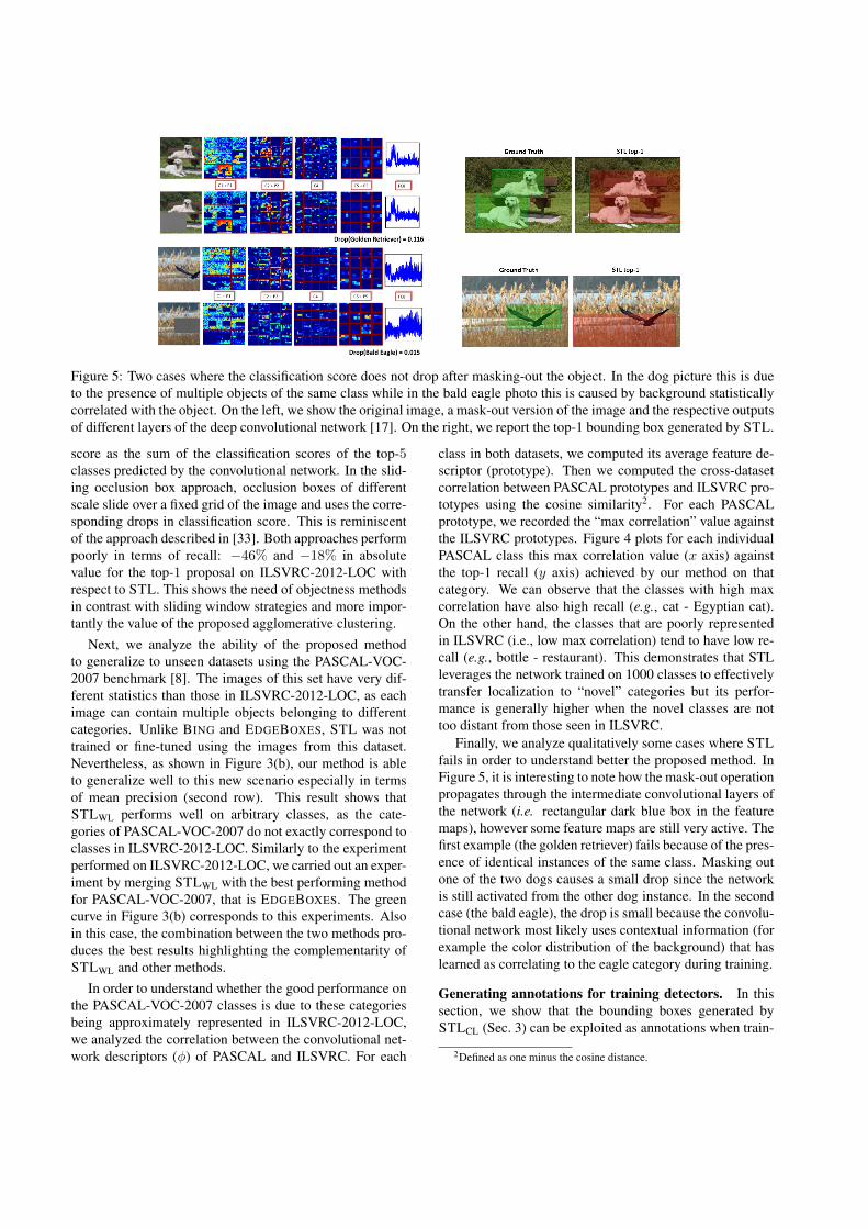
Figure 5: Two cases where the classification score does not drop after masking-out the object. In the dog picture this is dueto the presence of multiple objects of the same class while in the bald eagle photo this is caused by background statisticallycorrelated with the object. On the left, we show the original image, a mask-out version of the image and the respective outputsof different layers of the deep convolutional network [17]. On the right, we report the top-1 bounding box generated by STL.

score as the sum of the classification scores of the top-5classes predicted by the convolutional network. In the slid-ing occlusion box approach, occlusion boxes of differentscale slide over a fixed grid of the image and uses the corre-sponding drops in classification score. This is reminiscentof the approach described in [33]. Both approaches performpoorly in terms of recall: −46% and −18% in absolutevalue for the top-1 proposal on ILSVRC-2012-LOC withrespect to STL. This shows the need of objectness methodsin contrast with sliding window strategies and more impor-tantly the value of the proposed agglomerative clustering.

Next, we analyze the ability of the proposed methodto generalize to unseen datasets using the PASCAL-VOC-2007 benchmark [8]. The images of this set have very dif-ferent statistics than those in ILSVRC-2012-LOC, as eachimage can contain multiple objects belonging to differentcategories. Unlike BING and EDGEBOXES, STL was nottrained or fine-tuned using the images from this dataset.Nevertheless, as shown in Figure 3(b), our method is ableto generalize well to this new scenario especially in termsof mean precision (second row). This result shows thatSTLWL performs well on arbitrary classes, as the cate-gories of PASCAL-VOC-2007 do not exactly correspond toclasses in ILSVRC-2012-LOC. Similarly to the experimentperformed on ILSVRC-2012-LOC, we carried out an exper-iment by merging STLWL with the best performing methodfor PASCAL-VOC-2007, that is EDGEBOXES. The greencurve in Figure 3(b) corresponds to this experiments. Alsoin this case, the combination between the two methods pro-duces the best results highlighting the complementarity ofSTLWL and other methods.

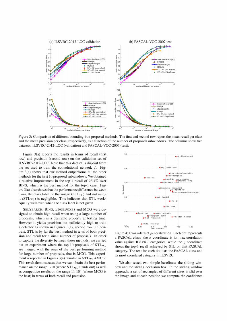
In order to understand whether the good performance onthe PASCAL-VOC-2007 classes is due to these categoriesbeing approximately represented in ILSVRC-2012-LOC,we analyzed the correlation between the convolutional net-work descriptors (φ) of PASCAL and ILSVRC. For each

class in both datasets, we computed its average feature de-scriptor (prototype). Then we computed the cross-datasetcorrelation between PASCAL prototypes and ILSVRC pro-totypes using the cosine similarity2. For each PASCALprototype, we recorded the “max correlation” value againstthe ILSVRC prototypes. Figure 4 plots for each individualPASCAL class this max correlation value (x axis) againstthe top-1 recall (y axis) achieved by our method on thatcategory. We can observe that the classes with high maxcorrelation have also high recall (e.g., cat - Egyptian cat).On the other hand, the classes that are poorly representedin ILSVRC (i.e., low max correlation) tend to have low re-call (e.g., bottle - restaurant). This demonstrates that STLleverages the network trained on 1000 classes to effectivelytransfer localization to “novel” categories but its perfor-mance is generally higher when the novel classes are nottoo distant from those seen in ILSVRC.

Finally, we analyze qualitatively some cases where STLfails in order to understand better the proposed method. InFigure 5, it is interesting to note how the mask-out operationpropagates through the intermediate convolutional layers ofthe network (i.e. rectangular dark blue box in the featuremaps), however some feature maps are still very active. Thefirst example (the golden retriever) fails because of the pres-ence of identical instances of the same class. Masking outone of the two dogs causes a small drop since the networkis still activated from the other dog instance. In the secondcase (the bald eagle), the drop is small because the convolu-tional network most likely uses contextual information (forexample the color distribution of the background) that haslearned as correlating to the eagle category during training.

Generating annotations for training detectors. In thissection, we show that the bounding boxes generated bySTLCL (Sec. 3) can be exploited as annotations when train-

2Defined as one minus the cosine distance.

Positive Boxes + BING [4] + EDGEBOXES [36] + MCG [3] + SELSEARCH [30] + STLCL (our) + GROUNDTRUTH +Negative/Test Boxes BING EDGEBOXES MCG SELSEARCH STLWL (our) SELSEARCH

mAP 13.78 17.03 17.94 18.31 19.60 25.40

Table 1: The first row reports which method is used to generate the bounding boxes of the positive set, and those of thenegative and test set. The second row contains the mean Average Precision (%) calculated as the mean across all 200 classesfor ILSVRC-2012-LOC-200.

Positive Boxes + BING [4] + SELSEARCH [30] + STLCL (our method) + GROUNDTRUTH +Negative/Test Boxes SELSEARCH SELSEARCH SELSEARCH SELSEARCH

mAP (all classes) 19.55 18.31 20.43 25.40leopard = 56.83 leopard = 59.29 leopard = 62.86 leopard = 65.28giant panda = 50.73 car mirror = 50.86 teapot = 57.26 Crock Pot = 62.60koala = 49.50 koala = 49.23 giant panda = 54.96 teapot = 59.12car mirror = 48.25 admiral = 44.96 car mirror = 51.69 admiral = 58.55

best classes orangutan = 46.76 giant panda = 44.19 Crock Pot = 50.56 car mirror = 58.28pickup = 45.09 crib = 41.21 koala = 50.15 koala = 55.63admiral = 44.69 bullfrog = 41.00 police van = 48.37 cabbage butterfly = 54.73frilled lizard = 44.57 maze = 40.67 admiral = 46.24 frilled lizard = 52.10entertainment center = 43.04 orangutan = 40.66 necklace = 46.05 police van = 51.86teapot = 42.67 whiskey jug = 38.27 pickup = 45.75 giant panda = 51.68flute = 0.21 punching bag = 0.12 croquet ball = 0.15 punching bag = 0.63punching bag = 0.21 hair spray = 0.03 punching bag = 0.13 hair spray = 0.54

worst classes swimming trunks = 0.16 basketball = 0.01 basketball = 0.11 screwdriver = 0.41pole = 0.03 pole = 0.01 pole = 0.10 nail = 0.10basketball = 0.01 nail = 0.01 nail = 0.04 pole = 0.05

Table 2: Each column contains the best classes (blue) and the worst classes (red) for the detectors trained using the annotationmethod listed at the top, along with the Average Precision (%). All methods were trained on ILSVRC-2012-LOC-200.

ing object detectors, thus eliminating the need for groundtruth annotations. To this end, we use a subset of 200 ran-domly selected classes from ILSVRC-2012-LOC (whichwe denote as ILSVRC-2012-LOC-2003) as this allowed usto perform faster training, thus enabling a more comprehen-sive study of the different methods on the detection task.

200 detectors were trained (one for each class inILSVRC-2012-LOC-200), using for each a training set of50 positive images and 4975 negative images (obtained bysampling 25 examples from each negative class). The testset is composed by 10000 images of the ILSVRC-2012-LOC-200 validation set. As detection model, we use theRCNN detector of [12], with the difference that we trainit with the simpler negative mining procedure describedin [30]. However, while [30, 12] exploited manually-annotated bounding boxes as positive examples, in ourtraining procedure we replace the ground truth regions withthe top-K bounding boxes produced by the class-specificSTLCL on training images of class c, i.e., we use the classlabel information for localization of the positive regions.

The negative set is built using the bounding boxes thatoverlap less than 30% with any STLCL subwindows fromthe positive images, and one randomly-chosen boundingbox from each negative image. At each iteration, a linearSVM [9] is trained by automatically choosing the hyper-parameter with a 5-fold cross-validation that maximizes theaverage precision. The negative set is augmented for thenext training iteration by adding for each negative imagethe bounding box with the highest positive score.At testing

3To enable future comparisons with our results, we will make publiclyavailable the list of 200 classes.

time, each detector is tested on the generated subwindowsof a given image, the detection scores are sorted and thenpruned via non-maximum suppression: we remove a sub-window if it overlaps for more than 70% with a subwindowthat has higher score.

We experimented with different combinations of pro-posal methods for the positive and the negative boundingboxes. For each combination, at test time on each input im-age we used the same proposal method that was applied togenerate the negative boxes during training. For all com-binations we use the top-3 candidates as positive boundingboxes to obtain a good recall/precision trade-off based onthe results of Figure 3.

Table 1 shows the results in terms of mean average preci-sion (mAP) across all the 200 classes for each method com-puted according to the PASCAL VOC criterion [8]. Thefirst row reports the method used to generate the positivetraining boxes, the second row indicated the method for thenegative and test boxes. Our approach is STLCL+STLWL(sixth column of Table 1), and it involves using our proposalmethod based on class labels (since when training a detectorthey are always available) to generate the positive boxes andour unsupervised approach to produce the negative boxes aswell as the proposals on the test images. We compare thisapproach to BING, EDGEBOXES, MCG and SELSEARCH,where each of these methods was used to generate both thepositive boxes as well as the negative and testing boxesof the detector (second to fifth columns of Table 1). Wealso compared our method to the fully-supervised approachbased on manually-annotated positive boxes as proposedin [30] (named GROUNDTRUTH+SELSEARCH in Table 1).

0 0.2 0.4 0.60

0.1

0.2

0.3

0.4

0.5

0.6

AP − Ground truth+SelSearch

AP

− S

TL

−C

L+

Se

lSe

arc

h

Figure 6: Average precision (AP) on the individual200 classes obtained with the fully-supervised approachGROUNDTRUTH+SELSEARCH (x-axis) and our methodSTLCL+SELSEARCH (y-axis). Each point represents theAP of these two methods on one particular class.

We notice that STLCL+STLWL outperforms all the othermethods, yielding a relative improvement of 42.2% overthe worse method (BING) and 7% over the best competitor(SELSEARCH). This suggests that STLCL generates reli-able bounding boxes for the positive set.

An interesting observation that can be drawn from Fig-ure 3(a) is that while STLCL produces the highest preci-sion for a small number of subwindows (and therefore it isthe preferred method to generate the positive boxes), othermethods yield higher recall for large numbers of proposals.This suggests that using, for example, SELSEARCH for thenegative and test images can be advantageous. Based on thisobservation, we performed an experiment where we tested“the best of the two worlds”, i.e., using STLCL to generatethe positive set and SELSEARCH for the negative and testset (Table 2, fourth column). We also tested combinationof other proposal methods for positive subwindows withSELSEARCH for negative/test subwindows and reported theresults on Table 2 (second and third column). Table 2 (sec-ond row) shows that STLCL+SELSEARCH outperforms allthe other combinations. Moreover, STLCL+SELSEARCHshows a relative drop in performance of only 19.6% withrespect to the fully supervised method (last column). Thisis a remarkable result given that it uses only class labels. Wealso tested STLCL+SELSEARCH using the top-1 boundingbox obtaining a mAP of 20.93%, which reduces to 17.6%the relative gap with respect to the fully-supervised method.

Table 2 shows also the best-10 and worst-5 classes foreach method along with the respective APs. It is interestingto notice that 8 out of the 10 best categories are shared be-tween the detectors trained on the ground truth annotations(last column) and our STLCL (forth column) as opposed to5 out of 10 of our competitors.

In Figure 6 we report the AP on each individual class forthe proposed method STLCL+SELSEARCH (y-axis) and thefully-supervised approach GROUNDTRUTH+SELSEARCH

(x-axis). For 41 classes (all points above the diagonal)the proposed method achieves better accuracy than that ob-tained when using ground truth annotations.

Analysis of computational costs. Let K be the numberof segments produced by the method of [11]. During initial-ization, the similarity of Eq. 4 is evaluated for all segmentpairs, for a total of O(K2) times. However, note that onlyK evaluations of the convolutional network are needed, onefor each masked-out segment (Eq. 1).

At the first iteration of the clustering procedure, two ofthe segments are merged, and there will be K − 1 remain-ing segments. Only the similarities involving the newly cre-ated segment are updated, which amount to O(K) similarityevaluations, but these can be obtained with a single networkevaluation of the image with only the newly merged seg-ment masked-out. In every subsequent iteration, the totalnumber of segments will decrease by one. Thus, in totalonly 2 ·K network evaluations are performed over the en-tire procedure, including those done at initialization.

In practice, the 2 · K network evaluations of an imagetake about 210 seconds on CPU or 20 seconds on GPU fortypical values of K using our non-optimized Python code.MCG, EDGEBOXES, SELSEARCH and BING are highlyoptimized and they take 25, 0.25, 10 and 0.2 seconds perimage, respectively. The runtime of STL can be optimizedby merging only adjacent segments during agglomerativeclustering. Note that most of the computation is done duringthe initialization of the clustering algorithm (whenK mask-out operations are performed). At the same time, these seg-ments are very small and therefore most of the ConvNet fea-tures with limited receptive field do not change. We leavethe optimization of the STL code as future work.

5. ConclusionsThis work presents self-taught localization, which lever-

ages the power of convolutional networks trained using im-age class labels to automatically object proposal subwin-dows. We showed that STL outperforms the state-of-the-art methods on the task of object localization. We demon-strated that detectors trained on localization hypotheses au-tomatically generated by STL achieve performance nearlycomparable to those produced when training on manuallyselected bounding boxes. In future work we will investi-gate the possibility of fine-tuning the network as a localizeron the subwindows generated by STL and how to use themin a multiple instance learning framework in order to havemore robust object detectors. The code of our method willbe made publicly available.

Acknowledgements. We thank Haris Baig for helpfuldiscussion. This work was funded in part by Google, NSFaward CNS-1205521 and a CompX Faculty Grant from theWilliam H. Neukom 1964 Institute for Computational Sci-ence.

References[1] Large scale visual recognition challenge, 2012.

http://www.image-net.org/challenges/LSVRC/2012/.

[2] B. Alexe, T. Deselaers, and V. Ferrari. Measuring the object-ness of image windows. Pattern Analysis and Machine In-telligence, IEEE Transactions on, 34(11):2189–2202, 2012.

[3] P. Arbelaez, J. Pont-Tuset, J. T. Barron, F. Marques, andJ. Malik. Multiscale combinatorial grouping. In IEEE CVPR,2014.

[4] M. Cheng, Z. Zhang, W. Lin, and P. Torr. Bing: Binarizednormed gradients for objectness estimation at 300fps. InIEEE CVPR, 2014.

[5] J. Dai, K. He, and J. Sun. Convolutional feature masking forjoint object and stuff segmentation. In IEEE CVPR, 2015.

[6] I. Endres and D. Hoiem. Category-independent object pro-posals with diverse ranking. Pattern Analysis and MachineIntelligence, IEEE Transactions on, 36(2), 2014.

[7] D. Erhan, C. Szegedy, A. Toshev, and D. Anguelov. Scalableobject detection using deep neural networks. In IEEE CVPR,2014.

[8] M. Everingham, L. Van Gool, C. K. I. Williams, J. Winn,and A. Zisserman. The PASCAL Visual Object ClassesChallenge 2007 (VOC2007) Results. http://www.pascal-network.org/challenges/VOC/voc2007/workshop/index.html.

[9] R. Fan, K. Chang, C. Hsieh, X. Wang, and C. Lin. Liblinear:A library for large linear classification. JMLR, 9, 2008.

[10] P. F. Felzenszwalb, R. B. Girshick, D. McAllester, and D. Ra-manan. Object detection with discriminatively trained part-based models. Pattern Analysis and Machine Intelligence,IEEE Transactions on, 32(9):1627–1645, 2010.

[11] P. F. Felzenszwalb and D. P. Huttenlocher. Efficientgraph-based image segmentation. Int. J. Comput. Vision,59(2):167–181, September 2004.

[12] R. Girshick, J. Donahue, T. Darrell, and J. Malik. Rich fea-ture hierarchies for accurate object detection and semanticsegmentation. In IEEE CVPR, 2014.

[13] B. Hariharan, P. Arbelaez, B. Girshick, and J. Malik. Simul-taneous detection and segmentation. In ECCV, 2014.

[14] J. Hosang, R. Benenson, and B. Schiele. How good are de-tection proposals, really? In BMVC, 2014.

[15] Y. Jia, E. Shelhamer, J. Donahue, S. Karayev, J. Long, R. Gir-shick, S. Guadarrama, and T. Darrell. Caffe: Convolu-tional architecture for fast feature embedding. arXiv preprintarXiv:1408.5093, 2014.

[16] P. Krahenbuhl and V. Koltun. Geodesic object proposals. InECCV 2014, pages 725–739. 2014.

[17] A. Krizhevsky, I. Sutskever, and G. E. Hinton. Imagenetclassification with deep convolutional neural networks. InNIPS, pages 1097–1105. 2012.

[18] W. Kuo, B. Hariharan, and J. Malik. Deepbox:learning ob-jectness with convolutional networks. In ICCV, 2015.

[19] Q. Le, M. Ranzato, R. Monga, M. Devin, K. Chen, G. Cor-rado, J. Dean, and A. Ng. Building high-level features usinglarge scale unsupervised learning. In ICML, 2012.

[20] L. Liu and L. Wang. What has my classifier learned? vi-sualizing the classification rules of bag-of-feature model bysupport region detection. In IEEE CVPR, 2012.

[21] S. Manen, M. Guillaumin, and L. Van Gool. Prime objectproposals with randomized prim’s algorithm. In IEEE ICCV,pages 2536–2543. IEEE, 2013.

[22] A. Nguyen, J. Yosinski, and J. Clune. Deep neural networksare easily fooled: High confidence predictions for unrecog-nizable images. In IEEE CVPR, 2015.

[23] M. Oquab, L. Bottou, I. Laptev, and J. Sivic. Is object local-ization for free? - weakly-supervised learning with convolu-tional neural networks. In IEEE CVPR, 2015.

[24] P. O. Pinheiro, R. Collobert, and P. Dollar. Learning to seg-ment object candidates. In NIPS, 2015.

[25] E. Rahtu, J. Kannala, and M. Blaschko. Learning a categoryindependent object detection cascade. In IEEE ICCV, pages1052–1059, 2011.

[26] P. Rantalankila, J. Kannala, and E. Rahtu. Generating ob-ject segmentation proposals using global and local search. InIEEE CVPR, pages 2417–2424. IEEE, 2014.

[27] P. Sermanet, D. Eigen, X. Zhang, M. Mathieu, R. Fergus,and Y. LeCun. Overfeat: Integrated recognition, localizationand detection using convolutional networks. In ICLR, 2014.

[28] K. Simonyan, A. Vedaldi, and A. Zisserman. Deep in-side convolutional networks: Visualising image classifica-tion models and saliency maps. In ICLR Workshop, 2014.

[29] C. Szegedy, A. Toshev, and D. Erhan. Deep neural networksfor object detection. In NIPS, pages 2553–2561, 2013.

[30] J. R. R. Uijlings, K. E. A. van de Sande, T. Gevers, andA. W. M. Smeulders. Selective search for object recognition.Int. J. Comput. Vision, 104(2):154–171, 2013.

[31] C. Wang, W. Ren, K. Huang, and T. Tan. Weakly supervisedobject localization with latent category learning. In ECCV2014, pages 431–445, 2014.

[32] C. Wang, L. Zhao, S. Liang, L. Zhang, J. Jia, and Y. Wei.Object proposal by multi-branch hierarchical segmentation.In IEEE CVPR, 2015.

[33] M. D. Zeiler and R. Fergus. Visualizing and understandingconvolutional neural networks. In ECCV, 2014.

[34] N. Zhang, M. Paluri, M. Ranzato, T. Darrell, and L. Bourdev.Panda: Pose aligned networks for deep attribute modeling. InIEEE CVPR, pages 1637–1644, 2014.

[35] B. Zhou, A. Khosla, A. Lapedriza, A. Oliva, and A. Torralba.Object detectors emerge in deep scene cnns. In ICLR, 2015.

[36] C L. Zitnick and P. Dollar. Edge boxes: Locating objectproposals from edges. In ECCV 2014, pages 391–405. 2014.

Supplementary Material

Abstract

In this supplementary material we provide further ev-idence that supports the quality of the proposed method.These additional experiments were produced using the sameversion of the algorithm explained in our paper and in-clude:

• Visualization of the mask-out effect in terms of convo-lutional feature maps and drop in classification (Fig-ures 1 and 2);

• Visualization of top-1 bounding boxes generated bySTLCL (our method) and SELSEARCH [1] (Table 1).

Note: this document is best viewed in color.

Visualizing the Mask-out EffectWe show some qualitative examples of the effect of the

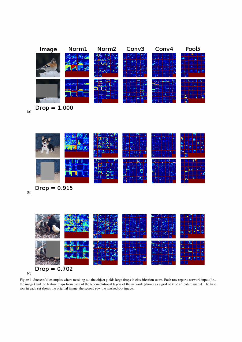
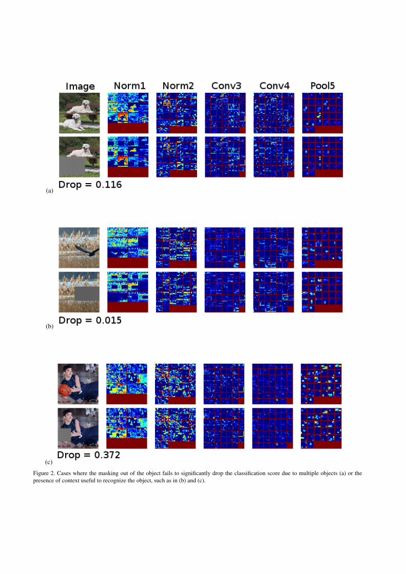
mask-out operation on images in Figure 1 and 2. Each rowreports network input (i.e., the image) and feature mapsfrom each of the 5 convolutional layers of the network(shown as a grid of F × F feature maps). The first rowin each set shows the original images, while the second rowshows the effects on the the masked-out image. We alsoreport the value of the drop in classification (Eq. 1 in thepaper) caused by to the mask-out operation.

In Fig. 1, we can see some cases where the proposedmethod succeeds, i.e., where masking out the object regioncauses a significant drop in classification score. It is inter-esting to visually note how the mask-out operation propa-gates through the intermediate convolutional layers of thenet until reaching the classification output (as evidenced bythe drop). The mask-out operation essentially correspondsto zeroing out the feature map values corresponding to pix-els in the masked-out region (e.g. rectangular dark blue boxin norm1 feature maps).

Fig. 2 shows some hard examples where our localizationmethod is prone to fail because the drop in recognition is nothigh. In Fig. 2(a), masking out one of the two dogs causes asmall drop since there is still one dog that can be recognizedby the network. Moreover, a small drop may happen alsowhen the convolutional network uses contextual informa-tion (for example the color distribution of the background)

that has learned as correlating to some specific category dur-ing training, e.g., the eagle and the background landscape inFig. 2(b). Finally, the basketball example in Fig. 2(c) showsthat the network is still able to classify the object (the ball)even when the object of interest is masked out. This is dueto the frequent co-occurrence in the training set of basket-ball and basketball player. The network therefore learnedthe co-occurrence of the two different objects but not thecharacteristic of the basketball itself. Fortunately, becauseSTL relies on three other terms it can propose good subwin-dows also in cases where the mask-out term fails.

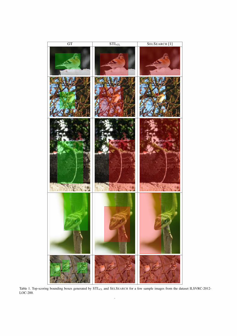
We show in Table 1 the top-scoring bounding box on afew sample images of the dataset ILSVRC-2012-LOC, us-ing different bounding box proposal methods. In the caseof our method (STLCL), we show the top bounding box se-lected according to Eq. 1 in the paper. As already high-lighted by the quantitative results, the subwindows pro-duced by STLCL are more accurate than those producedby SELSEARCH. It is also interesting to notice in the lastrow of the table that multiple similar instances of the sameobject are often grouped together because STLCL yieldsthe maximum drop in classification when all of them aremasked out.

References[1] J. R. R. Uijlings, K. E. A. van de Sande, T. Gevers, and

A. W. M. Smeulders. Selective search for object recognition.Int. J. Comput. Vision, 104(2):154–171, 2013.

1

(a)

(b)

(c)

Figure 1. Successful examples where masking out the object yields large drops in classification score. Each row reports network input (i.e.,the image) and the feature maps from each of the 5 convolutional layers of the network (shown as a grid of F × F feature maps). The firstrow in each set shows the original image, the second row the masked-out image.

(a)

(b)

(c)

Figure 2. Cases where the masking out of the object fails to significantly drop the classification score due to multiple objects (a) or thepresence of context useful to recognize the object, such as in (b) and (c).

GT STLCL SELSEARCH [1]

Table 1. Top-scoring bounding boxes generated by STLCL and SELSEARCH for a few sample images from the dataset ILSVRC-2012-LOC-200.

.