(sem) essentials structural equation...

1

Structural Equation Modeling (SEM) Essentials

byJim Grace

Purpose of this module is to provide a very brief presentation of the things one needs to know about SEM before learning how apply SEM.

2

Where You can Learn More about SEMGrace (2006) Structural Equation Modeling and Natural Systems.

Cambridge Univ. Press.

Shipley (2000) Cause and Correlation in Biology. Cambridge Univ. Press.

Kline (2005) Principles and Practice of Structural Equation Modeling. (2nd Edition) Guilford Press.

Bollen (1989) Structural Equations with Latent Variables. John Wiley and Sons.

Lee (2007) Structural Equation Modeling: A Bayesian Approach. John Wiley and Sons.

3

I. Essential Points about SEM

Outline

II. Structural Equation Models: Form and Function

4

I. SEM Essentials:

1. SEM is a form of graphical modeling, and therefore, a system in which relationships can be represented in either graphical or equational form.

x1 y1

ζ1γ11graphicalform

y1 = γ11x1 + ζ1equationalform

2. An equation is said to be structural if there exists sufficient evidence from all available sources to support the interpretation that x1 has a causal effect on y1.

5

y2y1

x1 y3

ζ1 ζ2

ζ3

Complex Hypothesis

e.g.y1 = γ11x1 + ζ1y2 = β 21y1 + γ 21x1 + ζ 2y3 = β 32y2 + γ31x1 + ζ 3

CorrespondingEquations

3. Structural equation modeling can be defined as the use of two or more structural equations to represent complex hypotheses.

6

a. manipulations of x can repeatably be demonstrated to be followed by responses in y, and/or

b. we can assume that the values of x that we have can serve as indicators for the values of x that existed when effects on y were being generated, and/or

c. if it can be assumed that a manipulation of x would result in a subsequent change in the values of y

Relevant References:

Pearl (2000) Causality. Cambridge University Press. Shipley (2000) Cause and Correlation in Biology. Cambridge

4. Some practical criteria for supporting an assumption of causal relationships in structural equations:

7

5. A Grossly Oversimplified History of SEM

Wright(1918)

Pearson(1890s) Fisher

(1922)

Joreskog(1973)

Lee(2007)

Neyman & E. Pearson(1934)

Spearman(1904)

Bayes & LaPlace(1773/1774)

MCMC(1948-)

test

ing

alt.

mod

els

likelih

ood

r, chi-square

factor analysis

path analysis SEM

Contemporary

Conven-tionalStatistics

BayesianAnalysisRaftery

(1993)

note that SEM is a framework and incorporates new statistical techniques as they become available (if appropriate to its purpose)

8

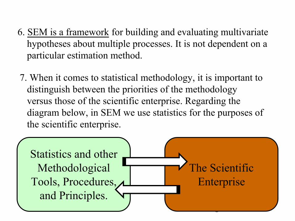
6. SEM is a framework for building and evaluating multivariate hypotheses about multiple processes. It is not dependent on a particular estimation method.

7. When it comes to statistical methodology, it is important to distinguish between the priorities of the methodology versus those of the scientific enterprise. Regarding the diagram below, in SEM we use statistics for the purposes of the scientific enterprise.

Statistics and other Methodological

Tools, Procedures, and Principles.

The Scientific Enterprise

9

The Methodological Side of SEM

10

The Relationship of SEM to the Scientific Enterprise

modified from Starfield and Bleloch (1991)

Understanding of Processes

univariatedescriptive statistics

exploration,methodology and

theory development

realisticpredictive models

simplisticmodels

multivariatedescriptive statistics

detailed processmodels

univariate datamodeling

Data

structuralequationmodeling

11

8. SEM seeks to progress knowledge through cumulative learning. Current work is striving to increase the capacity for model memory and model generality.

exploratory/model-building

applications

structural equation modeling

confirmatory/hypothesis-testing

applicationsone aim ofSEM

12

9. It is not widely understood that the univariate model, and especially ANOVA, is not well suited for studying systems, but rather, is designed for studying individual processes, net effects, or for identifying predictors.

10. The dominance of the univariate statistical model in the natural sciences has, in my personal view, retarded the progress of science.

13

11. An interest in systems under multivariate control motivates us to explicitly consider the relative importances of multiple processes and how they interact. We seek to consider simultaneously the main factors that determine how system responses behave.

12. SEM is one of the few applications of statistical inference where the results of estimation are frequently “you have the wrong model!”. This feedback comes from the unique feature that in SEM we compare patterns in the data to those implied by the model. This is an extremely important form of learning about systems.

14

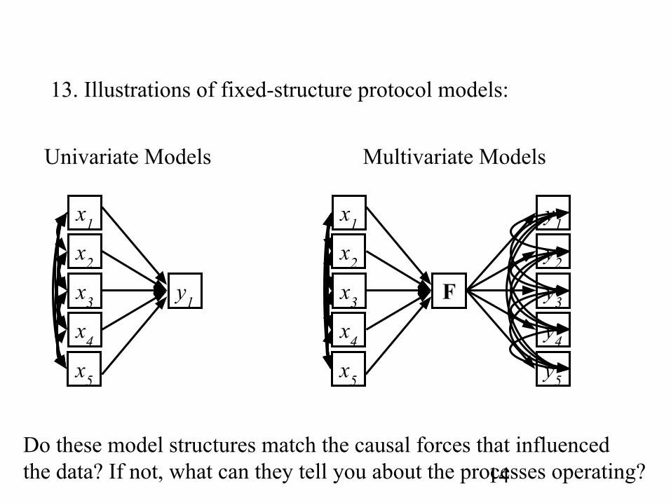
13. Illustrations of fixed-structure protocol models:

Univariate Models

x1

x2

x3

x4

x5

y1

Multivariate Models

x1

x2

x3

x4

x5

F

y1

y2

y3

y4

y5

Do these model structures match the causal forces that influencedthe data? If not, what can they tell you about the processes operating?

15

14. Structural equation modeling and its associated scientific goals represent an ambitious undertaking. We should be both humbled by the limits of our successes and inspired by the learning that takes place during the journey.

16


A. Anatomy of Observed Variable Models

17

x1

y1

y2

ζ1

ζ2

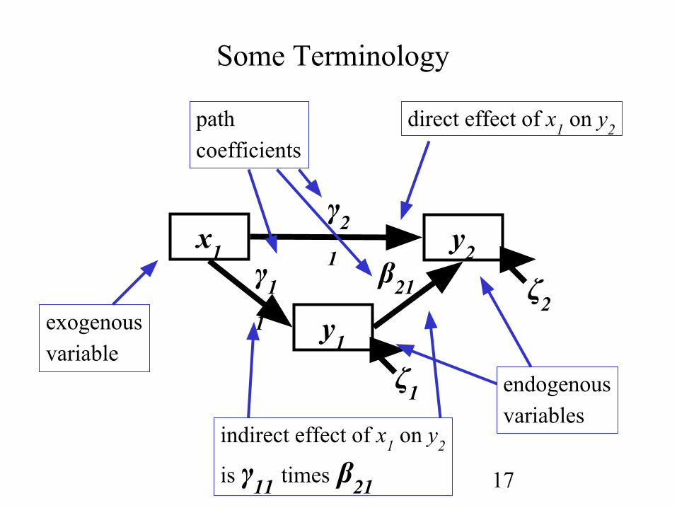
Some Terminology

exogenousvariable

endogenousvariables

γ2

1γ1

1

β21

path coefficients

direct effect of x1 on y2

indirect effect of x1 on y2

is γ11 times β21

18

nonrecursive

y1x2

x1 y2

ζ1

ζ2

C

y1x2

x1 y2

ζ1

ζ2

D

x1 y1

ζ1

y2

A

ζ2

x1 y1 y2

B

ζ1ζ2

model B, which has paths between all variables is “saturated” (vs A, which is “unsaturated”)

19

First Rule of Path Coefficients: the path coefficients forunanalyzed relationships (curved arrows) between exogenous variables are simply the correlations (standardized form) or covariances (unstandardized form).

x1

x2

y1.40

x1 x2 y1-----------------------------x1 1.0x2 0.40 1.0y1 0.50 0.60 1.0

20

x1 y1 y2

γ11 = .50 β21 = .60

γ (gamma) used to represent effect of exogenous on endogenous.β (beta) used to represent effect of endogenous on endogenous.

Second Rule of Path Coefficients: when variables areconnected by a single causal path, the pathcoefficient is simply the standardized or unstandardized regression coefficient (note that a standardized regression coefficient = a simple correlation.)

x1 y1 y2-------------------------------------------------x1 1.0y1 0.50 1.0y2 0.30 0.60 1.0

21

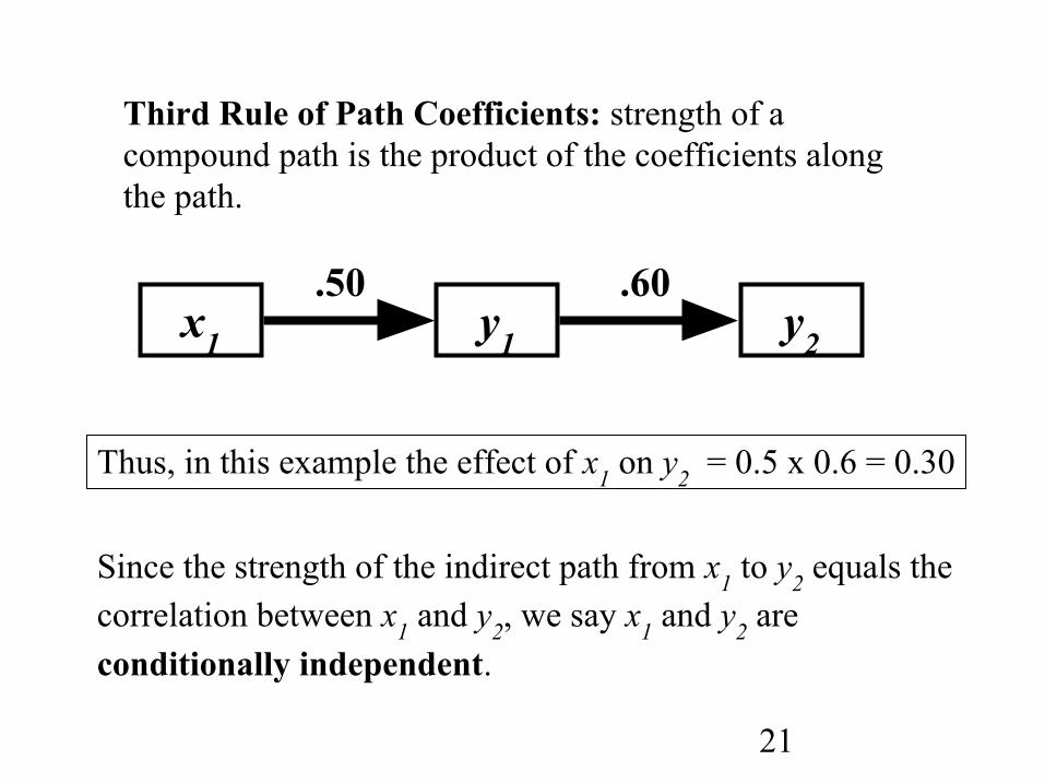
Third Rule of Path Coefficients: strength of a compound path is the product of the coefficients along the path.

x1 y1 y2

.50 .60

Thus, in this example the effect of x1 on y2 = 0.5 x 0.6 = 0.30

Since the strength of the indirect path from x1 to y2 equals the correlation between x1 and y2, we say x1 and y2 are conditionally independent.

22

What does it mean when two separated variables are not conditionally independent?

x1 y1 y2-------------------------------------------------x1 1.0y1 0.55 1.0y2 0.50 0.60 1.0

x1 y1 y2

r = .55 r = .60

0.55 x 0.60 = 0.33, which is not equal to 0.50

23

The inequality implies that the true model is

x1

y1

y2

Fourth Rule of Path Coefficients: when variables areconnected by more than one causal pathway, the path coefficients are "partial" regression coefficients.

additional process

Which pairs of variables are connected by two causal paths?

answer: x1 and y2 (obvious one), but also y1 and y2, which are connected by the joint influence of x1 on both of them.

24

And for another case:

x1

x2

y1

A case of shared causal influence: the unanalyzed relationbetween x1 and x2 represents the effects of an unspecifiedjoint causal process. Therefore, x1 and y1 connected by two causal paths. x2 and y1 likewise.

25

x1

y1

y2

.40

.31

.48

How to Interpret Partial Path Coefficients: - The Concept of Statistical Control

The effect of y1 on y2 is controlled for the joint effects of x1.

I have an article on this subject that is brief and to the point.Grace, J.B. and K.A. Bollen 2005. Interpreting the results from multiple

regression and structural equation models. Bull. Ecological Soc. Amer. 86:283-295.

26

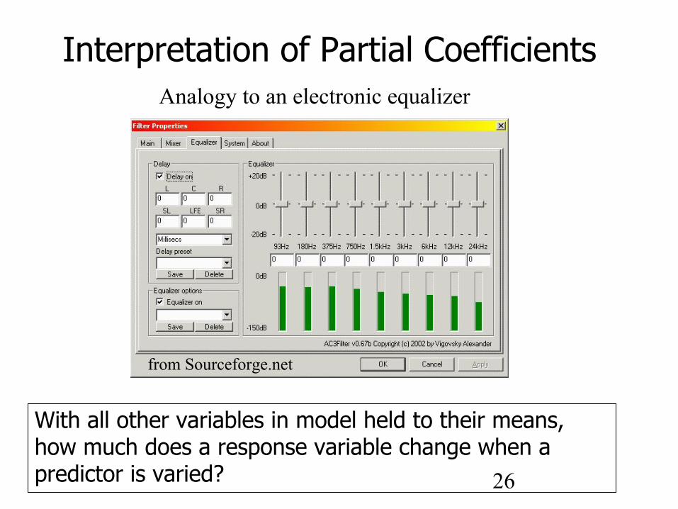
Interpretation of Partial CoefficientsAnalogy to an electronic equalizer

from Sourceforge.net

With all other variables in model held to their means, how much does a response variable change when a predictor is varied?

27

x1

y1

y2

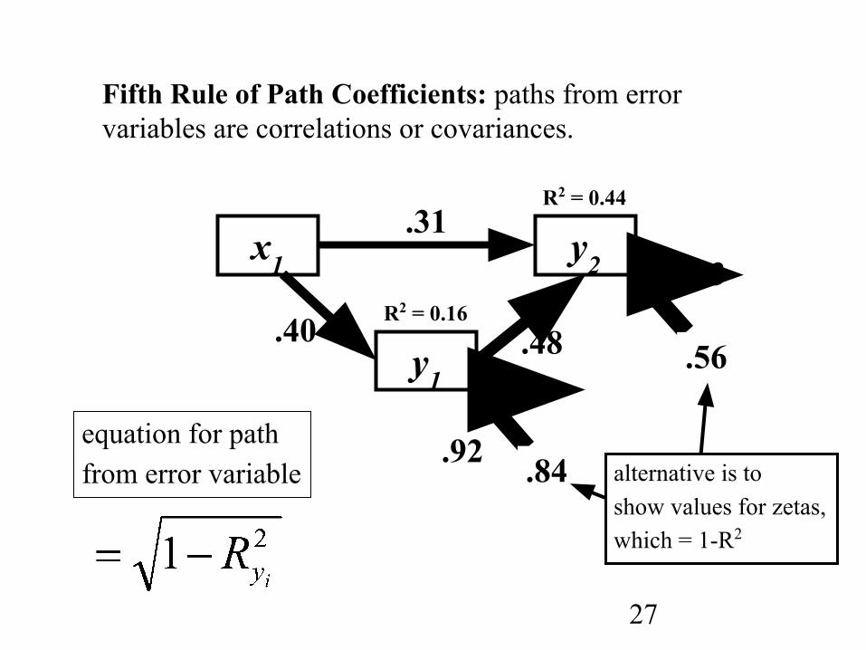
Fifth Rule of Path Coefficients: paths from error variables are correlations or covariances.

R2 = 0.16

.92

R2 = 0.44

.73

ζ2

ζ1

.31

.40 .48

equation for pathfrom error variable

.56

alternative is toshow values for zetas,which = 1-R2

.84

28

x1

y1

y2

R2 = 0.16

R2 = 0.25

ζ2

ζ1

.50

.40x1 y1 y2-------------------------------x1 1.0y1 0.40 1.0y2 0.50 0.60 1.0

Now, imagine y1 and y2 are joint responses

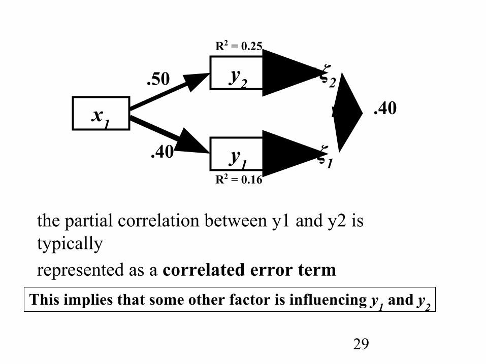
Sixth Rule of Path Coefficients: unanalyzed residual correlations between endogenous variables are partial correlations or covariances.

29

x1

y1

y2

R2 = 0.16

R2 = 0.25

ζ2

ζ1

.50

.40

.40

This implies that some other factor is influencing y1 and y2

the partial correlation between y1 and y2 is typicallyrepresented as a correlated error term

30

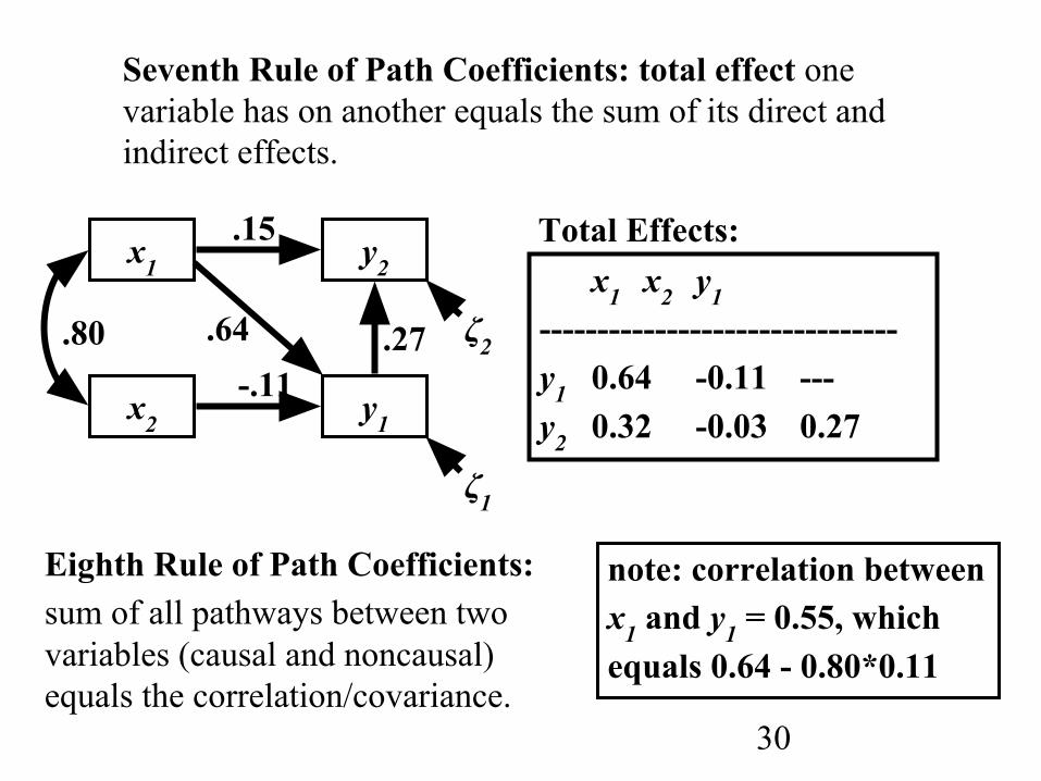
Seventh Rule of Path Coefficients: total effect one variable has on another equals the sum of its direct and indirect effects.

y1x2

x1 y2

ζ1

ζ2.80

.15

.64-.11

.27

x1 x2 y1-------------------------------y1 0.64 -0.11 ---y2 0.32 -0.03 0.27

Total Effects:

Eighth Rule of Path Coefficients:sum of all pathways between two variables (causal and noncausal) equals the correlation/covariance.

note: correlation betweenx1 and y1 = 0.55, which equals 0.64 - 0.80*0.11

31

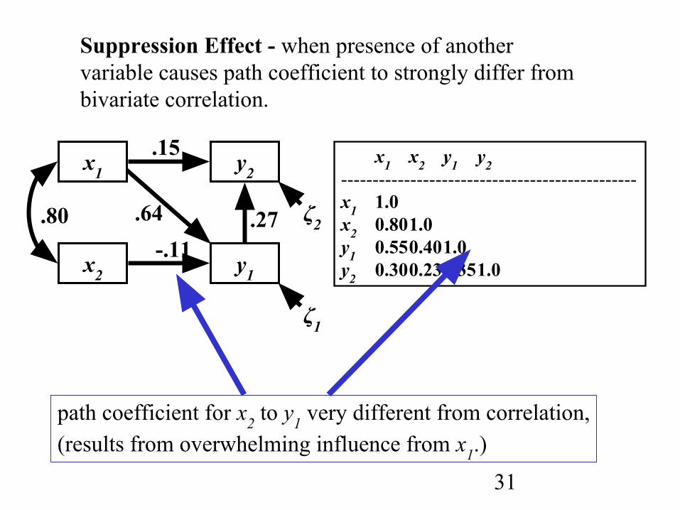
Suppression Effect - when presence of another variable causes path coefficient to strongly differ from bivariate correlation.

x1 x2 y1 y2 -----------------------------------------------x1 1.0x2 0.801.0y1 0.550.401.0y2 0.300.230.351.0y1x2

x1 y2

ζ1

ζ2.80

.15

.64-.11

.27

path coefficient for x2 to y1 very different from correlation,(results from overwhelming influence from x1.)

32


B. Anatomy of Latent Variable Models

33

Latent VariablesLatent variables are those whose presence we suspect or theorize, but for which we have no direct measures.

Intelligence IQ score

*note that we must specify some parameter, either error,loading, or variance of latent variable.

ζ

latent variable observed indicator errorvariable

1.0

fixed loading*

1.0

34

Latent Variables (cont.)

Purposes Served by Latent Variables:

(2) Allow us to estimate and correct for measurement error.

(3) Represent certain kinds of hypotheses.

(1) Specification of difference between observed data and processes of interest.

35

Range of Examples

single-indicator

Elevation

estimatefrom map

multi-method

SoilOrganic

soil C

loss onignitio

n

TerritorySize

singing range, t1

singing range, t2

singing range, t3

repeated measures

Caribou

Counts

observer 1

observer 2

repeatability

36

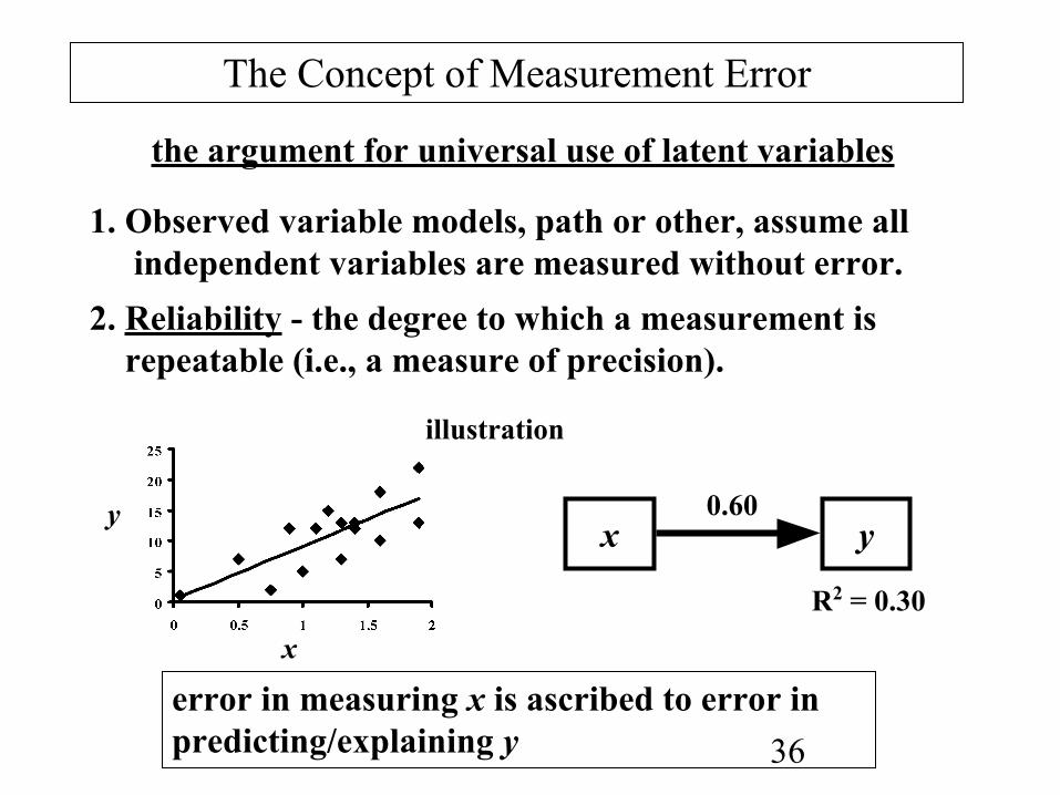
The Concept of Measurement Error

the argument for universal use of latent variables

1. Observed variable models, path or other, assume all independent variables are measured without error.2. Reliability - the degree to which a measurement is repeatable (i.e., a measure of precision).

error in measuring x is ascribed to error in predicting/explaining y

x y0.60

R2 = 0.30x

y

illustration

37

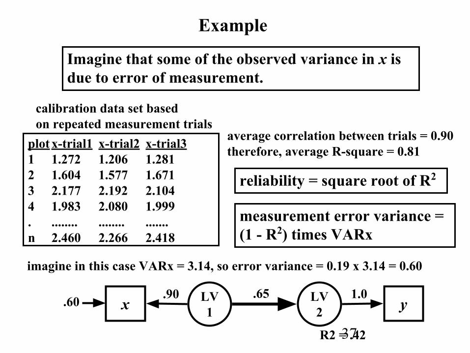
Example

Imagine that some of the observed variance in x is due to error of measurement.

calibration data set based on repeated measurement trials

plot x-trial1 x-trial2 x-trial31 1.272 1.206 1.2812 1.604 1.577 1.6713 2.177 2.192 2.1044 1.983 2.080 1.999. ........ ........ .......n 2.460 2.266 2.418

average correlation between trials = 0.90therefore, average R-square = 0.81

reliability = square root of R2

measurement error variance =(1 - R2) times VARx

imagine in this case VARx = 3.14, so error variance = 0.19 x 3.14 = 0.60

LV1x LV

2 y.90 .65 1.0.60

R2 = .42

38


C. Estimation and Evaluation

39

1. The Multiequational Framework

(a) the observed variable modelWe can model the interdependences among a set of predictors and responses using an extension of the general linear model that accommodates the dependences of response variables on other response variables.

y = p x 1 vector of responses

α = p x 1 vector of intercepts

Β = p x p coefficient matrix of ys on ys

Γ = p x q coefficient matrix of ys on xs

x = q x 1 vector of exogenous predictors

ζ = p x 1 vector of errors for the elements of y

Φ = cov (x) = q x q matrix of covariances among xs

Ψ = cov (ζ) = q x q matrix of covariances among errors

y = α + Βy + Γx + ζ

40

The LISREL Equations

Jöreskög 1973

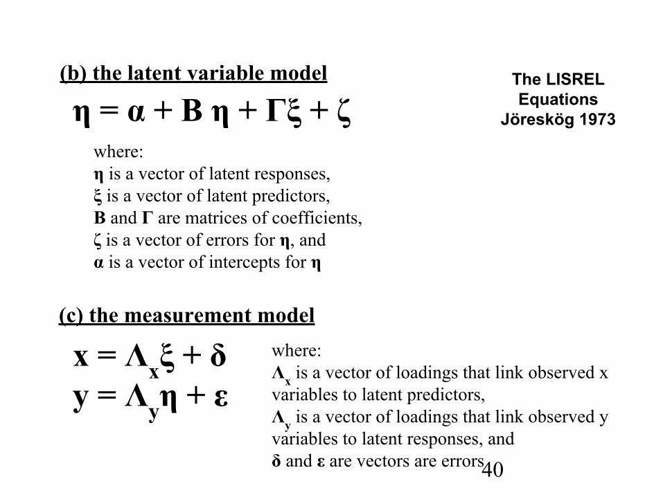
(b) the latent variable model

η = α + Β η + Γξ + ζ

x = Λxξ + δy = Λyη + ε

where: η is a vector of latent responses,ξ is a vector of latent predictors,Β and Γ are matrices of coefficients,ζ is a vector of errors for η, andα is a vector of intercepts for η

(c) the measurement modelwhere: Λx is a vector of loadings that link observed x variables to latent predictors,Λy is a vector of loadings that link observed y variables to latent responses, andδ and ε are vectors are errors

41

2. Estimation Methods

(a) decomposition of correlations (original path analysis)

(b) least-squares procedures (historic or in special cases)

(c) maximum likelihood (standard method)

(d) Markov chain Monte Carlo (MCMC) methods (including Bayesian applications)

42

Bayesian References:

Bayesian Networks: Neopolitan, R.E. (2004). Learning Bayesian Networks. Upper

Saddle River, NJ, Prentice Hall Publs.

Bayesian SEM: Lee, SY (2007) Structural Equation Modeling: A Bayesian

Approach. Wiley & Sons.

43

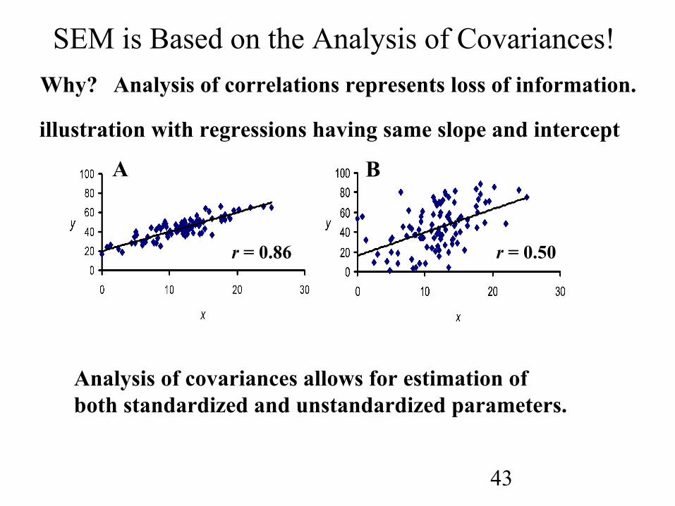
SEM is Based on the Analysis of Covariances!Why? Analysis of correlations represents loss of information.

A B

r = 0.86 r = 0.50

illustration with regressions having same slope and intercept

Analysis of covariances allows for estimation of both standardized and unstandardized parameters.

44

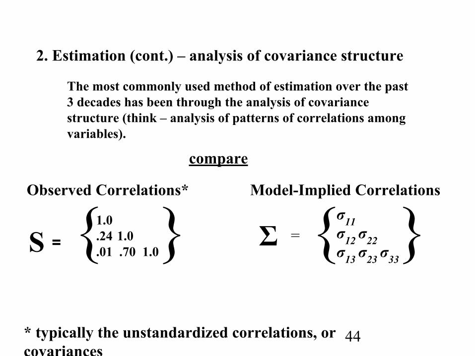
Σ = {σ11σ12 σ22σ13 σ23 σ33

}Model-Implied CorrelationsObserved Correlations*

{1.0.24 1.0.01 .70 1.0}S =

* typically the unstandardized correlations, or covariances

2. Estimation (cont.) – analysis of covariance structure

The most commonly used method of estimation over the past 3 decades has been through the analysis of covariance structure (think – analysis of patterns of correlations among variables).

compare

45

x1

y1

y2

Hypothesized Model

Σ = {σ11σ12 σ22σ13 σ23 σ33

}Implied Covariance Matrix

Observed Covariance Matrix

{1.3.24 .41.01 9.7 12.3}S =

compareModel FitEvaluations

+

ParameterEstimates

estimation

(e.g., maximum likelihood)

3. Evaluation

46

Model Identification - Summary

2. Several factors can prevent identification, including:a. too many paths specified in modelb. certain kinds of model specifications can make parameters unidentifiedc. multicollinearityd. combination of a complex model and a small sample

1. For the model parameters to be estimated with unique values, they must be identified. As in linear algebra, we have a requirement that we need as many known pieces of information as we do unknown parameters.

3. Good news is that most software checks for identification (in something called the information matrix) and lets you know which parameters are not identified.

47

The most commonly used fitting function in maximum likelihood estimation of structural equation models is based on the log likelihood ratio, which compares the likelihood for a given model to the likelihood of a model with perfect fit.

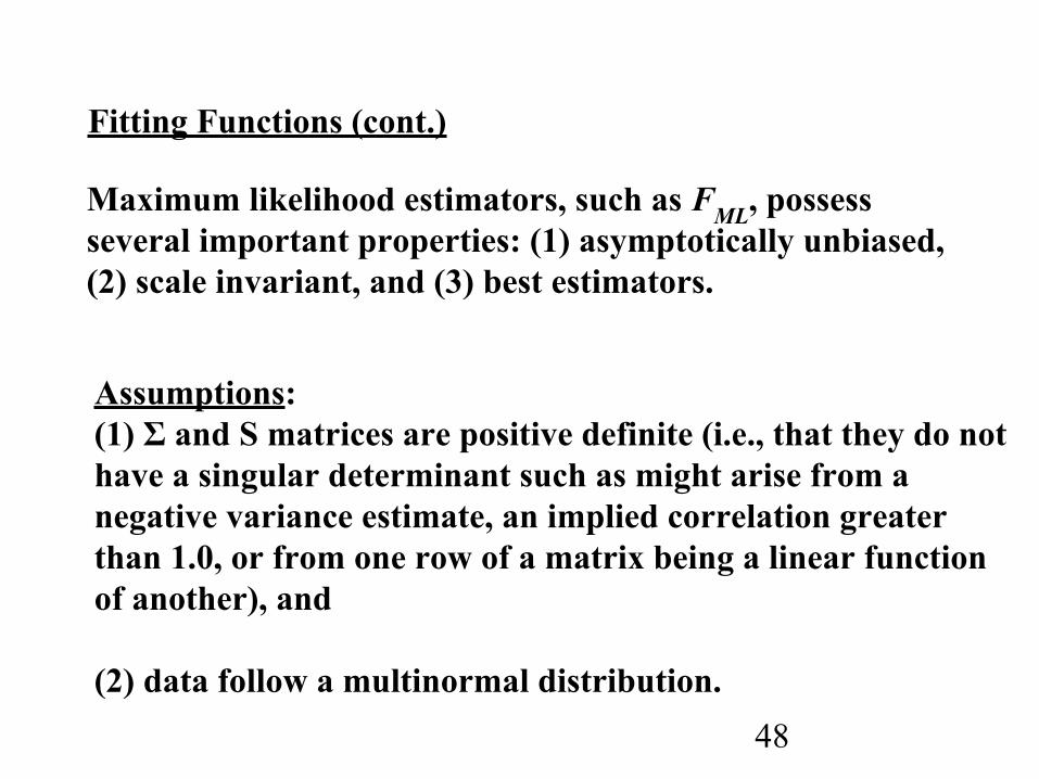
Fitting Functions

Note that when sample matrix and implied matrix are equal, terms 1 and 3 = 0 and terms 2 and 4 = 0. Thus, perfect model fit yields a value of FML of 0.

48

Maximum likelihood estimators, such as FML, possess several important properties: (1) asymptotically unbiased, (2) scale invariant, and (3) best estimators.

Assumptions: (1) Σ and S matrices are positive definite (i.e., that they do not have a singular determinant such as might arise from a negative variance estimate, an implied correlation greater than 1.0, or from one row of a matrix being a linear function of another), and

(2) data follow a multinormal distribution.

Fitting Functions (cont.)

49

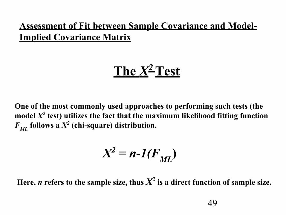
One of the most commonly used approaches to performing such tests (the model Χ2 test) utilizes the fact that the maximum likelihood fitting function FML follows a X2 (chi-square) distribution.

The Χ2 Test

X2 = n-1(FML)

Here, n refers to the sample size, thus X2 is a direct function of sample size.

Assessment of Fit between Sample Covariance and Model- Implied Covariance Matrix

50

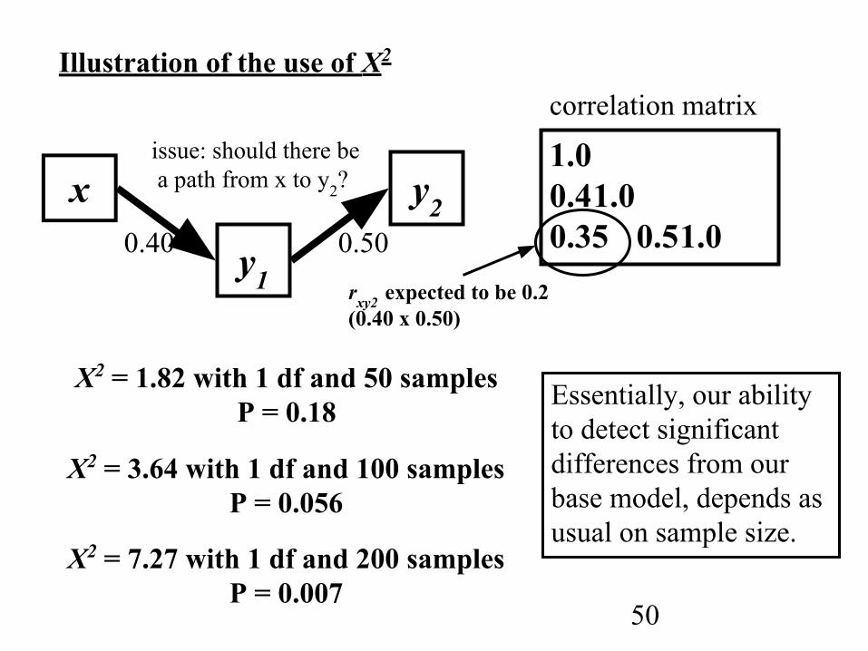
Illustration of the use of Χ2

X2 = 3.64 with 1 df and 100 samplesP = 0.056


x

y1

y2

1.00.41.00.35 0.51.0

rxy2 expected to be 0.2 (0.40 x 0.50)


correlation matrixissue: should there be a path from x to y2?

0.40 0.50

Essentially, our ability to detect significant differences from our base model, depends as usual on sample size.

51

Additional Points about Model Fit Indices:

1.The chi-square test appears to be reasonably effective at sample sizes less than 200.

2. There is no perfect answer to the model selection problem.

4. A lot of attention is being paid to Bayesian model selection methods at the present time.

3. No topic in SEM has had more attention than the development of indices that can be used as guides for model selection.

5. In SEM practice, much of the weight of evidence falls on the investigator to show that the results are repeatable (predictive of the next sample).

52

Alternatives when data extremely nonnormal

Robust Methods: Satorra, A., & Bentler, P. M. (1988). Scaling corrections for

chi-square statistics in covariance structure analysis. 1988 Proceedings of the Business and Economics Statistics Section of the American Statistical Association, 308-313.

Bootstrap Methods:Bollen, K. A., & Stine, R. A. (1993). Bootstrapping

goodness-of-fit measures in structural equation models. In K. A. Bollen and J. S. Long (Eds.) Testing structural equation models. Newbury Park, CA: Sage Publications.

Alternative Distribution Specification: - Bayesian and other:

53

Residuals: Most fit indices represent average of residuals between observed and predicted covariances. Therefore, individual residuals should be inspected.

Correlation Matrix to be Analyzed y1 y2 x -------- -------- --------y1 1.00y2 0.50 1.00 x 0.40 0.35 1.00

Fitted Correlation Matrix y1 y2 x -------- -------- --------y1 1.00y2 0.50 1.00 x 0.40 0.20 1.00

residual = 0.15

Diagnosing Causes of Lack of Fit (misspecification)

Modification Indices: Predicted effects of model modification on model chi-square.

54

The topic of model selection, which focuses on how you choose among competing models, is very important. Please refer to additional tutorials for considerations of this topic.

55

While we have glossed over as many details as we could, these fundamentals will hopefully help you get started with SEM.

Another gentle introduction to SEM oriented to the community ecologist is Chapter 30 in McCune, B. and J.B. Grace 2004. Analysis of Ecological Communities. MJM. (sold at cost with no profit)

(sem) essentials structural equation...

Documents