Semantic Segmentation using Adversarial Networks

Pauline LucFacebook AI Research

Paris, France

Camille CouprieFacebook AI Research

Paris, France

Soumith ChintalaFacebook AI Research

New York, USA

Jakob VerbeekINRIA, Laboratoire Jean Kuntzmann

Grenoble, France

Abstract

Adversarial training has been shown to produce state of the art results for generativeimage modeling. In this paper we propose an adversarial training approach to trainsemantic segmentation models. We train a convolutional semantic segmentationnetwork along with an adversarial network that discriminates segmentation mapscoming either from the ground truth or from the segmentation network. The moti-vation for our approach is that it can detect and correct higher-order inconsistenciesbetween ground truth segmentation maps and the ones produced by the segmen-tation net. Our experiments show that our adversarial training approach leads toimproved accuracy on the Stanford Background and PASCAL VOC 2012 datasets.

1 Introduction

Semantic segmentation is a visual scene understanding task formulated as a dense labeling problem,where the goal is to predict a category label at each pixel in the input image. Current state-of-the-artmethods [2, 15, 16, 21] rely on convolutional neural network (CNN) approaches, following earlywork using CNNs for this task by Grangier et al . in 2009 [11] and Farabet et al . [7] in 2013. Despitemany differences in the CNN architectures, a common property across all these approaches is that alllabel variables are predicted independently from each other. This is the case at least during training;various post-processing approaches have been explored to reinforce spatial contiguity in the outputlabel maps since the independent prediction model does not capture this explicitly.

Conditional Markov random fields (CRFs) are one of the most effective approaches to enforcespatial contiguity in the output label maps. The CNN-based approaches mentioned above can beused to define unary potentials. For certain classes of pairwise potentials, mean-field inference infully-connected CRFs with millions of variables is tractable using recent filter-based techniques[14].Such fully-connected CRFs have been found extremely effective in practice to recover fine details inthe output maps. Moreover, using a recurrent neural network formulation [30, 35] of the mean-fielditerations, it is possible to train the CNN underlying the unary potentials in an integrated mannerthat takes into account the CRF inference during training. It has also been shown that a rich class ofpairwise potentials can be learned using CNN techniques in locally connected CRFs [15].

Despite these advances, the work discussed above is limited to the use of pairwise CRF models.Higher-order potentials, however, have also been observed to be effective, for example robust higher-order terms based on label consistency across superpixels [13]. Recent work [1] has shown how

Workshop on Adversarial Training, NIPS 2016, Barcelona, Spain.

arX

iv:1

611.

0840

8v1

[cs

.CV

] 2

5 N

ov 2

016

Segmentor Adversarial network

Image

Class predic-tions

Convnet

concat

0 or 1 prediction

Ground truth

or

1664

128 256 512

64

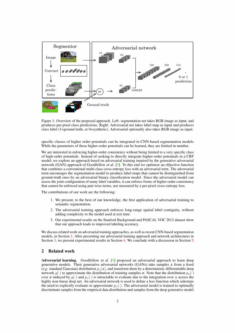
Figure 1: Overview of the proposed approach. Left: segmentation net takes RGB image as input, andproduces per-pixel class predictions. Right: Adversarial net takes label map as input and producesclass label (1=ground truth, or 0=synthetic). Adversarial optionally also takes RGB image as input.

specific classes of higher order potentials can be integrated in CNN-based segmentation models.While the parameters of these higher-order potentials can be learned, they are limited in number.

We are interested in enforcing higher-order consistency without being limited to a very specific classof high-order potentials. Instead of seeking to directly integrate higher-order potentials in a CRFmodel, we explore an approach based on adversarial training inspired by the generative adversarialnetwork (GAN) approach of Goodfellow et al . [9]. To this end we optimize an objective functionthat combines a conventional multi-class cross-entropy loss with an adversarial term. The adversarialterm encourages the segmentation model to produce label maps that cannot be distinguished fromground-truth ones by an adversarial binary classification model. Since the adversarial model canassess the joint configuration of many label variables, it can enforce forms of higher-order consistencythat cannot be enforced using pair-wise terms, nor measured by a per-pixel cross-entropy loss.

The contributions of our work are the following:

1. We present, to the best of our knowledge, the first application of adversarial training tosemantic segmentation.

2. The adversarial training approach enforces long-range spatial label contiguity, withoutadding complexity to the model used at test time.

3. Our experimental results on the Stanford Background and PASCAL VOC 2012 dataset showthat our approach leads to improved labeling accuracy.

We discuss related work on adversarial training approaches, as well as recent CNN-based segmentationmodels, in Section 2. After presenting our adversarial training approach and network architectures inSection 3, we present experimental results in Section 4. We conclude with a discussion in Section 5.

2 Related work

Adversarial learning. Goodfellow et al . [9] proposed an adversarial approach to learn deepgenerative models. Their generative adversarial networks (GANs) take samples z from a fixed(e.g . standard Gaussian) distribution pz(z), and transform them by a deterministic differentiable deepnetwork g(·) to approximate the distribution of training samples x. Note that the distribution px(·)over x induced by g(·) and pz(·) is intractable to evaluate due to the integration over z across thehighly non-linear deep net. An adversarial network is used to define a loss function which sidestepsthe need to explicitly evaluate or approximate px(·). The adversarial model is trained to optimallydiscriminate samples from the empirical data distribution and samples from the deep generative model.

2

The generative model is concurrently trained to minimize accuracy of the adversarial, which provablydrives the generative model to approximate the distribution of the training data. The adversarial netcan be interpreted as a “variational” loss function, in the sense that the loss function of the generativemodel is defined by auxiliary parameters that are not part of the generative model.

In follow-up work, Radford et al . [25] present a number of architectural design choices that enablestable training of generative models that are able to synthesize realistic images. Similar to Goodfellowet al . [9], they use deep “deconvolutional” networks g(·) that progressively construct the image byup-sampling, using essentially a reverse CNN architecture. Denton et al . [4] use a Laplacian pyramidapproach to learn a sequence of GAN models that successively generate images with finer details.Extensions of GANs for conditional modeling have been explored, e.g . for image tag prediction [19],face image generation conditioned on attributes [8], and for caption-based image synthesis [26].

Deep conditional generative models have also been defined in a non-stochastic manner, where for agiven conditioning variable a single deterministic output is generated. For example, Dosovitskiy etal . [5] developed deep generative image models where the conditioning variables encode the objectclass, viewpoint, and color-related transformations. In this case a conventional regression loss can beused, since inference or integration on the conditioning variables is not needed. Dosovitskiy et al .train their models using an `2 regression loss on the target images.

In other examples the conditioning variable takes the form of one or more input images. Mathieuet al . [18] considered the problem of predicting the next frame in video given several precedingframes. Pathak et al . [22] considered the problem of image inpainting, where the missing part ofthe images has to be predicted from the observed part. Such models are closely related to deepconvolutional semantic segmentation models that deterministically produce a label probability map,conditioned on an input RGB image. In the latter two cases, a regression loss in combined withan adversarial loss term. The motivation in both cases is that per-pixel regression losses typicallyresult in too blurry outputs, since they do not for higher-order regularities in the output. Sincethe adversarial net has access to large portions or the entire output image, it can be interpreted asa learned higher-order loss, which obviates the need to manually design higher-order loss terms.The work of Tarlow and Zemel [33] is related to this approach as they also suggested to learn withhigher-order loss terms, while not including such higher-order terms in the predictive model to ensureefficient prediction. Several authors have shown that images on which convolutional classificationnetworks produce confident but incorrect predictions can be found by manipulating natural imagesin a human-imperceptible manner [32], or by synthesizing non-natural images [20]. This is relatedto adversarial training in the sense that they seek to reduce the CNN performance by perturbing theinput, in GANs these perturbations are further back-propagated through the generative network toimprove its performance.

Semantic segmentation. While early CNN-based semantic segmentation approaches were explic-itly passing image patches through the CNN, see e.g . [7], current state-of-the-art method indifferentlyuse a fully convolutional approach [16]. This is far more efficient, since it avoids redundant computa-tion of low-level filters many times on pixels in overlapping patches. Typical architectures involve anumber of pooling steps, which can increase the receptive field size rapidly after several steps. As aresult, however, the resolution of the output maps reduces, which means that a low-resolution labelmap is obtained. To address this issue, the signal can be up-sampled using bi-linear interpolation, orlearned up-sampling filters [16, 21, 27]. Alternatively, one can use dilated convolutions to increasethe receptive field size without losing resolution [2, 34], skip connections to earlier high-resolutionlayers [16, 27], or multi-resolution networks [29, 36].

Most work that combines CNN unary label predictions with CRFs is based on models with pairwiseor higher-order terms with few trainable parameters [1, 30, 35]. An exception is the work of Linet al . [15] which uses a second CNN to learn data dependent pairwise terms. Another approachthat exploits high-capacity trainable models to drive long-range label interactions is to use recurrentnetworks [23], where each iteration maps the input image and current label map to a new label map.

In comparison to these previous approaches our work has the following merits: (i) The adversarialmodel has a high capacity, and is thus flexible enough to detect mismatches in a wide range of higher-order statistics between the model predictions and the ground-truth, without having to manuallydefine these. (ii) Once trained, our model is efficient since it does not involve any higher-order termsor recurrence in the model itself.

3

3 Adversarial training for semantic segmentation networks

We describe our general framework for adversarial training of semantic segmentation models inSection 3.1. We present the architectures used in our experiments in Section 3.2.

3.1 Adversarial training

We propose to use a hybrid loss function that is a weighted sum of two terms. The first is a multi-classcross-entropy term that encourages the segmentation model to predict the right class label at eachpixel location independently. This loss is standard in state-of-the-art semantic segmentation models,see e.g. [2, 15, 16, 21]. We use s(x) to denote the class probability map over C classes of sizeH ⇥W ⇥C that the segmentation model produces given an input RGB image x of size H ⇥W ⇥ 3.

The second loss term is based on an auxiliary adversarial convolutional network. This loss termis large if the adversarial network can discriminate the output of the segmentation network fromground-truth label maps. Since the adversarial CNN has a field-of-view that is either the entireimage or a large portion of it, mismatches in the higher-order label statistics can be penalized by theadversarial loss term. Higher-order label statistics (such as e.g . the shape of a region of pixels labeledwith a certain class, or whether the fraction of pixels in a region of a certain class exceeds a threshold)are not accessible by the standard per-pixel factorized loss function. We use a(x, y) 2 [0, 1] todenote the scalar probability with which the adversarial model predicts that y is the ground truthlabel map of x, as opposed to being a label map produced by the segmentation model s(·).Given a data set of N training images xn and a corresponding label maps yn, we define the loss as

`(✓s,✓a) =NX

n=1

`mce(s(xn), yn) � �h`bce(a(xn, yn), 1) + `bce(a(xn, s(xn)), 0)

i, (1)

where ✓s and ✓a denote the parameters of the segmentation model and adversarial model respectively.In the above, `mce(y, y) = �PH⇥W

i=1

PCc=1 yic ln yic denotes the multi-class cross-entropy loss for

predictions y, which equals the negative log-likelihood of the target segmentation map y representedusing a 1-hot encoding. Similarly, we use `bce(z, z) = �

⇥z ln z + (1 � z) ln(1 � z)

⇤, the binary

cross-entropy loss. We minimize the loss with respect to the parameters ✓s of the segmentationmodel, while maximizing it w.r.t. the parameters ✓a of the adversarial model.

Training the adversarial model. Since only the second term depends on the adversarial model,training the adversarial model is equivalent to minimizing the following binary classification loss

NX

n=1

`bce(a(xn, yn), 1) + `bce(a(xn, s(xn)), 0). (2)

In our experiments we let a(·) take the form of a CNN. Below, in Section 3.2, we describe severalvariants for the adversarial network’s architecture, exploring different possibilities for the combinationof the inputs and the field-of-view of the adversarial network.

Training the segmentation model. Given the adversarial network, the training of the segmentationmodel minimizes the multi-class cross-entropy loss, while at the same time degrading the performanceof the adversarial model. This encourages the segmentation model to produce segmentation maps thatare hard to distinguish from ground-truth ones for the adversarial model. The terms of the objectivefunction Eq. (1) relevant to the segmentation model are

NX

n=1

`mce(s(xn), yn) � �`bce(a(xn, s(xn)), 0) (3)

We follow Goodfellow et al . [9], and replace the term ��`bce(a(xn, s(xn)), 0) with+�`bce(a(xn, s(xn)), 1) when updating the segmentation model in practice. In other words: in-stead of minimizing the probability that the adversarial predicts s(xn) to be synthetic label mapfor xn, we maximize the probability that the adversarial predicts it to be a ground truth map forxn. It is easy to show that `bce(a(xn, s(xn)), 0) and �`bce(a(xn, s(xn)), 1) share the same set of

4

critical points. The rationale for this modified update is that it leads to a stronger gradient signal whenthe adversarial makes accurate predictions on the synthetic/ground-truth nature of the label maps.Preliminary experiments confirmed that this is indeed important in practice to speedup training.

3.2 Network architectures

We now detail the architectures we used for our preliminary experiments on the Stanford Backgrounddataset and large-scale experiments on the PASCAL VOC 2012 segmentation benchmark.

Stanford Background dataset. For this dataset we used the multi-scale segmentation network ofFarabet et al . [7], and train it patch-wise from scratch. The adversarial takes as input a label map,and the corresponding RGB image. The label map is either the ground truth corresponding to theimage, or produced by the segmentation net. The ground truth label maps are down-sampled to matchthe output resolution of the segmentation net, and fed in a 1-hot encoding to the adversarial. Thearchitecture of the adversarial is similar to that illustrated in Figure 1, its precise details are given inthe supplementary material. At first, two separate branches process the image and the label map, toallow different low level representations for the two different signals. We follow the observation ofPinheiro et al . [24] that it is preferable to have roughly the same number of channels for each inputsignal, so as to avoid that one signal dominates the other when fed to subsequent layers. When fusingthe two signal branches, we represent both inputs using 64 channels. The signals are then passedinto another stack of convolutional and max-pooling layers, after which the binary class probabilityis produced by a sigmoid activation. The adversarial network applies two max-pooling operatorsto the label maps, resulting in a number synthetic/ground-truth predictions of the adversarial that is4 ⇥ 4 = 16 times smaller than the number of predictions generated by the segmentation network.

Pascal VOC 2012 dataset. For this dataset we used the state-of-the-art Dilated-8 architecture ofYu et al . [34], and fine-tune the pre-trained model. This architecture is built upon the VGG-16architecture [31], but does not include the two last max-pooling layers to maintain a higher resolution.The convolutions that follow the modified pooling operators are dilated with a factor of two foreach preceding suppressed max-pooling layer. Following the last convolutional layer, a “contextmodule” composed of eight convolutional layers with increasing dilation factors, is used to expandthe network’s field-of-view while maintaining the resolution of the feature maps. We explore threevariants for the adversarial network input, which we call respectively Basic, Product and Scaling.

In the first approach, Basic, we directly input the probability maps generated by the segmentationnetwork. Preliminary experiments in this set-up show no difference when adding the correspondingRGB image, we therefore do not use it for simplicity. One concern for this choice of the inputs isthat the adversarial network can potentially trivially distinguish the ground truth and generated labelmaps by detecting if the map consists of zeros and ones (one-hot coding of ground truth), or of valuesbetween zero and one (output of segmentation network).

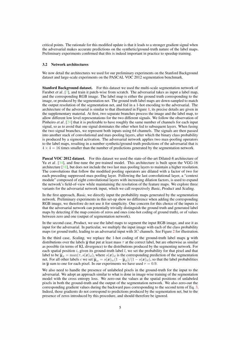
In the second case, Product, we use the label maps to segment the input RGB image, and use it asinput for the adversarial. In particular, we multiply the input image with each of the class probabilitymaps (or ground truth), leading to an adversarial input with 3C channels. See Figure 2 for illustration.

In the third case, Scaling, we replace the 1-hot coding of the ground-truth label maps y withdistributions over the labels y that put at least mass ⌧ at the correct label, but are otherwise as similaras possible (in terms of KL divergence) to the distributions produced by the segmenting network. Foreach spatial position i, given its ground-truth label l, we set the probability for that pixel and thatlabel to be yil = max(⌧, s(x)il), where s(x)il is the corresponding prediction of the segmentationnet. For all other labels c we set yic = s(x)ic(1 � yil)/(1 � s(x)il), so that the label probabilitiesin y sum to one for each pixel. In our experiments we have used ⌧ = 0.9.

We also need to handle the presence of unlabeled pixels in the ground-truth for the input to theadversarial. We adopt an approach similar to what is done in image-wise training of the segmentationmodel with the cross entropy loss. We zero-out the values at the spatial positions of unlabeledpixels in both the ground-truth and the output of the segmentation network. We also zero-out thecorresponding gradient values during the backward pass corresponding to the second term of Eq. 3.Indeed, those gradients do not correspond to predictions produced by the segmentation net, but to thepresence of zeros introduced by this procedure, and should therefore be ignored.

5

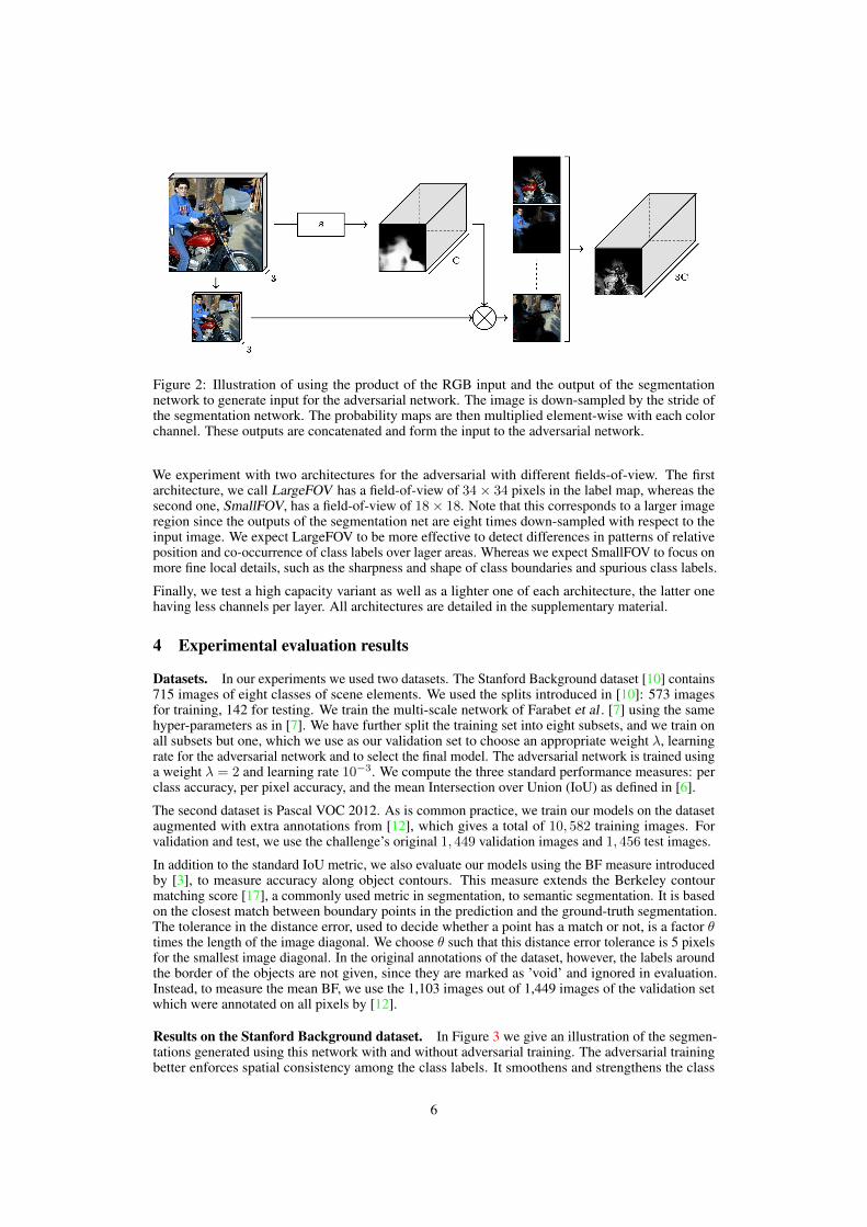
Figure 2: Illustration of using the product of the RGB input and the output of the segmentationnetwork to generate input for the adversarial network. The image is down-sampled by the stride ofthe segmentation network. The probability maps are then multiplied element-wise with each colorchannel. These outputs are concatenated and form the input to the adversarial network.

We experiment with two architectures for the adversarial with different fields-of-view. The firstarchitecture, we call LargeFOV has a field-of-view of 34 ⇥ 34 pixels in the label map, whereas thesecond one, SmallFOV, has a field-of-view of 18 ⇥ 18. Note that this corresponds to a larger imageregion since the outputs of the segmentation net are eight times down-sampled with respect to theinput image. We expect LargeFOV to be more effective to detect differences in patterns of relativeposition and co-occurrence of class labels over lager areas. Whereas we expect SmallFOV to focus onmore fine local details, such as the sharpness and shape of class boundaries and spurious class labels.

Finally, we test a high capacity variant as well as a lighter one of each architecture, the latter onehaving less channels per layer. All architectures are detailed in the supplementary material.

4 Experimental evaluation results

Datasets. In our experiments we used two datasets. The Stanford Background dataset [10] contains715 images of eight classes of scene elements. We used the splits introduced in [10]: 573 imagesfor training, 142 for testing. We train the multi-scale network of Farabet et al . [7] using the samehyper-parameters as in [7]. We have further split the training set into eight subsets, and we train onall subsets but one, which we use as our validation set to choose an appropriate weight �, learningrate for the adversarial network and to select the final model. The adversarial network is trained usinga weight � = 2 and learning rate 10�3. We compute the three standard performance measures: perclass accuracy, per pixel accuracy, and the mean Intersection over Union (IoU) as defined in [6].

The second dataset is Pascal VOC 2012. As is common practice, we train our models on the datasetaugmented with extra annotations from [12], which gives a total of 10, 582 training images. Forvalidation and test, we use the challenge’s original 1, 449 validation images and 1, 456 test images.

In addition to the standard IoU metric, we also evaluate our models using the BF measure introducedby [3], to measure accuracy along object contours. This measure extends the Berkeley contourmatching score [17], a commonly used metric in segmentation, to semantic segmentation. It is basedon the closest match between boundary points in the prediction and the ground-truth segmentation.The tolerance in the distance error, used to decide whether a point has a match or not, is a factor ✓times the length of the image diagonal. We choose ✓ such that this distance error tolerance is 5 pixelsfor the smallest image diagonal. In the original annotations of the dataset, however, the labels aroundthe border of the objects are not given, since they are marked as ’void’ and ignored in evaluation.Instead, to measure the mean BF, we use the 1,103 images out of 1,449 images of the validation setwhich were annotated on all pixels by [12].

Results on the Stanford Background dataset. In Figure 3 we give an illustration of the segmen-tations generated using this network with and without adversarial training. The adversarial trainingbetter enforces spatial consistency among the class labels. It smoothens and strengthens the class

6

sky tree road grass water building mountain fg. object

input ground truth no adversarial with adversarial

Figure 3: Segmentations on Stanford Background. Class probabilities without (first row) and with(second row) adversarial training. In the last row the class labels are superimposed on the image.

0 200 400 600 800 1,000

50

60

70

80

90

Number of epochs

Tra

inin

gper

class

accu

racy

Classical trainingUsing adversarial training

0 200 400 600 800 1,000

56

58

60

62

64

66

Number of epochs

Val

idat

ion

per

clas

sac

cura

cy

Classical trainingUsing adversarial training

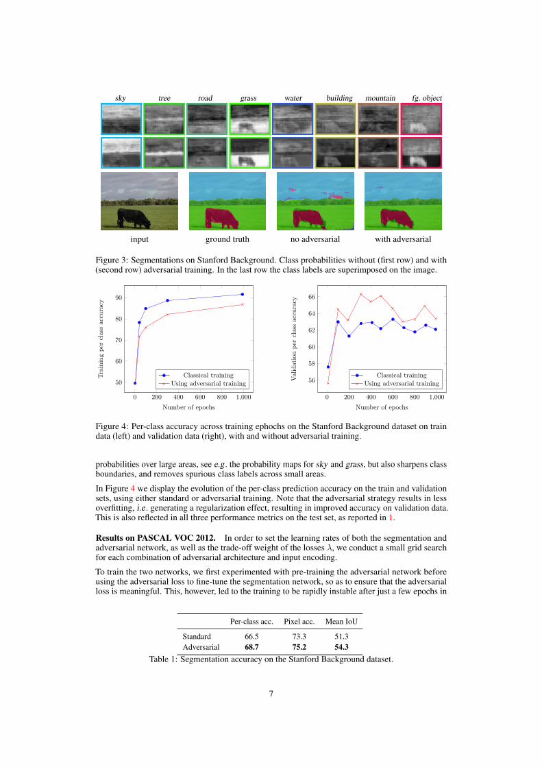
Figure 4: Per-class accuracy across training ephochs on the Stanford Background dataset on traindata (left) and validation data (right), with and without adversarial training.

probabilities over large areas, see e.g . the probability maps for sky and grass, but also sharpens classboundaries, and removes spurious class labels across small areas.

In Figure 4 we display the evolution of the per-class prediction accuracy on the train and validationsets, using either standard or adversarial training. Note that the adversarial strategy results in lessoverfitting, i.e . generating a regularization effect, resulting in improved accuracy on validation data.This is also reflected in all three performance metrics on the test set, as reported in 1.

Results on PASCAL VOC 2012. In order to set the learning rates of both the segmentation andadversarial network, as well as the trade-off weight of the losses �, we conduct a small grid searchfor each combination of adversarial architecture and input encoding.

To train the two networks, we first experimented with pre-training the adversarial network beforeusing the adversarial loss to fine-tune the segmentation network, so as to ensure that the adversarialloss is meaningful. This, however, led to the training to be rapidly instable after just a few epochs in

Per-class acc. Pixel acc. Mean IoU

Standard 66.5 73.3 51.3Adversarial 68.7 75.2 54.3

Table 1: Segmentation accuracy on the Stanford Background dataset.

7

Basic Product Scaling

mIOU mBF mIOU mBF mIOU mBF

LargeFOV 72.0 47.2 72.0 47.7 72.0 47.9SmallFOV 72.0 47.6 71.9 46.4 71.9 47.1LargeFOV-light 72.0 47.0 72.0 47.7 72.0 47.4SmallFOV-light 71.9 47.2 71.9 47.4 72.0 46.9

Table 2: Performance using different architectures and input encodings for the adversarial model.

many experiments. We found that training instead using an alternating scheme is more effective. Weexperimented with a fast alternating scheme, where we alternate between updating the segmentingnetwork’s and the adversarial network’s weights at every iteration of SGD and a slow one, wherewe alternate only after 500 iterations of each. We found the second scheme to led to the most stabletraining, and used it for the results reported in Table 2. For details on the hyper-parameter search, andthe final hyper-parameters used for each model, we refer the reader to the supplementary material.

We compare the results of adversarial training with a baseline consisting of fine-tuning of Dilated8using the cross-entropy loss only. For the baseline we obtained a mean IoU of 71.8 and mean BF of47.4. As shown in Table 2, we observe small but consistent gains for most adversarial training setups.In particular, the LargeFOV architecture is the most effective overall. Moreover, it is interesting tonote that the different adversarial input encodings lead to comparable results. In fact, we found thatfor the basic input encoding, the adversarial does not succeed in perfectly separating ground-truthand predicted label maps, it rather has a discrimination accuracy that is comparable to that obtainedwith the other input encodings.

Using the evaluation server we also tested selected models on the PASCAL VOC 2012 test set. Forthe baseline model we obtain (73.1), while for LargeFOV-Product and LargeFOV-Scaling we obtained73.3 and 73.2 respectively. This confirms the small but consistent gains that we observed on thevalidation data.

5 Discussion

We have presented an adversarial approach to learn semantic segmentation models. In the originalwork of Goodfellow et al . [9] the adversarial model is used to define a proxy loss for a generativemodel in which the calculation of the cross-entropy loss is intractable. In contrast, the CNN-basedsegmentation models we use allow for tractable computation of the exact multi-class cross-entropyloss. In our work we use the adversarial network as a “variational” loss, with adjustable parameters, toregularize the segmentation model by enforcing higher-order consistency in the factorized predictionmodel of the label variables. Methodologically, this approach is related to work by Roweis etal . [28], where variational inference was used in tractable linear-Gaussian mixture models to enforceconsistency across multiple local dimension reduction models, and to work by Tarlow and Zemel [33]which learn models with higher-order loss terms, while not including such higher-order terms in thepredictive model to ensure efficient inference.

To demonstrate the regularization property of adversarial training, we conducted experiments onthe Standford Background dataset and the PASCAL VOC 2012 dataset. Our results show that theadversarial training approach leads to improvements in semantic segmentation accuracy on bothdatasets. The gains in accuracy observed on the Stanford Background dataset are more pronounced.This is most likely due to higher risk of over fitting using this smaller data set, and also due to themore powerful segmentation architectures used for the PASCAL VOC 2012 dataset.

Acknowledgments

This work has been partially supported by the LabEx PERSYVAL-Lab (ANR-11-LABX-0025-01).

8

References[1] A. Arnab, S. Jayasumana, S. Zheng, and P. Torr. Higher order conditional random fields in deep neural

networks. In ECCV, 2016.[2] L.-C. Chen, G. Papandreou, I. Kokkinos, K. Murphy, and A. Yuille. Semantic image segmentation with

deep convolutional nets and fully connected CRFs. In ICLR, 2015.[3] G. Csurka, D. Larlus, and F. Perronnin. What is a good evaluation measure for semantic segmentation? In

BMVC, 2013.[4] E. Denton, S. Chintala, A. Szlam, and R. Fergus. Deep generative image models using a Laplacian pyramid

of adversarial networks. In NIPS, 2015.[5] A. Dosovitskiy, J. Springenberg, and T. Brox. Learning to generate chairs with convolutional neural

networks. In CVPR, 2015.[6] M. Everingham, S. Ali Eslami, L. van Gool, C. Williams, J. Winn, and A. Zisserman. The PASCALvisual

object classes challenge: A retrospective. IJCV, 111(1):98–136, 2015.[7] C. Farabet, C. Couprie, L. Najman, and Y. LeCun. Learning hierarchical features for scene labeling. PAMI,

35(8):1915–1929, 2013.[8] J. Gauthier. Conditional generative adversarial nets for convolutional face generation. Unpublished,

.[9] I. Goodfellow, J. Pouget-Abadie, M. Mirza, B. Xu, D. Warde-Farley, S. Ozair, A. Courville, and Y. Bengio.

Generative adversarial nets. In NIPS, 2014.[10] S. Gould, R. Fulton, and D. Koller. Decomposing a scene into geometric and semantically consistent

regions. In ICCV, 2009.[11] D. Grangier, L. Bottou, and R. Collobert. Deep convolutional networks for scene parsing. In ICML Deep

Learning Workshop, 2009.[12] B. Hariharan, P. Arbelaez, L. Bourdev, S. Maji, and J. Malik. Semantic contours from inverse detectors. In

ICCV, 2011.[13] P. Kohli, L. Ladický, and P. Torr. Robust higher order potentials for enforcing label consistency. IJCV,

82(3):302–324, 2009.[14] P. Krähenbühl and V. Koltun. Parameter learning and convergent inference for dense random fields. In

ICML, 2013.[15] G. Lin, C. Shen, A. van den Hengel, and I. Reid. Efficient piecewise training of deep structured models for

semantic segmentation. In CVPR, 2016.[16] J. Long, E. Shelhamer, and T. Darrell. Fully convolutional networks for semantic segmentation. In CVPR,

2015.[17] D. Martin, C. Fowlkes, and J. Malik. Learning to detect natural image boundaries using local brightness,

color, and texture cues. PAMI, 26(5):530–549, 2004.[18] M. Mathieu, C. Couprie, and Y. LeCun. Deep multi-scale video prediction beyond mean square error. In

ICLR, 2016.[19] M. Mirza and S. Osindero. Conditional generative adversarial nets. In NIPS deep learning workshop, 2014.[20] A. Nguyen, J. Yosinski, and J. Clune. Deep neural networks are easily fooled: High confidence predictions

for unrecognizable images. In CVPR, 2015.[21] H. Noh, S. Hong, and B. Han. Learning deconvolution network for semantic segmentation. In ICCV, 2015.[22] D. Pathak, P. Krähenbühl, J. Donahue, T. Darrell, and A. Efros. Context encoders: Feature learning by

inpainting. In CVPR, 2016.[23] P. Pinheiro and R. Collobert. Recurrent convolutional neural networks for scene labeling. In ICML, 2014.[24] P. Pinheiro, T.-Y. Lin, R. Collobert, and P. Dollár. Learning to refine object segments. In ECCV, 2016.[25] A. Radford, L. Metz, and S. Chintala. Unsupervised representation learning with deep convolutional

generative adversarial networks. In ICLR, 2016.[26] S. Reed, Z. Akata, X. Yan, L. Logeswaran, B. Schiele, and H. Lee. Generative adversarial text to image

synthesis. In ICML, 2016.[27] O. Ronneberger, P. Fischer, and T. Brox. U-net: Convolutional networks for biomedical image segmentation.

In Medical Image Computing and Computer-Assisted Intervention, 2015.[28] S. Roweis, L. Saul, and G. Hinton. Global coordination of local linear models. In NIPS, 2002.[29] S. Saxena and J. Verbeek. Convolutional neural fabrics. In NIPS, 2016.[30] A. Schwing and R. Urtasun. Fully connected deep structured networks. Arxiv preprint, 2015.[31] K. Simonyan and A. Zisserman. Very deep convolutional networks for large-scale image recognition. In

ICLR, 2015.[32] C. Szegedy, W. Zaremba, I. Sutskever, J. Bruna, D. Erhan, I. Goodfellow, and R. Fergus. Intriguing

properties of neural networks. In ICLR, 2014.[33] D. Tarlow and R. Zemel. Structured output learning with high order loss functions. In AISTATS, 2012.[34] F. Yu and V. Koltun. Multi-scale context aggregation by dilated convolutions. In ICLR, 2016.[35] S. Zheng, S. Jayasumana, B. Romera-Paredes, V. Vineet, Z. Su, D. Du, C. Huang, and P. Torr. Conditional

random fields as recurrent neural networks. In ICCV, 2015.[36] Y. Zhou, X. Hu, and B. Zhang. Interlinked convolutional neural networks for face parsing. In International

Symposium on Neural Networks, 2015.

9

Semantic Segmentation using Adversarial Networks— Supplementary Material —

Pauline LucFacebook AI Research

Paris, France

Camille CouprieFacebook AI Research

Paris, France

Soumith ChintalaFacebook AI Research

New York, USA

Jakob VerbeekINRIA, Laboratoire Jean Kuntzmann

Grenoble, France

1 Network architectures

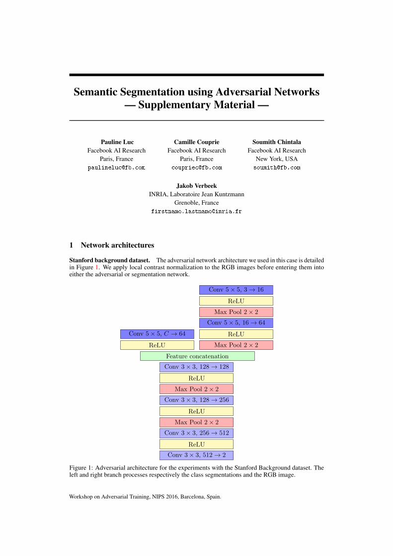
Stanford background dataset. The adversarial network architecture we used in this case is detailedin Figure 1. We apply local contrast normalization to the RGB images before entering them intoeither the adversarial or segmentation network.

Conv 5 ⇥ 5, C ! 64

ReLU

Conv 5 ⇥ 5, 3 ! 16

ReLU

Max Pool 2 ⇥ 2

Conv 5 ⇥ 5, 16 ! 64

ReLU

Max Pool 2 ⇥ 2

Feature concatenation

Conv 3 ⇥ 3, 128 ! 128

ReLU

Max Pool 2 ⇥ 2

Conv 3 ⇥ 3, 128 ! 256

ReLU

Max Pool 2 ⇥ 2

Conv 3 ⇥ 3, 256 ! 512

ReLU

Conv 3 ⇥ 3, 512 ! 2

Figure 1: Adversarial architecture for the experiments with the Stanford Background dataset. Theleft and right branch processes respectively the class segmentations and the RGB image.

Workshop on Adversarial Training, NIPS 2016, Barcelona, Spain.

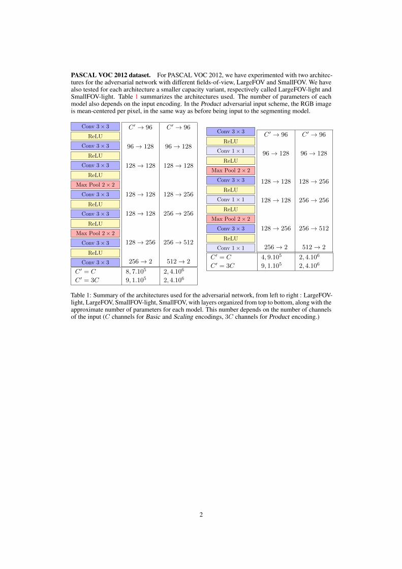
PASCAL VOC 2012 dataset. For PASCAL VOC 2012, we have experimented with two architec-tures for the adversarial network with different fields-of-view, LargeFOV and SmallFOV. We havealso tested for each architecture a smaller capacity variant, respectively called LargeFOV-light andSmallFOV-light. Table 1 summarizes the architectures used. The number of parameters of eachmodel also depends on the input encoding. In the Product adversarial input scheme, the RGB imageis mean-centered per pixel, in the same way as before being input to the segmenting model.

Conv 3 ⇥ 3

ReLU

Conv 3 ⇥ 3

ReLU

Conv 3 ⇥ 3

ReLU

Max Pool 2 ⇥ 2

Conv 3 ⇥ 3

ReLU

Conv 3 ⇥ 3

ReLU

Max Pool 2 ⇥ 2

Conv 3 ⇥ 3

ReLU

Conv 3 ⇥ 3

C 0 ! 96 C 0 ! 96

96 ! 128 96 ! 128

128 ! 128 128 ! 128

128 ! 128 128 ! 256

128 ! 128 256 ! 256

128 ! 256 256 ! 512

256 ! 2 512 ! 2

C 0 = C 8, 7.105 2, 4.106

C 0 = 3C 9, 1.105 2, 4.106

Conv 3 ⇥ 3

ReLU

Conv 1 ⇥ 1

ReLU

Max Pool 2 ⇥ 2

Conv 3 ⇥ 3

ReLU

Conv 1 ⇥ 1

ReLU

Max Pool 2 ⇥ 2

Conv 3 ⇥ 3

ReLU

Conv 1 ⇥ 1

C 0 ! 96 C 0 ! 96

96 ! 128 96 ! 128

128 ! 128 128 ! 256

128 ! 128 256 ! 256

128 ! 256 256 ! 512

256 ! 2 512 ! 2

C 0 = C 4, 9.105 2, 4.106

C 0 = 3C 9, 1.105 2, 4.106

Table 1: Summary of the architectures used for the adversarial network, from left to right : LargeFOV-light, LargeFOV, SmallFOV-light, SmallFOV, with layers organized from top to bottom, along with theapproximate number of parameters for each model. This number depends on the number of channelsof the input (C channels for Basic and Scaling encodings, 3C channels for Product encoding.)

2

2 Additional results

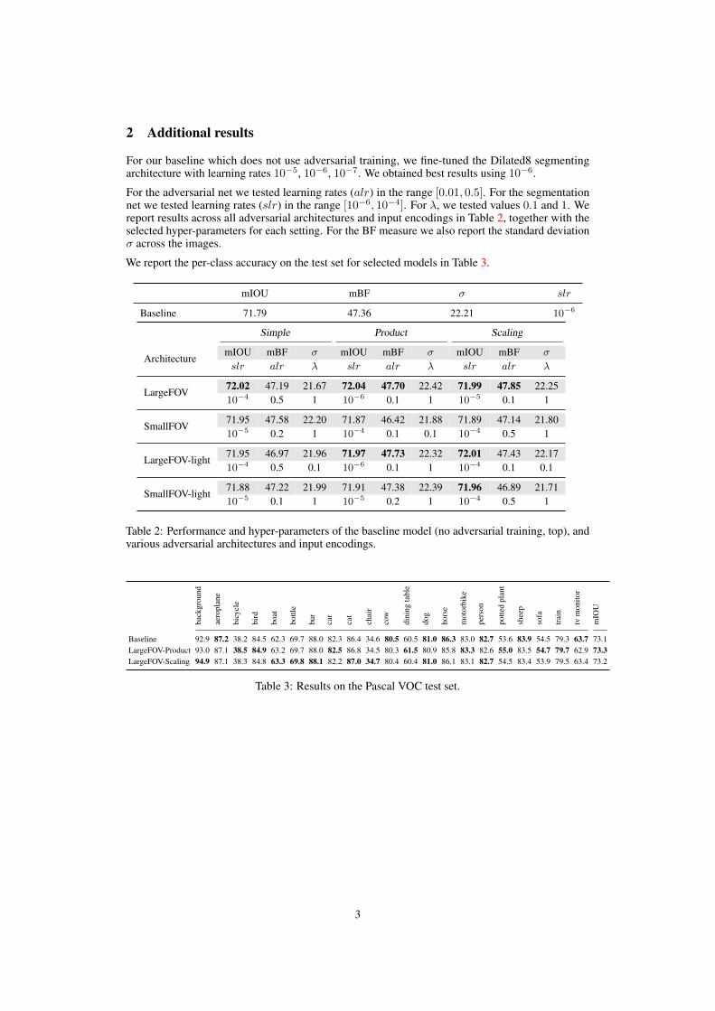
For our baseline which does not use adversarial training, we fine-tuned the Dilated8 segmentingarchitecture with learning rates 10�5, 10�6, 10�7. We obtained best results using 10�6.

For the adversarial net we tested learning rates (alr) in the range [0.01, 0.5]. For the segmentationnet we tested learning rates (slr) in the range [10�6, 10�4]. For �, we tested values 0.1 and 1. Wereport results across all adversarial architectures and input encodings in Table 2, together with theselected hyper-parameters for each setting. For the BF measure we also report the standard deviation� across the images.

We report the per-class accuracy on the test set for selected models in Table 3.

mIOU mBF � slr

Baseline 71.79 47.36 22.21 10�6

Simple Product Scaling

mIOU mBF � mIOU mBF � mIOU mBF �Architecture

slr alr � slr alr � slr alr �

72.02 47.19 21.67 72.04 47.70 22.42 71.99 47.85 22.25LargeFOV

10�4 0.5 1 10�6 0.1 1 10�5 0.1 1

71.95 47.58 22.20 71.87 46.42 21.88 71.89 47.14 21.80SmallFOV

10�5 0.2 1 10�4 0.1 0.1 10�4 0.5 1

71.95 46.97 21.96 71.97 47.73 22.32 72.01 47.43 22.17LargeFOV-light

10�4 0.5 0.1 10�6 0.1 1 10�4 0.1 0.1

71.88 47.22 21.99 71.91 47.38 22.39 71.96 46.89 21.71SmallFOV-light

10�5 0.1 1 10�5 0.2 1 10�4 0.5 1

Table 2: Performance and hyper-parameters of the baseline model (no adversarial training, top), andvarious adversarial architectures and input encodings.

back

grou

nd

aero

plan

e

bicy

cle

bird

boat

bottl

e

bur

car

cat

chai

r

cow

dini

ngta

ble

dog

hors

e

mot

orbi

ke

pers

on

potte

dpl

ant

shee

p

sofa

trai

n

tvm

onito

r

mIO

U

Baseline 92.9 87.2 38.2 84.5 62.3 69.7 88.0 82.3 86.4 34.6 80.5 60.5 81.0 86.3 83.0 82.7 53.6 83.9 54.5 79.3 63.7 73.1LargeFOV-Product 93.0 87.1 38.5 84.9 63.2 69.7 88.0 82.5 86.8 34.5 80.3 61.5 80.9 85.8 83.3 82.6 55.0 83.5 54.7 79.7 62.9 73.3LargeFOV-Scaling 94.9 87.1 38.3 84.8 63.3 69.8 88.1 82.2 87.0 34.7 80.4 60.4 81.0 86.1 83.1 82.7 54.5 83.4 53.9 79.5 63.4 73.2

Table 3: Results on the Pascal VOC test set.

3