Semi-Supervised Deep Ensembles for Blind Image Quality Assessment

Zhihua Wang1∗ , Dingquan Li2 , Kede Ma1

1Department of Computer Science, City University of Hong Kong2 Peng Cheng Laboratory

zhihua.wang@my.cityu,edu.hk, lidq01@pcl.ac.cn, kede.ma@cityu.edu.hk

AbstractEnsemble methods are generally regarded to bebetter than a single model if the base learners aredeemed to be “accurate” and “diverse.” Here weinvestigate a semi-supervised ensemble learningmethod to produce generalizable blind image qualityassessment models. We train a multi-head convolu-tional network for quality prediction by maximizingthe accuracy of the ensemble (as well as the baselearners) on labeled data, and the disagreement (i.e.,diversity) among them on unlabeled data, both im-plemented by the fidelity loss. We conduct exten-sive experiments to demonstrate the advantages ofemploying unlabeled data for BIQA, especially inmodel generalization and failure identification.

1 IntroductionData-driven blind image quality assessment (BIQA) mod-els [Bosse et al., 2018; Ma et al., 2018] employing deepconvolutional networks (ConvNets) have achieved unprece-dented performance, as measured by the correlations withhuman perceptual scores. However, the performance improve-ment may be doubtful due to the conflict between the smallscale of test IQA datasets and the large scale of ConvNetparameters, heightening the danger of poor generalizability.Ensemble learning, which aims to improve model general-izability by making use of multiple “accurate” and “diverse”base learners [Zhang and Ma, 2012], is a promising way ofalleviating this conflict, and has great potentials in outputtinggeneralizable BIQA models.

Researchers in the field of machine learning have con-tributed many brilliant ideas to ensemble learning, e.g., bag-ging [Breiman, 1996], boosting [Freund and Schapire, 1997],and negative correlation learning [Liu and Yao, 1999]. Thesemethods are mainly demonstrated under the supervised learn-ing setting where the training labels are given. In many real-world problems, plenty of unlabeled data are mostly freely ac-cessible, while the collection of human labels is prohibitivelylabor-expensive. For example, in BIQA, acquiring the meanopinion score (MOS) of one image involves effort of 15 to 30subjects [Sheikh et al., 2006].

∗Contact Author

In this paper, we combine labeled and unlabeled data totrain deep ensembles for BIQA in the semi-supervised set-ting [Chapelle et al., 2006; Chen et al., 2018]. Our methodis based on a multi-head ConvNet, where each head corre-sponds to a base learner and produces a quality estimate. Toreduce model complexity, the base learners share consider-able amount of early-stage computation and have separatelater-stage convolution and fully connected (FC) layers [Leeet al., 2015]. The ensemble is end-to-end optimized to tradeoff two theoretical conflicting objectives - ensemble accuracy(on labeled data) and diversity (on unlabeled data), both im-plemented through the fidelity loss [Tsai et al., 2007]. Weconduct extensive experiments to show that the learned en-semble performs favorably against a “top-performing” BIQAmodel - UNIQUE [Zhang et al., 2021b] in terms of qualityprediction on existing IQA datasets, while exhibiting muchstronger generalizability in the group maximum differentiation(gMAD) competition [Ma et al., 2020]. Moreover, our resultsfurther suggest that promoting diversity helps the ensemblespot its corner-case failures, which is in turn beneficial forsubsequent active learning [Wang and Ma, 2021].

2 MethodLet f (i) denotes the i-th base learner, which is implemented bya deep ConvNet, consisting of several stages of convolution,batch normalization [Ioffe and Szegedy, 2015], half-waverectification (i.e., ReLU nonlinearity) and spatial subsampling,followed by FC layers for quality computation. Given an inputimage x, the ensemble method f is simply defined by theaverage of all base learners:

f(x) =1

M

M∑i=1

f (i)(x), (1)

where M is the number of base learners used to build theensemble. A necessary condition for Eq. (1) to be valid isthat all base learners need to produce quality estimates of thesame perceptual scale, which is nontrivial to satisfy whenformulating BIQA as a ranking problem [Ma et al., 2017].We will give a detailed treatment of this scale alignment inSec. 2.1.

2.1 Supervised Ensemble Learning for BIQAFollowing [Ma et al., 2017; Zhang et al., 2021b], we choosethe pairwise learning-to-rank (L2R) method for BIQA learning

arX

iv:2

106.

1400

8v2

[cs

.CV

] 2

9 Ju

n 20

21

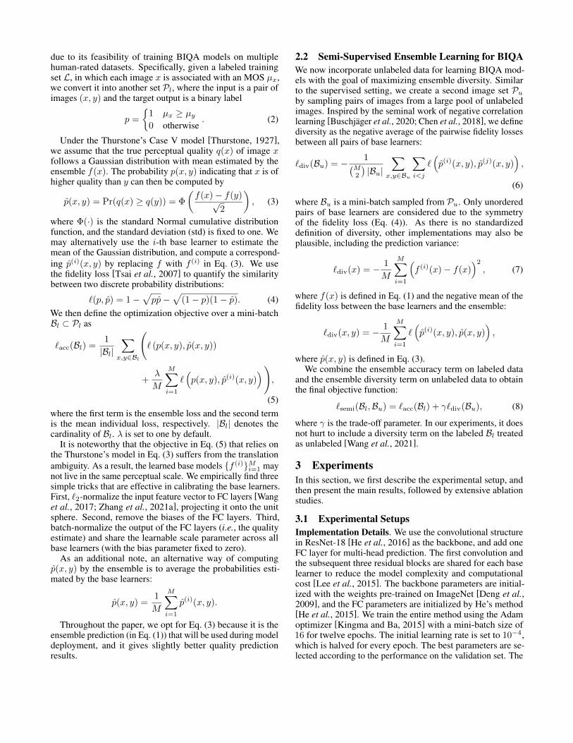
due to its feasibility of training BIQA models on multiplehuman-rated datasets. Specifically, given a labeled trainingset L, in which each image x is associated with an MOS µx,we convert it into another set Pl, where the input is a pair ofimages (x, y) and the target output is a binary label

p =

{1 µx ≥ µy

0 otherwise. (2)

Under the Thurstone’s Case V model [Thurstone, 1927],we assume that the true perceptual quality q(x) of image xfollows a Gaussian distribution with mean estimated by theensemble f(x). The probability p(x, y) indicating that x is ofhigher quality than y can then be computed by

p(x, y) = Pr(q(x) ≥ q(y)) = Φ

(f(x)− f(y)√

2

), (3)

where Φ(·) is the standard Normal cumulative distributionfunction, and the standard deviation (std) is fixed to one. Wemay alternatively use the i-th base learner to estimate themean of the Gaussian distribution, and compute a correspond-ing p(i)(x, y) by replacing f with f (i) in Eq. (3). We usethe fidelity loss [Tsai et al., 2007] to quantify the similaritybetween two discrete probability distributions:

`(p, p) = 1−√pp−

√(1− p)(1− p). (4)

We then define the optimization objective over a mini-batchBl ⊂ Pl as

`acc(Bl) =1

|Bl|∑

x,y∈Bl

(` (p(x, y), p(x, y))

+λ

M

M∑i=1

`(p(x, y), p(i)(x, y)

)),

(5)where the first term is the ensemble loss and the second termis the mean individual loss, respectively. |Bl| denotes thecardinality of Bl. λ is set to one by default.

It is noteworthy that the objective in Eq. (5) that relies onthe Thurstone’s model in Eq. (3) suffers from the translationambiguity. As a result, the learned base models {f (i)}Mi=1 maynot live in the same perceptual scale. We empirically find threesimple tricks that are effective in calibrating the base learners.First, `2-normalize the input feature vector to FC layers [Wanget al., 2017; Zhang et al., 2021a], projecting it onto the unitsphere. Second, remove the biases of the FC layers. Third,batch-normalize the output of the FC layers (i.e., the qualityestimate) and share the learnable scale parameter across allbase learners (with the bias parameter fixed to zero).

As an additional note, an alternative way of computingp(x, y) by the ensemble is to average the probabilities esti-mated by the base learners:

p(x, y) =1

M

M∑i=1

p(i)(x, y).

Throughout the paper, we opt for Eq. (3) because it is theensemble prediction (in Eq. (1)) that will be used during modeldeployment, and it gives slightly better quality predictionresults.

2.2 Semi-Supervised Ensemble Learning for BIQAWe now incorporate unlabeled data for learning BIQA mod-els with the goal of maximizing ensemble diversity. Similarto the supervised setting, we create a second image set Pu

by sampling pairs of images from a large pool of unlabeledimages. Inspired by the seminal work of negative correlationlearning [Buschjager et al., 2020; Chen et al., 2018], we definediversity as the negative average of the pairwise fidelity lossesbetween all pairs of base learners:

`div(Bu) = − 1(M2

)|Bu|

∑x,y∈Bu

∑i<j

`(p(i)(x, y), p(j)(x, y)

),

(6)

where Bu is a mini-batch sampled from Pu. Only unorderedpairs of base learners are considered due to the symmetryof the fidelity loss (Eq. (4)). As there is no standardizeddefinition of diversity, other implementations may also beplausible, including the prediction variance:

`div(x) = − 1

M

M∑i=1

(f (i)(x)− f(x)

)2, (7)

where f(x) is defined in Eq. (1) and the negative mean of thefidelity loss between the base learners and the ensemble:

`div(x, y) = − 1

M

M∑i=1

`(p(i)(x, y), p(x, y)

),

where p(x, y) is defined in Eq. (3).We combine the ensemble accuracy term on labeled data

and the ensemble diversity term on unlabeled data to obtainthe final objective function:

`semi(Bl,Bu) = `acc(Bl) + γ`div(Bu), (8)

where γ is the trade-off parameter. In our experiments, it doesnot hurt to include a diversity term on the labeled Bl treatedas unlabeled [Wang et al., 2021].

3 ExperimentsIn this section, we first describe the experimental setup, andthen present the main results, followed by extensive ablationstudies.

3.1 Experimental SetupsImplementation Details. We use the convolutional structurein ResNet-18 [He et al., 2016] as the backbone, and add oneFC layer for multi-head prediction. The first convolution andthe subsequent three residual blocks are shared for each baselearner to reduce the model complexity and computationalcost [Lee et al., 2015]. The backbone parameters are initial-ized with the weights pre-trained on ImageNet [Deng et al.,2009], and the FC parameters are initialized by He’s method[He et al., 2015]. We train the entire method using the Adamoptimizer [Kingma and Ba, 2015] with a mini-batch size of16 for twelve epochs. The initial learning rate is set to 10−4,which is halved for every epoch. The best parameters are se-lected according to the performance on the validation set. The

Best SSL Ensemble

Worst SSL Ensemble

Fixed UNIQUE

(a) Top: 72, bottom: 48

Best SSL Ensemble

Worst SSL Ensemble

Fixed UNIQUE

(b) Top: 72, bottom: 23

Best UNIQUE

Worst UNIQUE

Fixed SSL Ensemble

(c) Top: 62, bottom: 70

Best UNIQUE

Worst UNIQUE

Fixed SSLEnsemble

(d) Top: 72, bottom: 74

Figure 1: Representative gMAD pairs between UNIQUE [Zhang et al., 2021b] and the SSL ensemble on FLIVE [Ying et al., 2020]. Shown inthe sub-caption is the MOS of each image. (a) Fixing UNIQUE at the low-quality level. (b) Fixing UNIQUE at the high-quality level. (c)Fixing the SSL ensemble at the low-quality level. (d) Fixing the SSL ensemble at the high-quality level.

Table 1: Correlation between model predictions and MOSs on thetest sets of KonIQ-10k [Hosu et al., 2020], SPAQ [Fang et al., 2020],and FLIVE [Ying et al., 2020], respectively.

SRCC KonIQ-10k SPAQ FLIVEUNIQUE 0.860 0.899 0.426Naıve Ensemble 0.855 0.900 0.427Joint Ensemble 0.864 0.899 0.430SSL Ensemble 0.861 0.900 0.438

PLCC KonIQ-10k SPAQ FLIVEUNIQUE 0.859 0.904 0.505Naıve Ensemble 0.859 0.903 0.517Joint Ensemble 0.870 0.903 0.521SSL Ensemble 0.861 0.904 0.527

images during training are cropped to 384×384, keeping theiraspect ratios, while the test images are fed with the originalsizes.Datasets. We use 60% images in KonIQ-10k [Hosu et al.,2020] and SPAQ [Fang et al., 2020] as the labeled training set,20% as the validation set, and 20% as the test set, respectively.We treat the entire FLIVE [Ying et al., 2020] as the unlabeledtraining set. To reduce the bias caused by the random splitting,we repeat the procedure three times, and report the meanresults.Evaluation Metrics. We adopt two quantitative criteria:Spearman rank-order correlation coefficient (SRCC) and Pear-son linear correlation coefficient (PLCC), to measure predic-tion performance, respectively. Before computing PLCC, afour-parameter logistic function is suggested in [VQEG, 2000]to fit model predictions to subjective scores:

f(x) = (η1 − η2)/(1 + exp(−(f(x)− η3)/|η4|)) + η2,(9)

Table 2: Comparison of the failure-spotting efficiency as a functionof the number of selected samples on FLIVE [Ying et al., 2020]. Alower correlation coefficient indicates better performance.

SRCC 500 1, 000 1, 500 2, 000UNIQUE 0.358 0.373 0.352 0.377Naıve Ensemble 0.458 0.397 0.391 0.384Joint Ensemble 0.346 0.355 0.360 0.370SSL Ensemble 0.338 0.305 0.318 0.326

PLCC 500 1, 000 1, 500 2, 000UNIQUE 0.463 0.460 0.456 0.483Naıve Ensemble 0.504 0.461 0.452 0.441Joint Ensemble 0.483 0.483 0.488 0.482SSL Ensemble 0.378 0.384 0.390 0.400

where {ηi; i = 1, 2, 3, 4} are the parameters to be optimized.

3.2 Main ResultsCorrelation Results. We compare our method (termed as theSSL ensemble) against three variants: 1) UNIQUE [Zhanget al., 2021b], a state-of-the-art BIQA model, correspondingto M = 1; 2) Naıve Ensemble, corresponding to λ = 0 inEq. (5) and γ = 0 in Eq. (8); 3) Joint Ensemble, correspondingto γ = 0. The mean SRCC and PLCC results are listedin Table 1, where we find that the SSL ensemble performsfavorably against the competing methods.gMAD Results. We next let the SSL ensemble play thegMAD competition game [Ma et al., 2020] with UNIQUEon the FLIVE database. Figure 1 shows the representativegMAD pairs. It is clear that the pairs of images in (a) and(b), where UNIQUE and the SSL ensemble perform the de-fender and attacker roles, respectively, exhibit substantiallydifferent quality, which is in disagreement with UNIQUE. Incontrast, the SSL ensemble correctly predicts the top images

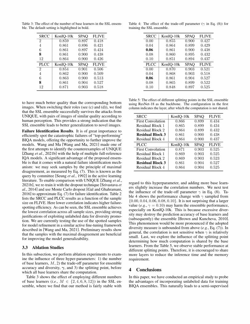
Table 3: The effect of the number of base learners in the SSL ensem-ble. The default setting is highlighted in bold.

SRCC KonIQ-10k SPAQ FLIVE2 0.859 0.897 0.4184 0.861 0.896 0.4216 0.861 0.897 0.4248 0.861 0.900 0.43812 0.864 0.900 0.426

PLCC KonIQ-10k SPAQ FLIVE2 0.854 0.901 0.5064 0.862 0.900 0.5096 0.863 0.900 0.5138 0.861 0.904 0.52712 0.871 0.903 0.518

to have much better quality than the corresponding bottomimages. When switching their roles (see (c) and (d)), we findthat the SSL ensemble successfully survives the attacks fromUNIQUE, with pairs of images of similar quality according tohuman perception. This provides a strong indication that theSSL ensemble leads to better generalization to novel images.Failure Identification Results. It is of great importance toefficiently spot the catastrophic failures of “top-performing”BIQA models, offering the opportunity to further improve themodels. Wang and Ma [Wang and Ma, 2021] made one ofthe first attempts to identify the counterexamples of UNIQUE[Zhang et al., 2021b] with the help of multiple full-referenceIQA models. A significant advantage of the proposed ensem-ble is that it comes with a natural failure identification mech-anism: we may seek samples by the principle of maximaldisagreement, as measured by Eq. (7). This is known as thequery by committee [Seung et al., 1992] in the active learningliterature. To enable comparison with UNIQUE [Zhang et al.,2021b], we re-train it with the dropout technique [Srivastava etal., 2014] and use Monte Carlo dropout [Gal and Ghahramani,2016] to approximate Eq. (7) for failure identification. Table 2lists the SRCC and PLCC results as a function of the samplesize on FLIVE. Here lower correlation indicates higher failure-spotting efficiency. As can be seen, the SSL ensemble achievesthe lowest correlation across all sample sizes, providing strongjustifications of exploiting unlabeled data for diversity promo-tion. We are currently testing the use of the spotted samplesfor model refinement in a similar active fine-tuning frameworkdescribed in [Wang and Ma, 2021]. Preliminary results showthat the samples with the maximal disagreement are beneficialfor improving the model generalizability.

3.3 Ablation StudiesIn this subsection, we perform ablation experiments to exam-ine the influence of three hyper-parameters: 1) the numberof base learners, M , 2) the trade-off parameter for ensembleaccuracy and diversity, γ, and 3) the splitting point, beforewhich all base learners share the computation.

Table 3 shows the effect of employing different numbersof base learners (i.e., M ∈ {2, 4, 6, 8, 12}) in the SSL en-semble, where we find that our method is fairly stable with

Table 4: The effect of the trade-off parameter (γ in Eq. (8)) fortraining the SSL ensemble.

SRCC KonIQ-10k SPAQ FLIVE0.00 0.855 0.900 0.4270.04 0.864 0.899 0.4290.06 0.861 0.900 0.4380.08 0.860 0.895 0.4320.10 0.851 0.894 0.437

PLCC KonIQ-10k SPAQ FLIVE0.00 0.870 0.903 0.5210.04 0.868 0.903 0.5180.06 0.861 0.904 0.5270.08 0.865 0.899 0.5220.10 0.848 0.897 0.525

Table 5: The effect of different splitting points in the SSL ensembleusing ResNet-18 as the backbone. The configuration in the firstcolumn indicates the layer, after which the computation is not shared.

SRCC KonIQ-10k SPAQ FLIVEFirst Convolution 0.866 0.899 0.434Residual Block 1 0.865 0.899 0.434Residual Block 2 0.864 0.899 0.432Residual Block 3 0.861 0.900 0.438Residual Block 4 0.864 0.900 0.437

PLCC KonIQ-10k SPAQ FLIVEFirst Convolution 0.871 0.903 0.525Residual Block 1 0.869 0.903 0.525Residual Block 2 0.869 0.903 0.523Residual Block 3 0.861 0.904 0.527Residual Block 4 0.864 0.904 0.525

regard to this hyperparameter, and adding more base learn-ers slightly increase the correlation numbers. We next testthe influence of the trade-off parameter γ in Eq. (8). Ta-ble 4 shows the performance change with γ sampled from{0.00, 0.04, 0.06, 0.08, 0.10}. It is not surprising that a largervalue (e.g., γ = 0.10) may harm the ensemble performance,especially on KonIQ-10k. This is because excessive diver-sity may destroy the prediction accuracy of base learners and(subsequently) the ensemble [Brown and Kuncheva, 2010].This phenomenon would be more pronounced if the adopteddiversity measure is unbounded from above (e.g., Eq. (7)). Ingeneral, the correlation is not sensitive when γ is relativelysmall. Last, we explore the influence of the splitting pointdetermining how much computation is shared by the baselearners. From the Table 5, we observe stable performance atdifferent splitting points. Therefore, it is encouraged to sharemore layers to reduce the inference time and the memoryrequirement.

4 ConclusionsIn this paper, we have conducted an empirical study to probethe advantages of incorporating unlabeled data for trainingBIQA ensembles. This naturally leads to a semi-supervised

formulation, where we maximized the ensemble accuracy onlabeled data and the ensemble diversity on unlabeled data.Through comprehensive experiments, we arrived at three in-teresting findings. First, the diversity-driven SSL ensembledoes not achieve correlation improvements on existing IQAdatabases. Second, despite similar correlation performance,our ensemble shows much stronger generalizability in thegMAD competition with greater potentials for use in monitor-ing real-world quality problems. Third, our ensemble has abuilt-in failure-identification mechanism with demonstratedefficiency. This points to an interesting avenue for futurework - active fine-tuning BIQA models in the semi-supervisedsetting.

References[Bosse et al., 2018] S. Bosse, D. Maniry, K.-R. Muller,

T. Wiegand, and W. Samek. Deep neural networks forno-reference and full-reference image quality assessment.IEEE Transactions on Image Processing, 27(1):206–219,2018.

[Breiman, 1996] L. Breiman. Bagging predictors. MachineLearning, 24(2):123–140, 1996.

[Brown and Kuncheva, 2010] G. Brown and L. I. Kuncheva.“good” and “bad” diversity in majority vote ensembles.In International Workshop on Multiple Classifier Systems,pages 124–133, 2010.

[Buschjager et al., 2020] S. Buschjager, L. Pfahler, andK. Morik. Generalized negative correlation learning fordeep ensembling. arXiv preprint arXiv:2011.02952, 2020.

[Chapelle et al., 2006] O. Chapelle, B. Scholkopf, andA. Zien, editors. Semi-Supervised Learning. The MITPress, 2006.

[Chen et al., 2018] H. Chen, B. Jiang, and X. Yao. Semisu-pervised negative correlation learning. IEEE Transactionson Neural Networks and Learning Systems, 29(11):5366–5379, 2018.

[Deng et al., 2009] J. Deng, W. Dong, R. Socher, L.-J. Li,K. Li, and L. Fei-Fei. ImageNet: A large-scale hierarchicalimage database. In IEEE Conference on Computer Visionand Pattern Recognition, pages 248–255, 2009.

[Fang et al., 2020] Y. Fang, H. Zhu, Y. Zeng, K. Ma, andZ. Wang. Perceptual quality assessment of smartphonephotography. In IEEE Conference on Computer Vision andPattern Recognition, pages 3677–3686, 2020.

[Freund and Schapire, 1997] Y. Freund and R. E. Schapire. Adecision-theoretic generalization of on-line learning and anapplication to boosting. Journal of Computer and SystemSciences, 55(1):119–139, 1997.

[Gal and Ghahramani, 2016] Y. Gal and Z. Ghahramani.Dropout as a Bayesian approximation: Representing modeluncertainty in deep learning. In International Conferenceon Machine Learning, pages 1050–1059, 2016.

[He et al., 2015] K. He, X. Zhang, S. Ren, and J. Sun. Delv-ing deep into rectifiers: Surpassing human-level perfor-mance on ImageNet classification. In IEEE InternationalConference on Computer Vision, pages 1026–1034, 2015.

[He et al., 2016] K. He, X. Zhang, S. Ren, and J. Sun. Deepresidual learning for image recognition. In IEEE Confer-ence on Computer Vision and Pattern Recognition, pages770–778, 2016.

[Hosu et al., 2020] V. Hosu, H. Lin, T. Sziranyi, and D. Saupe.KonIQ-10k: An ecologically valid database for deep learn-ing of blind image quality assessment. IEEE Transactionson Image Processing, 29:4041–4056, 2020.

[Ioffe and Szegedy, 2015] S. Ioffe and C. Szegedy. Batchnormalization: Accelerating deep network training by re-ducing internal covariate shift. In International Conferenceon Machine Learning, page 448–456, 2015.

[Kingma and Ba, 2015] D. P. Kingma and J. Ba. Adam: Amethod for stochastic optimization. In International Con-ference on Learning Representations, 2015.

[Lee et al., 2015] S. Lee, S. Purushwalkam, M. Cogswell,D. Crandall, and D. Batra. Why M heads are better thanone: Training a diverse ensemble of deep networks. arXivpreprint arXiv:1511.06314, 2015.

[Liu and Yao, 1999] Y. Liu and X. Yao. Ensemble learningvia negative correlation. Neural Networks, 12(10):1399–1404, 1999.

[Ma et al., 2017] K. Ma, W. Liu, T. Liu, Z. Wang, and D. Tao.dipIQ: Blind image quality assessment by learning-to-rankdiscriminable image pairs. IEEE Transactions on ImageProcessing, 26(8):3951–3964, 2017.

[Ma et al., 2018] K. Ma, W. Liu, K. Zhang, Z. Duanmu,Z. Wang, and W. Zuo. End-to-end blind image qualityassessment using deep neural networks. IEEE Transactionson Image Processing, 27(3):1202–1213, 2018.

[Ma et al., 2020] K. Ma, Z. Duanmu, Z. Wang, Q. Wu,W. Liu, H. Yong, H. Li, and L. Zhang. Group maximumdifferentiation competition: Model comparison with fewsamples. IEEE Transactions on Pattern Analysis and Ma-chine Intelligence, 42(4):851–864, 2020.

[Seung et al., 1992] H. S. Seung, M. Opper, and H. Sompolin-sky. Query by committee. In Annual Workshop on Compu-tational Learning Theory, pages 287–294, 1992.

[Sheikh et al., 2006] H. R. Sheikh, M. F. Sabir, and A. C.Bovik. A statistical evaluation of recent full referenceimage quality assessment algorithms. IEEE Transactionson Image Processing, 15(11):3440–3451, 2006.

[Srivastava et al., 2014] N. Srivastava, G. Hinton,A. Krizhevsky, I. Sutskever, and R. Salakhutdinov.Dropout: A simple way to prevent neural networks fromoverfitting. Journal of Machine Learning Research,15(1):1929–1958, 2014.

[Thurstone, 1927] L. L. Thurstone. A law of comparativejudgment. Psychological Review, 34(4):273–286, 1927.

[Tsai et al., 2007] M.-F. Tsai, T.-Y. Liu, T. Qin, H.-H. Chen,and W.-Y. Ma. FRank: A ranking method with fidelity loss.In ACM SIGIR Conference on Research and Developmentin Information Retrieval, pages 383–390, 2007.

[VQEG, 2000] VQEG. Final report from the Video QualityExperts Group on the validation of objective models ofvideo quality assessment, 2000.

[Wang and Ma, 2021] Z. Wang and K. Ma. Active fine-tuningfrom gMAD examples improves blind image quality assess-ment. IEEE Transactions on Pattern Analysis and MachineIntelligence, 2021.

[Wang et al., 2017] F. Wang, X. Xiang, J. Cheng, and A. L.Yuille. NormFace: L2 hypersphere embedding for face ver-ification. In ACM International Conference on Multimedia,pages 1041–1049, 2017.

[Wang et al., 2021] X. Wang, L. Lian, Z. Miao, Z. Liu,and S. Yu. Long-tailed recognition by routing diversedistribution-aware experts. In International Conferenceon Learning Representations, 2021.

[Ying et al., 2020] Z. Ying, H. Niu, P. Gupta, D. Mahajan,D. Ghadiyaram, and A. Bovik. From patches to pictures(PaQ-2-PiQ): Mapping the perceptual space of picture qual-ity. In IEEE Conference on Computer Vision and PatternRecognition, pages 3575–3585, 2020.

[Zhang and Ma, 2012] C. Zhang and Y. Ma, editors. En-semble Machine Learning: Methods and Applications.Springer, 2012.

[Zhang et al., 2021a] W. Zhang, D. Li, C. Ma, G. Zhai,X. Yang, and K. Ma. Continual learning for blind im-age quality assessment. arXiv preprint arXiv:2102.09717,2021.

[Zhang et al., 2021b] W. Zhang, K. Ma, G. Zhai, and X. Yang.Uncertainty-aware blind image quality assessment in thelaboratory and wild. IEEE Transactions on Image Process-ing, 30:3474–3486, 2021.