semi-supervised learning for natural languagecs.stanford.edu/~pliang/papers/meng-thesis.pdf ·...
TRANSCRIPT

Semi-Supervised Learning for Natural Language
by
Percy Liang
Submitted to the Department of Electrical Engineering and ComputerScience
in partial fulfillment of the requirements for the degree of
Master of Engineering in Electrical Engineering and Computer Science
at the
MASSACHUSETTS INSTITUTE OF TECHNOLOGY
May 2005
c© Massachusetts Institute of Technology 2005. All rights reserved.
Author . . . . . . . . . . . . . . . . . . . . . . . . . . . . . . . . . . . . . . . . . . . . . . . . . . . . . . . . . . . . . .Department of Electrical Engineering and Computer Science
May 19, 2005
Certified by. . . . . . . . . . . . . . . . . . . . . . . . . . . . . . . . . . . . . . . . . . . . . . . . . . . . . . . . . .
Michael CollinsAssistant Professor, CSAIL
Thesis Supervisor
Accepted by . . . . . . . . . . . . . . . . . . . . . . . . . . . . . . . . . . . . . . . . . . . . . . . . . . . . . . . . .Arthur C. Smith
Chairman, Department Committee on Graduate Students

2

Semi-Supervised Learning for Natural Language
by
Percy Liang
Submitted to the Department of Electrical Engineering and Computer Scienceon May 19, 2005, in partial fulfillment of the
requirements for the degree ofMaster of Engineering in Electrical Engineering and Computer Science
Abstract
Statistical supervised learning techniques have been successful for many natural lan-guage processing tasks, but they require labeled datasets, which can be expensive toobtain. On the other hand, unlabeled data (raw text) is often available “for free” inlarge quantities. Unlabeled data has shown promise in improving the performanceof a number of tasks, e.g. word sense disambiguation, information extraction, andnatural language parsing.
In this thesis, we focus on two segmentation tasks, named-entity recognition andChinese word segmentation. The goal of named-entity recognition is to detect andclassify names of people, organizations, and locations in a sentence. The goal ofChinese word segmentation is to find the word boundaries in a sentence that hasbeen written as a string of characters without spaces.
Our approach is as follows: In a preprocessing step, we use raw text to clusterwords and calculate mutual information statistics. The output of this step is thenused as features in a supervised model, specifically a global linear model trained usingthe Perceptron algorithm. We also compare Markov and semi-Markov models on thetwo segmentation tasks. Our results show that features derived from unlabeled datasubstantially improves performance, both in terms of reducing the amount of labeleddata needed to achieve a certain performance level and in terms of reducing the errorusing a fixed amount of labeled data. We find that sometimes semi-Markov modelscan also improve performance over Markov models.
Thesis Supervisor: Michael CollinsTitle: Assistant Professor, CSAIL
3

4

Acknowledgments
This work was done under the supervision of my advisor, Michael Collins. Since I
started working on my masters research, I have learned much about machine learning
and natural language processing from him, and I appreciate his guidance and en-
couragement. I would also like to thank my parents for their continual support and
Ashley Kim for editing this manuscript and helping me get through this process.
5

6

Contents
1 Introduction 13
2 The segmentation tasks 17
2.1 Chinese word segmentation (CWS) . . . . . . . . . . . . . . . . . . . 17
2.1.1 The task . . . . . . . . . . . . . . . . . . . . . . . . . . . . . . 17
2.1.2 What is a word? . . . . . . . . . . . . . . . . . . . . . . . . . 18
2.1.3 Datasets . . . . . . . . . . . . . . . . . . . . . . . . . . . . . . 19
2.1.4 Challenges . . . . . . . . . . . . . . . . . . . . . . . . . . . . . 20
2.1.5 Existing methods . . . . . . . . . . . . . . . . . . . . . . . . . 21
2.2 Named-entity recognition (NER) . . . . . . . . . . . . . . . . . . . . 22
2.2.1 The task . . . . . . . . . . . . . . . . . . . . . . . . . . . . . . 22
2.2.2 Datasets . . . . . . . . . . . . . . . . . . . . . . . . . . . . . . 23
2.2.3 Challenges . . . . . . . . . . . . . . . . . . . . . . . . . . . . . 23
2.2.4 Existing methods . . . . . . . . . . . . . . . . . . . . . . . . . 24
2.3 Evaluation . . . . . . . . . . . . . . . . . . . . . . . . . . . . . . . . . 26
3 Learning methods 29
3.1 The setup: classification . . . . . . . . . . . . . . . . . . . . . . . . . 29
3.2 Global linear models . . . . . . . . . . . . . . . . . . . . . . . . . . . 30
3.2.1 Definition . . . . . . . . . . . . . . . . . . . . . . . . . . . . . 30
3.2.2 Types of models . . . . . . . . . . . . . . . . . . . . . . . . . . 31
3.2.3 Decoding . . . . . . . . . . . . . . . . . . . . . . . . . . . . . 35
3.2.4 Training . . . . . . . . . . . . . . . . . . . . . . . . . . . . . . 37
7

3.2.5 Other parameter estimation algorithms . . . . . . . . . . . . . 38
3.3 Semi-supervised techniques . . . . . . . . . . . . . . . . . . . . . . . . 39
3.3.1 Generative maximum-likelihood models . . . . . . . . . . . . . 39
3.3.2 Co-training and bootstrapping . . . . . . . . . . . . . . . . . . 39
3.3.3 Partitioning . . . . . . . . . . . . . . . . . . . . . . . . . . . . 40
3.3.4 Using features derived from unlabeled data . . . . . . . . . . . 41
4 Extracting features from raw text 43
4.1 Word clustering . . . . . . . . . . . . . . . . . . . . . . . . . . . . . . 43
4.1.1 The Brown algorithm . . . . . . . . . . . . . . . . . . . . . . . 44
4.1.2 Extracting word clusters . . . . . . . . . . . . . . . . . . . . . 51
4.1.3 Utility of word clusters . . . . . . . . . . . . . . . . . . . . . . 51
4.2 Mutual information . . . . . . . . . . . . . . . . . . . . . . . . . . . . 52
4.2.1 Extracting mutual information . . . . . . . . . . . . . . . . . . 53
4.2.2 Utility of mutual information . . . . . . . . . . . . . . . . . . 53
4.3 Incorporating features from unlabeled data . . . . . . . . . . . . . . . 54
4.3.1 Using word cluster features . . . . . . . . . . . . . . . . . . . 54
4.3.2 Using mutual information features . . . . . . . . . . . . . . . . 55
5 Experiments 59
5.1 Features . . . . . . . . . . . . . . . . . . . . . . . . . . . . . . . . . . 59
5.2 Results . . . . . . . . . . . . . . . . . . . . . . . . . . . . . . . . . . . 64
5.2.1 Effect of using unlabeled data features . . . . . . . . . . . . . 66
5.2.2 Effect of using semi-Markov models . . . . . . . . . . . . . . . 68
5.2.3 Lexicon-based features . . . . . . . . . . . . . . . . . . . . . . 69
6 Conclusion 73
8

List of Figures
2-1 The goal of Chinese word segmentation is to find the word boundaries
in a string of Chinese characters. This example is from the Chinese
Treebank (Section 2.1.3). . . . . . . . . . . . . . . . . . . . . . . . . . 17
2-2 The translation of a Chinese sentence. . . . . . . . . . . . . . . . . . 18
2-3 The goal of named-entity recognition (NER) is to find the names of
various entities. The example is from the English dataset (Section 2.2.2). 23
3-1 An example of BIO tagging for named-entity recognition. . . . . . . . 32
3-2 The Averaged Perceptron algorithm. . . . . . . . . . . . . . . . . . . 37
4-1 The class-based bigram language model, which defines the quality of a
clustering, represented as a Bayesian network. . . . . . . . . . . . . . 44
4-2 Visualizing the Brown algorithm. (a) shows the edges involved in com-
puting L(c, c′) from scratch (solid indicates added, dashed indicates
subtracted). (b) shows the edges involved in computing ∆L(c, c′), the
change in L(c, c′) when the two nodes in the shaded box have just been
merged. . . . . . . . . . . . . . . . . . . . . . . . . . . . . . . . . . . 48
4-3 Examples of English word clusters. . . . . . . . . . . . . . . . . . . . 51
4-4 A histogram showing the distribution of mutual information values
estimated from unsegmented Chinese text. . . . . . . . . . . . . . . . 56
5-1 Markov model features for CWS. ti is the current tag, xi is the current
character, and MIz(xi−1, xi) is the mutual information z-score of the
previous and current characters. . . . . . . . . . . . . . . . . . . . . . 62
9

5-2 Semi-Markov model features for CWS. lj is the current segment label;
s and e are the starting and ending indices of the current segment,
respectively. . . . . . . . . . . . . . . . . . . . . . . . . . . . . . . . . 62
5-3 Markov model features for NER. C andM are sets of string operations. 63
5-4 Semi-Markov model features for NER. . . . . . . . . . . . . . . . . . 63
5-5 Test F1 performance on CTB . . . . . . . . . . . . . . . . . . . . . . 67
5-6 Test F1 performance on PK . . . . . . . . . . . . . . . . . . . . . . . 68
5-7 Test F1 performance on HK . . . . . . . . . . . . . . . . . . . . . . . 69
5-8 Test F1 performance on Eng . . . . . . . . . . . . . . . . . . . . . . . 70
5-9 Test F1 performance on Deu . . . . . . . . . . . . . . . . . . . . . . . 71
10

List of Tables
2.1 Statistics of three Chinese word segmentation datasets (CTB, PK, and
HK) from the First International Chinese Word Segmentation Bakeoff. 20
2.2 Statistics of the English (Eng) and German (Deu) named-entity recog-
nition datasets from the CoNLL 2003 Shared Task (Sang and Meulder,
2003). . . . . . . . . . . . . . . . . . . . . . . . . . . . . . . . . . . . 24
4.1 Mutual information values of various Chinese character pairs. . . . . 53
4.2 Mutual information across word boundaries is much lower than mutual
information within words. The test was done on the PK Train set. . . 54
4.3 F1 scores obtained by using various ways to transform mutual infor-
mation values before using them in a Markov model. The experiments
were done on the HK dataset. 10% of the total available training data
(29K characters) was used. . . . . . . . . . . . . . . . . . . . . . . . . 57
5.1 For each dataset (CTB, PK, etc.) and each of its three sets of examples
(Train, Dev, and Test), we show the bound on the segment length as
computed from the examples in that set, as well as the maximum
segment length. Note that only the bounds computed from the Train
set are used in training and testing. . . . . . . . . . . . . . . . . . . . 64
5.2 Results on the CTB (Test) dataset. . . . . . . . . . . . . . . . . . . . 65
5.3 Results on the PK (Test) dataset. . . . . . . . . . . . . . . . . . . . . 65
5.4 Results on the HK (Test) dataset. . . . . . . . . . . . . . . . . . . . . 65
5.5 Results on the Eng (Test) dataset. . . . . . . . . . . . . . . . . . . . 66
5.6 Results on the Deu (Test) dataset. . . . . . . . . . . . . . . . . . . . 66
11

5.7 Test F1 scores obtained by the M+F and SM+F models on Chinese
word segmentation. M+F and SM+F are the Markov and semi-Markov
models using mutual information features; CRF (closed and open)
refers to (Peng et al., 2004) using closed and open feature sets; and
CRF+HMMLDA refers to (Li and McCallum, 2005). . . . . . . . . . 67
5.8 Dev and Test F1 scores obtained by the M+F and SM+F models on
named-entity recognition. M+F and SM+F are the Markov and semi-
Markov models using word clustering features; CRF refers to (McCal-
lum and Li, 2003). . . . . . . . . . . . . . . . . . . . . . . . . . . . . 68
5.9 Experiments on using lexicon-based features for CWS on the CTB
dataset. . . . . . . . . . . . . . . . . . . . . . . . . . . . . . . . . . . 70
1 Improvements on Test F1 due to M → M+F. . . . . . . . . . . . . . 83
2 Reductions on the amount of labeled data due to M → M+F. Test F1
scores are achieved by M using 100% of the training data. Datasets for
which M performs better than M+F are marked n/a. . . . . . . . . . 83
3 Improvements on Test F1 due to SM → SM+F. . . . . . . . . . . . . 84
4 Reductions on the amount of labeled data due to SM → SM+F. Test
F1 scores are achieved by SM using 100% of the training data. Datasets
for which SM performs better than SM+F are marked n/a. . . . . . . 84
5 Improvements on Test F1 due to M → SM. . . . . . . . . . . . . . . . 85
6 Reductions on the amount of labeled data due to M → SM. Test F1
scores are achieved by M using 100% of the training data. Datasets for
which M performs better than SM are marked n/a. . . . . . . . . . . 85
7 Improvements on Test F1 due to M+F → SM+F. . . . . . . . . . . . 86
8 Reductions on the amount of labeled data due to M+F → SM+F.
Test F1 scores are achieved by M+F using 100% of the training data.
Datasets for which M+F performs better than SM+F are marked n/a. 86
12
Chapter 1
Introduction
In recent years, statistical learning methods have been highly successful for tackling
natural language tasks. Due to the increase in computational resources over the last
decade, it has been possible to apply these methods in large-scale natural language
experiments on real-world data such as newspaper articles. Such domains are chal-
lenging because they are complex and noisy, but statistical approaches have proven
robust in dealing with these issues.
Most of these successful machine learning algorithms are supervised, which means
that they require labeled data—examples of potential inputs paired with the corre-
sponding correct outputs. This labeled dataset must often be created by hand, which
can be time consuming and expensive. Moreover, a new labeled dataset must be cre-
ated for each new problem domain. For example, a supervised algorithm that learns
to detect company-location relations in text would require examples of (company,
location) pairs. The same algorithm could potentially learn to also detect country-
capital relations, but an entirely new dataset of (country, capital) pairs would be
required.
While labeled data is expensive to obtain, unlabeled data is essentially free in
comparison. It exists simply as raw text from sources such as the Internet. Only a
minimal amount of preprocessing (e.g., inserting spaces between words and punctu-
ation) is necessary to convert the raw text into unlabeled data suitable for use in an
unsupervised or semi-supervised learning algorithm. Previous work has shown that
13

using unlabeled data to complement a traditional labeled dataset can improve perfor-
mance (Miller et al., 2004; Abney, 2004; Riloff and Jones, 1999; Collins and Singer,
1999; Blum and Mitchell, 1998; Yarowsky, 1995). There are two ways of character-
izing performance gains due to using additional unlabeled data: (1) the reduction in
error using the same amount of labeled data and (2) the reduction in the amount of
labeled data needed to reach the same error threshold. In Chapter 5, we describe our
improvements using both criteria.
We consider using unlabeled data for segmentation tasks. These tasks involve
learning a mapping from an input sentence to an underlying segmentation. Many
NLP tasks (e.g., named-entity recognition, noun phrase chunking, and Chinese word
segmentation) can be cast into this framework. In this thesis, we focus on two
segmentation tasks: named-entity recognition and Chinese word segmentation. In
named-entity recognition, the goal is to identify names of the entities (e.g., people,
organizations, and locations) that occur in a sentence. In terms of segmentation,
the goal is to partition a sentence into segments, each of which corresponds either a
named-entity or a single-word non-entity. In addition, each entity segment is labeled
with its type (e.g., person, location, etc.). In Chinese word segmentation, the goal
is to partition a sentence, which is a string of characters written without delimiting
spaces, into words. See Chapter 2 for a full description of these two tasks.
In the spirit of (Miller et al., 2004), our basic strategy for taking advantage of
unlabeled data is to first derive features from unlabeled data—in our case, word
clustering or mutual information features—and then use these features in a supervised
learning algorithm. (Miller et al., 2004) achieved significant performance gains in
named-entity recognition by using word clustering features and active learning. In
this thesis, we show that another type of unlabeled data feature based on mutual
information can also significantly improve performance.
The supervised models that we use to incorporate unlabeled data features come
from the class of global linear models (Section 3.2). Global linear models (GLMs),
which include Conditional Random Fields (Lafferty et al., 2001a) and max-margin
Markov networks (Taskar et al., 2003), are discriminatively trained models for struc-
14

tured classification. They allow the flexibility of defining arbitrary features over an
entire sentence and a candidate segmentation. We consider two types of GLMs,
Markov and semi-Markov models. In a Markov model, the segmentation is repre-
sented as a sequence of tags, and features can be defined on a subsequence of tags
up to some fixed length. Semi-Markov models, arguably more natural for the prob-
lem of segmentation, represent the segmentation as a sequence of labeled segments of
arbitrary lengths, and features can now be defined on entire segments. We train our
models using the Averaged Perceptron algorithm, which is simple to use and provides
theoretical guarantees (Collins, 2002a).
We conducted experiments on three Chinese word segmentation datasets (CTB,
PK, and HK) from the First International Chinese Segmentation Bakeoff (Sproat and
Emerson, 2003) and two named-entity recognition datasets (German and English)
from the 2003 CoNLL Shared Task (Sang and Meulder, 2003). For each dataset, we
measured the effects of using unlabeled data features and the effects of using semi-
Markov versus Markov models. From our experiments, we conclude that unlabeled
data substantially improves performance on all datasets. Semi-Markov models also
improve performance, but the effect is smaller and dataset-dependent.
To summarize, the contributions of this thesis are as follows:
1. We introduce a new type of unlabeled data feature based on mutual information
statistics, which improves performance on Chinese word segmentation.
2. While (Miller et al., 2004) showed that word clustering features improve perfor-
mance on English named-entity recognition, we show that type of feature also
helps on German named-entity recognition.
3. We show that semi-Markov models (Sarawagi and Cohen, 2004) can sometimes
give improvements over Markov models (independently of using unlabeled data
features) for both named-entity recognition and Chinese word segmentation.
15

16

Chapter 2
The segmentation tasks
In this chapter, we describe the two segmentation tasks, Chinese word segmenta-
tion and named-entity recognition. For each task, we discuss some of the challenges
encountered, present the datasets used, and survey some of the existing methods.
2.1 Chinese word segmentation (CWS)
2.1.1 The task
While Western languages such as English are written with spaces to explicitly mark
word boundaries, many Asian languages—such as Chinese, Japanese, and Thai—are
written without spaces between words. In Chinese, for example, a sentence consists
of a sequence of characters, or hanzi (Figure 2-1). The task of Chinese word segmen-
tation (CWS) is to, given a sentence (a sequence of Chinese characters), partition the
characters into words.
����������� ���������������������
=⇒��� ����� � ��� � ��� � ��� ��� �
Figure 2-1: The goal of Chinese word segmentation is to find the word boundariesin a string of Chinese characters. This example is from the Chinese Treebank (Sec-tion 2.1.3).
17

The transliteration (pinyin) and translation (English) of the above sentence are
given in Figure 2-2. Note that some Chinese words do not correspond to a single
English word, but rather an English phrase.
��� ����� � ��� � �� � ��� ��� �jınnian shangbannian hangzhoushı de shı hai yongyue juankuan
this year first half , Hangzhou city ’s residents still eagerly donate
Figure 2-2: The translation of a Chinese sentence.
2.1.2 What is a word?
There has been much debate over what constitutes a word in Chinese. Even in
English, defining a word precisely is not trivial. One can define an English word
orthographically based on spaces, but semantically, collocations such as “common
cold” or “United States” should be treated as single units—the space in the collocation
is just a surface phenomenon. More ambiguous examples are entities that can either
appear with or without a space, such as “dataset” and “data set.”1 It is also unclear
whether a hyphenated entity such as “safety-related” should be treated as one or two
words. Given the amount of ambiguity in English, which actually has word delimiters,
one can imagine the level of uncertainty in Chinese. One case in which the correct
segmentation varies across datasets are names of people. In Chinese, a person’s name
(e.g., ��� � ) is typically written with the last name (one character) followed by the
first name (one or two characters). In the CTB dataset, the correct segmentation is
��� � , while in the PK dataset, the correct segmentation is � � � .
If words are ill-defined, then we must ask why we care about CWS? CWS is im-
portant because it is a precursor to higher level language processing, which operates
on words rather than characters (e.g., part-of-speech tagging, parsing, machine trans-
lation, information retrieval, and named-entity recognition). If solving those tasks is
the end goal, then there might not even be a reason to strive for a single segmentation
1The word “dataset” appears 4.8 million times on Google, and the phrase “data set” occurs 11.5million times, which shows that both are in common use.
18

standard. Rather, the desired segmentation should depend on the task being solved
(Gao and Li, 2004). CWS is also often performed in conjunction with another other
task such as named-entity recognition (Gao et al., 2003) or parsing (Wu and Jiang,
2000). Solving both tasks jointly instead of separately in a pipeline can improve per-
formance. In this thesis, however, we focus exclusively on the segmentation task and
use the standard specified by the datasets (Section 2.1.3).
2.1.3 Datasets
The First International Chinese Word Segmentation Bakeoff (Sproat and Shih, 2002)
provides four datasets. In this thesis, we conduct experiments on three of the four:
the Chinese Treebank (CTB), the Hong Kong City University Corpus (HK), and the
Beijing University Corpus (PK). For each dataset, the Bakeoff provides a training set
and a test set. The CTB training set is from the Xinhua News Corpus and the CTB
test set is from the Sinorama magazine corpus. The PK and HK datasets are from
various other newswire corpora. It is important to note that the CTB training and test
sets come from different genres (newspaper and magazine, respectively) and different
regions (mainland China and Taiwan, respectively). The regional discrepancy might
be significant, as the jargon and terminology used by the two areas differ, similar
to the difference between British and American English. This phenomenon might
account for the significantly lower performance on the CTB (by every system in the
Bakeoff competition) compared to the other two datasets.
We divided each Bakeoff training set into two sets, which we will refer to as Train
and Dev; we reserved the Bakeoff test set (Test) for final evaluation. To split the
CTB and PK datasets, we simply put the first 90% of the sentences in Train and the
last 10% in Dev. For the HK dataset, which came in 3 groups of 7 files, we put the
first 5 files of each group in Train, and the last 2 files of each group in Dev. Table 2.1
summarizes the Train, Dev, and Test sets that we created.
19

Sentences Characters Words
CTB Train 9K 370K 217K
CTB Dev 1.4K 57K 34K
CTB Test 1.4K 62K 40K
PK Train 17K 1.6M 991K
PK Dev 2.5K 214K 130K
PK Test 380 28K 17K
HK Train 7.2K 322K 200K
HK Dev 1.2K 65K 40K
HK Test 1.2K 57K 35K
Table 2.1: Statistics of three Chinese word segmentation datasets (CTB, PK, andHK) from the First International Chinese Word Segmentation Bakeoff.
2.1.4 Challenges
The purpose of this section is to highlight some properties of Chinese characters
and words in order to provide intuition about the task and the two main challenges
involved in solving the task: sparsity and ambiguity. We illustrate our points using
simple statistics on the PK Train and Dev sets.
First, an overall picture of the PK dataset: Train contains 17K sentences, 1.6M
characters, and 991K words. Note that these counts are based on occurrences, not
types. If we ignore duplicate occurrences, we find that the number of distinct word
types is 51.7K and the number of distinct character types is only 4.6K. Though the
longest word is 22 characters (the URL www.peopledaily.com.cn), 95% of the words
occurrences are at most three characters.
From these statistics, we see that the number of character types is relatively small
and constant, but that the number of word types is large enough that data sparsity
is an issue. Many errors in Chinese word segmentation are caused by these out-of-
vocabulary (OOV) errors, and much work has been devoted to identifying new words
(Peng et al., 2004). Indeed, whereas only 84 character types out of 4.6K (1.8%) are
new to Dev (ones that appear in Dev but not in Train), 4.8K word types out of a
total of 51.7K word types (9.2%) are new to Dev. If we instead count by occurrences
rather than types, we see that 131/1.6M (0.0082%) of the characters in Dev are new,
while 4886/991K (0.49%) of the words in Dev are new.
20

Even a dictionary cannot capture all possible words, since new words are of-
ten created by morphological transformations (in not entirely predictable ways) or
introduced through transliterations and technical jargon. (Sproat and Shih, 2002)
discusses some Chinese morphological phenomena which produce new words from old
ones. For example, prefixes such as � (-able) or suffixes such as � (-ist) can be used
to modify certain existing words in the same way as in English. Compound words can
also be formed by combining a subject with a predicate ( ��� head-ache), combining
two verbs ( ��� buy-buy), etc. Long names can often be replaced by shorter versions
in a phenomenon called suoxie, which is analogous to an acronym in English. For
example, ���� �� (Industrial Research Center) can be abbreviated as ����� .
2.1.5 Existing methods
Chinese word segmentation is a well-studied task. The main resources that have
been used to tackle this task include (roughly ordered from most expensive to least
expensive) using hand-crafted heuristics, lexicons (dictionaries), labeled data, and
unlabeled data. Most successful CWS systems use a combination of these resources.
Our goal is to minimize the resources that require substantial human intervention. In
fact, we limit ourselves to just using a little labeled data and a lot of unlabeled data
in a clean machine learning framework.
As we will see in Section 5.2.3, a lexicon can be extremely helpful in obtaining good
performance. A very early algorithm for segmenting Chinese using a lexicon, called
maximum matching, operates by scanning the text from left to right and greedily
matching the input string with the longest word in the dictionary (Liang, 1986). There
have been a number of other heuristics for resolving ambiguities. The motivation for
statistical techniques is to minimize this engineering effort and let the data do the
work through statistics. But the use of lexicons, statistics, and heuristics are not
mutually exclusive. (Gao et al., 2003; Peng et al., 2004) incorporate lexicons into
statistical approaches. (Maosong et al., 1998; Zhang et al., 2000) compute mutual
information statistics of Chinese text and use these statistics in heuristics.
(Gao et al., 2003) defines a generative model to segment words and classify each
21
word as a lexicon word, morphologically derived word, person name, factoid2, etc.
They incorporate lexicons and various features into a complex generative model. A
disadvantage of generative models is that it can be cumbersome to incorporate ex-
ternal information. In contrast, discriminative models provide a natural framework
for incorporating arbitrary features. (Xue, 2003) treats CWS as a tagging problem
and uses a maximum-entropy tagger (Ratnaparkhi et al., 1994) with simple indicator
features. (Peng et al., 2004) also treats CWS as a tagging problem but uses a Condi-
tional Random Field (Section 3.2.5), which generally outperforms maximum entropy
models (Lafferty et al., 2001a). In addition, they use features from hand-prepared
lexicons and bootstrapping, where new words are identified using the current model
to augment the current lexicon, and the new lexicon is used to train a better model.
There are also completely unsupervised attempts at CWS. (Peng and Schuurmans,
2001b; Peng and Schuurmans, 2001a) use EM to iteratively segment the text by first
finding the best output of the current generative model and then using the resulting
segmentation to produce a better model. The problem of segmenting characters into
words is also similar to the problem of segmenting continuous speech into words.
(de Marcken, 1995) uses an unsupervised method to greedily construct a model to
hierarchically segment text.
2.2 Named-entity recognition (NER)
2.2.1 The task
Named-entities are strings that are names of people, places, etc. Identifying the
named-entities in a text is an important preliminary step in relation extraction, data
mining, question answering, etc. These higher-level tasks all use named-entities as
primitives.
In this work, we frame named-entity recognition (NER) as the problem of mapping
a sentence to the set of named-entities it contains. We consider four types of entities:
2A factoid is a date, time, number, phone number, etc.
22
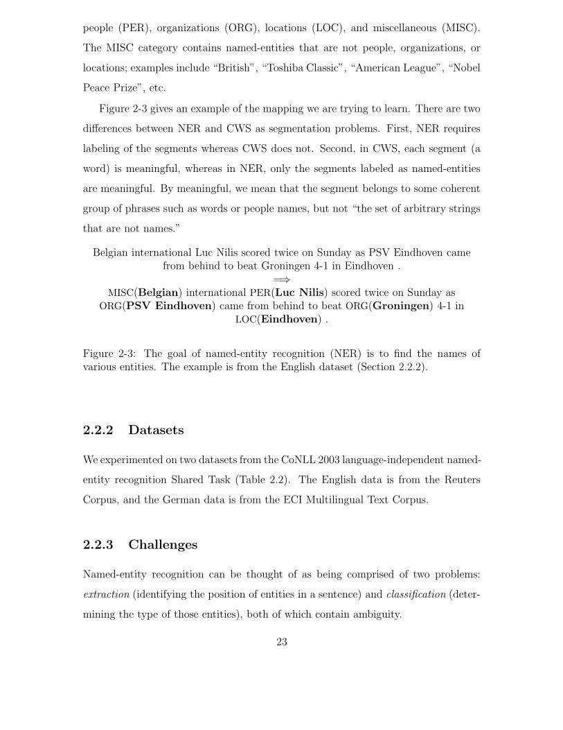
people (PER), organizations (ORG), locations (LOC), and miscellaneous (MISC).
The MISC category contains named-entities that are not people, organizations, or
locations; examples include “British”, “Toshiba Classic”, “American League”, “Nobel
Peace Prize”, etc.
Figure 2-3 gives an example of the mapping we are trying to learn. There are two
differences between NER and CWS as segmentation problems. First, NER requires
labeling of the segments whereas CWS does not. Second, in CWS, each segment (a
word) is meaningful, whereas in NER, only the segments labeled as named-entities
are meaningful. By meaningful, we mean that the segment belongs to some coherent
group of phrases such as words or people names, but not “the set of arbitrary strings
that are not names.”
Belgian international Luc Nilis scored twice on Sunday as PSV Eindhoven camefrom behind to beat Groningen 4-1 in Eindhoven .
=⇒MISC(Belgian) international PER(Luc Nilis) scored twice on Sunday as
ORG(PSV Eindhoven) came from behind to beat ORG(Groningen) 4-1 inLOC(Eindhoven) .
Figure 2-3: The goal of named-entity recognition (NER) is to find the names ofvarious entities. The example is from the English dataset (Section 2.2.2).
2.2.2 Datasets
We experimented on two datasets from the CoNLL 2003 language-independent named-
entity recognition Shared Task (Table 2.2). The English data is from the Reuters
Corpus, and the German data is from the ECI Multilingual Text Corpus.
2.2.3 Challenges
Named-entity recognition can be thought of as being comprised of two problems:
extraction (identifying the position of entities in a sentence) and classification (deter-
mining the type of those entities), both of which contain ambiguity.
23

Sentences Characters Words
Eng. Train 14K 204K 23K
Eng. Dev 3.3K 51K 5.9K
Eng. Test 3.5K 46K 5.6K
Deu. Train 12K 207K 12K
Deu. Dev 2.9K 51K 4.8K
Deu. Test 3K 52K 3.7K
Table 2.2: Statistics of the English (Eng) and German (Deu) named-entity recognitiondatasets from the CoNLL 2003 Shared Task (Sang and Meulder, 2003).
Extraction in English can be driven to some extent by capitalization: capitalized
phrases in the middle of a sentence are likely to be named-entities. However, in
languages such as German, in which all nouns are capitalized, and Chinese, in which
there is no capitalization, one can not rely on this cue at all to find named-entities.
Many models depend on local information to classify named-entities. This can be
troublesome when neither the entity string nor its context provide positive evidence
of the correct entity type. In such cases, the task may be even difficult for a human
who has no prior knowledge about the entity. Consider the sentence “Phillip Morris
announced today that. . . ” The verb “announced” is used frequently following both
people and organizations, so that contextual clue does not help disambiguate the
entity type. “Phillip Morris” actually looks superficially like a person name, and
without a gazetteer of names, it would be difficult to know that “Phillip Morris” is
actually a company.
Sometimes one entity string can represent several entity types, depending on con-
text. For example, “Boston” is typically a location name, but in a sports article,
“Boston” refers to the “Boston Red Sox” organization.
2.2.4 Existing methods
The earliest work in named-entity recognition involved using hand-crafted rules based
on pattern matching (Appelt et al., 1995). For instance, a sequence of capitalized
words ending in “Inc.” is typically the name of an organization, so one could imple-
ment a rule to that effect. However, this approach requires significant hand-tuning
24

to achieve good performance.
Statistical models have proven to be effective with less hand-tuning. Such models
typically treat named-entity recognition as a sequence tagging problem, where each
word is roughly tagged with its entity type if it is part of an entity. Generative models
such as Hidden Markov Models (Bikel et al., 1999; Zhou and Su, 2002) have shown
excellent performance on the Message Understanding Conference (MUC) datasets
(Sundheim, 1995; Chinchor, 1998). These models use a variety of lexical features,
even though the independence assumptions of the generative model are violated.
Discriminative models such as locally-normalized maximum-entropy models (Borth-
wick, 1999) and Conditional Random Fields (McCallum and Li, 2003) have also been
explored for named-entity recognition. (Collins, 2002b) uses a baseline HMM tagger
to generate the best outputs and uses discriminative methods (which take advantage
of a richer set of features) to rerank these outputs. By using semi-Markov Conditional
Random Fields, (Cohen and Sarawagi, 2004; Sarawagi and Cohen, 2004) recast the
named-entity recognition problem as a segmentation problem rather than a tagging
problem. Semi-Markov models also permit a richer set of features. (Miller et al., 2004)
uses a regular Markov model but obtains a richer set of features by using unlabeled
data to derive word clusters.
As mentioned earlier, NER can be viewed as a two-stage problem: (1) find the
named-entities in a sentence, and (2) classify each entity by its type, i.e. person,
organization, location, etc. (Collins, 2002b) mentions that first identifying named-
entities without classifying them alleviates some of the data sparsity issues. (Collins
and Singer, 1999) focuses on the second stage, named-entity classification, assuming
that the named-entities have already been found. They use a bootstrapping approach
based on the co-training framework (Section 3.3.2) to leverage unlabeled examples.
(Riloff and Jones, 1999) uses a similar bootstrapping approach for information ex-
traction.
25

2.3 Evaluation
To evaluate the performance of a method on a segmentation task, we use two standard
measures, precision and recall. Precision is the fraction of segments that the method
produces which are consistent with true segmentation (for named-entity recognition,
the label of the segment must agree with true label as well). Recall is the fraction
of segments in the true segmentation that are consistent with the segmentation the
method produces. Formally:
Precision =|T ∩M |
|M |Recall =
|T ∩M |
|T |
where T is the set of segments in the true segmentation and M is the set of segments
that the method produces. In Chinese word segmentation, T and M include all
segments (words), but in named-entity recognition, T and M only contain segments
corresponding to named-entities.
In general, there is a trade-off between precision and recall. Consider named-
entity recognition. If the method outputs entities very conservatively—that is, it
outputs only if it is absolutely certain of the entity—the method can achieve very
high precision but will probably suffer a loss in recall. On the other hand, if the
method outputs entities more aggressively, then it will obtain a higher recall but lose
precision. A single number that captures both precision and recall is the F1 score,
which is the harmonic mean of precision and recall. One can think of the F1 score as
a smoothed minimum of precision and recall. If both precision and recall are high,
F1 will be high; if both are low, F1 will be low; if precision is high but recall is low,
F1 will be only slightly higher than recall. F1 is formally defined as follows:
F1 =2× Precision × Recall
Precision + Recall
Typically, precision and recall are used in the context of binary classification. For
example, in information retrieval, one task is to classify each document in a set as
relevant or irrelevant and output only the relevant ones. On this task, it is trivial to
26
get 100% recall by outputting all documents, and it is also relatively easy to get very
high precision by outputting the single most relevant document. The segmentation
tasks we consider are different—there is less of this see-saw behavior. For instance, in
named-entity recognition framed as a segmentation problem, a method is not allowed
to output overlapping entities, so it cannot automatically obtain 100% recall. But at
the same time, it can obtain very high precision just as in the information retrieval
case. For Chinese word segmentation, a method cannot output overlapping words as
before, but more interestingly, it cannot trivially achieve high precision either, since
it cannot abstain on sentences it is unsure about. Even if the method finds a word
it is most confident about, it must suggest a segmentation for the characters around
the word and possibly err on those.
27

28

Chapter 3
Learning methods
Section 3.1 sets up the general framework of classification. Section 3.2 covers two
types of global linear models (Markov and semi-Markov models), which provide the
core learning machinery that we use to solve the two segmentation tasks, Chinese
word segmentation and named-entity recognition. Section 3.3 discusses various semi-
supervised learning methods, including our approach of using features derived from
unlabeled data in a supervised model.
3.1 The setup: classification
A wide range of natural language problems, including Chinese word segmentation
(CWS) and named-entity recognition (NER), can be framed as structured classifica-
tion problems. The goal of structured classification is to learn a classifier f mapping
some set X of possible inputs to some set Y of possible outputs using the given train-
ing data. In supervised learning, the input data consists of a set of labeled examples
(x1, y1), . . . , (xm, ym), where each (xi, yi) ∈ X × Y. We are interested in the case of
semi-supervised learning, where in addition to the labeled examples, we receive m′
unlabeled examples xm+1, . . . , xm+m′
.
29

3.2 Global linear models
In this section, we review a general family of models known as global linear models
(GLMs). The key ingredients in a GLM are that (1) the classifier computes a score
for an output which depends linearly on the parameters, and (2) arbitrary global
features can be defined over the entire input and output.
3.2.1 Definition
Formally, a global linear model (Collins, 2004) is specified by the following five com-
ponents:
1. An input domain X and an output domain Y. The domains X and Y define
the problem to be solved. For example, X could be the set of English sentences
(word sequences) and Y, the set of part-of-speech tag sequences; or X could
be the set of Chinese sentences (character sequences) and Y, the set of word
segmentations.
2. A representation feature vector ~Φ : X ×Y → Rd. The domains X and Y might
be symbolic objects, so in order to apply machine learning techniques, we need
to map these objects into real numbers. The (global) feature vector ~Φ(x,y)
summarizes the essential information of (x,y) into a d-dimensional vector. Each
component of ~Φ(x,y) is a (global) feature.
3. A parameter vector ~θ ∈ Rd. The parameter vector ~θ assigns a weight to each
feature in ~Φ(x,y). Together, the value of ~Φ(x,y) ·~θ is the score of (x,y). Higher
scores should indicate that y is a more plausible as an output for x.
4. A function GEN : X → 2Y . GEN(x) is the set of possible outputs y for a given
x. For example, in tagging, GEN(x) is the set of tag sequences of length |x|.
In a reranking problem (Collins, 2000), GEN(x) is a small set of outputs that
have been chosen by some baseline algorithm.
30

5. A decoding algorithm Decode. If we have some parameter vector ~θ, we can use
~θ to classify new examples as follows:
F~θ(x) = arg max
y∈GEN(x)
~Φ(x,y) · ~θ (3.1)
Here, F~θ(x) returns the highest scoring output y out of all candidate outputs
in GEN(x). Decode is an algorithm that either computes F~θ(x) exactly (e.g.,
using exhaustive search or dynamic programming) or approximately (e.g. using
beam search).
If X , Y, ~Φ, ~θ, GEN, and Decode are specified, then we can classify new test
examples. X and Y are defined by the problem; ~Φ, GEN, and Decode are con-
structed so that the representation of the problem is suitable for learning; finally, ~θ
is set through training, which we discuss in Section 3.2.4.
3.2.2 Types of models
So far, we have presented global linear models (GLMs) in an abstract framework. In
this section, we describe two specific types of GLMs for segmentation, Markov and
semi-Markov models, which we use in experiments (Chapter 5).
Markov models
The first type of GLMs that we consider are Markov models (Collins, 2002a; Lafferty
et al., 2001a). In a Markov model, a segmentation can be represented as a sequence
of BIO tags, one tag for each token in the sentence. If segments are not labeled,
as in Chinese word segmentation, then the possible tags are B and I; the first token
(character) of a segment (word) is tagged as B and the rest of the tokens in that
segment are tagged as I. For named-entity recognition, we use B-X and I-X to mark a
segment (entity) with label X; we tag a token (word) as O if that token is not part of
an entity. Note that we cannot collapse B-X and I-X into a single tag or else we would
not be able to differentiate the case when one X entity immediately follows another
31

X entity from the case when there is only one X entity spanning the same words.
Other variants of BIO tagging allocate a new tag for the last word of a segment and
another tag for single-token segments (Xue, 2003).
The output of the named-entity recognition example in Figure 2-3 would be rep-
resented with the following BIO tags (Figure 3-1):
Belgian/B-MISC international/O Luc/B-PER Nilis/I-PER scored/O twice/Oon/O Sunday/O as/O PSV/B-ORG Eindhoven/I-ORG came/O from/O
behind/O to/O beat/O Groningen/B-ORG 4-1/O in/O Eindhoven/B-LOC./O
Figure 3-1: An example of BIO tagging for named-entity recognition.
Formally, a Markov model represents a segmentation y of a sentence x as a se-
quence of tags t1, . . . , t|x|. In a k-th order Markov model, the global feature vector
Φ(x,y) = Φ(x, t1, . . . , t|x|) decomposes into a sum of local feature vectors ~φ(·):
~Φ(x,y) =
|x|∑
i=1
~φ(x, i, ti, ti−1, . . . , ti−k) (3.2)
This decomposition is sufficient for efficient and exact decoding using dynamic
programming (Section 3.2.3). The local feature vector ~φ(x, i, ti, ti−1, . . . , ti−k) ∈ Rd is
associated with the i-th tagging decision and may include any features of the input
sentence x, the current position i, and the subsequence of tags ti . . . ti−k of length k+1.
The current position i is typically used to index the input x at the relevant positions.
Furthermore, we assume that the local feature vector ~φ(·) is actually comprised of d
separate features φ1(·), . . . , φd(·). Then, each component of the d-dimensional global
feature vector can be written as follows:1
Φp(x,y) =
|x|∑
i=1
φp(x, i, ti, ti−1, . . . , ti−k) (3.3)
Typically in NLP, a feature φp is an indicator function. For example, one of the
1Note that we use a subscript, as in φp, to denote a component of a vector and use an arrow or
boldface to denote a full vector, as in ~φ or x.
32
features in our 2nd-order Markov model for NER is the following:
φ3(x, i, ti, ti−1, ti−2) =
1 if xi = Mr. and ti = B-PER and ti−1 = O
0 otherwise.
(3.4)
In this case, Φ3 would just be a count of how many times feature 3 “fired” on the
sentence. In Section 5.1, we specify the full set of features for NER and CWS by
defining a small set of feature templates.
As a technicality, we pad each sentence at the start and at the end with an
unlimited number of special boundary tags and tokens. This allows ~φ to be well-
defined at all positions i from 1 to |x|. At position i = 1, accessing t−2 would simply
return the special boundary token.
By using a k-th order Markov model, a feature cannot depend on two tags that
are farther than distance k apart. In other words, we are making a kth-order Markov
assumption, which is that the tag of a token xi depends only on the tags of a constant-
size neighborhood t[−k...k] around it. Put it another way, ti is conditionally indepen-
dent of all tags in the sequence given the tags in the local neighborhood. This is
a reasonable assumption for part-of-speech tagging, but for segmentation tasks, this
representation may not be adequate.
Semi-Markov models
The second type of GLMs that we consider are semi-Markov models (Sarawagi and
Cohen, 2004). Recall that a feature in a k-th order Markov model can only depend
on a portion of the output corresponding to a length k+1 subsequence of the in-
put sentence (namely, a tag subsequence of length k+1). A feature in a k-th order
semi-Markov model, on the other hand, can be defined on a portion of the output
corresponding to an arbitrarily long subsequence of the input sentence (namely, a sub-
sequence of k+1 arbitrarily long segments). This is arguably a natural representation
for segmentation problems.
More concretely, given a sentence x, a segmentation y consists of m, the number
33

of segments, the starting indices of each segment 1 = s1 < s2 < · · · < sm ≤ |x|, and
the label of each segment l1, . . . lm. The global feature vector decomposes into a sum
of local feature vectors over each local neighborhood of segments, rather than tags:
~Φ(x,y) =
m∑
j=1
~φ(x, sj, sj+1, lj, lj−1, . . . , lj−k) (3.5)
The information available to each feature φp is the entire input sequence x, the
starting and ending positions of the current segment (sj, sj+1−1), and the labels of
the last k+1 segments, including the current segment. For example, in our 1st-order
semi-Markov model for named-entity recognition, we define a local feature as follows:
φ1(x, sj, sj+1, lj, lj−1) =
1 if lj = PER and x[sj :sj+1−1] = “Mr. Smith”
0 otherwise.
(3.6)
Semi-Markov models allow more powerful features to be defined compared to
Markov models. Since segments can be arbitrarily long, a feature in a k-th order
Markov BIO tagging model cannot even consider an entire segment if the segment is
longer than length k. Being able to define features on entire segments can be useful.
For example, in CWS, a useful semi-Markov feature might be an indicator function
of whether the word formed by the characters in the current segment is present in
a dictionary. Such a feature would be more difficult to incorporate into a Markov
model, since words vary in length. An important point is that while features in both
Markov and semi-Markov models can depend on the entire input sequence x, only the
features in a semi-Markov model “knows” where the starting and ending locations
of a segment are, namely (sj, sj+1−1), so that it can use those indices to index the
portion of the input corresponding to the segment.
As in a Markov model, we pad the beginning and end of each sentence with an
unlimited number of length 1 boundary segments, which are labeled with a special
boundary label. Recall that in NER, there are named-entity segments (PER, LOC,
ORG, and MISC) and non-entity segments (O). We set all the non-entity segments
34

to have length 1 in the correct segmentation. For the purposes of decoding, we can
force non-entity segments to also have length 1.
Other models
The simplest example of a GLM is found in the standard linear classification scenario,
where Y contains a constant number of possible outputs. In such a model, a feature
can be defined on the entire input x and output y. The GLM is truly global, but in
a trivial way.
We can also generalize k-th order Markov models beyond sequences to trees (or-
der k = 1) and bounded tree-width graphs (order k > 1), where the dependencies
between tags are not arranged in a linear chain. These general Markov models can
be applicable in parse reranking problems, where a parse tree is fixed, but some sort
of labels are desired at each node. A 1st-order Markov model can be used to define
features on the edges of the tree (Collins and Koo, 2004).
Another natural and more complex class of GLMs are hierarchical models (for
instance, in parsing (Taskar et al., 2004)), where nested labels are assigned over
subsequences of the input. In such a model, a feature may depend on the label of a
subsequence, the labels of the nested subsequences that partition that subsequence,
and the positions of those subsequences.
3.2.3 Decoding
There are two primary reasons for imposing structure in the models we discussed
in Section 3.2.2, instead of allowing arbitrary features over the entire input x and
output y. Requiring the global feature vector to decompose into local features limits
overfitting and allows for tractable exact decoding.
Typically, for structured classification, GEN(x) is exponential in size. For exam-
ple, in tagging, GEN(x) is the set of all tag sequences of length |x|, of which there are
T |x|, where T is the number of tags. It would be too costly to compute F~θ(Equation
3.1) naıvely by enumerating all possible outputs.
35

Fortunately, in Markov and semi-Markov models, we have defined ~Φ(x,y) in a
decomposable way so that decoding can be done exactly in polynomial time. More
generally, case-factor diagrams, which include Markov, semi-Markov, and hierarchical
models, characterize a broad class of models in which ~Φ(x,y) decomposes in a way
that allow this efficient computation (McAllester et al., 2004).
Markov models
The goal of decoding is to compute the maximum scoring tag sequence t1, . . . , t|x|
given an input sequence x. Because the score ~Φ(x,y) · ~θ is linear in ~θ and the global
feature vector ~Φ(x,y) decomposes into a sum over local features that only depend
only on the last k+1 tags, we can solve subproblems of the form “what is the (score of
the) maximum scoring prefix tag subsequence that ends in the k tags ti−k+1, . . . , ti?”
Specifically, we call that value f(i, ti, ti−1, . . . , ti−k+1) and compute it for each length
i using the following recurrence:
f(i, ti, . . . , ti−k+1) = maxti−k
f(i−1, ti−1, . . . , ti−k) + ~φ(x, i, ti, . . . , ti−k) · ~θ (3.7)
The maximum score of a tag sequence is maxti,...,ti−k+1f(|x|, ti, . . . , ti−k+1), and the
optimal tag sequence itself can be recovered by keeping track of the tags ti−k that were
used at each stage to obtain the maximum. This dynamic programming algorithm
(known as Viterbi decoding) runs in O(|x|T k+1) time, where T is the number of tag
types and k is the order of the Markov model.
Semi-Markov models
The dynamic programming for k-th order semi-Markov models has the same flavor as
regular Markov models, with the addition that in the recursion, we need to consider
all possible segment lengths as well as segment labels for the current segment, rather
than just choosing the tag of the current token. Similar to the Markov case, let
f(i, lj, . . . , lj−k+1) be the maximum score of a segmentation ending at position i whose
last k segments are labeled lj−k+1, . . . , lj.
36

Input: Training examples (x1,y1), . . . , (xm,ym), number of iterations TOutput: Parameter vector ~θavg
1~θ ← ~θavg ← 0
2 for t ← 1 to T do3 for i ← 1 to m do
4 y ← Decode(~Φ,xi, ~θ)5 if y 6= yi then
6~θ ← ~θ + ~Φ(xi,yi)− ~Φ(xi,y)
7~θavg ← ~θavg + ~θ
Figure 3-2: The Averaged Perceptron algorithm.
f(i, lj, . . . , lj−k+1) = arg maxlj−k ,n>0
f(i−n, lj−1, . . . , lj−k) + ~φ(x, i−n+1, i, lj, . . . , lj−k) · ~θ
(3.8)The maximum score of a labeled segmentation is maxlj ,...,lj−k+1
f(|x|, lj, . . . , lj−k+1).
This algorithm runs in O(|x|2Lk+1), where L is the number of label types and k is
the order of the semi-Markov model.
3.2.4 Training
Now that we know how to perform decoding using a fixed ~θ to classify new test
examples, how do we train the parameters ~θ in the first place? There are a number
of objectives one can optimize with respect to ~θ and also several types of parameter
estimation algorithms to perform the optimization. In our experiments, we use the
Averaged Perceptron algorithm (Collins, 2002a) mainly due to its elegance, simplicity,
and effectiveness.
Perceptron
The Averaged Perceptron algorithm (Figure 3-2) makes T (typically 20–30) passes
over the training examples (line 2) and tries to predict the output of each training
example in turn (lines 3–4). For each mistake the algorithm makes, the algorithm
nudges the parameters via a simple additive update so as to increase the score of
37

the correct output and decrease the score of the incorrectly proposed output (lines
5–6). The original Perceptron algorithm simply returns the final parameter vector
~θ, but this version suffers from convergence and stability issues. Instead, the Aver-
aged Perceptron algorithm returns the average (or equivalently, the sum) ~θavg of all
intermediate parameters ~θ (which is updated in line 7).
Although the (Averaged) Perceptron algorithm does not seek to explicitly optimize
an objective, the algorithm itself has theoretical guarantees (Freund and Schapire,
1998; Collins, 2002a). If each training example xi is contained in a ball of radius R
and the training set is separable with at least margin δ (∃~θ ∀i,y∈GEN(xi)\yi(~Φ(xi,yi)−
~Φ(xi,y)) · ~θ ≥ δ), then the Perceptron algorithm makes at most R2/δ2 mistakes,
regardless of the input distribution. The Averaged Perceptron algorithm can be seen
as an approximation to the related Voted Perceptron algorithm, which has general-
ization bounds in terms of the total number of mistakes made on the training data
(Freund and Schapire, 1998).
One of the nice properties about the Perceptron algorithm is that it can be used
to train any GLM. The algorithm assumes linearity in ~θ and treats Decode as a
black box. For other parameter estimation algorithms, more complex optimization
techniques or computations other than decoding are required.
3.2.5 Other parameter estimation algorithms
We could use the score ~Φ(x,y) · ~θ to define a conditional probability distribution
P (y|x) = e~Φ(x,y)·~θ
P
y′ e~Φ(x,y′)·~θ
and maximize the conditional likelihood of the training set ex-
amples∏m
i=1 P (yi|xi) (possibly multiplied by a regularization factor). Conditional
Random Fields (CRFs) are Markov models trained according to this criterion (Laf-
ferty et al., 2001a). CRFs have been applied widely in many sequence tasks including
named-entity recognition (McCallum and Li, 2003), Chinese word segmentation (Peng
et al., 2004), shallow parsing (Sha and Pereira, 2003), table extraction (Pinto et al.,
2003), language modeling (Roark et al., 2004), etc. The conditional likelihood can be
efficiently and exactly maximized using gradient-based methods. Finding the gradi-
ent involves computing marginal probabilities P (y|x) for arbitrary y, while at testing
38

time, Viterbi decoding arg maxy P (y|x) is used to find the best y.
Another parameter estimation algorithm is based on maximizing the margin (for
0–1 loss, the margin is δ = mini,y∈GEN(xi)\yi(~Φ(xi,yi) − ~Φ(xi,y)) · ~θ) (Burges, 1998;
Altun et al., 2003; Taskar et al., 2003; Taskar et al., 2004). Like the Perceptron
algorithm, max-margin approaches do not require computing marginal probabilities,
but they do require solving a quadratic program to find the maximum margin. For-
tunately, the constraints of the quadratic program can decompose according to the
structure of the model.
There are a number of variations on basic GLMs. For instance, if there is latent
structure in the input data not represented by the output, we can introduce hidden
variables in order to model that structure (Quattoni et al., 2004). We can also use
kernel methods to allow non-linear classifiers (Collins and Duffy, 2001; Lafferty et al.,
2001b). Instead of working with a fixed feature vector representation ~Φ(x,y), we
can induce the most useful features at training time (Pietra et al., 1997; McCallum,
2003).
3.3 Semi-supervised techniques
3.3.1 Generative maximum-likelihood models
Early research in semi-supervised learning for NLP made use of the EM algorithm
for parsing (Pereira and Schabes, 1992) and part-of-speech tagging (Merialdo, 1994),
but these results showed limited success. One problem with this approach and other
generative models is that it is difficult to incorporate arbitrary, interdependent fea-
tures that may be useful for solving the task at hand. Still, EM has been successful
in some domains such as text classification (Nigam et al., 2000).
3.3.2 Co-training and bootstrapping
A number of semi-supervised approaches are based on the co-training framework
(Blum and Mitchell, 1998), which assumes each example in the input domain can be
39

split into two independent views conditioned on the output class. A natural boot-
strapping algorithm that follows from this framework is as follows: train a classifier
using one view of the labeled examples, use that classifier to label the unlabeled ex-
amples it is most confident about, train a classifier using the other view, use that
classifier to label additional unlabeled examples, and so on, until all the unlabeled
examples have been labeled.
Similar varieties of bootstrapping algorithms have been applied to named-entity
classification (Collins and Singer, 1999; Riloff and Jones, 1999), natural language
parsing (Steedman et al., 2003), and word-sense disambiguation (Yarowsky, 1995).
Instead of assuming two independent views of the data, (Goldman and Zhou, 2000)
uses two independent classifiers and one view of the data.
Both theoretical (Blum and Mitchell, 1998; Dasgupta et al., 2001; Abney, 2002)
and empirical analysis (Nigam and Ghani, 2000; Pierce and Cardie, 2001) have been
done on co-training. (Abney, 2004) analyzes variants of Yarowsky’s bootstrapping
algorithms in terms of optimizing a well-defined objective.
3.3.3 Partitioning
Another class of methods, most natural in the binary case, view classification as par-
titioning examples—both labeled and unlabeled—into two sets. Suppose we define
a similarity measure over pairs of examples and interpret the similarity as a penalty
for classifying the two examples with different labels. Then we can find a minimum
cut (Blum and Chawla, 2001) or a normalized cut (Shi and Malik, 2000) that con-
sistently classifies the labeled examples. Other methods based on similarity between
example pairs include label propagation (Zhu and Ghahramani, 2002), random walks
(Szummer and Jaakkola, 2001), and spectral methods (Joachims, 2003). Transduc-
tive SVMs maximizes the margin of the examples with respect to the separating
hyperplane (Joachims, 1999).
40

3.3.4 Using features derived from unlabeled data
Each of the previous approaches we described attempts to label the unlabeled ex-
amples, either through EM, bootstrapping, or graph partitioning. A fundamentally
different approach, which has been quite successful (Miller et al., 2004) and is the ap-
proach we take, preprocesses the unlabeled data in a step separate from the training
phase to derive features and then uses these features in a supervised model. In our
case, we derive word clustering and mutual information features (Chapter 4) from
unlabeled data and use these features in a Perceptron-trained global linear model
(Section 3.2.4).
(Shi and Sarkar, 2005) takes a similar approach for the problem of extracting
course names from web pages. They first solve the easier problem of identifying
course numbers on web pages and then use features based on course numbers to solve
the original problem of identifying course names. Using EM, they show that adding
those features leads to significant improvements.
41

42

Chapter 4
Extracting features from raw text
In this chapter, we describe two types of features that we derive from raw text:
word clusters (Section 4.1) and mutual information statistics (Section 4.2). We also
describe ways of incorporating these features into a global linear model (Section 4.3).
4.1 Word clustering
One of the aims of word clustering is to fight the problem of data sparsity by providing
a lower-dimensional representation of words. In natural language systems, words
are typically treated categorically—they are simply elements of a set. Given no
additional information besides the words themselves, there is no natural and useful
measure of similarity between words; “cat” is no more similar to “dog” than “run.” In
contrast, things like real vectors and probability distributions have natural measures
of similarity.
How should we define similarity between words? For the purposes of named-
entity recognition, we would like a distributional notion of similarity, meaning that
two words are similar if they appear in similar contexts or that they are exchangeable
to some extent. For example, “president” and “chairman” are similar under this
definition, whereas “cut” and “knife”, while semantically related, are not. Intuitively,
in a good clustering, the words in the same cluster should be similar.
43

4.1.1 The Brown algorithm
In this thesis, we use the bottom-up agglomerative word clustering algorithm of
(Brown et al., 1992) to derive a hierarchical clustering of words. The input to the
algorithm is a text, which is a sequence of words w1, . . . , wn. The output from the
clustering algorithm is a binary tree, in which the leaves of the tree are the words.
We interpret each internal node as a cluster containing the words in that subtree.
Initially, the algorithm starts with each word in its own cluster. As long as there
are at least two clusters left, the algorithm merges the two clusters that maximizes
the quality of the resulting clustering (quality will be defined later).1 Note that the
algorithm generates a hard clustering—each word belongs to exactly one cluster.
To define the quality of a clustering, we view the clustering in the context of a class-
based bigram language model. Given a clustering C that maps each word to a cluster,
the class-based language model assigns a probability to the input text w1, . . . , wn,
where the maximum-likelihood estimate of the model parameters (estimated with
empirical counts) are used. We define the quality of the clustering C to be the
logarithm of this probability (see Figure 4-1 and Equation 4.1) normalized by the
length of the text.
...
...
c1 c2 c3 ci cn
w1 w2 w3 wi wn
P (ci|ci−1)
P (wi|ci)ci = C(wi)
Figure 4-1: The class-based bigram language model, which defines the quality of aclustering, represented as a Bayesian network.
1We use the term clustering to refer to a set of clusters.
44

Quality(C) =1
nlog P (w1, . . . , wn) (4.1)
=1
nlog P (w1, . . . , wn, C(w1), . . . , C(wn)) (4.2)
=1
nlog
n∏
i=1
P (C(wi)|C(wi−1))P (wi|C(wi)) (4.3)
Equation 4.2 follows from the fact that C is a deterministic mapping. Equation 4.3
follows from the definition of the model. As a technicality, we assume that C(w0) is
a special START cluster.
We now rewrite Equation 4.1 in terms of the mutual information between adjacent
clusters. First, let us define some quantities. Let n(w) be the number of times word
w appears in the text and n(w, w′) be the number of times the bigram (w, w′) occurs
in the text. Similarly, we define n(c) =∑
w∈c n(w) to be number of times a word
in cluster c appears in the text, and define n(c, c′) =∑
w∈c,w′∈c′ n(w, w′) analogously.
Also, recall n is simply the length of the text.
Quality(C) =1
n
n∑
i=1
log P (C(wi)|C(wi−1))P (wi|C(wi))
=∑
w,w′
n(w, w′)
nlog P (C(w′)|C(w))P (w′|C(w′))
=∑
w,w′
n(w, w′)
nlog
n(C(w), C(w′))
n(C(w))
n(w′)
n(C(w′))
=∑
w,w′
n(w, w′)
nlog
n(C(w), C(w′))n
n(C(w))n(C(w′))+
∑
w,w′
n(w, w′)
nlog
n(w′)
n
=∑
c,c′
n(c, c′)
nlog
n(c, c′)n
n(c)n(c′)+
∑
w′
n(w′)
nlog
n(w′)
n
We use the counts n(·) to define empirical distributions over words, clusters, and
pairs of clusters, so that P (w) = n(w)n
, P (c) = n(c)n
, and P (c, c′) = n(c,c′)n
. Then the
quality of a clustering can be rewritten as follows:
45

Quality(C) =∑
c,c′
P (c, c′) logP (c, c′)
P (c)P (c′)+
∑
w
P (w) logP (w)
= I(C)−H
The first term I(C) is the mutual information between adjacent clusters and the
second term H is the entropy of the word distribution. Note that the quality of C
can be computed as a sum of mutual information weights between clusters minus the
constant H, which does not depend on C. This decomposition allows us to make
optimizations.
Optimization by precomputation
Suppose we want to cluster k different word types. A naıve algorithm would do the
following: for each of O(k) iterations, and for each of the possible O(k2) possible pairs
of clusters to merge, evaluate the quality of the resulting clustering. This evaluation
involves a sum over O(k2) terms, so the entire algorithm runs in O(k5) time.
Since we want to be able to cluster hundreds of thousands of words, the naıve
algorithm is not practical. Fortunately, (Brown et al., 1992) presents an optimization
that reduces the time from O(k5) to O(k3). The optimized algorithm maintains
a table containing the change in clustering quality due to each of the O(k2) merges
(Brown et al., 1992). With the table, picking the best merge takes O(k2) time instead
of O(k4) time. We will show that the table can be updated after a merge in O(k2)
time.
Instead of presenting the optimized algorithm algebraically (Brown et al., 1992),
we present the algorithm graphically, which we hope provides more intuition. Let a
clustering be represented by an undirected graph with k nodes, where the nodes are
the clusters and an edge connects any two nodes (clusters) that are ever adjacent to
each other in either order in the text. Note there might be self-loops in the graph.
Let the weight of an edge be defined as in Equation 4.4 (see below). One can verify
that the total graph weight (the sum over all edge weights) is exactly the mutual
46

information I(C) = Quality(C) + H, which is the value we want to maximize.
w(c, c′) =
P (c c′) log P (c c′)P (c)P (c′)
+ P (c′ c) log P (c′ c)P (c′)P (c)
if c 6= c′
P (c c) log P (c c)P (c)P (c)
if c = c′.
(4.4)
Note that we can keep track of P (c), P (c, c′), w(c, c′) without much difficulty. The
table central to the optimization is L(c, c′). For each pair of nodes (c, c′), L(c, c′) stores
the change in total graph weight if c and c′ were merged into a new node. (Our L(c, c′)
has the opposite sign of L in (Brown et al., 1992)). Figure 4-2(a) and Equation 4.5
detail the computation of L(c, c′). We denote the new node as c∪c′, the current set of
nodes as C, and the set of nodes after merging c and c′ as C ′ = C −{c, c′}+ {c∪ c′}.
L(c, c′) =∑
d∈C′
w(c ∪ c′, d)−∑
d∈C
(w(c, d) + w(c′, d)) (4.5)
For each node c, (Brown et al., 1992) also maintains s(c) =∑
c′ w(c, c′), the sum
of the weights of all edges incident on c. We omit this, as we can achieve the same
O(k3) running time without it.
At the beginning of the algorithm, L(c, c′) is computed in O(k) for each pair of
nodes (c, c′), where k is the number of nodes (Equation 4.5, Figure 4-2(a)). Summing
over all pairs, the total time of this initialization step is O(k3).
After initialization, we iteratively merge clusters, choosing the pair of clusters to
merge with the highest L(c, c′). This takes O(k2) time total (for each pair (c, c′), it
takes O(1) time to look up the value of L(c, c′)). After each merge, we update L(c, c′)
for all the pairs (c, c′) in O(k2) total time as follows: For each (c, c′) where both c and
c′ were not merged, ∆L(c, c′) is computed in O(1) time by adding and subtracting
the appropriate edges in Figure 4-2(b). For the remaining pairs (c, c′) (of which
there are O(k)), we can afford to compute L(c, c′) from scratch using Equation 4.5
(Figure 4-2(a)), which takes O(k) time. Thus, all the updates after each merge can
be performed in O(k2) time total. As O(k) total merges are performed, the total
running time of the algorithm is O(k3).
47
c’c
L(c, c′) (O(k) time)
......
(a) Computed from scratch
O(k) nodes︷ ︸︸ ︷
∆L(c, c′) (O(1) time)
c’c
(b) Computed after each merge
the new merged node
added edge (weight to be added)
deleted edge (weight to be subtracted)
number of nodes = O(k)
number of edges = O(k2)
Figure 4-2: Visualizing the Brown algorithm. (a) shows the edges involved in com-puting L(c, c′) from scratch (solid indicates added, dashed indicates subtracted). (b)shows the edges involved in computing ∆L(c, c′), the change in L(c, c′) when the twonodes in the shaded box have just been merged.
Optimization using a fixed window size
Even an O(k3) algorithm is impractical for hundreds of thousands of words, so we
make one further optimization. But unlike the previous optimization, the new one
does not preserve functionality.
We fix a window size w and put each of the w most frequent words in its own
cluster. L(c, c′) is then precomputed for each pair of clusters (c, c′). This initialization
step takes O(w3) time.
Then, for each of the remaining k−w words that have not been placed in a cluster,
we add the word to a new cluster cw+1. We then need to update two things: (1) the
edge weights and (2) the L(c, c′) entries involving cw+1.
Assume that, as we were initially reading in the text, we computed a hash table
mapping each word to a list of neighboring words that appear adjacent to it in the
text. To compute the edge weights between the new cluster cw+1 and the first w
clusters, we loop through the words adjacent to the new word in cw+1, keeping track
of the counts of the adjacent words’ corresponding clusters. The edge weights can be
easily calculated given these counts. The total time required for this operation over
the course of the entire algorithm is O(T ), where T is the length of the text.
After the edge weights are computed, L(c, c′) can be updated easily. O(1) time
is required for each cluster pair that does not include cw+1; O(w) time is otherwise
48

required to do the computation from scratch (Figure 4-2(a)). Thus, the total time
spent in creating new clusters is O(kw2 + T ).
Now we merge the optimal pair of clusters among the resulting w+1 clusters in
the same way as in the first optimized algorithm. That algorithm took O(k2) time
for each merge because there were k clusters, but since there are only w clusters at a
time in the new algorithm, the time required is O(kw2) total to introduce the k − w
words to the current clustering.
This new algorithm runs in O(kw2 + T ), where k is the number of words we want
to cluster and w is the initial window size of frequent words. In practice, k = 250, 000
and w = 1000. The algorithm is still slow but practical.
Word similarity
Revisiting our motivating notion of word similarity, note that we do not formally
define the similarity between two words, even though we would like our algorithm to
place similar words in the same cluster. Fortunately, the quality of a clustering turns
out to encourage words with similar contexts to be merged into the same cluster.
As a simple example, consider two words wa and wb which have similar contexts.
In fact, assume their left and right adjacent word distributions are identical. For
simplicity, also assume that they never occur next to each other. We will show that
the clustering quality stays the same if we merge wa and wb into one cluster. Let w
be any other word. The clustering quality prior to merging wa and wb includes the
two terms A = P (w, wa) log P (w,wa)P (w)P (wa)
and B = P (w, wb) log P (w,wb)P (w)P (wb)
, which sums to
(P (w, wa)+ P (w, wb)) log P (w,wa)P (w)P (wa)
, since P (w,wa)P (wa)
= P (w,wb)P (wb)
. After merging wa and wb
into cluster cab, the A + B is replaced by P (w, cab) log P (w,cab)P (w)P (wab)
which is identical to
A + B since P (w, cab) = P (w, wa) + P (w, wb). Since the clustering quality is always
monotonically non-increasing with successive merges, the algorithm will always merge
two words with the identical contexts if it can.
49

Variants of the Brown algorithm
(Martin et al., 1995) extends the Brown algorithm by using an objective function
based on trigram models instead of bigram models. They also introduce an efficient
exchange algorithm that tries to improve the objective by moving words from one
cluster to another. The exchange technique was also used in (Ushioda, 1996).
Relation to HMM learning
Figure 4-1 bears a striking resemblance to a Hidden Markov Model (HMM), and we
can view the problem of finding a good clustering C as the problem of learning an
HMM. However, note that each observation (token) in an HMM produced by the
Brown algorithm is emitted by exactly one state (cluster). This is not true for HMMs
in general.
The method of merging clusters or states in an HMM like the Brown algorithm has
also been explored by (Stolcke and Omohundro, 1993) in Bayesian model merging.
In that work, they start with each occurrence of a word in a different state, whereas
the Brown algorithm starts with each word type in a different state. At any point in
time, the Brown algorithm always assigns a hard clustering to words, but (Stolcke
and Omohundro, 1993) allows the possibility of a soft clustering, which happens when
the initial states of two word occurrences are not merged together. Also, (Stolcke and
Omohundro, 1993) places a Dirichlet prior on the model (the clustering) and decides
on the best merge with respect to maximizing the posterior P (C|w) ∝ P (w|C)P (C)
rather than with respect to the likelihood P (w|C). The prior provides a natural stop-
ping point—when the posterior cannot be increased by merging two clusters. Note
that the likelihood P (w|C) never increases, so it cannot provide a natural stopping
point. However, committing to a particular stopping point is not necessary, since
we can use the full hierarchical clustering produced by the Brown algorithm in a
discriminative model.
An HMM can also be learned using the Baum-Welch algorithm. However, Bayesian
model merging yields better models compared to the models produced by the Baum-
50

1: February December March October November April September January May August ...2: Benjamin Rudolph Sammy Al Henry Mark George Paul ...
3: accusations regulations lawsuits threats allegations sanctions measures legislation laws ...4: Afghanistan Spain Canada Europe Asia Italy Ireland Germany Mexico France ...
...
Figure 4-3: Examples of English word clusters.
Welch algorithm (Stolcke and Omohundro, 1993). Another way to produce more
meaningful models is to place an entropic prior on the parameters of the HMM, so
that there is a bias towards models with more deterministic transition probabilities
(Brand, 1999).
4.1.2 Extracting word clusters
Using the Brown algorithm, we produced two sets of word clusters, one for English
and one for German. To prepare the English clusters, we used the 1996 Reuters text
from the LDC, which is the source of the CoNLL 2003 English named-entity data.
We stripped out any paragraphs that do not resemble real sentences, i.e., ones that
are composed of less than 90% lowercase letters a–z. We ran the algorithm on the
cleaned text (43M words, 280K word types), starting with 1000 initial clusters. The
clustering took 77 hours on a 2.8 GHz processor. Some examples of word clusters are
shown in Figure 4-3.
To prepare the German clusters, we used the 2003 European Parliamentary pro-
ceedings (27M words, 283K word types). We did not have access to the ECI Multilin-
gual Text Corpus, which was the source of the German named-entity data. Starting
with 1000 clusters, the clustering algorithm took 74 hours.
4.1.3 Utility of word clusters
As mentioned earlier, word clustering alleviates the data sparsity problem by allowing
the learning algorithm to draw analogies between different words. In named-entity
recognition, for example, we might leverage cues such as the nearby occurrence of
the word “chairman” to signify a person entity. But “chairman” is not unique in this
51

role. In fact, words that are similar to “chairman”—such as “author” or “founder” or
“CEO”—could also play the part. Without word clustering, the learning algorithm
cannot make a connection between these words. With word clustering information,
the learning algorithm can learn, not just that the word “chairman” is indicative of
a person entity, but that the entire cluster containing “chairman” is indicative of a
person entity.
We now support the intuition with a simple experiment. We collected all the
single-word names of people in the English NER training set (2316 occurrences, 968
types). Each person name belongs to one of the 1000 leaf word clusters, and this
induces a distribution of leaf word clusters over all single-word person names. The
entropy of this distribution is 2.92 bits. For the control experiment, we collected 2316
words drawn randomly from the training set text. The entropy of that distribution
was 8.13 bits. Clearly, the word clusters have managed to capture some distributional
property that binds together people names. Instead, consider all the words that
precede a person name (6600 occurrences, 796 types). The entropy of the induced
distribution is 5.69 bits, whereas the random baseline is 8.37 bits. Here, the signal
provided by the word clusters is much weaker, which is not surprising given that
people names can be used in a variety of contexts.
4.2 Mutual information
The second type of feature that we extract from raw text is (pointwise) mutual
information (MI). MI is a standard measure of the strength of association between
co-occurring items and has been used successfully in extracting collocations from
English text (Lin, 1998) and performing Chinese word segmentation (Sproat and
Shih, 1990; Maosong et al., 1998; Zhang et al., 2000; Peng and Schuurmans, 2001b).
Fortunately, it is simple to derive estimates of mutual information from unlabeled
data (raw unsegmented text) alone. Unlike word clustering, MI can be computed
quickly—in time linear in the text length. The MI of two Chinese characters x1 and
x2 is computed as follows:
52

MI(x1, x2) = logP (x1 x2)
P (x1 )P ( x2)(4.6)
Here P (x1 x2) is an estimate of the probability of seeing x1 followed by x2; P (x1 )
and P ( x2) are marginal probabilities.
4.2.1 Extracting mutual information
To estimate MI values, we used the text from the four Bakeoff datasets, combined
with an amalgamation of the Chinese part of nine different parallel corpora from
the LDC. This parallel corpora includes FBIS, Hong Kong Hansards, UN Corpus,
Xinhua News Corpus, etc. The entire raw text we use contains 90M characters, 10K
character types, and 1.9M character bigram types. We used add-one smoothing on
all the unigram and bigram counts. Table 4.1 presents some examples of MI values.
We find that two characters with high MI tend to belong to the same word, and
two characters with low MI tend to belong to different words. The next section will
attempt to demonstrate this correlation.
Character pair Mutual information Is a word?���shan xı (a province in China) 6.78 yes���
shan guang (flash) 5.53 yes���yue san (month 3) 3.21 no�an wen (steady) 1.59 yes�� da gou (big dog) 0.00 no
��� yı duı (a couple) -1.44 yes���wo bıng (I sick) -3.52 no���
he xie (and some) -5.11 no� �guo yue (country month) -5.41 no
Table 4.1: Mutual information values of various Chinese character pairs.
4.2.2 Utility of mutual information
MI would be helpful for CWS if word boundaries are more likely to occur between
two characters with low MI than with high MI. To see if there is a correlation, we
53

Average mutual information Number of character pairsSpans a boundary 0.691 637,008Within a word 3.982 991,141
Table 4.2: Mutual information across word boundaries is much lower than mutualinformation within words. The test was done on the PK Train set.
compared the MI of adjacent characters that span a word boundary with the MI of
adjacent characters within a word (Table 4.2).
From this simple experiment, we conclude that there is a correlation between
word boundaries and mutual information. Consider a simple heuristic based purely
on mutual information: to decide whether two adjacent characters should be part of
the same word, compare the MI between the two characters against a fixed threshold
t; place a word boundary if and only if the MI is smaller than t. If we choose t simply
to be the halfway point between the two average mutual information values 0.691
and 3.982 (t = 2.34), we can detect word boundaries with 84.9% accuracy. If we had
known the optimal threshold t = 2.4 a priori, we could have obtained 85% accuracy.
4.3 Incorporating features from unlabeled data
In this section, we discuss how we incorporate the information derived from unlabeled
data into a global linear model and give examples for a Markov model. The full set
of features is given in Section 5.1.
4.3.1 Using word cluster features
Recall that each component of the global feature vector of a GLM decomposes into
a sum of local features. To use our word clusters, we add indicator features that
fire when a word is in a given cluster. For example, suppose a cluster C25 contains
the words “Mark”, “Al”, “Paul”, etc. Based on the discussion in Section 4.1.3, we
would expect the feature in Equation 4.7 to be useful in the Markov model. The
feature returns 1 if and only if a word belonging to a cluster containing mostly first
names is tagged as the beginning of a person name. Of course we have no way of
54

knowing the usefulness of such a feature a priori, so we add all features of this same
form, where C25 and B-PER are replaced by any other cluster and tag, respectively
(Section 5.1). We have simply highlighted one feature that might be useful and thus
would be assigned a positive weight during training.
φ38(x, i, ti, ti−1, ti−2) =
1 if xi ∈ C25 and ti = B-PER
0 otherwise.
(4.7)
Since the Brown algorithm produces hierarchical clusters, from which level in the
hierarchy should we pick clusters to use in our features? We do not know in advance
what clustering granularity would be appropriate for NER. Fortunately, GLMs al-
low arbitrary overlapping features, so we can add clustering features corresponding
to multiple levels of the hierarchy. The hope is that the learning algorithm will au-
tomatically choose the ones that are most useful for the task and assign them high
weight. Following (Miller et al., 2004), we use a cluster (a node in the tree) in features
if it has a depth (distance from the root node) that is a multiple of 4 or it is a leaf of
the tree.
4.3.2 Using mutual information features
Mutual information (MI) values are trickier to incorporate than word clusters because
they are continuous rather than discrete. As an example of how MI statistics might
be incorporated into a GLM, we could define a local feature that either returns the
MI value or 0:
φ7(x, i, ti, ti−1, ti−2) =
MI(xi−1, xi) if ti−1 = B and ti = I
0 otherwise
(4.8)
The mutual information values that we obtained in Section 4.2.1 span the range
from -9.88 to 17.6 (Figure 4-4). Since all other feature values we have discussed take
on binary values of 0 or 1, there is a “mis-match” between the continuous and binary
features. As we show later, GLMs can be sensitive to inappropriately scaled feature
55

values.
0
500
1000
1500
2000
2500
3000
-5 0 5 10 15
Figure 4-4: A histogram showing the distribution of mutual information values esti-mated from unsegmented Chinese text.
We consider three ways of dealing with this mis-match by transforming the MI
values into a more amenable form to use in the GLM:
• Scale and translate the MI values so that they are contained in some fixed range
[a, b]. The smallest MI value maps to a, and the largest MI value maps to b.
• Replace the MI values with their z-scores. The z-score of a MI value x is x−µ
σ,
where µ and σ are the mean and standard deviation of the MI distribution,
respectively.
• Convert the continuous MI values into binary values by thresholding at some
δ. In other words, map a raw MI value x to a if x < δ and b if x ≥ δ. In our
experiments, we set δ to µ, the mean MI value.
We experiment with these three approaches on the HK dataset. The features and
experimental setup we used are described in Chapter 5: we trained a Markov model
using the Perceptron algorithm on 10% of the available training data for 20 iterations.
Table 4.3 gives the performance on the Dev set.
56

Method F1 score on Dev
Without MI values 77.08
Raw MI values 81.51
Threshold at mean to {0, 1} 80.83
Threshold at mean to {-1, 1} 80.47
Normalize to [-3, 3] 82.90
Normalize to [-1, 1] 83.19
Normalize to [0, 1] 83.27
Z-score 83.35
Multiply by 10 68.89
Table 4.3: F1 scores obtained by using various ways to transform mutual informationvalues before using them in a Markov model. The experiments were done on the HKdataset. 10% of the total available training data (29K characters) was used.
Although using raw MI values directly in features (Equation 4.8) does improve
performance over the baseline (from 77.08% to 81.51%), it is helpful to rescale the
MI values to make them more friendly for the GLM. Thresholding actually performs
worse than using raw MI values, since we are probably losing too much information.
By normalizing the MI values in various ways, we can increase the performance as
compared to using raw MI values. We obtain the highest performance by normalizing
with z-scores (81.35%). Finally, to demonstrate the brittleness of the model due to
arbitrary feature scaling, we purposely multiplied the raw MI values by 10 to make
the features span even a larger range. As a result, performance plummets to 68.89%.
57

58

Chapter 5
Experiments
In this section, we present experiments on a total of five datasets (Eng, Deu, CTB,
PK, and HK). Eng and Deu are named-entity recognition datasets from the CoNLL
2003 Shared Task (Section 2.2.2). CTB, PK, and HK are from the 2003 Chinese
Word Segmentation Bakeoff (Section 2.1.3). For each dataset, we measure (1) the
effect of using a semi-Markov versus a Markov model and (2) the effect of adding
features derived from unlabeled data. We are also interested in these effects when we
are training with a small amount of labeled data. We trained the various models on
5%, 10%, 20%, 50%, and 100% of the available sentences. Section 5.1 describes the
features we used in the different models, and Section 5.2 presents the results of our
experiments.
5.1 Features
Recall that in a 2nd-order Markov model, the global feature vector is a sum of local
feature vectors ~φ(x, i, ti, ti−1, ti−2), where x is the input sentence, i is the current
position, and ti, ti−1, ti−2 are the last three tags (Equation 3.2). In NLP applications,
a local feature vector typically contains millions of components (features), which are
described compactly using feature templates. Each feature template represents a set
of features. For example, the feature template denoted as (ti, xi+1) describes the set
59
of features of the form:
φp(x, i, ti, ti−1, ti−2) =
1 if ti = ? and xi+1 = ?
0 otherwise,
where the question marks can be filled in with any strings. In practice, only
the strings encountered during the training process actually matter; if a string is
never encountered, the corresponding feature will always have weight 0. In the above
example, the first question mark can be replaced by any of the possible tags (B-PER,
I-PER, B-ORG, I-ORG, B-LOC, I-LOC, B-MISC, I-MISC, and O), and the second
question mark can be replaced by any word that appears in the training set. Note
that if a word is observed in the test set but not in the training set, then that word
would only trigger features that have weight 0.
Figures 5-1 to 5-4 list the feature templates used in the Markov and semi-Markov
models for CWS and NER. We opted for simple and clean features. The NER training
sets were also annotated with part-of-speech and noun phrase chunking information,
which we did not use. Preliminary experimentation showed that the additional in-
formation does not provide a substantial improvement when we are already using
unlabeled data features. Each word in the German training set was also annotated
with its lemmatized form, which we ignored as well.
Each line in Figures 5-1 to 5-4 describes multiple feature templates. For example,
consider line 5 in Figure 5-1 ((ti, xi+∆) for ∆ ∈ {−2,−1, 0, 1, 2}). The five feature
templates described by this line are (ti, xi−2), (ti, xi−1), (ti, xi), (ti, xi+1), and (ti, xi+2);
each feature template in turn defines a set of features. In general, xi+∆ refers to the
token at position i + ∆, where i is the current position; ti+∆ refers to the tag at
position i + ∆.
For a 1st-order semi-Markov model, each local feature is defined as φp(x, sj, sj+1, lj, lj−1).
In Figures 5-2 and 5-4, s = sj and e = sj+1−1 are the starting and ending positions of
the current segment, and (li, li−1) are the labels of the current and previous segments.
60

For example, line 7 in Figure 5-2 (lj, xs...e) includes features of the following form:
φp(x, sj, sj+1, lj, lj−1) =
1 if lj = ? and x[sj :sj+1−1] = ?
0 otherwise,
In addition to the basic indicator feature templates on tags and tokens, the CWS
feature templates (Figures 5-1 and 5-2) based on unlabeled data features involve re-
turning the mutual information z-score of two characters MIz(xi, xi+1) (Section 4.3.2).
Some of the NER feature templates (Figures 5-3 and 5-4) involve two sets of string
operations, C and M, where a string is simply a word or a subsequence of words.
Each operation maps strings to equivalence classes. If these equivalence classes are
relevant to NER, then this lower-dimensional representation of strings can be useful
for generalization. Features can be defined in terms of equivalence classes rather than
the actual strings.
• M is a set of 11 orthographic transformations that map a string to another
string via a simple surface level transformation. The functions m(x) ∈ M
include the following:
1 Map x to its uncapitalized form (e.g., “Smith” → “smith”)
2 Return the type of x, obtained by replacing [a-z] with a, [A-Z] with A, and
[0-9] with 0 (e.g., “D. E. Shaw” → “A. A. Aaaa”)
3 Return the type of x, except successive repeated characters are replaced with
a single occurrence (e.g., “D. E. Shaw” → “A. A. Aa”)
4–7 Return the first n characters of x, where 1 ≤ n ≤ 4 (e.g., “reporter” →
“re” if n = 2)
8–11 Return the last n characters of x, where 1 ≤ n ≤ 4 (e.g., “reporter” →
“ter” if n = 3)
• Each operation in C maps a word to a cluster identity (Section 4.3.1). One
operation c(x) ∈ C maps the word x to the leaf cluster containing x. The
61

other operations c(x) ∈ C map the word x to the clusters at depths 4, 8, 12, . . .
containing x. If x was not seen while constructing the clusters and thus does
not belong to any cluster, then it is mapped to a special NULL cluster.
In each of the 4 figures (Figures 5-1 to 5-4), the feature templates are divided into
regular and unlabeled data feature templates. The baseline Markov and semi-Markov
models, which we denote M and SM, respectively, use only the regular features.
Markov and semi-Markov models that use both regular and unlabeled data features
are denoted M+F and SM+F, respectively. Section 5.2 describes experiments using
all four models.
CWS: Markov
Regular features:
1 ti2 ti, ti−1
3 ti, ti−1, ti−2
4 ti, ti−1, xi, xi−1
5 ti, xi+∆ for ∆ ∈ {−2,−1, 0, 1, 2}6 ti, xi+∆, xi+∆+1 for ∆ ∈ {−2,−1, 0, 1}
Features based on mutual information:
7 ti,MIz(xi−1, xi)
Figure 5-1: Markov model features for CWS. ti is the current tag, xi is the currentcharacter, and MIz(xi−1, xi) is the mutual information z-score of the previous andcurrent characters.
CWS: semi-Markov
Regular features:
1 lj2 lj , lj−1
3 lj , xi for i ∈ {s−2, s−1, s, e, e+1, e+2}4 lj , xi, xi+1 for i ∈ {s−2, s−1, e, e+1}5 lj , xs...e
Features based on mutual information:
6 lj , lj−1,MIz(xs−1, xs)7 lj ,MIz(xs...e)
Figure 5-2: Semi-Markov model features for CWS. lj is the current segment label; sand e are the starting and ending indices of the current segment, respectively.
62

NER: Markov
Regular features:
1 ti2 ti, ti−1
3 ti, ti−1, ti−2
4 ti, ti−1, xi, xi−1
5 ti,m(xi+∆) for ∆ ∈ {−1, 0, 1},m ∈M6 ti, xi+∆, xi+∆+1 for ∆ ∈ {−1, 0}
Features based on word clusters:
7 ti, c(xi+∆) for ∆ ∈ {−1, 0, 1}, c ∈ C8 ti, c(xi+∆), c(xi+∆+1) for ∆ ∈ {−1, 0}, c ∈ C9 ti, ti−1, c(xi), c(xi−1) for c ∈ C
Figure 5-3: Markov model features for NER. C andM are sets of string operations.
NER: semi-Markov
Regular features:
1 lj2 lj , lj−1
3 lj ,m(xi) for i ∈ {s−1, s, e, e+1},m ∈M4 lj , xi+∆, xi+∆+1 for ∆ ∈ {s−1, e}5 lj ,m(xs...e) for m ∈M′
Features based on word clusters:
6 lj , c(xi) for i ∈ {s−1, s, e, e+1}, c ∈ C7 lj , c(xi), c(xi+1) for i ∈ {s−1, e}, c ∈ C8 lj , c(xs...e) for c ∈ C
Figure 5-4: Semi-Markov model features for NER.
Limiting the segment length A standard semi-Markov model as defined in Sec-
tion 3.2.2 does not bound the allowable length of a segment. But for NER and CWS,
it is not necessary to consider segments that are arbitrarily long. Pruning long seg-
ments increases the efficiency of the algorithm without noticeably affecting accuracy.
We modify the decoding algorithm in Section 3.2.3 to only consider segments of up to
length P . We choose P as small as possible while ensuring that 99.9% of the segments
in the Train set are no longer than P tokens. The first number in the Train column
of Table 5.1 shows values of P for the different datasets. These values of P are used
in both training and testing on Train, Dev, and Test.
Making this restriction improves the running time of the Viterbi decoding algo-
rithm (Section 3.2.3) from O(|x|2L2) to O(|x|PL2), where |x| is the length of the
63

Train Dev Test
CTB 8 (max 21) 8 (max 10) 5 (max 9)PK 6 (max 22) 6 (max 13) 5 (max 13)HK 7 (max 14) 6 (max 9) 6 (max 14)Eng 6 (max 10) 7 (max 10) 5 (max 6)Deu 7 (max 18) 6 (max 8) 7 (max 9)
Table 5.1: For each dataset (CTB, PK, etc.) and each of its three sets of examples(Train, Dev, and Test), we show the bound on the segment length as computed fromthe examples in that set, as well as the maximum segment length. Note that onlythe bounds computed from the Train set are used in training and testing.
input and L is the number of label types. Recall that the running time for decoding
a 2nd-order Markov model is O(|x|T 3), where T is the number of tags. For NER,
the number of labels L is 5. Since there is a B-X and a I-X tag for each label X
except O, the number of tags T is 9. From Table 5.1, we can see that P is not only
much smaller than |x| but also less than T . It seems quite possible that training and
decoding 1st-order semi-Markov models would be faster than training and decoding
2nd-order Markov models. Indeed, our experiments show this to be the case: for
NER, the time required to train semi-Markov models is only a third of the time re-
quired for Markov models. For CWS, the time is around 30% less for semi-Markov
models.
5.2 Results
We conducted experiments on the five datasets: CTB, PK, HK, Eng, and Deu. On
each dataset, we tried 4 different methods—a Markov model (M), a Markov model
with unlabeled data features (M+F), a semi-Markov model (SM), and a semi-Markov
model with unlabeled data features (SM+F). For each dataset and method, we trained
a model using various fractions of the total available training data: 5%, 10%, 20%,
50%, and 100%. We chose the sentences randomly and average over 5 trials. In
each experiment, we trained the model using the Averaged Perceptron algorithm
(Section 3.2.4) for 20 iterations.
Tables 5.2 to 5.6 show the precision, recall, and F1 scores on the Test set for each
64

of the 4 different methods for each of the 5 datasets. Each number is accompanied
with the standard deviation over the 5 trials. The numbers obtained from using 10%
and 100% of the total training data are reported. Figures 5-5 to 5-9 plot the F1 scores
of the 4 methods as the amount of labeled training data increases.
Method, train. frac. Precision Recall Test F1
M 10% 78.2 ±0.29 75.0 ±0.74 76.6 ±0.51
M 100% 86.0 83.9 84.9M+F 10% 81.7 ±0.09 81.7 ±0.48 81.7 ±0.26
M+F 100% 88.0 87.8 87.9SM 10% 78.1 ±0.44 75.3 ±0.43 76.7 ±0.39
SM 100% 85.8 83.6 84.7SM+F 10% 81.1 ±0.25 81.8 ±0.21 81.4 ±0.20
SM+F 100% 86.9 86.6 86.8
Table 5.2: Results on the CTB (Test) dataset.
Method, train. frac. Precision Recall Test F1
M 10% 87.3 ±0.18 86.0 ±0.15 86.6 ±0.15
M 100% 93.4 92.5 92.9M+F 10% 89.9 ±0.13 89.6 ±0.20 89.7 ±0.15
M+F 100% 94.1 94.1 94.1SM 10% 87.8 ±0.24 87.4 ±0.21 87.6 ±0.20
SM 100% 93.5 93.2 93.3SM+F 10% 89.9 ±0.17 88.8 ±0.22 89.4 ±0.18
SM+F 100% 94.0 93.2 93.6
Table 5.3: Results on the PK (Test) dataset.
Method, train. frac. Precision Recall Test F1
M 10% 83.0 ±0.43 82.0 ±0.41 82.5 ±0.38
M 100% 92.3 91.9 92.1M+F 10% 86.9 ±0.30 87.2 ±0.31 87.0 ±0.25
M+F 100% 93.6 93.9 93.7SM 10% 84.0 ±0.22 82.3 ±0.38 83.1 ±0.23
SM 100% 93.1 92.0 92.5SM+F 10% 87.3 ±0.22 87.3 ±0.49 87.3 ±0.29
SM+F 100% 93.6 93.5 93.6
Table 5.4: Results on the HK (Test) dataset.
Tables 5.7 and 5.8 compare our results with related methods based on Conditional
Random Fields for CWS (Peng et al., 2004; Li and McCallum, 2005) and NER
(McCallum and Li, 2003). The CRF of (Li and McCallum, 2005) uses word clustering
features derived from an HMM-LDA model, which is similar to our approach. The two
65

Method, train. frac. Precision Recall Test F1
M 10% 72.9 ±0.49 71.3 ±0.63 72.1 ±0.54
M 100% 82.7 82.1 82.4M+F 10% 80.0 ±0.64 78.7 ±0.72 79.4 ±0.44
M+F 100% 87.6 87.1 87.3SM 10% 74.1 ±0.40 72.4 ±0.60 73.2 ±0.15
SM 100% 82.4 81.2 81.8SM+F 10% 81.9 ±0.82 80.3 ±0.90 81.1 ±0.72
SM+F 100% 87.4 86.8 87.1
Table 5.5: Results on the Eng (Test) dataset.
Method, train. frac. Precision Recall Test F1
M 10% 66.6 ±2.05 40.5 ±0.87 50.4 ±0.79
M 100% 79.1 58.0 66.9M+F 10% 65.8 ±1.72 45.4 ±0.62 53.7 ±0.77
M+F 100% 78.8 62.6 69.8SM 10% 64.5 ±1.08 42.0 ±0.40 50.9 ±0.57
SM 100% 78.4 60.2 68.1SM+F 10% 65.4 ±0.78 47.4 ±0.73 55.0 ±0.57
SM+F 100% 77.6 62.6 69.3
Table 5.6: Results on the Deu (Test) dataset.
CRFs for CWS of (Peng et al., 2004) are trained using an open and a closed feature
set. The open set includes external information such as lexicons from the Internet,
while the closed set only contains the lexicon induced from the training data. While
our M+F and SM+F models technically do use external information, this information
is in the form of raw text and does not require human effort to process. On CWS,
M+F surpasses CRF with the closed feature set and approaches CRF with the open
feature set. Note that our models are trained on the Train set we created, which
excludes the Dev set, whereas the CRF models are trained on both Train and Dev.
On NER, both M+F and SM+F outperform CRF, which uses external information
such as gazetteers collected automatically from the Internet.
5.2.1 Effect of using unlabeled data features
Having painted an overall picture of our results, we now examine the specific contribu-
tions of adding unlabeled data features (M→ M+F and SM→ SM+F). Tables 1 to 4
in the Appendix show that the error is reduced significantly on all datasets, in some
cases by as much as 30%. The reduction is the greatest when smaller amounts of the
66

0.7
0.72
0.74
0.76
0.78
0.8
0.82
0.84
0.86
0.88
0 50000 100000 150000 200000 250000 300000 350000 400000
F1
scor
e on
test
set
Number of training tokens
Test F1 performance on CTB
MM+FSM
SM+F
Figure 5-5: Test F1 performance on CTB
CTB PK HK
CRF (closed) 84.9 94.1 92.8
CRF (open) 89.4 94.6 94.6
CRF+HMMLDA 84.6 92.0
M+F 87.9 94.1 93.7
SM+F 86.8 93.6 93.6
Table 5.7: Test F1 scores obtained by the M+F and SM+F models on Chineseword segmentation. M+F and SM+F are the Markov and semi-Markov models usingmutual information features; CRF (closed and open) refers to (Peng et al., 2004) usingclosed and open feature sets; and CRF+HMMLDA refers to (Li and McCallum, 2005).
labeled data are used, and the effect lessens as more labeled data is added. Another
criterion for evaluating performance gains is by the amount of labeled data required
to achieve a certain performance level. We set that level to be the Test F1 score ob-
tained by the model trained on 100% of the labeled data but without using unlabeled
data features (M and SM). We show that the models using unlabeled data features
(M+F and SM+F) require significantly less labeled data—up to 7.8 times less in the
case of semi-Markov models (SM) for the Eng NER dataset.
67

0.82
0.84
0.86
0.88
0.9
0.92
0.94
0.96
0 200000 400000 600000 800000 1e+06 1.2e+06 1.4e+06 1.6e+06 1.8e+06
F1
scor
e on
test
set
Number of training tokens
Test F1 performance on PK
MM+FSM
SM+F
Figure 5-6: Test F1 performance on PK
Eng Dev Eng Test Deu Dev Deu Test
CRF 89.0 84.0 65.5 68.1
M+F 92.4 87.3 67.3 69.8
SM+F 92.1 87.1 68.7 69.3
Table 5.8: Dev and Test F1 scores obtained by the M+F and SM+F models on named-entity recognition. M+F and SM+F are the Markov and semi-Markov models usingword clustering features; CRF refers to (McCallum and Li, 2003).
5.2.2 Effect of using semi-Markov models
Now we turn our attention to the effect of using semi-Markov rather than Markov
models. Our intuition is that semi-Markov models are more natural for segmentation,
which might lead to better performance. However, our results are mixed (Tables 5 to 8
in the Appendix). For NER, semi-Markov models generally outperform Markov mod-
els. As with adding unlabeled data features, improvements are most defined when we
train with less labeled data. It is also interesting to note that for NER, the improve-
ments of semi-Markov models over Markov models is enhanced when unlabeled data
features (word clustering features) are added.
For CWS, semi-Markov models only outperform Markov models in some cases.
On the CTB dataset, semi-Markov models degrade performance. On the PK and HK
68

0.76
0.78
0.8
0.82
0.84
0.86
0.88
0.9
0.92
0.94
0 50000 100000 150000 200000 250000 300000 350000
F1
scor
e on
test
set
Number of training tokens
Test F1 performance on HK
MM+FSM
SM+F
Figure 5-7: Test F1 performance on HK
datasets, semi-Markov models enhance performance in the absence of unlabeled data
features (mutual information features), in contrast to NER. When these unlabeled
data features are added, semi-Markov models degrade performance on the PK dataset
and give mixed results on the HK dataset.
5.2.3 Lexicon-based features
Section 2.1.5 describes how using a lexicon can potentially improve Chinese word
segmentation. In this section, we try using lexicon-based features on the CTB dataset.
We ran experiments using three lexicons. The first lexicon (peng) is derived from
the word lists that were used in (Peng et al., 2004). We simply combined their word
lists into one lexicon, which has 232,240 word types. The purpose of the second and
third lexicons is to get an optimistic upper bound on how much a lexicon can help.
The second lexicon (train+dev) was created by taking all words appearing in the
Train and Dev sets. The third lexicon (train+dev+test) was created by taking all
words appearing in the Train, Dev, and Test sets.
To use a lexicon in a semi-Markov model, we added a single feature that is an
indicator of whether the current word segment is in the lexicon. Table 5.9 shows the
69

0.65
0.7
0.75
0.8
0.85
0.9
0 20000 40000 60000 80000 100000 120000 140000 160000 180000 200000 220000
F1
scor
e on
test
set
Number of training tokens
Test F1 performance on Eng
MM+FSM
SM+F
Figure 5-8: Test F1 performance on Eng
performance using the three lexicons, averaged over 10 trials.
Method Dev F1 Test F1
SM 10% 87.6 ±0.38 76.6 ±0.49
SM+F 10% 89.3 ±0.35 81.5 ±0.45
SM+lex(peng) 10% 95.6 ±0.19 85.1 ±0.34
SM+F+lex(peng) 10% 95.6 ±0.29 85.4 ±0.34
SM+lex(train+dev) 10% 98.7 ±0.10 74.7 ±2.07
SM+lex(train+dev+test) 10% 98.6 ±0.09 97.9 ±0.10
Table 5.9: Experiments on using lexicon-based features for CWS on the CTB dataset.
We see that using both mutual information (SM+F) and the lexicon-based features
(SM+lex(peng)) independently improves performance over the baseline model (SM).
However, using the two sources of information together (SM+F+lex(peng)) offers
essentially no extra help.
Using the train+dev lexicon not surprisingly improves performance substantially
on the Dev set but interestingly hurts performance on the Test set. This is most likely
due to overfitting: the model might have learned to rely on the lexicon feature too
much, as it was tuned on the training data. As a whimsical experiment, if we cheat
by using the train+dev+test lexicon, then we obtain very high performance on both
70

0.4
0.45
0.5
0.55
0.6
0.65
0.7
0 20000 40000 60000 80000 100000 120000 140000 160000 180000 200000 220000
F1
scor
e on
test
set
Number of training tokens
Test F1 performance on Deu
MM+FSM
SM+F
Figure 5-9: Test F1 performance on Deu
the Dev and Test sets.
71

72

Chapter 6
Conclusion
NLP tasks have benefited greatly from supervised machine learning techniques. The
motivation for our work is that a large labeled dataset is often expensive to obtain.
In this thesis, we address this problem by leveraging unlabeled data. We show that
our approach of incorporating features derived from unlabeled data into a supervised
model can provide substantial improvements, both in terms of reducing the error and
the amount of labeled data required. Our results show that using word clusters and a
new type of unlabeled data feature, mutual information statistics, can both boost per-
formance. In addition, semi-Markov models can also increase performance modestly
on the named-entity recognition (NER) task but in some cases hurts performance
on the Chinese word segmentation (CWS) task. We conducted an extensive set of
experiments for the two segmentation tasks, on a total of five datasets, We trained
four different models using various amounts of labeled data and report results for
each of these experiments.
Though mutual information statistics improve performance for the CWS task, we
found that the same is not true for NER. Conversely, character clustering features de-
rived using the Brown algorithm do not improve performance on CWS. One problem
might be that Chinese characters have many more senses than English words, so a
hard clustering algorithm such as the Brown algorithm may not be able to deal with
multiple senses gracefully. Using word clustering features from a soft word clustering
algorithm, on the other hand, can improve performance (Li and McCallum, 2005).
73

One of the reasons that we did not see large improvements for semi-Markov models
might be that we did not exploit the full potential of semi-Markov models. The semi-
Markov features we used were simply natural extensions of the Markov features. We
might be able to obtain greater improvements by defining expressive features over
segments that would be difficult to incorporate into Markov models. For instance, we
might generalize mutual information statistics to multi-character sequences or extend
clustering to both words and multi-word sequences. We have conducted preliminary
experiments using these two extensions and have obtained only slight improvements
so far.
One of the advantages of our semi-supervised learning approach (constructing un-
labeled data features in a step separate from training) is that the learning algorithm
is decoupled from the process of generating features. This decoupling gives us the
flexibility of using any algorithm to create word clusters, mutual information statis-
tics, or any other features that might be useful. For instance, alternatives to the
Brown algorithm such as spectral clustering, PCA, ICA, random walks (Toutanova
et al., 2004), etc. merit investigation.
Active learning is another class of approaches that aim to reduce the amount of
training data required by the learning algorithm. (Miller et al., 2004) used active
learning on NER and obtained substantial reductions. (Hwa, 2004) and (Tang et al.,
2002) have applied active learning to natural language parsing. Our active learning
experiments based on (Miller et al., 2004) show large improvements for NER but
minor improvements for CWS.
Finally, while the semi-supervised approach we used is effective in practice, it
is poorly understood theoretically. One possible direction of future research is to
develop a learning framework for the approach and describe the conditions under
which unlabeled data features can be useful. We hope that such a theory can reveal
insights about the approach and motivate new algorithms that can be effective in
practice.
74

Bibliography
Abney, S. (2002). Bootstrapping. In Proceedings of ACL 2002.
Abney, S. (2004). Understanding the Yarowsky Algorithm. Computational Linguis-
tics, 30(3).
Altun, Y., Tsochantaridis, I., and Hofmann, T. (2003). Hidden Markov Support
Vector Machines. In Proceedings of ICML 2003.
Appelt, D., Hobbs, J., Bear, J., Israel, D., Kameyama, M., Kehler, A., Martin, D.,
Meyers, K., and Tyson, M. (1995). SRI International FASTUS system: MUC-6
test results and analysis. In In Proceedings of the Sixth Message Understanding
Conference (MUC-6).
Bikel, D. M., Schwartz, R., and Weischedel, R. M. (1999). An Algorithm that Learns
What’s in a Name. Machine Learning, 34(1).
Blum, A. and Chawla, S. (2001). Learning from Labeled and Unlabeled Data Using
Graph Mincuts. In Proceedings of ICML 2001.
Blum, A. and Mitchell, T. (1998). Combining Labeled and Unlabeled Data with Co-
training. In Proceedings of the Workshop on Computational Learning Theory.
Borthwick, A. (1999). A Maximum Entropy Approach to Named Entity Recognition.
PhD thesis, New York University.
Brand, M. (1999). Structure Learning in Conditional Probability Models via an
Entropic Prior and Parameter Extinction. Neural Computation.
75

Brown, P. F., Pietra, V. J. D., deSouza, P. V., Lai, J. C., and Mercer, R. L. (1992).
Class-Based n-gram Models of Natural Language. Computational Linguistics,
18(4):467–479.
Burges, C. (1998). A Tutorial on Support Vector Machines for Pattern Recognition.
In Data Mining and Knowledge Discovery.
Chinchor, N. A. (1998). Overview of MUC-7/MET-2. In In Proceedings of the Seventh
Message Understanding Conference (MUC-7).
Cohen, W. and Sarawagi, S. (2004). Exploiting dictionaries in named entity extrac-
tion: Combining semi-markov extraction processes and data integration methods.
In Proceedings of the 10th ACM SIGKDD International Conference on Knowl-
edge Discovery and Data Mining.
Collins, M. (2000). Discriminative Reranking for Natural Language Parsing. In
Proceedings of ICML 2000.
Collins, M. (2002a). Discriminative Training Methods for Hidden Markov Models:
Theory and Experiments with Perceptron Algorithms. In Proceedings of EMNLP
2002.
Collins, M. (2002b). Ranking Algorithms for Named-Entity Extraction: Boosting
and the Voted Perceptron. In Proceedings of ACL 2002.
Collins, M. (2004). Parameter Estimation for Statistical Parsing Models: Theory
and Practice of Distribution-Free Methods. Book chapter in Harry Bunt, John
Carroll and Giorgio Satta, editors, New Developments in Parsing Technology,
Kluwer.
Collins, M. and Duffy, N. (2001). Convolution Kernels for Natural Language. In
Proceedings of NIPS 2001.
Collins, M. and Koo, T. (2004). Discriminative Reranking for Natural Language
Parsing. Computational Linguistics.
76

Collins, M. and Singer, Y. (1999). Unsupervised models for named entity classifica-
tion. In Proceedings of the Joint SIGDAT Conference on Empirical Methods in
Natural Language Processing and Very Large Corpora.
Dasgupta, S., Littman, M. L., and McAllester, D. (2001). PAC Generalization Bounds
for Co-training. In Proceedings of NIPS 2001.
de Marcken, C. (1995). The Unsupervised Acquisition of a Lexicon from Continuous
Speech. Technical report, Massachusetts Institute of Technology.
Freund, Y. and Schapire, R. E. (1998). Large Margin Classification Using the Per-
ceptron Algorithm. In Computational Learning Theory, pages 209–217.
Gao, J. and Li, M. (2004). Chinese Word Segmentation: A Pragmatic Approach.
Technical report, Microsoft Research.
Gao, J., Li, M., and Huang, C.-N. (2003). Improved Source-Channel Models for
Chinese Word Segmentation. In Proceedings of ACL 2003.
Goldman, S. and Zhou, Y. (2000). Enhancing Supervised Learning with Unlabeled
Data. In Proc. 17th International Conf. on Machine Learning, pages 327–334.
Morgan Kaufmann, San Francisco, CA.
Hwa, R. (2004). Sample selection for statistical parsing. Computational Linguistics,
30(3).
Joachims, T. (1999). Transductive Inference for Text Classification using Support
Vector Machines. In Bratko, I. and Dzeroski, S., editors, Proceedings of ICML-
99, 16th International Conference on Machine Learning, pages 200–209, Bled,
SL. Morgan Kaufmann Publishers, San Francisco, US.
Joachims, T. (2003). Transductive Learning via Spectral Graph Partitioning. In
Proceedings of ICML 2003.
77

Lafferty, J., McCallum, A., and Pereira, F. (2001a). Conditional Random Fields:
Probabilistic Models for Segmenting and Labeling Sequence Data. In Proceedings
of ICML 2001. Morgan Kaufmann, San Francisco, CA.
Lafferty, J., Zhu, X., and Liu, Y. (2001b). Kernel Conditional Random Fields: rep-
resentation and clique selection. In Proceedings of ICML 2001.
Li, W. and McCallum, A. (2005). Semi-Supervised Modeling with Syntactic Topic
Models. In Proceedings of AAAI 2005.
Liang, N. (1986). Shumian hanyu zidong fenci xitong-CDWS [A written Chinese
automatic segmentation system-CDWS. Chinese Information Processing, 1(1).
Lin, D. (1998). Extracting Collocations from Text Corpora. In First Workshop on
Computational Terminology.
Maosong, S., Dayang, S., and Tsou, B. K. (1998). Chinese Word Segmentation
without Using Lexicon and Hand-crafted Training Data. In Proceedings of ACL
1998.
Martin, S., Liermann, J., and Ney, H. (1995). Algorithms for Bigram and Trigram
Word Clustering.
McAllester, D., Collins, M., and Pereira, F. (2004). Case-Factor Diagrams for Struc-
tured Probabilistic Modeling. In Proceedings of UAI 2004.
McCallum, A. (2003). Efficiently inducing features of conditional random fields. In
Proceedings of UAI 2003.
McCallum, A. and Li, W. (2003). Early results for named entity recognition with
conditional random fields. In Proceedings of CoNLL 2003.
Merialdo, B. (1994). Tagging English text with a probabilistic model. Computational
Linguistics, 20(2).
78

Miller, S., Guinness, J., and Zamanian, A. (2004). Name Tagging with Word Clusters
and Discriminative Training. In Proceedings of HLT-NAACL 2004, pages 337–
342.
Nigam, K. and Ghani, R. (2000). Analyzing the Effectiveness and Applicability of
Co-training. In CIKM, pages 86–93.
Nigam, K., McCallum, A. K., Thrun, S., and Mitchell, T. M. (2000). Text Classi-
fication from Labeled and Unlabeled Documents using EM. Machine Learning,
39(2/3):103–134.
Peng, F., Feng, F., and McCallum, A. (2004). Chinese Segmentation and New Word
Detection using Conditional Random Fields. In Proceedings of COLING 2004.
Peng, F. and Schuurmans, D. (2001a). A Hierarchical EM Approach to Word Seg-
mentation. In Natural Language Processing Pacific Rim Symposium 2001.
Peng, F. and Schuurmans, D. (2001b). Self-supervised Chinese word segmentation. In
Proceedings of the Fourth International Symposium on Intelligent Data Analysis.
Pereira, F. and Schabes, Y. (1992). Inside-outside Reestimation from Partially Brack-
eted Corpora. In Proceedings of ACL 1992.
Pierce, D. and Cardie, C. (2001). Limitations of Co-Training for Natural Language
Learning from Large Datasets. In Proceedings of the 2001 Conference on Empir-
ical Methods in Natural Language Processing (EMNLP-2001).
Pietra, S. D., Pietra, V. J. D., and Lafferty, J. D. (1997). Inducing Features of Ran-
dom Fields. IEEE Transactions on Pattern Analysis and Machine Intelligence,
19(4):380–393.
Pinto, D., McCallum, A., Lee, X., and Croft, W. (2003). Table extraction using
conditional random fields. In Proceedings of the 26th ACM SIGIR.
Quattoni, A., Collins, M., and Darrell, T. (2004). Conditional Random Fields for
Object Recognition. In Proceedings of NIPS 2004.
79
Ratnaparkhi, A., Roukos, S., and Ward, R. T. (1994). A Maximum Entropy Model
for Parsing. In Proceedings of the International Conference on Spoken Language
Processing, pages 803–806.
Riloff, E. and Jones, R. (1999). Learning Dictionaries for Information Extraction by
Multi-Level Bootstrapping. In AAAI/IAAI, pages 474–479.
Roark, B., Saraclar, M., Collins, M., and Johnson, M. (2004). Discriminative Lan-
guage Modeling with Conditional Random Fields and the Perceptron Algorithm.
In Proceedings of ACL 2004.
Sang, E. F. T. K. and Meulder, F. D. (2003). Introduction to the CoNLL-2003
Shared Task: Language-Independent Named Entity Recognition. In Proceedings
of CoNLL 2003, pages 142–147.
Sarawagi, S. and Cohen, W. (2004). Semi-Markov Conditional Random Fields for
Information Extraction. In Proceedings of NIPS 2004.
Sha, F. and Pereira, F. (2003). Shallow Parsing with Conditional Random Fields. In
Proceedings of HLT-NAACL 2003.
Shi, J. and Malik, J. (2000). Normalized Cuts and Image Segmentation. IEEE
Transactions on Pattern Analysis and Machine Intelligence, 22(8):888–905.
Shi, Z. and Sarkar, A. (2005). Intimate Learning: A Novel Approach of Combining
Labelled and Unlabelled data. In Proceedings of IJCAI 2005.
Sproat, R. and Emerson, T. (2003). First International Chinese Word Segmentation
Bakeoff. In Proceedings of Second SIGHAN Workshop on Chinese Language
Processing.
Sproat, R. and Shih, C. (1990). A Statistical Method for Finding Word Boundaries
in Chinese Text. In Computer Processing of Chinese and Oriental Languages,
volume 4, pages 336–351.
80

Sproat, R. and Shih, C. (2002). Corpus-based Methods in Chinese Morphology and
Phonology. In Proceedings of COLING 2002.
Steedman, M., Hwa, R., Clark, S., Osborne, M., Sarkar, A., Hockenmaier, J., Ruhlen,
P., Baker, S., and Crim, J. (2003). Example Selection for Bootstrapping Statis-
tical Parsers. In Proceedings of HLT-NAACL 2003.
Stolcke, A. and Omohundro, S. (1993). Hidden Markov Model Induction by Bayesian
Model Merging. In Proceedings of NIPS 1993.
Sundheim, B. M. (1995). Overview of results of the MUC-6 evaluation. In In Pro-
ceedings of the Sixth Message Understanding Conference (MUC-6).
Szummer, M. and Jaakkola, T. (2001). Partially labeled classification with Markov
random walks. In Proceedings of NIPS 2001.
Tang, M., Luo, X., and Roukos, S. (2002). Active Learning for Statistical Natural
Language Parsing. In Proceedings of ACL 2002.
Taskar, B., Guestrin, C., and Koller, D. (2003). Max-Margin Markov Networks. In
Proceedings of NIPS 2003.
Taskar, B., Klein, D., Collins, M., Koller, D., and Manning, C. (2004). Max-Margin
Parsing. In Proceedings of ACL 2004.
Toutanova, K., Manning, C. D., and Ng, A. Y. (2004). Learning Random Walk
Models for Inducing Word Dependency Distributions. In Proceedings of ICML
2004.
Ushioda, A. (1996). Hierarchical Clustering of Words for NLP Tasks. In Proceedings
of the Fourth Workshop on Very Large Corpora.
Wu, A. and Jiang, Z. (2000). Statistically-enhanced new word identification in a rule-
based Chinese system. In Proceedings of the Second ACL Chinese Processing
Workshop.
81

Xue, N. (2003). Chinese Word Segmentation as Character Tagging. International
Journal of Computational Linguistics and Chinese Language Processing, 8(1).
Yarowsky, D. (1995). Unsupervised Word Sense Disambiguation Rivaling Supervised
Methods. In Proceedings of ACL 1995, pages 189–196.
Zhang, J., Gao, J., and Zhou, M. (2000). Extraction of Chinese compound words:
An experimental study on a very large corpus. In Proceedings of the Second ACL
Chinese Processing Workshop.
Zhou, G. and Su, J. (2002). Named Entity Recognition using an HMM-based Chunk
Tagger. In Proceedings of ACL 2002.
Zhu, X. and Ghahramani, Z. (2002). Learning from labeled and unlabeled data with
label propagation. Technical report, Carnegie Mellon University.
82

Appendix
Dataset, train. frac. M M+F Error reduction
CTB 5% 72.4 ±0.73 79.3 ±0.36 25.0CTB 10% 76.6 ±0.51 81.7 ±0.26 21.9CTB 20% 79.9 ±0.20 83.8 ±0.12 19.6CTB 50% 83.1 ±0.20 86.0 ±0.11 17.6CTB 100% 84.9 87.9 19.7PK 5% 83.6 ±0.51 87.9 ±0.30 26.0PK 10% 86.6 ±0.15 89.7 ±0.15 23.2PK 20% 88.9 ±0.32 91.3 ±0.13 21.5PK 50% 91.6 ±0.11 93.0 ±0.08 16.9PK 100% 92.9 94.1 16.4HK 5% 77.9 ±0.70 84.4 ±0.28 29.6HK 10% 82.5 ±0.38 87.0 ±0.25 26.0HK 20% 86.3 ±0.20 89.6 ±0.06 24.0HK 50% 89.9 ±0.15 92.1 ±0.13 21.9HK 100% 92.1 93.7 20.5Eng 5% 66.3 ±1.10 74.1 ±0.71 23.3Eng 10% 72.1 ±0.54 79.4 ±0.44 26.1Eng 20% 75.9 ±0.49 82.7 ±0.34 28.4Eng 50% 80.1 ±0.31 85.9 ±0.20 28.8Eng 100% 82.4 87.3 28.0Deu 5% 42.1 ±2.08 47.2 ±1.60 8.8Deu 10% 50.4 ±0.79 53.7 ±0.77 6.7Deu 20% 56.2 ±0.59 59.6 ±0.77 7.8Deu 50% 63.2 ±0.43 65.7 ±0.64 6.6Deu 100% 66.9 69.8 8.7
Table 1: Improvements on Test F1 due to M → M+F.
Dataset Test F1 Tokens req. for M Tokens req. for M+F Labeled data reduction
CTB 84.9 369554 128540 2.9xPK 92.9 1628150 792196 2.1xHK 92.1 321906 161394 2.0xEng 82.4 203621 38790 5.2xDeu 66.9 206931 134914 1.5x
Table 2: Reductions on the amount of labeled data due to M→ M+F. Test F1 scoresare achieved by M using 100% of the training data. Datasets for which M performsbetter than M+F are marked n/a.
83

Dataset, train. frac. SM SM+F Error reduction
CTB 5% 72.3 ±0.68 78.8 ±0.32 23.6CTB 10% 76.7 ±0.39 81.4 ±0.20 20.5CTB 20% 79.5 ±0.17 83.5 ±0.22 19.5CTB 50% 82.8 ±0.13 85.6 ±0.12 15.9CTB 100% 84.7 86.8 13.5PK 5% 84.9 ±0.19 87.6 ±0.23 17.7PK 10% 87.6 ±0.20 89.4 ±0.18 14.2PK 20% 89.7 ±0.22 91.1 ±0.19 13.5PK 50% 92.0 ±0.17 92.7 ±0.11 9.1PK 100% 93.3 93.6 3.8HK 5% 78.4 ±0.49 84.2 ±0.47 26.8HK 10% 83.1 ±0.23 87.3 ±0.29 24.8HK 20% 86.9 ±0.14 89.9 ±0.30 22.7HK 50% 90.5 ±0.13 92.3 ±0.14 18.2HK 100% 92.5 93.6 14.0Eng 5% 68.2 ±0.23 76.6 ±0.54 26.3Eng 10% 73.2 ±0.15 81.1 ±0.72 29.5Eng 20% 76.4 ±0.38 83.5 ±0.27 30.2Eng 50% 80.4 ±0.35 86.4 ±0.42 31.0Eng 100% 81.8 87.1 29.0Deu 5% 43.8 ±1.33 48.9 ±0.92 9.1Deu 10% 50.9 ±0.57 55.0 ±0.57 8.4Deu 20% 56.9 ±0.70 60.9 ±0.83 9.3Deu 50% 63.9 ±0.24 66.5 ±0.39 7.2Deu 100% 68.1 69.3 3.7
Table 3: Improvements on Test F1 due to SM → SM+F.
Dataset Test F1 Tokens req. for SM Tokens req. for SM+F Labeled data reduction
CTB 84.7 369554 138094 2.7xPK 93.3 1628150 1393306 1.2xHK 92.5 321906 192649 1.7xEng 81.8 203621 26043 7.8xDeu 68.1 206931 162792 1.3x
Table 4: Reductions on the amount of labeled data due to SM → SM+F. Test F1scores are achieved by SM using 100% of the training data. Datasets for which SMperforms better than SM+F are marked n/a.
84

Dataset, train. frac. M SM Error reduction
CTB 5% 72.4 ±0.73 72.3 ±0.68 -0.3CTB 10% 76.6 ±0.51 76.7 ±0.39 0.3CTB 20% 79.9 ±0.20 79.5 ±0.17 -1.9CTB 50% 83.1 ±0.20 82.8 ±0.13 -1.3CTB 100% 84.9 84.7 -1.4PK 5% 83.6 ±0.51 84.9 ±0.19 7.7PK 10% 86.6 ±0.15 87.6 ±0.20 7.2PK 20% 88.9 ±0.32 89.7 ±0.22 7.6PK 50% 91.6 ±0.11 92.0 ±0.17 5.0PK 100% 92.9 93.3 6.0HK 5% 77.9 ±0.70 78.4 ±0.49 2.3HK 10% 82.5 ±0.38 83.1 ±0.23 3.8HK 20% 86.3 ±0.20 86.9 ±0.14 4.2HK 50% 89.9 ±0.15 90.5 ±0.13 6.3HK 100% 92.1 92.5 5.0Eng 5% 66.3 ±1.10 68.2 ±0.23 5.7Eng 10% 72.1 ±0.54 73.2 ±0.15 4.1Eng 20% 75.9 ±0.49 76.4 ±0.38 2.1Eng 50% 80.1 ±0.31 80.4 ±0.35 1.1Eng 100% 82.4 81.8 -3.5Deu 5% 42.1 ±2.08 43.8 ±1.33 2.9Deu 10% 50.4 ±0.79 50.9 ±0.57 1.0Deu 20% 56.2 ±0.59 56.9 ±0.70 1.6Deu 50% 63.2 ±0.43 63.9 ±0.24 1.8Deu 100% 66.9 68.1 3.6
Table 5: Improvements on Test F1 due to M → SM.
Dataset Test F1 Tokens req. for M Tokens req. for SM Labeled data reduction
CTB 84.9 369554 n/a n/aPK 92.9 1628150 1372641 1.2xHK 92.1 321906 289741 1.1xEng 82.4 203621 n/a n/aDeu 66.9 206931 177453 1.2x
Table 6: Reductions on the amount of labeled data due to M → SM. Test F1 scoresare achieved by M using 100% of the training data. Datasets for which M performsbetter than SM are marked n/a.
85

Dataset, train. frac. M+F SM+F Error reduction
CTB 5% 79.3 ±0.36 78.8 ±0.32 -2.1CTB 10% 81.7 ±0.26 81.4 ±0.20 -1.5CTB 20% 83.8 ±0.12 83.5 ±0.22 -2.0CTB 50% 86.0 ±0.11 85.6 ±0.12 -3.4CTB 100% 87.9 86.8 -9.3PK 5% 87.9 ±0.30 87.6 ±0.23 -2.6PK 10% 89.7 ±0.15 89.4 ±0.18 -3.6PK 20% 91.3 ±0.13 91.1 ±0.19 -1.8PK 50% 93.0 ±0.08 92.7 ±0.11 -3.9PK 100% 94.1 93.6 -8.3HK 5% 84.4 ±0.28 84.2 ±0.47 -1.6HK 10% 87.0 ±0.25 87.3 ±0.29 2.1HK 20% 89.6 ±0.06 89.9 ±0.30 2.6HK 50% 92.1 ±0.13 92.3 ±0.14 1.8HK 100% 93.7 93.6 -2.8Eng 5% 74.1 ±0.71 76.6 ±0.54 9.4Eng 10% 79.4 ±0.44 81.1 ±0.72 8.5Eng 20% 82.7 ±0.34 83.5 ±0.27 4.6Eng 50% 85.9 ±0.20 86.4 ±0.42 4.2Eng 100% 87.3 87.1 -2.1Deu 5% 47.2 ±1.60 48.9 ±0.92 3.2Deu 10% 53.7 ±0.77 55.0 ±0.57 2.7Deu 20% 59.6 ±0.77 60.9 ±0.83 3.2Deu 50% 65.7 ±0.64 66.5 ±0.39 2.5Deu 100% 69.8 69.3 -1.6
Table 7: Improvements on Test F1 due to M+F → SM+F.
Dataset Test F1 Tokens req. for M+F Tokens req. for SM+F Labeled data reduction
CTB 87.9 369554 n/a n/aPK 94.1 1628150 n/a n/aHK 93.7 321906 n/a n/aEng 87.3 203621 n/a n/aDeu 69.8 206931 n/a n/a
Table 8: Reductions on the amount of labeled data due to M+F → SM+F. Test F1scores are achieved by M+F using 100% of the training data. Datasets for whichM+F performs better than SM+F are marked n/a.
86