semiparametric transformation models for …yili/semicompeting_03_31_2014.pdfbiometrics ??, 1{21...

$: Semiparametric transformation models for …yili/semicompeting_03_31_2014.pdfBiometrics ??, 1{21 DOI: ???? ?? Semiparametric transformation models for semicompeting survival data Huazhen$
Biometrics ??, 1–21 DOI: ??

?? ??

Semiparametric transformation models for semicompeting survival data

Huazhen Lin1, Ling Zhou1, Chunhong Li2, and Yi Li3

1Center of Statistical Research, School of Statistics,

Southwestern University of Finance and Economics, Chengdu, Sichuan, China.

2Department of Mathematics, The Hong Kong University of Science and Technology, Hong Kong.

3Department of Biostatistics, University of Michigan, USA.

email: [email protected]

Summary: Semicompeting risk outcome data (e.g., time to disease progression and time to death) are commonly

collected in clinical trials. However, analysis of these data is often hampered by a scarcity of available statistical tools.

As such, we propose a novel semiparametric transformation model that improves the existing models in the following

two ways. First, it estimates regression coefficients and association parameters simultaneously. Second, the measure of

surrogacy, for example, the proportion of the treatment effect that is mediated by the surrogate and the ratio of the

overall treatment effect on the true endpoint over that on the surrogate endpoint, can be directly obtained. We propose

an estimation procedure for inference and show that the proposed estimator is consistent and asymptotically normal.

Extensive simulations demonstrate the valid usage of our method. We apply the method to a multiple myeloma trial to

study the impact of several biomarkers on patients’ semicompeting outcomes—namely, time to progression and time

to death.

Key words: Semicompeting risk data; Semiparametric linear transformation model; Surrogate endpoints.

This paper has been submitted for consideration for publication in Biometrics

Semiparametric transformation for semicompeting 1

1. Introduction

Terminal events such as death are often the main endpoint of clinical trials on patients with

chronic life-threatening diseases (e.g., cancer). In the evolving course of the disease, landmark

events (for example, disease progression) are also observed. Such nonterminal events are

typically precursors of the main event and serve as important endpoints in clinical trials.

It is often of substantial interest to study the association between the landmark event and

death, and the marginal distribution of the time to the landmark event and the time to

death given treatment and other underlying individual characteristics. The analysis often

carries implications of personalized medicine. For example, in a multiple myeloma trial—the

motivating study of this paper—the investigators were keen to understand the relationship

between disease progression and overall survival, and their respective relationships with the

treatment and certain biomarkers, including albumin and myeloma score (the expression level

of myeloma cells and their normal plasma precursor cells). The resulting prognostic models

shall aid patients’ and physicians’ decision making.

Denote time to the landmark event by S and time to death by T . Given that the occurrence

of terminal events precludes the occurrence of nonterminal events—but not vice versa—S

and T fall into the paradigm of semicompeting risk data (Fine, Jiang, and Chappell, 2001).

A variety of methods have been proposed to model S and T . For example, Day, Bryant,

and Lefkopolou (1997) considered the Clayton-Oakes model (Clayton, 1978; Oakes, 1986)

and proposed a test of the independence of T and S. Fine, Jiang and Chappell (2001)

provided a closed-form estimator of the association parameter in the Clayton-Oakes model

using modified weighted concordance-estimating functions from Oakes (1986), along with an

asymptotic variance estimator. Wang (2003) proposed an estimation procedure in this model

that is more generally applicable to copula models.

In the aforementioned works, the dependence between the landmark event and death is

2 Biometrics, ?? ??

assessed marginally, with no adjustment for covariates such as sex, age, or treatment group.

In practice, the distributions of T and S in the subpopulations defined by treatment, sex or

age are considered. Regression methodology offers an opportunity to investigate how patient

characteristics influence the landmark event and death. The literature on regression analysis

tailored to semicompeting risks is limited. Lin et al. (1996) introduced a semiparametric

bivariate location-shift model to describe the effect of treatment on the landmark event and

death in two-arm randomized studies. The model can be written as follows:

H(S) = Xβ + ε1 and H(T ) = Xα + ε2, (1)

where H(x) = log(x), β and α are parameter scales, (ε1, ε2)′ are correlated error terms with

unspecified distribution, and the sole covariate X is the treatment indicator. Chang (2000)

extended Lin et al.’s method to the semicompeting risk data with a general discrete covariate.

This research direction has been further extended to general regression settings in which the

nonterminal event is generalized to be recurrent events (Ghosh and Lin, 2003; Lin and Ying,

2003), whereas death still serves as a terminal event. Recently, Ghosh (2009) applied Lin et al.’s

model to assess surrogacy. It is difficult to extend Lin et al. and Chang’s method to a high-

dimensional discrete covariate or continuous covariates because the complexity of artificial

censoring used by Lin et al. increases with the cardinality of the support of covariates. Recently,

Peng and Fine (2006) proposed a rank estimator for model (1) that avoids excessive artificial

censoring and thus is not limited to discrete covariates. However, because the distributions

of the error terms are completely unspecified, the aforementioned methods cannot estimate

or make inference on the association between S and T based on the bivariate location-shift

models (1). To consider both the marginal effect of covariates on the landmark event and the

association between S and T , Hsieh, et al. (2008) considered a method that combines the

copula model and the first model of (1) with either H or the distribution of error is known;

however, the authors developed their methodology for discrete covariates. Peng and Fine


(2007) proposed joint models of functional marginal regression models and a time-dependent

copula model for semicompeting risks data. Their method works for continuous covariates.

When analyzing nonstandard data such as survival data, an investigator has to consider

where to place assumptions and where to keep the model flexible. The methods proposed

by Lin et al. (1996) and Chang (2000) allowed the error distributions to be unknown but

required specification of the transformation functions. The method proposed by Hsieh et al.

(2008) allows investigators to place an assumption on the transformation function or the

distribution of error. However, all these methods require an extra model for the association.

In the present paper, we propose a new approach. Our model not only directly provides

the marginal regression models of S and T , but also the association parameter between

S and T . To illustrate our idea, we consider the case without covariates. We denote the

distributions of S, T and the standard normal variable by F1, F2 and Φ, respectively. The

probit-type transformations Φ−1{F1(S)}=H1(S) and Φ−1{F2(T )}=H2(T ) follow the standard

normal distribution marginally. The correlation between H1(S) and H2(T ) within the tradi-

tional Gaussian framework is then imposed conventionally and leads to the normal copula

model (Li and Lin, 2006). With the covariates in mind, we consider the following models:

H1(S) = X′β + ε1 and H2(T ) = X′α + ε2, (2)

where H1 and H2 are unknown monotonic increasing transformation functions, (ε1, ε2)′ ∼

N(0, Σρ), Σρ =

1 ρ

ρ 1

. Here, assume V ar(ε2) = V ar(ε1) = 1 and that X excludes

the intercept term for the identification of the models. X can be a continuous covariate,

discrete covariate or a combination of continuous and discrete covariates. Model (2) leaves the

transformation functions unspecified but require the error distribution to be Gaussian. The

reason for this is three-fold. First, the transformation function is more fundamental than the

error distribution in estimating the regression coefficients (Lin and Zhou, 2009). Specifically,

4 Biometrics, ?? ??

the misspecification of the transformation function leads to a seriously biased estimator of

the regression coefficients, whereas the misspecification of the error distribution leads to a

slightly biased or essentially unbiased estimator (Lin and Zhou, 2009). Second, the use of a

Gaussian error provides an opportunity to model the association between S and T . Finally,

the normal distribution is robust in some degrees (Hanley, 1988; Li and Lin, 2006). Model (2)

naturally provides not only the marginal regression models of S and T , but also the association

parameter of S and T . Conversely, the models proposed by Lin et al. (1996) and Chang (2000)

cannot provide the direct association parameter, whereas those proposed by Hsieh et al. (2008)

and Peng and Fine (2007) require an extra copula model for the association parameter.

The remainder of the paper is organized as follows. Section 2 describes an estimation

procedure. Section 3 describes the derivation of the asymptotic properties. Section 4 contains

the simulation results and an application to a multiple myeloma trial. Section 5 provides

concluding remarks.

2. Estimation Procedure

Let a ∧ b = min(a, b) and I(A) to be the indicator function for event A. Let C be the

time to censoring and X the p-dimensional covariate vector. Assume that (S, T ) and C are

conditionally independent given X. We have n observations (U1i, δ1i, U2i, δ2i,Xi), i = 1, · · · , n,

a random sample from (U1, δ1, U2, δ2,X), where U1 = S∧T∧C, δ1 = I(S 6 T∧C), U2 = T∧C,

and δ2 = I(T 6 C). Hence, S is censored by the minimum of T and C and not just by C.

The dependent censoring will complicate the analysis. For notational simplicity, denote the

parameter vectors β, α and ρ by Θ.

2·1 Estimation of the parameters

The density function of the standard normal random variable is denoted φ. Denote Γ1i(β, H1) =

H1(U1i) −X′iβ and Γ2i(α, H2) = H2(U2i) −X′

iα. For each observation i, the likelihood will

take one of the four forms defined below, depending on the values of δ1i and δ2i. If both


events are observed, that is δ1i = 1, δ2i = 1, then Li1(Θ; H1, H2) ∝ φ{Γ1i(β,H1)}dH1(U1i)√1−ρ2

×φ[

Γ2i(α,H2)−ρ{Γ1i(β,H1)}√1−ρ2

]dH2(U2i); If Si is observed but Ti is not observed, that is δ1i =

1,δ2i = 0, then Li2(Θ; H1, H2) ∝ φ {Γ1i(β, H1)} dH1(U1i) ×(1− Φ

[Γ2i(α,H2)−ρ{Γ1i(β,H1)}√

1−ρ2

]);

If Si is not observed but Ti is observed, that is δ1i = 0,δ2i = 1, then Li3(Θ; H1, H2) ∝

φ {H2(U2i)−X′iα} dH2(U2i) ×

(1− Φ

[Γ1i(β,H1)−ρ{Γ2i(α,H2)}√

1−ρ2

]); If neither event is observed,

that is δ1i = 0, δ2i = 0, then Li4(Θ; H1, H2) ∝∫∞Γ1i(β,H1)

∫∞Γ2i(α,H2)

φ(x)√1−ρ2

φ(

y−ρx√1−ρ2

)dxdy.

Combining these, the likelihood resulting from observation i yields:

Li(Θ; H1, H2) ∝ Li1(Θ; H1, H2)δ1iδ2iLi2(Θ; H1, H2)

δ1i(1−δ2i)

×Li3(Θ; H1, H2)(1−δ1i)δ2iLi4(Θ; H1, H2)

(1−δ1i)(1−δ2i). (3)

The likelihood function involves parameters Θ and functions H1 and H2. To compute the

maximum likelihood estimator Θ, H1 and H2, we note that H1 have and only have positive

jumps at the observed uncensored landmark event time, and H2 have and only have positive

jumps at the observed uncensored terminal event time. As a result, the maximization problem

reduces to a finite dimension problem. It is, however, still infeasible to maximize the likelihood

(3) over a large parameter space because the dimension of the space increases with sample size.

Since Θ is of primary interest, to avoid complicated computation, we propose a new approach

to estimate Θ, H1 and H2. Particularly, we use a series of estimating equations described in

Section 2.2 to estimate H1 and H2, and then estimate Θ by maximizing a pseudo-likelihood,

which is the likelihood function∏n

i=1 Li(Θ; H1, H2), with H1 and H2 replaced by the estimated

values. Andersen (2005) showed the pseudo-likelihood method is efficient for the parameters.

The simulation studies also show that the proposed method, using a full likelihood for the

parameters, would be quite efficient for Θ.

2·2 Estimation of the transformation functions

Model (2) is member of the family of semiparametric transformation models (Chen et

al., 2002; Zhou, et al., 2009). Statistical inference procedures on the single semiparametric

6 Biometrics, ?? ??

transformation model with independent censoring have been extensively studied. Here, we

use the method proposed by Chen et al. (2002), which is easy to compute. Let α0 and H20

represent the true values of α and H2, respectively, and Λ(t) = − log{1 − Φ(t)} to be the

cumulative hazard function of ε2. Suppose N2i(t) = δ2iI(U2i 6 t), and Y2i(t) = I(U2i > t).

Motivated by the fact that M2i(t) = N2i(t) −∫ tt0

Y2i(s)dΛ{H20(s) − X′iα0} is a martingale

process, we estimate H2(t) by the following estimating equation:

n∑

i=1

(dN2i(t) + Y2i(t)d log [1− Φ {H2(t)−X′iα}]) = 0, (4)

where H2 satisfies H2(t0) = −∞. This requirement ensures that Λ(a + H2(t0)) = 0 for any

finite a. The starting point is t0 and is equivalent to zero if S and T are time. Here, we allow

t0 < 0 so that S and T can be monotonic transformations of time. It is easy to see that the

estimator of H2 is a nondecreasing step function on [t0,∞) with H2(t0) = −∞ and with jumps

only at the observed uncensored terminal event times, denoted by td,1 < · · · < td,K .

Now consider the estimation of H1. Because S and T are correlated, the direct use of Chen

et al.’s method would yield an inconsistent estimator of H1 because of dependent censoring.

Alternatively, using the approach of Hsieh et al. (2008), one can estimate H1(t) based on the

identity EI(U1i > t, U2i > t)= Sρ {H1(t)−X′iβ, H2(t)−X′

iα}P (Ci > t|Xi), where Sρ is the

survival function of N(0, Σρ). One problem with this method is that the distribution of the

censoring time C must be modeled.

In this paper, we take a different approach, which does not involve the distribution of C. An

important observation that leads to our estimator is Si∧(Ti∧Ci) = (Si∧Ti)∧Ci, which implies

that the survival analysis in which Si is the survival time and Ti∧Ci is the censoring time can

be regarded as the survival analysis in which Si∧Ti is the survival time and Ci is the censoring

time. Given that Xi, (Si, Ti) is independent of Ci, by regarding the survival time as Wi = Si∧Ti

and the censoring time as Ci, we obtain an independent censoring problem. Then, applying

Chen et al.’s (2002) method to the data {(Wi ∧ Ci, I(Wi 6 Ci),Xi) : i = 1, · · · , n} would


yield consistent estimators of related parameters and functions. Denoting W = S ∧ T , under

model (2), H1 and H2 are monotonic increasing functions, for any t, one can see that P (W >

t|X) = P{H1(S) > H1(t), H2(T ) > H2(t)|X} = Sρ {H1(t)−X′β, H2(t)−X′α}. Hence, the

cumulative hazard function of W is given by Λ(t) = − log [Sρ {H1(t)−X′β, H2(t)−X′α}] .

Let Ni(t) = ηiI(U1i 6 t), ηi = I(Wi 6 Ci) and Yi(t) = I(U1i > t), motivated by the fact that

Mi(t) = Ni(t)+∫ tt0

Yi(s)d log [Sρ0 {H10(s)−X′iβ0, H20(s)−X′

iα0}] is a martingale process and

given Θ and H2, we estimate H1(t) by the following equation:

n∑

i=1

(dNi(t) + Yi(t)d log [Sρ {H1(t)−X′iβ, H2(t)−X′

iα}]) = 0, (5)

where H1(t0) = −∞. Again, following the estimating equation (5), the estimator H1(·) of

H1(·) is a step function with jumps at a combination of the observed uncensored terminal and

nonterminal event time, denoted by t1 < · · · < tM . Solving the system of estimating equations

of the infinite number of equations defined by (4) and (5) is equivalent to solving the system of

a finite number of equations. In addition, because the estimating equation (4) is independent of

H1, the estimation of the two infinite-dimensional parameters is decomposed into two separate

estimations of single infinite-dimensional parameters, which can greatly reduce computational

cost (Lin, Yip and Chen, 2009).

2·3 Algorithm to estimate Θ, H1 and H2

Using Chen et al.’s (2002) approach, we provide alternative versions of (4) and (5) for

easy computation. Using Taylor expansion and noting that supk |dH1(tk)| = Op(n−1) and

supk |dH2(td,k)| = Op(n−1), (4) and (5) asymptotically can be rewritten as:

n∑

i=1

[dN2i(t)− Y2i(t)φ {H2(t−)−X′

iα}1− Φ {H2(t−)−X′

iα}dH2(t)

]= 0 and (6)

n∑

i=1

(dNi(t) +

Yi(t)

Sρ {H1(t−)−X′β, H2(t−)−X′α}[S(10)

ρ {H1(t−)−X′β, H2(t−)−X′α} dH1(t)

+S(01)ρ {H1(t−)−X′β, H2(t−)−X′α} dH2(t)

])= 0, (7)

with H1(t0) = H2(t0) = −∞, S(10)ρ (x1, x2) = dSρ(x1, x2)/dx1 and S(01)

ρ (x1, x2) = dSρ(x1, x2)/dx2.

8 Biometrics, ?? ??

It can be shown that the solution of (4) and (5) and that of (6) and (7) are asymptotically

equivalent (Chen et al. 2002). Equations (6) and (7) suggest the following iterative algorithms

for Θ, H1 and H2.

Step 0. Choose an initial value of Θ. Due to the independence of T and C given X, we obtain

a consistent estimator (H2n, αn) of (H2, α) by the method proposed by Chen et al. (2002).

Then, applying Chen et al.’s algorithm to equation (5), we estimate (H1, β, ρ) based on the

following estimating equations with H1(t0) = −∞:

∑ni=1 (dNi(t) + Yi(t)d log [Sρ {H1(t)−X′

iβ, H2n(t)−X′iαn}]) = 0,

∫t

∑ni=1 Xi (dNi(t) + Yi(t)d log [Sρ {H1(t)−X′

iβ, H2n(t)−X′iαn}]) = 0, and

∫t

∑ni=1 (dNi(t) + Yi(t)d log [Sρ {H1(t)−X′

iβ, H2n(t)−X′iαn}]) = 0.

Step 1. Obtain H2 given α. First noting that H2(td,1−) = −∞ and using (4), obtain H2(td,1) by

solving∑n

i=1 (dN2i(td,1) + Y2i(td,1) log [1− Φ {H2(td,1)−X′iα}]) = 0. Then, using (6), obtain

H2(td,k), k = 2, · · · , K, one-by-one by solving the equation:

H2(td,k) =

∑ni=1 dN2i(td,k) + H2(td,k−1)

∑ni=1

Y2i(td,k)φ

{H2(td,k−1)−X′

iα}

1−Φ

{H2(td,k−1)−X′

iα}

∑ni=1

Y2i(td,k)φ

{H2(td,k−1)−X′

iα}

1−Φ

{H2(td,k−1)−X′

iα}

.

Step 2. Obtain H1 given α, β and H2. Noting that H1(t1−) = −∞ and using (5), obtain

H1(t1) by solving∑n

i=1 {dNi(t1) + Yi(t1) (log [Sρ {H1(t1)−X′β, H2(t1)−X′α}])} = 0. Then,

using (7), obtain H1(tk), k = 2, · · · ,M one-by-one by solving the equation:

H1(tk) = H1(tk−1)−

∑ni=1

dNi(tk) +

Yi(tk)S(01)ρ

{H1(tk−1)−X′

iβ,H2(tk−1)−X′iα

}

Sρ

{H1(tk−1)−X′


} {H2(tk)−H2(tk−1)}

∑ni=1

Yi(tk)S(10)ρ

{H1(tk−1)−X′


}

Sρ

{H1(tk−1)−X′


},

with H2(t1), · · · , H2(tM) replaced by their estimators obtained in Step 1, noting that H2(tk) =

H2(tk−1) if tk /∈ (td,1, · · · , td,K).


Step 3. Obtain the estimate of Θ by maximizing the likelihood Li(Θ; H1, H2) defined in (3),

with H1 and H2 replaced by the estimators obtained in Steps 1 and 2.

Step 4. Repeat Steps 1 to 3 until the prescribed convergence criteria are met.

3. Inference in Large Samples

In this section, we present the large sample properties of all estimators. Let Θ, H1(t) and H2(t)

denote the estimators of Θ, H1(t) and H2(t), respectively. Let Θ0, H10(t) and H20(t) denote

the true values of Θ, H1(t) and H2(t), respectively. Regularity conditions for ensuring the

central limit theorem for counting process martingales such as those assumed in Fleming and

Harrington (1991) are assumed here without specific statement. Let τ = inf{t : P (Si ∧ Ti >

t) = 0}. We assume that τ is finite, P (Si ∧ Ti > τ) > 0 and P (Ci = τ) > 0. We do this to

avoid a lengthy technical discussion about the tail behavior. Xi is bounded, and H10 and H20

have continuous and positive derivatives.

Theorem 1. As n →∞, in probability, we have |Θ−Θ0| → 0, supt∈(t0,τ) |H1(t)−H10(t)| →

0, and supt∈(t0,τ) |H2(t)−H20(t)| → 0.

Theorem 2. As n →∞, we have√

n(Θ−Θ0

)→ N

{0,Σ−1∆

(Σ−1

)′}, where Σ and ∆

are defined in Supplementary Material A (SM-A).

Theorem 3. As n →∞, for any t ∈ (t0, τ), we have√

n{H1(t)−H10(t)

}→ N {0, Σ1(t)},

and√

n{H2(t)−H20(t)

}→ N {0, Σ2(t)} , where Σ1(t) and Σ2(t) are defined in SM-A.

The proofs of Theorems 1–3 are given in Supplementary Material B (SM-B). From Theorem

3, H1(t) and H2(t) converge to H10(t) and H20(t), respectively, at a rate of n−1/2. This

result shows that we estimate the nonparametric functions H1(·) and H2(·) with a parametric

convergence rate. A similar conclusion was also reached by Horowitz (1996), Chen (2002), and

Zhou, Lin and Johnson (2009).

As shown in Theorem 2, the asymptotic variance of Θ takes the standard sandwich form

Σ−1 ∆(Σ−1)′. However, the matrices Σ and ∆ are complicated analytic forms involving

10 Biometrics, ?? ??

complicated computations. Here, we use a resampling scheme proposed by Jin, Ying, and Wei

(2001) to approximate the asymptotic variance of Θ. First, we generate n exponential random

variables ξi, i = 1, · · · , n with a mean of 1 and variance of 1. We solve the following ξi-weighted

estimation equations and denote the solutions as Θ∗, H∗1 (t) and H∗

2 (t) for any t ∈ (t0, τ):

∑ni=1 ξi

∂Li(Θ;H1,H2)

∂Θ = 0,∑n

i=1 ξi (dN2i(t) + Y2i(t)d log [1− Φ {H2(t)−X′iα}]) = 0,

and∑n

i=1 ξi (dNi(t) + Yi(t)d log [Sρ {H1(t)−X′iβ, H2(t)−X′

iα}]) = 0, where H1(t0) = −∞

and H2(t0) = −∞. The estimates Θ∗, H∗1 (t) and H∗

2 (t) can be obtained using the same iterative

algorithm in Section 2.3. We establish the validity of the proposed resampling method.

Proposition. The conditional distribution of n1/2(Θ∗ − Θ), given the observed data, con-

verges almost surely to the asymptotic distribution of n1/2(Θ−Θ0).

The proof of the Proposition can be found in SM-B. Based on the Proposition, one can

obtain a large number of realizations of Θ∗ by repeatedly generating ξ1, · · · , ξn many times.

The variance estimate of Θ can then be approximated by the empirical variance of Θ∗.

4. Assessing the Surrogate Endpoints

An important application of semicompeting risks approaches is assessing the surrogate end-

points. Surrogate endpoints can be used in lieu of other endpoints in evaluating treatments or

other interventions. They are useful because they can be measured earlier, more conveniently

or more frequently than the endpoint of interest, which is refereed to as the “true” or “final”

endpoint (Ellenberg and Hamilton, 1989). In the surrogacy literature, S is the surrogate

endpoints and T is the true endpoint. Before a surrogate end point can replace a final

end point in the evaluation of an experimental treatment, it must be formally “validated.”

Prentice (1989) proposed a formal definition of surrogate endpoints and outlined how potential

surrogate endpoints could be validated. However, Prentice’s criteria are too stringent and are

not straightforward to verify. Freedmen et al. (1992) introduced the proportion explained,

which is the proportion of the treatment effect that is mediated by the surrogate.


Suppose X is the covariate, S is the surrogate endpoint and T is the true endpoint. We fit

the data using the proposed models (1). Then, using the multivariate normal theory, we obtain

ε2 = ρε1 + ε∗, where ε∗ ∼ N(0, 1− ρ2) and is independent of ε1. By coupling this with models

(1), we get H2(T ) = ρH1(S) + X′(α− ρβ) + ε∗. Hence, by the definition given by Freedman,

Graubard and Schatzkin (1992), if X1 (the first element of X) is the indicator of treatment,

the proportion of treatment effect (PTE) explained by the surrogate S is ρβ1/α1, where β1

and α1 are the first components of β and α, respectively. This implies that one can obtain

the measure of surrogacy, or the association between S and T by the models (1). In contrast,

this does not happen with the proportional hazards model (Lin, Fleming and Degruttola,

1997) or the accelerated failure time model (Lin et al., 1996; Chang, 2000), both of which

require an extra model to estimate PTE. Buyse and Molenberghs (1998) proposed replacing

the proportion explained by two new measures. The first measure, termed the relative effect,

is the ratio of the overall treatment effect on the true endpoint over that on the surrogate

endpoint. The second measure is the individual-level association between both endpoints,

after accounting for the effect of treatment, referred to as the adjusted association. Our model

also provides the relative effect RE = β1/α1. An RE value is useful only if the variance of

H1(T ) and H2(S) are equivalent (Ghosh, 2009). In our model setting, the variance of H1(T )

and H2(S) are equal; hence, β1/α1 in our models provide a useful measure of surrogacy. In

contrast, S 6 T in the bivariate location-shift model (Lin et al., 1996; Chang, 2000; Ghosh,

2009), so the variance of the two random variables will generally not be the same. Denote

β1/α1 = f1(Θ), ρβ1/α1 = f2(Θ), RE = f1(Θ) and P TE = f2(Θ), Corollary 1 below follows

from Theorem 2 in a straightforward fashion.

Corollary 1.√

n{RE−RE} → N(0, f1(Θ)′Σ−1∆(Σ−1

)′f1(Θ)), and

√n{P TE−PTE} →

N(0, f2(Θ)′Σ−1∆(Σ−1

)′f2(Θ)) as n →∞, where f(Θ) = df(Θ)/dΘ.


5. Simulation

In this section, we describe simulation studies conducted to assess the finite-sample perfor-

mance of the proposed method by comparing it with existing methods. The existing approaches

to analyze semicompeting risk data include (1) the bivariate location-shift regression model

(BLSR) proposed by Lin et al. (1996); (2) the copula model; and (3) the combination of

regression and copula model (CRC; Hsieh, Wang and Ding, 2008; Peng and Fine, 2007).

The copula model is not yet ready for regression analysis, so we focus on the comparison of

the proposed method with the BLSR and the CRC methods. We use the method proposed

by Hsieh, Wang and Ding (2008) as a representation of the CRC methods. For each of the

simulation settings, a total of 500 simulations with a sample size of 400 are conducted.

Simulation 1. We expect our method’s estimates to be reliable because our method does

not require specification of a parametric form for the transformation function. We also assess

whether the added robustness is gained at the expense of reduced efficiency. To investigate

these issues, we compare the performance of the proposed method with the correct BLSR

method (termed CBLSR) and the incorrect BLSR method (termed MBLSR), in which the

transformation function is correctly specified and misspecified, respectively. To make such a

comparison, we generate data with the sole binary covariate X that takes the value 1 for

one-half of the subjects and 0 for the other half, mimicking a binary treatment indicator.

The following model generates simulation data: H1(S) = βX + ε1, H2(T ) = αX + ε2, where

H1(t) = t, H2(t) = log t, α = β = 1, and (ε1, ε2)′ is a Gaussian vector with a mean of 0 and

covariance matrix Σρ, ρ = 0.5. We assume S is the time to the nonterminal event, and T is

the time to the terminal event. The censoring random variable C is distributed uniformly on

(0, 20), so that about 15% of T is censored by C and about 15% of S is censored by C ∧ T .

[Table 1 about here.]


In the MBLSR, the transformations were misspecified as H1(t) = H2(t) = t . Table 1 presents

the resulting estimators for β, α and ρ based on the 500 simulations using the proposed

method, the CBLSR and MBLSR methods. A useful rule of thumb in evaluating bias is that

biases do not have a substantial negative effect on inferences (e.g., by impairing the coverage

of confidence intervals) unless the standardized bias (bias as a percentage of the SD) exceeds

40% (Olsen and Schafer, 2001). By this rule, the proposed estimator and the CBLSR method

are unbiased. In contrast, the MBLSR estimator is seriously biased and inefficient, especially

for α, which is the regression coefficient in the model where the transformation function is

misspecified. The comparison of the CBLSR estimator with the MBLSR estimator shows

that a correctly specified transformation function plays an important role in the performance

of the BLSR methods. The misspecification of the transformation function can lead to the

large biases and variances of the coefficient estimators. By comparing the proposed estimates

with the CBLSR estimates, we see that although the estimates from the proposed method

have a larger bias than the CBLSR estimators, the proposed estimators are more efficient

than those of the CBLSR method. As a result, the performances of the two methods are

comparable in terms of mean square errors. The CBLSR estimator is a method that leaves

the error distribution unspecified, whereas our estimator leaves the transformation function

unspecified. Hence, correctly putting assumptions on the transformation functions or on the

error distribution may not matter to the inference about the effect of covariates. However,

it does matter to the association parameter because the CBLSR cannot directly provide the

estimator of the association parameter, while our method does.

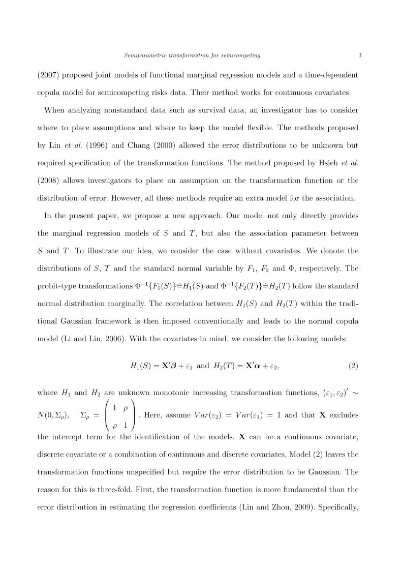
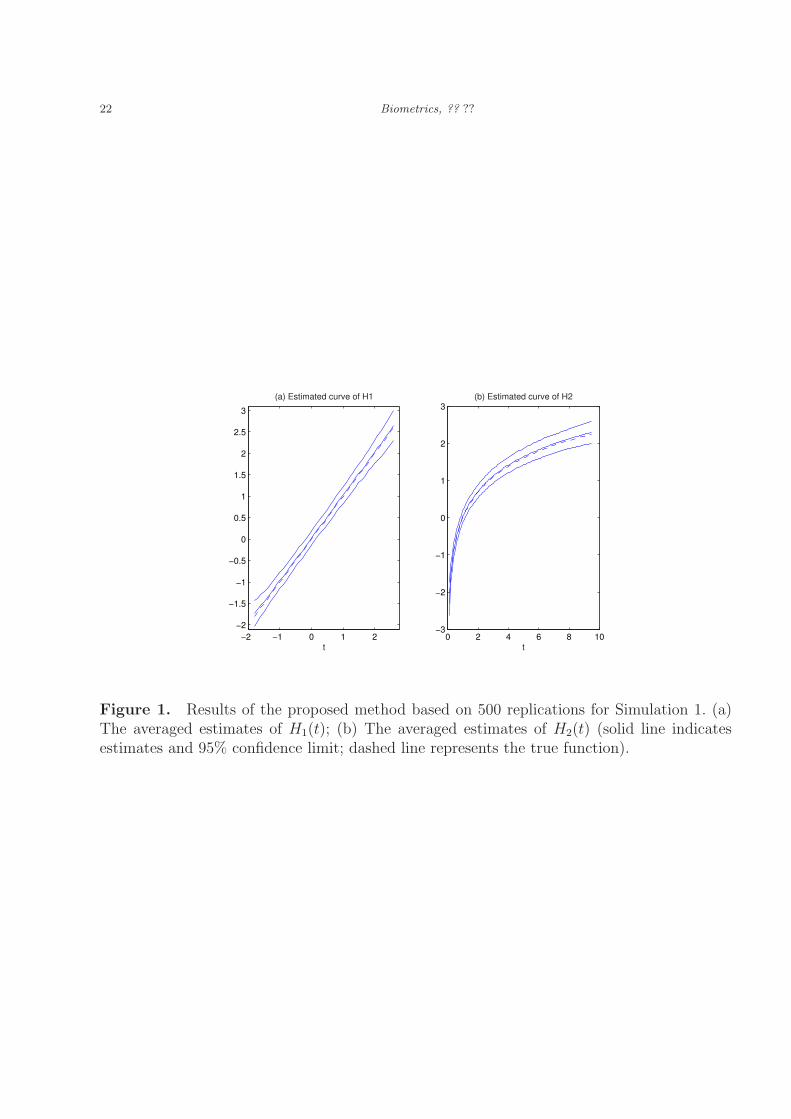
Figures 1(a) and 1(b) display the average of the estimated transformation functions and

their pointwise 95% confidential intervals, which suggest that the proposed method produces

reasonable estimates of the transformation functions.

[Figure 1 about here.]


Simulation 2. Simulation 1 shows that the misspecification of the transformation function

will lead to a seriously biased estimator for the BLSR method. Our method requires the

specification of the error distribution. A natural question is whether the proposed method

is sensitive to the error distribution. To investigate the issue, we generate data similar to

those in Simulation 1, except that the errors (ε1, ε2)′ jointly follow a Clayton copular model

as Pr(ε1 > x, ε2 > y) = φ−1γ [φγ{Pr(ε1 > x)}+ φγ{Pr(ε2 > y)}] with φγ(υ) = (υ−γ − 1)/γ,

γ = 0.5, and both marginal distributions of ε1 and ε2 follow the chi-square distribution with

one degree of freedom. Therefore, the assumption on the error distribution required by our

method is not satisfied, but it follows the requirement of Hsieh, Wang and Ding (2008).

For each set of simulated data, we estimate β, α and the association parameter using the

proposed method, the CBLSR method, the MBLSR method, the CRC1 method and the CRC2

method. The CRC1 method is the CRC method with the transformation function correctly

specified but the error distribution unspecified, and the CRC2 method is the CRC method

with the error distribution correctly specified but the transformation function unspecified. The

transformation functions are misspecified as H1(t) = H2(t) = t in the MBLSR method. Table

2 presents the bias, the SD and the RMSE of β, α and the association parameter. From Table

2, one can see that our estimator is slightly biased due to the misspecification of the error

distribution, while the MBLSR estimator is seriously biased and inefficient. This result implies

that the estimation of the effect of covariates is driven more by the assumptions about the

form of the transformation function than those about the error distribution. The conclusion

is consistent with that founded by Lin and Zhou (2009).


To further investigate the robustness of the proposed method, we also conduct the simulation

studies with γ varying from 0.01 to 10. The resulting estimators are displayed in Table 3.


From Table 3, one can see that the proposed method has a slight bias when γ is small and

essentially no bias for the other case, suggesting that our method is quite robust to the normal

assumption. This occurs probably because the transformation function is nonparametric and

the normal assumption is fairly robust toward some departure (Hanley, 1988).


We also have conducted further simulation studies (denoted as Simulations 3 and 4) to assess

the performance of the proposed method when covariates are continuous and to investigate the

possible loss due to the using of the estimating equations instead of the maximum likelihood

function for the transformation function. The results are reported in the Supplementary

Materials C and D and point to the good performance of the proposed method and hint

at the appropriateness of data analysis reported in the next section.

6. Analysis of a Multiple Myeloma Trial

The motivating example is a trial involving patients with multiple myeloma, a progressive

hematological disease that represents more than 10% of all hematologic cancers. Time to

disease progression and overall survival are often the two main clinical outcomes of mutiple

myeloma patients, whose overall survival or time-to-disease progression ranges from a few

months to more than ten years (Decaux et al., 2008). In an effort to understand the efficicacy

of treatment and the clinical heterogeneities among cancer patients, a total of 264 advanced

multiple myeloma patients were recruited in a randomized study, wherein patients were

randomly assigned to either receive proteasome inhibitor bortezomib (experimental arm) or

high-dose dexamethasone (control arm). A number of clinical and laboratory features that may

provide prognostic information, including age, gender, tumore proliferative index, albumin and

Myeloma score (expression of myeloma markers), were also collected in the study. The purpose

of the analysis is to disclose the relationship between disease progression and overall survival,

and their respective relationships with the treatment and these potential prognostic factors.


In this study, overall survival was assessed from the date patients received their first dose of

study drug to death or censoring, whichever comes first. Time to progression was assessed from

the same starting date to disease progression, which can be censored by death. Hence, overall

survival (T ) and time to progression (S) are two semicompeting outcomes, as the former can

censor the latter, but not vice versa. During the course of the clinical trial, patients’ median

follow-up time was 447 days, and 169 disease progressions and 145 deaths were observed. We

consider the following model: H1(S) = X′β + ε1, and H2(T ) = X′α + ε2, where the covariate

vector X includes treatment status (0=control, 1=experiment), gender (0=male, 1=female),

Myeloma score, tumor proliferative index, age and albumin. Except for treatment status and

gender, all covariates are continuous. The resulting estimates of the regression coefficients

and association parameter and their standard errors are listed in Table 4. We calculated the

standard errors via the resampling method described in Section 3, with 400 bootstrap samples.

We chose 400 as the sample size by monitoring the stability of the standard errors.


Our analysis provides several interesting results. First, Figure 2 depicting the estimated

H1, H2 suggestes that the form of the transformation functions resembles that of a log function.

Hence, the semiparametric transformation models developed for our data can roughly be

interpreted as accelerated failure time models. Second, the prognostic factors act differently on

the two main endpoints. Specifically, treatment status and age have significant effects on time

to progression, but their effects on overall survival are not significant. This suggests that the

treatment and age have only short-term effects on patients’ outcome, with no long-term effect

on patients’ overall survival. On the other hand, the tumor proliferative index and myeloma

score have significant effects for overall survival but not for time to progression, which suggests

that these two prognostic factors have long-term effects on patients’ outcomes, although their

short-term effect is not significant. It is worth noting that albumin is has an effect on both


short- and long-term outcomes, whereas gender is not significant for either outcome. Third,

as measured by the correlation parameter, the two outcomes—time to progression and overall

survival–are correlated even after controlling for the aforementioned prognostic factors. This

hints that, for multiple myeloma, disease progression can indeed be regarded as a precursor or

a surrogate for death. Such information would be helpful for designing next generation therapy

for multiple myeloma patients. Finally, from the resulting estimators, the proportion of the

treatment effect explained by the disease progression, is estimated as P TE = ρβ1/α1 = 1.0678

and its 95% confidence interval is [−1.4117, 3.5473]. The relative effect of treatment effect is

estimated as RE = β1/α1 = 2.7689 and its 95% confidence interval is [−0.4558, 5.9937]. Both

confidence intervals contain zero, implying that disease progression is not a surrogate for death

if the treatment is of interest.

[Figure 2 about here.]

Finally, we propose a procedure to check the validity of the assumed semiparametric trans-

formation models. First, we randomly divided the data into five subsets of equal size. We use

four of the subsets as the training set; the remaining set is used for validation. For each subject

in the validation set, we predicted the subject’s event number of a landmark event and death

up to time t by ENi(t) = − ∫ tt0

Yi(t)d log{Sρ

(H1(t)−X′

iβ, H2(t)−X′iα

)}and

EN2i(t) = − ∫ tt0

Y2i(t)d log(1− Φ

(H2(t)−X′

iα))

, respectively. We investigated the perfor-

mance of the model by examining the prediction error: PE1i =∫ τt0

(Ni(t)− ENi(t)

)d {∑n

k=1 Nk(t)} ,

PE2i =∫ τt0

(N2i(t)− EN2i(t)

)d {∑n

k=1 N2k(t)} . Figures 3 and 4 (in the Supplementary Ma-

terial E) plot the prediction error against the covariates, suggesting that the prediction error

is independent of the covariates—that is, the proposed model basically picks up all of the

covariates’ information, and so the proposed model (2) is reasonable.


7. Discussion

In the current paper, we propose semiparametric transformation models for semicompeting

risk data. Our models allow the transformation function to be unknown, but the error distri-

bution is specified to be normal. In this way, our model can provide direct estimators of the

regression analysis and the association parameter. A simple algorithm is provided to estimate

the transformation functions, and the proposed estimators are shown to be consistent and

asymptotically normal. The simulation studies reveal that our method works well compared

with existing methods.

Acknowledgements

Dr. Lin’s research is supported by the Chinese Natural Science Foundation (11125104) and

the Fundamental Research Funds for the Central Universities.

Supplementary Materials

The appendices referenced in Sections 3, 5 and 6, the code and the data are available with

this article at the Biometrics website on Wiley Online Library.

References

Andersen, E. W. (2005). Two-stage estimation in copula models used in family studies.

Lifetime Data Analysis 11, 333-350.

Buyse, M. and Molenberghs, G. (1998). Criteria for the validation of surrogate endpoints in

randomized experiments. Biometrics 54, 1014–1029.

Chang, S. H. (2000). A two-sample comparison for multiple ordered event data. Biometrics

56, 183–189.

Chen, K., Jin, Z., and Ying, Z. (2002). Semiparametric analysis of transformation models with

censored data. Biometrika 89, 659–668.

Day R., Bryant J., and Lefkopoulou M. (1997). Adaptation of bivariate frailty models for


prediction, with application to biological markers as prognostic indicators. Biometrika 84,

45–56.

Decaux, O., Lode, L., et al. (2008). Prediction of Survival in Multiple Myeloma Based on

Gene Expression Profiles Reveals Cell Cycle and Chromosomal Instability Signatures in

High-Risk Patients and Hyperdiploid Signatures in Low-Risk Patients: A Study of the

Intergroupe Francophone du Myelome. J Clin Oncol 26, 4798–4805.

Ellenberg, S. S. and Hamilton, J.M. (1989). Surrogate endpoints in clinical trials: cancer.

Statistics in Medicine 8, 405–413.

Fine, J. P., Jiang, H. and Chappell, R. (2001). On semi-competing risks data. Biometrika 88,

907–919.

Fleming, T. R. and Harrington, D. P. (1991). Counting Processes and Survival Analysis. New

York: Wiley.

Freedman, L. S., Graubard, B. I., and Schatzkin, A. (1992). Statistical validation of interme-

diate endpoints for chronic disease. Statistics in Medicine 11, 167–178.

Ghosh, D. and Lin, D. Y. (2003). Semiparametric analysis of recurrent events data in the

presence of dependent censoring. Biometrics 59, 877–885.

Ghosh, D. (2009). On Assessing Surrogacy in a Single Trial Setting Using a Semicompeting

Risks Paradigm. Biometrics 65, 521–529.

Hsieh, J., Wang, W. and Ding, A. (2008). Regression analysis based on semicompeting risks

data. J. R. Statist. Soc. B. 70, 3–20.

Jin, Z., Ying, Z,. and Wei, L. J. (2001). A simple Resampling Method by Perturbing the

Minimand. Biometrika 88, 381–390.

Li, Y. and Lin, X. (2006). Semiparametric Normal Transformation Models for Spatially

Correlated Survival Data. Journal of the American Statistical Association 101, 591–603.

Lin, D. Y., Fleming, T. R., and DeGruttola, V. (1997). Estimating the proportion of treatment


effect explained by a surrogate marker. Statistics in Medicine 16, 1515– 1527.

Lin, D. Y., Robins, J. M., and Wei L. J. (1996). Comparing two failure time distributions in

the presence of dependent censoring. Biometrika 83, 381–393.

Lin, D.Y. and Ying, Z. (2003). Semiparametric regression analysis of longitudinal data with

informative drop-outs. Biostatistics 4, 385–398.

Lin, H. Z., YIP, S.F. P. and Chen, F. (2009). Estimating the Population Size for a Multiple

List Problem with an Open Population, Statistica Sinica 19, 177-196.

Lin, H. Z. and Zhou, X. H. (2009). A semi-parametric two-part mixed-effects heteroscedastic

transformation model for correlated right-skewed semi-continuous data. Biostatistics 10,

640–658.

Oakes, D. (1986). Semiparametric Inference in a Model for Association in Bivariate Survival

Data. Biometrika 73, 353–361.

Olsen, M. K. and Schafer, J. (2001). A two-part random-effects model for semi-continuous

longitudinal data. Journal of the American Statistical Association 96, 730–745.

Peng, L. and Fine, J. P. (2006). Nonparametric estimation with left-truncated semicompeting

risks data. Biometrika 93, 367–383.

Peng, L. and Fine, J. P. (2007). Regression Modeling of Semicompeting Risks Data. Biometrics

63, 96–108.

Prentice, R. L. (1989). Surrogate endpoints in clinical trials: Definition and operational criteria.

Statistics in Medicine 8, 431–440.

Wang W. (2003). Estimating the association parameter for copula models under dependent

censoring. J. Roy. Statist. Soc. B. 65, 257–273.

Zhou, X. H., Lin, H. Z and Johnson, E. (2009). Nonparametric heteroscedastic transformation

regression models for skewed data with an application to health care costs. Journal of the

Royal Statistical Society: Series B (Statistical Methodology) 70, 1029–1047.


Received ?? ??. Revised ?? ??. Accepted ?? ??.


−2 −1 0 1 2−2

−1.5

−1

−0.5

0

0.5

1

1.5

2

2.5

3

(a) Estimated curve of H1

t0 2 4 6 8 10

−3

−2

−1

0

1

2

3(b) Estimated curve of H2

t

Figure 1. Results of the proposed method based on 500 replications for Simulation 1. (a)The averaged estimates of H1(t); (b) The averaged estimates of H2(t) (solid line indicatesestimates and 95% confidence limit; dashed line represents the true function).


0 200 400 600 800

02

46

810

Estimated Curve of H1

S(days)

H1(

S)

200 400 600 800 1000

−20

24

6

Estimated Curve of H2

T(days)

H2(

T)

Figure 2. The proposed estimators of H1 and H2 for the myeloma data (solid line: estimated;dotted line: 95% confidence limit).


Table 1The bias, empirical standard deviation (SD), root of mean square error (RMSE) and the empirical coverage

probabilities (CP) of 95% confidence intervals of estimators based on 500 replications using the proposed, the CBLSRand MBLSR methods for Simulation 1.

α βMethod Bias SD RMSE CP Bias SD RMSE CP

Proposed 0.0260 0.1183 0.1211 0.950 0.0277 0.1187 0.1219 0.945CBLSR 0.0090 0.1157 0.1160 0.0063 0.1144 0.1146MBLSR 1.3461 0.3558 1.3923 0.1711 0.1341 0.2174

ρProposed 0.0086 0.0441 0.0449 0.950


Table 2The bias, SD and RMSE of estimators based on 500 replications using the proposed, CBLSR, MBLSR, CRC1 and

CRC2 methods for Simulation 2.

β αMethod Bias SD RMSE Bias SD RMSE

Proposed -0.0846 0.1064 0.1359 -0.0399 0.0994 0.1071CBLSR 0.0047 0.0820 0.0821 0.0071 0.0845 0.0848MBLSR -0.0855 0.1320 0.1573 -2.0418 0.6230 2.1347CRC1 0.0645 0.0863 0.1077CRC2 0.0512 0.0701 0.0868


Table 3The bias, SD and RMSE of estimators using the proposed method with different γ for Simulation 2.

α βγ Bias SD RMSE Bias SD RMSE

0.01 -0.0279 0.0999 0.1037 -0.1197 0.1100 0.16260.1 -0.0277 0.1000 0.1038 -0.1058 0.1085 0.15150.5 -0.0243 0.1005 0.1034 -0.0677 0.1054 0.12531 -0.0349 0.1008 0.1067 -0.0542 0.1041 0.11742 -0.0530 0.1026 0.1155 -0.0465 0.1038 0.11374 -0.0395 0.1004 0.1079 -0.0307 0.0996 0.104210 -0.0344 0.1008 0.1065 -0.0264 0.1002 0.1036


Table 4The estimates from the proposed method for the myeloma data.

α βEstimator SD P-value Estimator SD P-value

Treatment 0.185 0.203 0.363 0.511 0.223 0.022Gender 0.064 0.160 0.689 -0.012 0.194 0.949Score -0.018 0.006 0.007 -0.004 0.008 0.603Index -0.439 0.190 0.021 -0.333 0.242 0.169Age 0.018 0.014 0.189 0.033 0.014 0.015Albumin 0.083 0.017 0.000 0.077 0.019 0.000

ρ0.386 0.077 0.000

semiparametric transformation models for …yili/semicompeting_03_31_2014.pdfbiometrics ??, 1{21...

Documents