senior science tool kit - wikispaces science toolkit... · 2.2 measurements and uncertainty 11 ......
TRANSCRIPT

Senior Science Tool Kit
Measurement & Mathematics
Revision 3 – 2007
Mr. D.J. Young

Table of Contents
Section Title Page
1.0 Orders of Magnitude 1 1.1 Expressing Orders of Magnitude – Scientific Notation 2 1.2 Order of Magnitude Estimates 4 1.3 Powers of 10 and the SI System of Measurement 6 2.0 Measurement Skills 9 2.1 Significant Figures 9 2.2 Measurements and Uncertainty 11 2.3 Estimating Uncertainty 12 2.4 Representing Uncertainty 16 2.5 Calculations with Significant Figures 17 3.0 Precision and Accuracy 19 3.1 Errors in Data 21 3.2 Comparing Values in Science 22 4.0 Mathematical Skills 24 4.1 Dimensional Analysis 26 4.2 Factor Label Method 26 5.0 Dealing with Uncertainties 28 5.1 Error Propagation – Uncertainty in Calculated Results 28
Addition and Subtraction 29 Multiplication and Division 29 Exponents and Square Roots 30 Pure Numbers 31 Uncertainty in a Calculated Mean 31 Uncertainty in the Slope of a Line 32
Appendix Solutions to Worksheets 36

ISB SCIENCE
Science Toolkit Part 1 – Measurement & Mathematics 1.
1.0 Orders of Magnitude Study in science deals with both very large and very small numbers.
The order of magnitude of a number is the power of 10 that is closest to the numerical value of a measurement or quantity.
Order of magnitude is closely related to scientific notation (reviewed in the following section) as a change of one order of magnitude is the same as multiplying or dividing a number by 10. For example 3452 is one order of magnitude larger than 345.2 and two orders of magnitude larger than 34.52. The difference between two quantities in orders of magnitude is basically the difference between the base 10 exponents of the two quantities when written in scientific notation.
For example my mass 8.95×101 kg is roughly 1032 or 32 orders of magnitude larger than
the mass of an electron (9.11×10⁻³¹ kg). That is a big difference! Order of magnitude is important when we consider the range of measurements possible in our physical world i.e.
Object Mass (kg)
Electron 9.11 x 10⁻³¹
Proton 1.67 x 10⁻²⁷
Small coin 1.13 x 10⁻³
Mr. Y. 8.95 x 101
Moon 7.35 x 10²²
Sun 1.99 x 1030
Order of magnitude is useful when approaching problems. Science involves numbers (lots of them) and frequent calculations. When you solve a problem, you can estimate your answer to the nearest power of 10, and compare to the solution you have obtained. If the solution differs by a couple of orders of magnitude you have probably made an error (using the calculator, or perhaps a unit conversion mistake or omission). Careless mistakes!?!?!? Example number 1
Suppose you just calculated the density of vegetable oil from lab data to be 9250 g/mL. How do you know this is wrong? What is the most likely error?
Careless mistakes!?!?!? Example number 2
I just calculated the final velocity for a proton that has been accelerated through an electric field. The calculated velocity is 3.45 x10¹² ms-1. Is this value realistic?

ISB SCIENCE
Science Toolkit Part 1 – Measurement & Mathematics 2.
Careless mistakes!?!?!? Example number 3
Check out this answer to a past exam question:
Clearly 7.7 × 10¹² kg is unreasonable.
1.1 Expressing Orders of Magnitude: Scientific Notation Consider the following definition: “One light year is the distance that light travels (in a vacuum) in one year”. Given that the speed of light in a vacuum is about 300 million meters per second, calculate the length of a light year in meters? (see below for answer)
You will no doubt realize that it is convenient to express your answer in scientific notation (ie. it is a really big number). Frequently in physics, very large and very small numbers are expressed in scientific notation. Scientific notation is used to when expressing numbers to the correct number of significant figures and can also make unit conversions quite easy.
You must be comfortable with scientific notation and recognizing
powers of 10. You must be able to enter these numbers in your
calculator correctly if you are to succeed in science courses.
General form for scientific notation is:
M x 10N
Where 1 < M < 10 and N is an integer
[a light year is 9.46 ×××× 1015 m]

ISB SCIENCE
Science Toolkit Part 1 – Measurement & Mathematics 3.
Practice Worksheet 1.1 – Scientific Notation Review Express the following measurements in scientific notation: a) 36800 g
b) 0.031 J c) 101 V
d) 0.0000000405 s e) 26010000000 cm f) 0.000032 m3
Rewrite the following numbers in standard notation: g) 2.74×10⁻⁴
h) 6.792×10² i) 5.209×10⁶
j) 4.91×10⁻⁹ k) 3.81×100 l) 7.29×101
Estimate answers to the following and then evaluate using your calculator. Express the solutions using correct scientific notation: m) n) Estimate: Estimate: Actual: Actual: o)
Estimate: Actual:
3
12
10781.4
10321.8
××
13
5 3 5
22
5.55 10(3.78 10 ) (4.10 10 )
2.73 10
−−
×× × × ×
×
( )23
16
3
8.45 102.04 10
5.75 10
−−
×× ×
×

ISB SCIENCE
Science Toolkit Part 1 – Measurement & Mathematics 4.
1.2 Order of Magnitude Estimates
Fermi's piano tuner problem and other back of envelope estimates
Enrico Fermi designed the first nuclear reactor to achieve a fission chain reaction. As a professor at the University of Chicago, Fermi would challenge his students to solve problems that seemed impossible due to lack of given information. Fermi wanted his students to develop their abilities to make assumptions and estimations and work out rough solutions on the back of an old envelope rather than making detailed (with calculators in your case) calculations. A typical Fermi problem is to determine the number of piano tuners in Chicago given only the population of the city.
Fermi’s solution:
1. Given Chicago has a population of about 3 million people. 2. Assume that the average family has four members so that the number of families in
Chicago must be about 750,000. 3. Assume one out of five families owns a piano, there will be 150,000 pianos in
Chicago. 4. If the average piano tuner worked 5 days a week tuning 4 pianos each day and had a
two week vacation during the summer…. 5. In one year (50 weeks) he would tune 1,000 pianos. Therefore there must be about
150 piano tuners in Chicago.
This method is not guaranteed correct but it is a valid first estimate that might be off by no more than a factor of 2 or 3 but will definitely not inaccurate by an order of magnitude (we should not expect 15 piano tuners, or 1,500 piano tuners).
Solving Fermi problems develop critical skills that lead to success in science
• Fermi questions provide limited information and require assumptions
• Fermi questions require students to ask and answer further questions
• Fermi questions demand estimations often of common everyday values like the mass of a brick or the length of a soccer field.
• Fermi questions emphasize process rather than product

ISB SCIENCE
Science Toolkit Part 1 – Measurement & Mathematics 5.
Practice Worksheet 1.2 – Fermi Problems Strategies
“everything should be made as simple as possible, but no simpler” Einstein. Don’t make numbers more precise than necessary
• Round to the nearest 0, 5 or 10
• Don’t worry about numbers like π (call it 3 .. or even 2) Guess numbers that you don’t know
• Try to use common sense to make good guesses
• Accurate guesses requires experienced common sense … this comes from education …. pay attention
Make complicated geometry simple
• Assume the cow is a sphere Extrapolate from what you do know
• Use ratios
• Use known similar values (for example you could reasonably assume the density of gasoline is 1 g/mL)
Example Fermi questions for you to try
1. How many jelly beans fill a one litre jar?
2. What is the mass of the entire student body of the school?
3. How many water balloons would it take to fill the school gymnasium?
4. How many tennis balls would cover the area of two tennis courts?
5. How high would a pile of one trillion 1 dollar bills reach?
6. How much gasoline is used by all the cars in China in one year?

ISB SCIENCE
Science Toolkit Part 1 – Measurement & Mathematics 6.
1.3 Powers of 10 and the SI System of Measurement The SI System of Measurement
• SI units (Le Systeme International d’Unites) – or more commonly called the metric system.
• Adopted for scientific research in 1960 worldwide, used as general measurement in most countries (USA and UK excepted)
Fundamental SI Units
• cannot be measured in simpler form
• you must know these basic quantities (and generally you need to convert them to solve problems)
Quantity Fundamental
SI unit SI symbol
Length Meter m
Mass Kilogram kg
Time Second s
Electric Current Ampere A
Absolute Temperature Kelvin K
Amount of Substance Mole mol
• some quantities are based on the measurement of two or more fundamental quantities – units for these are called derived units - a common example would be velocity (ms-1)
• note that the IBO accepted format for the velocity unit is ms-1 and not m/s. This applies to all derived units. (Get used to it!)
• the fundamental SI units are based on standards ex. the standard kilogram is a platinum-iridium cylinder kept in France, a standard second is the time for 9 192 631 770 vibrations of a cesium atom.
ISB SCIENCE
Science Toolkit Part 1 – Measurement & Mathematics 7.
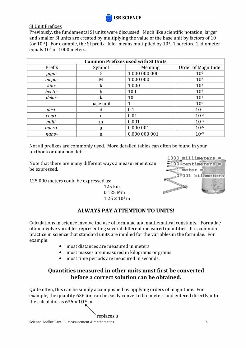
SI Unit Prefixes Previously, the fundamental SI units were discussed. Much like scientific notation, larger and smaller SI units are created by multiplying the value of the base unit by factors of 10 (or 10-1). For example, the SI prefix “kilo” means multiplied by 103. Therefore 1 kilometer equals 103 or 1000 meters.
Common Prefixes used with SI Units
Prefix Symbol Meaning Order of Magnitude
giga- G 1 000 000 000 109
mega- M 1 000 000 106
kilo- k 1 000 103
hecto- h 100 102
deka- da 10 101
base unit 1 100
deci- d 0.1 10-1
centi- c 0.01 10-2
milli- m 0.001 10-3
micro- µ 0.000 001 10-6
nano- n 0.000 000 001 10-9
Not all prefixes are commonly used. More detailed tables can often be found in your textbook or data booklets.
Note that there are many different ways a measurement can be expressed. 125 000 meters could be expressed as:
125 km 0.125 Mm
1.25 × 10⁵ m
ALWAYS PAY ATTENTION TO UNITS! Calculations in science involve the use of formulae and mathematical constants. Formulae often involve variables representing several different measured quantities. It is common practice in science that standard units are implied for the variables in the formulae. For example:
• most distances are measured in meters
• most masses are measured in kilograms or grams
• most time periods are measured in seconds.
Quantities measured in other units must first be converted
before a correct solution can be obtained. Quite often, this can be simply accomplished by applying orders of magnitude. For
example, the quantity 636 µm can be easily converted to meters and entered directly into
the calculator as 636 ×××× 10-6 m.
replaces µ

ISB SCIENCE
Science Toolkit Part 1 – Measurement & Mathematics 8.
Practice Worksheet 1.3 – SI Prefixes
Rewrite the following measurements using appropriate metric prefixes. There could be more than one reasonable answer for some questions. a) 1.89 × 10⁹ m b) 0.004 L
c) 360000 g d) 4.5 × 10⁻² m
e) 1.27 × 10⁻⁸ s f) 0.00057 kg
g) 0.00247 A
h) 0.45 m
Write the following in base units (use scientific notation if appropriate) i) 1.87 Gg j) 63 µm
k) 5 cs l) 0.98 km
m) 4.5 mA n) 9230 nm
o) 0.654 km p) 0.78 mg
ISB SCIENCE
Science Toolkit Part 1 – Measurement & Mathematics 9.
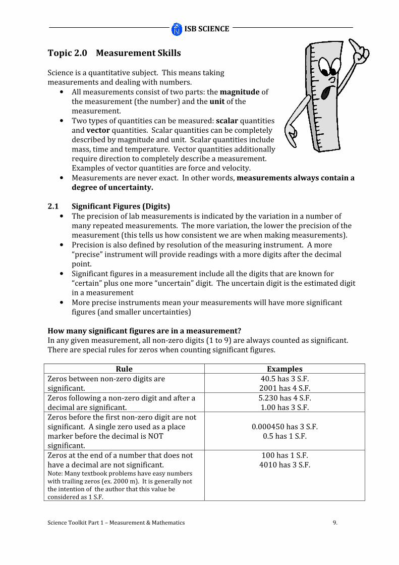
Topic 2.0 Measurement Skills Science is a quantitative subject. This means taking measurements and dealing with numbers.
• All measurements consist of two parts: the magnitude of the measurement (the number) and the unit of the measurement.
• Two types of quantities can be measured: scalar quantities and vector quantities. Scalar quantities can be completely described by magnitude and unit. Scalar quantities include mass, time and temperature. Vector quantities additionally require direction to completely describe a measurement. Examples of vector quantities are force and velocity.
• Measurements are never exact. In other words, measurements always contain a
degree of uncertainty. 2.1 Significant Figures (Digits)
• The precision of lab measurements is indicated by the variation in a number of many repeated measurements. The more variation, the lower the precision of the measurement (this tells us how consistent we are when making measurements).
• Precision is also defined by resolution of the measuring instrument. A more “precise” instrument will provide readings with a more digits after the decimal point.
• Significant figures in a measurement include all the digits that are known for “certain” plus one more “uncertain” digit. The uncertain digit is the estimated digit in a measurement
• More precise instruments mean your measurements will have more significant figures (and smaller uncertainties)
How many significant figures are in a measurement?
In any given measurement, all non-zero digits (1 to 9) are always counted as significant. There are special rules for zeros when counting significant figures.
Rule Examples
Zeros between non-zero digits are significant.
40.5 has 3 S.F. 2001 has 4 S.F.
Zeros following a non-zero digit and after a decimal are significant.
5.230 has 4 S.F. 1.00 has 3 S.F.
Zeros before the first non-zero digit are not significant. A single zero used as a place marker before the decimal is NOT significant.
0.000450 has 3 S.F.
0.5 has 1 S.F.
Zeros at the end of a number that does not have a decimal are not significant. Note: Many textbook problems have easy numbers with trailing zeros (ex. 2000 m). It is generally not the intention of the author that this value be considered as 1 S.F.
100 has 1 S.F. 4010 has 3 S.F.

ISB SCIENCE
Science Toolkit Part 1 – Measurement & Mathematics 10.
Practice Worksheet 2.1 – Significant Figures 1. How many significant figures are there in each measurement? a) 727.2 m b) 601 g c) 46.0 mL d)0.044 g
e) 320 cm f) 0.00401 L g) 1060 s h) 123456 mg
i) 12.500 g j) 340.010 mL k) 0.02 m l) 0.5 kg
m) 1.113 × 10³ kg
n)8.00 × 10⁸ m o) 6.80 °C p)7.67 × 101 °C
2. Write the following measurements to the number of significant figures listed
a. 654.64587 m to 6 SF
b. 654.64587 m to 3 SF
c. 654.64587 m to 1 SF
d. 100 cm to 3 SF
e. 7000 cm to 2 SF
f. 125000 mm to 4 SF

ISB SCIENCE
Science Toolkit Part 1 – Measurement & Mathematics 11.
2.2 Measurements and Uncertainty How long is the pencil?
2 3 4 5 When making measurements, the last digit of the measurement is always an estimate. This digit is called the uncertain digit (because it is an estimate). When taking a measurement:
• read the scale to the smallest graduation (the limit of measurement)
• estimate the next digit of the measurement This produces a more precise measurement but with a degree of uncertainty. When deciding on a reasonable uncertainty in a measurement, one must consider the instrument itself AND how the measurement is made. A general starting point for an uncertainty determination is:
A rule of thumb: The degree of
uncertainty is at a minimum equal to
half of the smallest graduation on the
measurement scale and is often
greater.
Uncertainty and error are two very different concepts. An error in measurement is how far the measured quantity is from the actual value. Errors are not part of measurement uncertainty although discussion of errors is important in lab reporting. The quantity of uncertainty reflects the precision of the measuring tool used (for example a 10 mL graduated cylinder is more precise than a 100 mL cylinder) AND any limitations in the measurement technique itself (for example, using a meter stick to measure the rebound height of a bouncing ball). The National Institute of Standards and Technology (NIST) uses the symbol “u” to represent uncertainty. For a temperature measurement, the uncertainty would be represented as “uT”.
?
ISB SCIENCE
Science Toolkit Part 1 – Measurement & Mathematics 12.
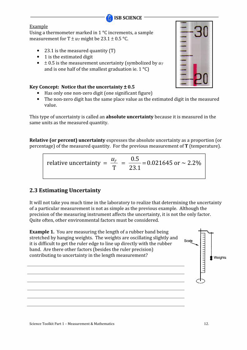
Example
Using a thermometer marked in 1 °C increments, a sample
measurement for T ± uT might be 23.1 ± 0.5 °C.
• 23.1 is the measured quantity (T)
• 1 is the estimated digit
• ± 0.5 is the measurement uncertainty (symbolized by uT
and is one half of the smallest graduation ie. 1 °C)
Key Concept: Notice that the uncertainty ±±±± 0.5
• Has only one non-zero digit (one significant figure)
• The non-zero digit has the same place value as the estimated digit in the measured value.
This type of uncertainty is called an absolute uncertainty because it is measured in the same units as the measured quantity.
Relative (or percent) uncertainty expresses the absolute uncertainty as a proportion (or percentage) of the measured quantity. For the previous measurement of T (temperature).
2.3 Estimating Uncertainty It will not take you much time in the laboratory to realize that determining the uncertainty of a particular measurement is not as simple as the previous example. Although the precision of the measuring instrument affects the uncertainty, it is not the only factor. Quite often, other environmental factors must be considered. Example 1. You are measuring the length of a rubber band being stretched by hanging weights. The weights are oscillating slightly and it is difficult to get the ruler edge to line up directly with the rubber band. Are there other factors (besides the ruler precision) contributing to uncertainty in the length measurement?
0.5relative uncertainty 0.021645 or ~ 2.2%
T 23.1
Tu= = =
ISB SCIENCE
Science Toolkit Part 1 – Measurement & Mathematics 13.
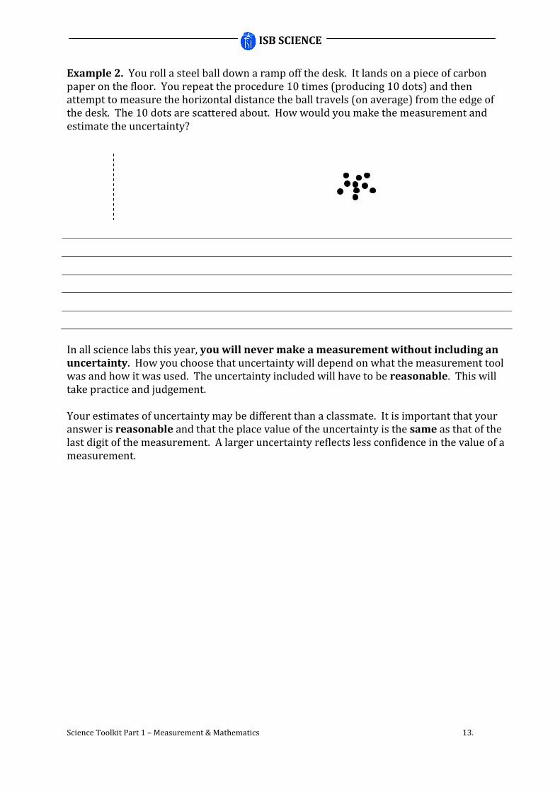
Example 2. You roll a steel ball down a ramp off the desk. It lands on a piece of carbon paper on the floor. You repeat the procedure 10 times (producing 10 dots) and then attempt to measure the horizontal distance the ball travels (on average) from the edge of the desk. The 10 dots are scattered about. How would you make the measurement and estimate the uncertainty?
In all science labs this year, you will never make a measurement without including an
uncertainty. How you choose that uncertainty will depend on what the measurement tool was and how it was used. The uncertainty included will have to be reasonable. This will take practice and judgement. Your estimates of uncertainty may be different than a classmate. It is important that your answer is reasonable and that the place value of the uncertainty is the same as that of the last digit of the measurement. A larger uncertainty reflects less confidence in the value of a measurement.

ISB SCIENCE
Science Toolkit Part 1 – Measurement & Mathematics 14.
Practice Worksheet 2.3 – Estimating Uncertainty Make measurements for each of the situations shown in the diagrams. Include uncertainty with each measurement.
Example 1. Measure the volume in each of the three
pipettes shown.
From left to right:
Pipette 1 : 5.75 ± 0.05 mL
Pipette 2 : 3.0 ± 0.3 mL
Pipette 3 : 0.35 ± 0.05 mL All are acceptable measurements.
Example 2. What is the diameter of this penny?
Answer: Around 1.9 ± 0.2 cm This is not a realistic measurement because in the lab the ruler would be placed across the penny. The diagram does not allow that so the uncertainty is more conservative.
Cylinder 1 Cylinder 2 Cylinder 3

ISB SCIENCE
Science Toolkit Part 1 – Measurement & Mathematics 15.
Burette 1 (initial volume) Burette 2 (final volume)
Temperature 1 Length 1 (scale in cm) Voltage 1
Length 2
Mass 1 Length 3 (scale in cm)

ISB SCIENCE
Science Toolkit Part 1 – Measurement & Mathematics 16.
2.4 Representing uncertainty Tables Uncertainty should be included in the table column headings with units. Example 1
Velocity
/ ± 0.3 ms-1
4.6
5.9
7.4
Example 2 (uncertainties of calculated values may not always be the same)
Velocity / ms-1
4.6 ± 0.2
5.9 ± 0.3
7.4 ± 0.4
Graphs Measurement uncertainty is shown graphically using uncertainty bars.
The data point is a small dot that has been circled. The uncertainty bars show that the point could reasonably be anywhere inside the shaded rectangle. The uncertainty is also noted on the axis label with the unit of measurement. On some graphs, the uncertainty bars may be too small to show relative to the graph scale. When this occurs, a note should be added indicating that this is the case.
The backslash is another form of notating units in a table or on a graph. You can also place units in parentheses
Note that the last digit of each measurement and the uncertainty are in the same place value column
ISB SCIENCE
Science Toolkit Part 1 – Measurement & Mathematics 17.
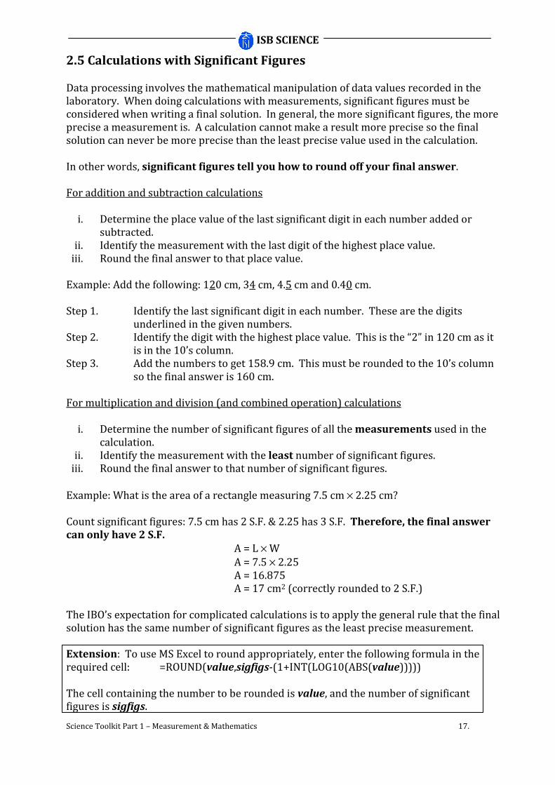
2.5 Calculations with Significant Figures
Data processing involves the mathematical manipulation of data values recorded in the laboratory. When doing calculations with measurements, significant figures must be considered when writing a final solution. In general, the more significant figures, the more precise a measurement is. A calculation cannot make a result more precise so the final solution can never be more precise than the least precise value used in the calculation. In other words, significant figures tell you how to round off your final answer. For addition and subtraction calculations
i. Determine the place value of the last significant digit in each number added or subtracted.
ii. Identify the measurement with the last digit of the highest place value. iii. Round the final answer to that place value.
Example: Add the following: 120 cm, 34 cm, 4.5 cm and 0.40 cm. Step 1. Identify the last significant digit in each number. These are the digits
underlined in the given numbers. Step 2. Identify the digit with the highest place value. This is the “2” in 120 cm as it
is in the 10’s column. Step 3. Add the numbers to get 158.9 cm. This must be rounded to the 10’s column
so the final answer is 160 cm. For multiplication and division (and combined operation) calculations
i. Determine the number of significant figures of all the measurements used in the calculation.
ii. Identify the measurement with the least number of significant figures. iii. Round the final answer to that number of significant figures.
Example: What is the area of a rectangle measuring 7.5 cm × 2.25 cm? Count significant figures: 7.5 cm has 2 S.F. & 2.25 has 3 S.F. Therefore, the final answer
can only have 2 S.F.
A = L × W
A = 7.5 × 2.25 A = 16.875 A = 17 cm2 (correctly rounded to 2 S.F.)
The IBO’s expectation for complicated calculations is to apply the general rule that the final solution has the same number of significant figures as the least precise measurement.
Extension: To use MS Excel to round appropriately, enter the following formula in the required cell: =ROUND(value,sigfigs-(1+INT(LOG10(ABS(value)))))
The cell containing the number to be rounded is value, and the number of significant figures is sigfigs.

ISB SCIENCE
Science Toolkit Part 1 – Measurement & Mathematics 18.
63.45
7.2
(17.3 9.2)
1.25
(77.67 45.786)
9.87231
6.78 2.3 19.3 35.6 14.5 9.87
9
(6.0 56.6) (12.34 4.09)
14.4 (16.9 3.12)
−
×
+ + + + +
+ ×−
×
-3
Do this . .
mD=
V
m 112.5D = =
l×w×h (11.2×2.34×5.21)
D = 0.824 g cm -3
Try to avoid this . .
V = l×w×h = 11.2×2.34×5.21
V = 136.54368
m 112.5D = =
V (136.54368)
D = 0.824 g cm
Practice Worksheet 2.5 – Calculations with Significant Figures Solve the following problems, show complete solutions when formulae or equations apply. Round your answer to the correct number of significant figures, watch for correct units!
a. b. c. d. e.
f. A rock is found to have a volume of 18.65 cm3 and a mass of 56.2 g. Find the density of the rock.
g. A triangle is measured to have a base of 4.5 cm
and a height of 6.05 cm. What is the area of the triangle?
h. A circle has a diameter of 12.3 cm. What is the
area of the circle?
Important notes:
• When performing calculations that have multiple steps, carry all decimals and round off once at the end of the calculation. DO NOT ROUND each calculation.
• It is good practice to rearrange equations and make substitutions so that one overall calculation can be performed on the calculator rather than a series of steps. For example: to determine the density of a 112.5 g block with the following dimensions; length 11.2 cm, width 2.34 cm and height 5.21 cm.
• Many textbooks and worksheets do not consider significant figures when writing sample problems that use easy numbers like 1500 m. In these types of problems, we will consider the trailing zeros (the ones at the end) to be significant. It would be more correct though to use scientific notation or more appropriate units. For example: to properly write 1500 m to show that the last zeros are significant (total 4 S.F.)
ANSWER: 1.500 × 10³ m OR 1.500 km

ISB SCIENCE
Science Toolkit Part 1 – Measurement & Mathematics 19.
3.0 Precision and Accuracy
• Good science involves measuring a physical quantity a number of times.
• We often use the terms precision and accuracy interchangeably when talking about an experimental result. Technically, they mean very different things. Remember this when writing lab reports.
Accuracy is an indication of how close a measurement is to the accepted value. Precision is an indication of the agreement among a number of measurements made in the same way. Alternatively, precision is often used when referring to the resolution of a measuring instrument. We say that instruments that are scaled with small graduations are more precise than those with larger graduations.

ISB SCIENCE
Science Toolkit Part 1 – Measurement & Mathematics 20.
Practice Worksheet 3.0 – Precision and Accuracy
Consider the following table of results for 4 students who are trying to measure “g”, the acceleration of a falling object due to gravity. The accepted value for “g” is 9.81 ms-2. Table 1: Measurements of ‘g’ in Physics class
Trial Bob Joe Sue Kate
1 7.83 9.53 8.70 9.72
2 11.61 9.38 8.75 9.86
3 8.85 8.87 8.77 9.70
Mean 9.43 9.26 8.74 9.76
Compare the accuracy and precision of each student.
Whose results are meaningful, and whose results are questionable?

ISB SCIENCE
Science Toolkit Part 1 – Measurement & Mathematics 21.
3.1 Errors in Data There are three types of errors that can occur when collecting data: Human Errors
Includes the following
• misreading scales
• mistakes copying raw data to final lab report
• not following procedures properly You should be aware of this and act to avoid such errors. This type of error can be mentioned in a lab report to explain a rogue data point or inconsistency. Human errors however SHOULD NOT be the focus of a formal evaluation of procedure and results. Systematic Error
A systematic error is an error that tends to be consistent for all measurements (built in). Reasons include:
• badly made instruments
• poorly calibrated (zero error)
• instrument parallax (reading a scale at an angle)
• limitations of experiment (e.g. friction or air resistance) Systematic errors can often be minimized or corrected before the investigation is carried out. They should definitely be considered when discussing results. The best indication of a systematic error is a y-intercept value appearing on a data plot for the experiment. For this reason alone, never force a graph through the origin – you may be ignoring a
significant error.
Example: In the previous experiment, it is likely that friction would have an effect on the value of “g” calculated in a falling object experiment.
• How would it affect the result?
• Would you see a different effect depending on the object used in the experiment?
ISB SCIENCE
Science Toolkit Part 1 – Measurement & Mathematics 22.
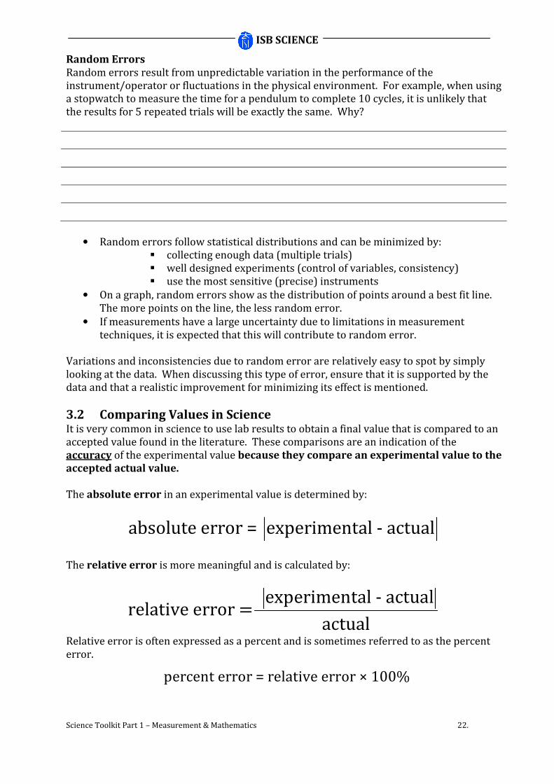
Random Errors
Random errors result from unpredictable variation in the performance of the instrument/operator or fluctuations in the physical environment. For example, when using a stopwatch to measure the time for a pendulum to complete 10 cycles, it is unlikely that the results for 5 repeated trials will be exactly the same. Why?
• Random errors follow statistical distributions and can be minimized by: collecting enough data (multiple trials) well designed experiments (control of variables, consistency) use the most sensitive (precise) instruments
• On a graph, random errors show as the distribution of points around a best fit line. The more points on the line, the less random error.
• If measurements have a large uncertainty due to limitations in measurement techniques, it is expected that this will contribute to random error.
Variations and inconsistencies due to random error are relatively easy to spot by simply looking at the data. When discussing this type of error, ensure that it is supported by the data and that a realistic improvement for minimizing its effect is mentioned.
3.2 Comparing Values in Science It is very common in science to use lab results to obtain a final value that is compared to an accepted value found in the literature. These comparisons are an indication of the accuracy of the experimental value because they compare an experimental value to the
accepted actual value. The absolute error in an experimental value is determined by:
absolute error = experimental - actual
The relative error is more meaningful and is calculated by:
experimental - actualrelative error =
actual
Relative error is often expressed as a percent and is sometimes referred to as the percent error.
percent error = relative error × 100%

ISB SCIENCE
Science Toolkit Part 1 – Measurement & Mathematics 23.
The percent difference is the difference between two calculated or experimental values. You may use this if you wish to compare two measurements of the same quantity but made in different ways.
1 2
value 1 - value 2percent difference =
v +v
2
Sample problem: An experiment was done to calculate the speed of a wave moving along a string. One method produced a value of 13.4 ms-1 while a second different method produces a value of 12.1 ms-1. Determine the percent difference between these two experimental values.
Practice Worksheet 3.2 – Absolute and Percent Errors Consider the following table of results for 4 students who are trying to measure “g”, the acceleration of a falling object due to gravity. The accepted value for “g” is 9.81 ms-2. Table 1: Measurements of ‘g’ in Physics class
Trial Bob Joe Sue Kate
1 7.83 9.53 8.70 9.72
2 11.61 9.38 8.75 9.86
3 8.85 8.87 8.77 9.70
Mean 9.43 9.26 8.74 9.76
Calculate the absolute and percentage error for each student.

ISB SCIENCE
Science Toolkit Part 1 – Measurement & Mathematics 24.
4.0 Mathematical Skills Applying mathematics is a critical aspect of problem solving in science. Many textbooks provide excellent mathematical review sections in the Appendices. Use these to refresh your knowledge or as a quick reference. The basic math skills required for senior science courses are as follows: Arithmetic and Computation
• Make calculations involving addition, subtraction, multiplication and division.
• Recognize and use expressions in decimal and standard form (scientific notation). Make calculations involving numbers in scientific notation.
• Use calculators to evaluate exponents; reciprocals; roots; logarithms to base 10; logarithms to base e; powers; arithmetic means; degrees; radians; quadratic equations; natural sine, cosine and tangent functions and their inverse.
• Express fractions as percentages and vice versa. Algebra
• Change the subject of an equation by manipulation of the terms including integer and fractional indices and square roots.
• Solve simple algebraic equations, and simultaneous linear equations involving two variables.
• Substitute numerical values into algebraic equations.
• Comprehend the meanings of (and use) the symbols /, <, >, ≤, ≥, ±, ≈, ∆x, ∝, x. Geometry and Trigonometry
• Calculate areas of right-angled and isosceles triangles, circumferences and areas of circles, volumes of rectangular blocks, cylinders and spheres, and surface areas of rectangular blocks, cylinders and spheres. Relevant formulas need not be recalled.
• Use Pythagoras’ theorem, similarity of triangles and recall that the angles of a triangle add up to 1800 (and of a rectangle, 3600).
• Understand the relationship between degrees and radians, and translate from one to the other.
• Recall the small angle approximations (tan θ ≅ sin θ for small angles). It is also extremely important that you are familiar with and know how to use your calculator efficiently and correctly. You do not learn how to solve problems by watching the teacher do them. To be successful, you must attack each problem aggressively and do not be afraid to make mistakes.
BRING A CALCULATOR TO EVERY CLASS AND MAKE SURE YOU USE IT TO OBTAIN
THE CORRECT SOLUTION FOR EVERY EXAMPLE PROBLEM WE DO!

ISB SCIENCE
Science Toolkit Part 1 – Measurement & Mathematics 25.
Practice Worksheet 4.0 – Math and Calculator Review Evaluate the following using your calculator. Express your answer with the proper number of significant digits.
a) (386)2 b) √34
c) cos 45o
d) 1/698
e) 0.7247π f) sin-1 0.325
g)
h) i)
Rewrite the following equations for the variable requested
j) solve for V
k) solve for I l) solve for q1
m) solve for di
n) solve for t o) solve for g
12
2
1084
2345637
×
××
.823
8367
001.
.
.=
x
556
337242
.
)( ×−
V
mD =
2
2
1atd =
0
111
ddf i
+=
2
21
r
qqkF =IVP ×=
g
lT π2=

ISB SCIENCE
Science Toolkit Part 1 – Measurement & Mathematics 26.
4.1 Dimensional Analysis The dimension of a measurement refers to its unit. Dimensional analysis means exactly that pay attention to units! This simple example shows the benefit of dimensional analysis. We know that speed is measured in m/s (or ms-1) and that speed is a rate (a measurement of how a quantity changes with time). If a formula for speed was given as:
tv =
d
You might notice something wrong right away just by considering the units involved. Dividing time by distance will not yield the desired unit m/s but rather would produce a quantity with the unit s/m. The formula is therefore incorrect.
4.2 Factor Label Method Factor label method is a technique utilizing dimensional analysis to ensure the math is correct. A conversion factor is an equality statement between two units. For example 1 m = 100 cm and 1 hour = 60 min are both conversion factors (Tip: check out the website for a useful unit conversion program). Factor-label method involves multiplying the value to be converted by appropriate conversion factors written as fractions (which have a value of 1). When arranging conversion factors as fractions, the numerator and denominator are determined by what unit is desired in the final answer and by what unit needs to be cancelled. Example 1: Convert 4.5 m to cm.
Step 1. Determine the required conversion factor: 1 m = 100 cm Step 2. Multiply 4.5 m by the conversion factor written as fraction.
100 cm4.5 m×
1 m “m” cancels leaving “cm” and the answer 450 cm
You may need to multiply by a series of factors to get the conversion you want. Example 2: Convert 1.25 days to seconds
24 hours 60 min 60 s1.25 days × × × = 108000 s
1 day 1 hour 1 min
In this example, days are converted to hours, then hours to minutes, and finally minutes to seconds to get the answer.
Significant figure rules do not apply to unit conversion factors

ISB SCIENCE
Science Toolkit Part 1 – Measurement & Mathematics 27.
Dimensional analysis is a very useful technique that can be applied to help ensure the correct method is used for solving all kinds of problems. Example 3: How many grams of water can be made by the combustion of 4.6 g of
hydrogen gas with excess oxygen according to the equation 2 H2 + O2 2 H2O?
-12 22-1
2
4.6 g H 2 H O × ×18.0 g mol = 41 g H O
2 H2.0 g mol
Practice Worksheet 4.2 – Unit Conversion You may need to look up some unit conversion factors to complete these unit conversion problems:
1. Convert 4.56 L to mL 2. Convert 12400 m to km 3. Convert 35.6 min to seconds 4. Convert 15800 s to hours 5. Convert 85 km to meters 6. Convert 1.2 hours to seconds
7. Convert 1.2×105 mm to meters
8. Convert 8.9×10³ days to minutes 9. Convert 450 g to kilograms 10. Convert 15.6 inches to centimeters 11. Convert 65 kmh-1 to ms-1 12. Convert 25 ms-1 to kmh-1
13. Convert the speed of light (3.0×10⁸ ms-1) to km day-1
14. Convert 565 kPa to atmospheres (atm)
15. Convert 987 ft to meters 16. Convert 123 lbs to kilograms 17. Convert 76 0F to Celsius 18. Convert 28 0C to Kelvin 19. Convert 8763 mL to dm3 20. Convert 1.3 hours to minutes
IN A FAR AWAY GALAXY ON THE PLANET QUAIZZORP
One Nard (Nd) is 8 Quats (Q) long, therefore 1 Nd = 8 Q. A mushy can run 60 Nards in one minute (60 Nd min-1). Answer the following questions in the space provided. Don’t forget units.
1. How many Quats per second can a mushy run?
2. Fred owns a mushy pasture measuring 10.0 Nards by 12 Nards (or 120 Nd2). How many square Quats (Q2) does Fred own?
3. All mushys weigh exactly 12 Zugs. Fred sells 80.2 % of his 150 mushys at a rate of
3.2 $nickers per Zug. How many $nickers did Fred get?
4. Fred’s mushy mashing machine can manage to mash 6.0 mushys in 11 minutes. How many Zugs of mashed mushy can it produce in 1.0 hours?

ISB SCIENCE
Science Toolkit Part 1 – Measurement & Mathematics 28.
5.0 Dealing with Uncertainties Recall, when making measurements:
• every measurement has an uncertainty associated with it
• by convention, the minimum uncertainty usually equals half the limit of the smallest graduation on the scale of the measurement instrument
• the uncertainty is always written with ONE significant digit
• the place setting of the uncertainty matches the place setting of the estimated digit in the measurement
5.1 Error Propagation – Uncertainty in Calculated Results It is quite common to measure two or more quantities (each with their individual uncertainties) and combine the information to calculate a desired value. For example, to find density we may measure mass and volume and then calculate the density using the appropriate equation. The uncertainty in the original mass and volume measurements will propagate to the calculated density value. Consider mass to be 11.4 ± 0.2 g and the volume to be 9.6 ± 0.5 cm3.
Possible maximum density = 11.6 ÷ 9.1 = 1.2747 g cm-3
Actual calculated density value = 11.4 ÷ 9.6 = 1.1875 g cm-3
Possible minimum density = 11.2 ÷ 10.1 = 1.1089 g cm-3
As the calculated result can only have 2 S.F., it would be expressed as 1.2 ± 0.1 g cm-3.
The range of the calculated result is 1.1 to 1.3 g cm-3 and encompasses both the
maximum and minimum possible values.
There are more efficient ways of determining the propagated uncertainty in a calculated result. The method used depends on the type of calculations conducted.
+ 0.0872
- 0.0786

ISB SCIENCE
Science Toolkit Part 1 – Measurement & Mathematics 29.
(X×Y)R=
Z
Addition and Subtraction of Measured Quantities
When adding or subtracting measurements – ADD THE UNCERTAINTIES
Let’s say you make 3 measurements: X ± uX, Y ± uY, and Z ± uZ where uX, uY, and uZ are the absolute uncertainties of the respective measurements. You are required to combine these measurements to obtain the result R using the following formula:
R = X + Y – Z
The absolute uncertainty in R is determined by
uR ≈≈≈≈ uX + uY + uZ
Note the rule for addition or subtraction is the same. ADD the uncertainties. Example 1.
Find the perimeter of a rectangle measuring 5.0 ± 0.5 m by 3.0 ± 0.5 m.
P = (5.0 ± 0.5 m) + (3.0 ± 0.5 m) + (5.0 ± 0.5 m) + (3.0 ± 0.5 m)
P = 16.0 ± 2.0 m
P = 16 ± 2 m (uncertainty must be rounded to one significant figure) We again could look at it in terms of maximum and minimum values for the measurements i.e. maximums 5.5 m and 3.5 m, minimums 4.5 m and 2.5 m. If all the maximum measurements were used in the calculations, the perimeter would be 18 m. If all the minimum values were used, the perimeter would be 14 m. Note that these results match the error range of the original calculated result. 2. Multiplication and Division of Measured Quantities Uncertainties can also be expressed as a proportion of the measured value (RECALL relative uncertainty). When completing multiplication, or division calculations, ADD
THE RELATIVE UNCERTAINTIES. So if the relative uncertainty in R is determined by
≈
R X Y Zu u u u+ +
R X Y Z

ISB SCIENCE
Science Toolkit Part 1 – Measurement & Mathematics 30.
To find the absolute uncertainty in the result R, multiply the relative uncertainty by
the calculated value for R
≈
RR
uu R•
R
Example 2.
Find the density of a liquid sample with a measured mass of 40.5 ± 0.5 g and a volume of
93.0 ± 0.5 mL. Density is calculated by dividing mass by volume.
-1
D
m 40.5±0.5D= = =0.435 g mL ±u
V 93.0±0.5
To find uD , first find the relative uncertainty
VD m uu u 0.5 0.5 = + = + = 0.017722
D m V 40.5 93.0
(about 2%) To find the absolute uncertainty
≈DD
uu = D • =0.435 × 0.017722 = 0.0077091 0.008
D
(remember one significant figure)
The final answer would be a density of 0.435 ±±±± 0.008 g/mL
3. Exponents and Square Roots Exponents are essentially multiplication operations ie. x2 is “x” multiplied by itself. If a value is squared in a formula, its relative uncertainty would be added to itself according to the rule outlined in Section 2. The relative uncertainty would therefore be:
x x xu u u + = 2
x x x
Similarly x3 would have a relative uncertainty of 3 times the relative uncertainty of x.
Square roots are treated similarly. Recall 1/2x = x , so if a square root is involved in the calculation, the relative uncertainty is multiplied by ½ when it is considered. You will not encounter this situation very often.
ISB SCIENCE
Science Toolkit Part 1 – Measurement & Mathematics 31.
∑n
ii=1
1X= X
n
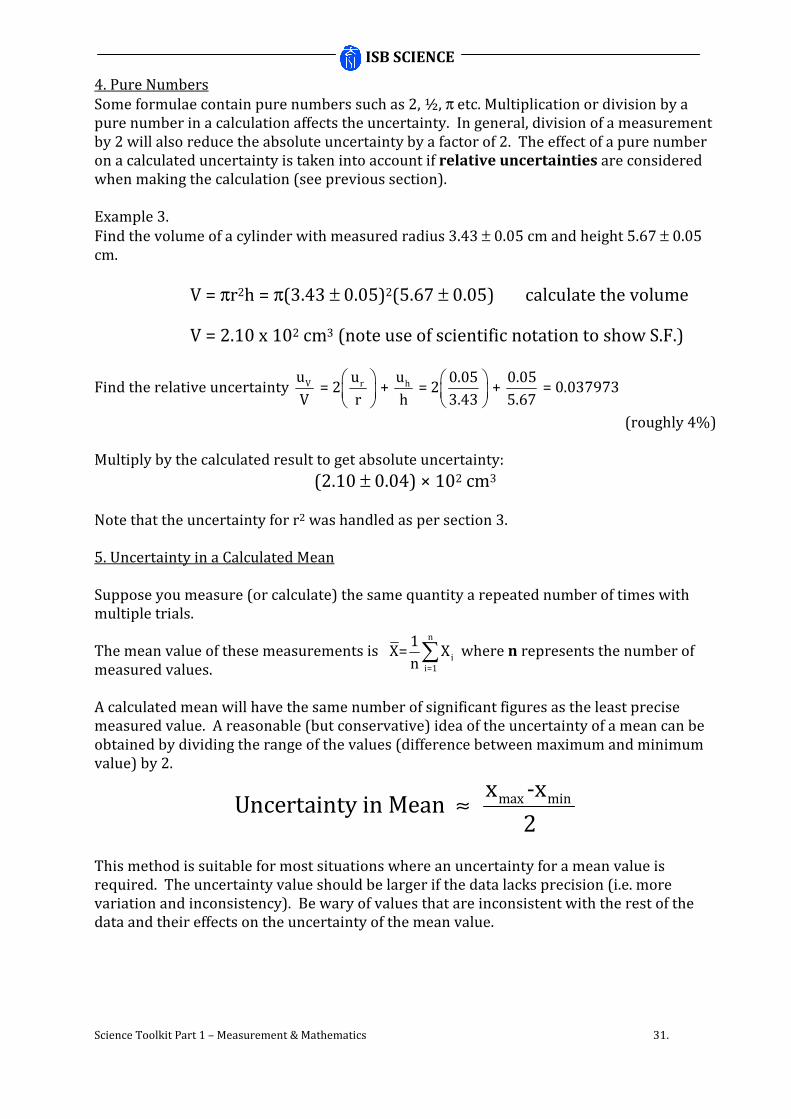
4. Pure Numbers
Some formulae contain pure numbers such as 2, ½, π etc. Multiplication or division by a pure number in a calculation affects the uncertainty. In general, division of a measurement by 2 will also reduce the absolute uncertainty by a factor of 2. The effect of a pure number on a calculated uncertainty is taken into account if relative uncertainties are considered when making the calculation (see previous section). Example 3.
Find the volume of a cylinder with measured radius 3.43 ± 0.05 cm and height 5.67 ± 0.05 cm.
V = πr2h = π(3.43 ± 0.05)2(5.67 ± 0.05) calculate the volume
V = 2.10 x 102 cm3 (note use of scientific notation to show S.F.)
Find the relative uncertainty
V r hu u u 0.05 0.05 = 2 + = 2 + = 0.037973
V r h 3.43 5.67
(roughly 4%) Multiply by the calculated result to get absolute uncertainty:
(2.10 ± 0.04) × 102 cm3 Note that the uncertainty for r2 was handled as per section 3.
5. Uncertainty in a Calculated Mean Suppose you measure (or calculate) the same quantity a repeated number of times with multiple trials. The mean value of these measurements is where n represents the number of measured values.
A calculated mean will have the same number of significant figures as the least precise measured value. A reasonable (but conservative) idea of the uncertainty of a mean can be obtained by dividing the range of the values (difference between maximum and minimum value) by 2.
≈ max minx -xUncertainty in Mean
2
This method is suitable for most situations where an uncertainty for a mean value is required. The uncertainty value should be larger if the data lacks precision (i.e. more variation and inconsistency). Be wary of values that are inconsistent with the rest of the data and their effects on the uncertainty of the mean value.
ISB SCIENCE
Science Toolkit Part 1 – Measurement & Mathematics 32.
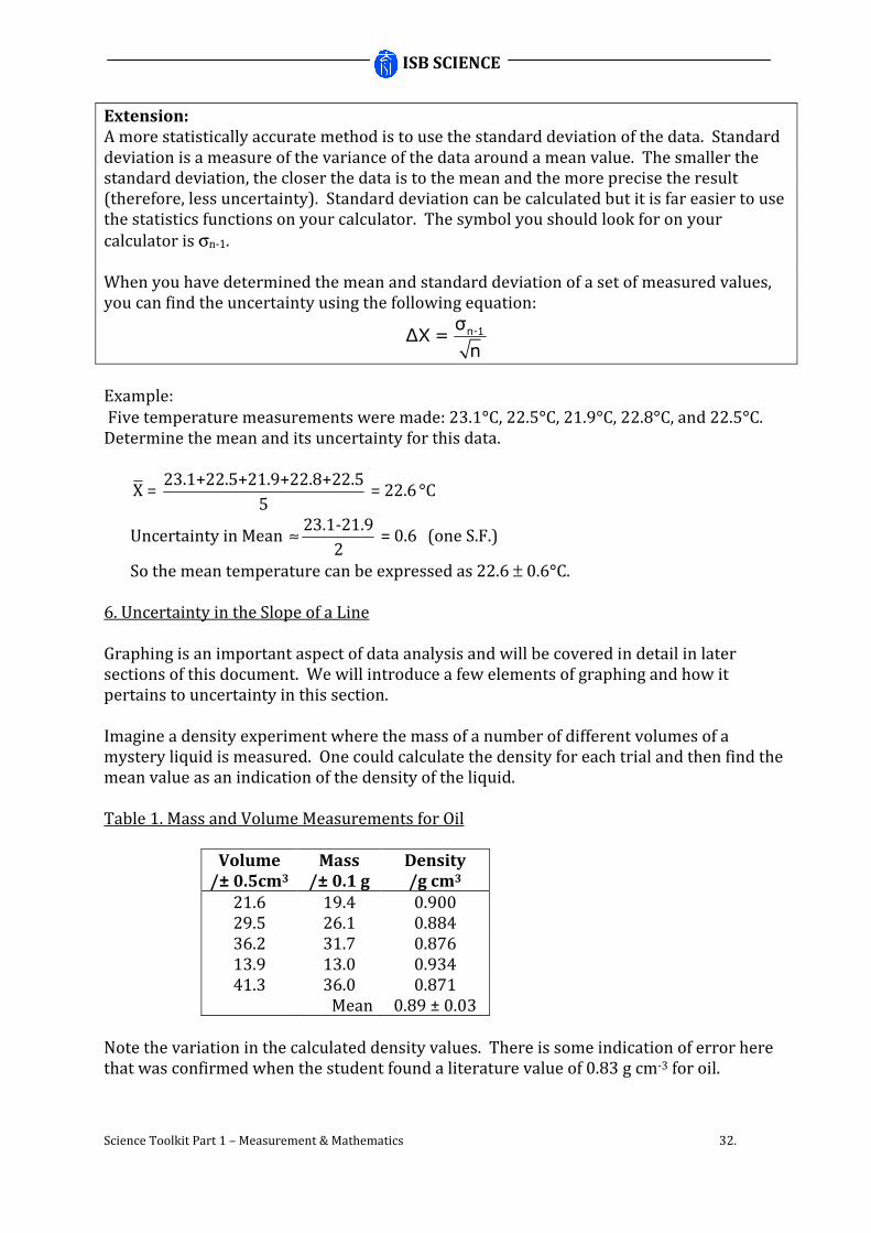
Extension:
A more statistically accurate method is to use the standard deviation of the data. Standard deviation is a measure of the variance of the data around a mean value. The smaller the standard deviation, the closer the data is to the mean and the more precise the result (therefore, less uncertainty). Standard deviation can be calculated but it is far easier to use the statistics functions on your calculator. The symbol you should look for on your
calculator is σn-1. When you have determined the mean and standard deviation of a set of measured values, you can find the uncertainty using the following equation:
n-1σ∆X =
n
Example:
Five temperature measurements were made: 23.1°C, 22.5°C, 21.9°C, 22.8°C, and 22.5°C. Determine the mean and its uncertainty for this data.
23.1+22.5+21.9+22.8+22.5
X = = 22.65
°C
Uncertainty in Mean ≈23.1-21.9
= 0.62
(one S.F.)
So the mean temperature can be expressed as 22.6 ± 0.6°C.
6. Uncertainty in the Slope of a Line Graphing is an important aspect of data analysis and will be covered in detail in later sections of this document. We will introduce a few elements of graphing and how it pertains to uncertainty in this section. Imagine a density experiment where the mass of a number of different volumes of a mystery liquid is measured. One could calculate the density for each trial and then find the mean value as an indication of the density of the liquid. Table 1. Mass and Volume Measurements for Oil
Volume
/± 0.5cm3
Mass
/± 0.1 g
Density
/g cm3
21.6 19.4 0.900 29.5 26.1 0.884 36.2 31.7 0.876 13.9 13.0 0.934 41.3 36.0 0.871
Mean 0.89 ± 0.03
Note the variation in the calculated density values. There is some indication of error here that was confirmed when the student found a literature value of 0.83 g cm-3 for oil.

ISB SCIENCE
Science Toolkit Part 1 – Measurement & Mathematics 33.
A better option would be to plot mass vs volume on a graph and find the slope of the best fit line. The slope of this line is a better indicator of the liquid density for a number of reasons.
• The graph provides a good indication of possible systematic error (you get a y-intercept where you expected the graph to pass through the origin)
• Large random errors are immediately obvious (you would observe a point is way off the best fit line)
y = 0.84x + 1.3
0.0
5.0
10.0
15.0
20.0
25.0
30.0
35.0
40.0
0 10 20 30 40 50
Volume
Mass
The slope and equation of a best fit line immediately provides a mathematical expression for the relationship between two variables. In this case it gives a density value (0.84) much closer to the accepted value and an intercept of 1.3 (indicating a systematic error – such as an improperly zeroed balance, that would produce the variation seen in the calculated values for each trial) As with other calculated values, the slope of a best fit line will also have an
uncertainty associated with it.
You are already aware that the uncertainty in a variable can be shown graphically by using error bars. When determining uncertainty in the slope of a best fit line, you will consider error bars for y-values only. Consider the following graphs maximum best fit line minimum
ISB SCIENCE
Science Toolkit Part 1 – Measurement & Mathematics 34.
Uncertainty bars can be used to draw lines of maximum and minimum slope. Try to draw these lines as representative of the data and symmetrical around the best fit line. When you do this, the value of (maximum slope – best fit slope) should be roughly equal to (best fit slope – minimum). This value is a reasonable expression of the uncertainty of the best fit line slope. For example, if a best fit line slope is calculated to be 4.6, the minimum slope found to be ~
4.4 and the maximum slope is ~ 4.8, then the best fit line slope can be expressed as 4.6 ± 0.2. Just a final note on graphing. MS Excel is a powerful tool and it is recommended that you learn to use it to deal with data, calculations and graphing. It is limited however and students should try to understand these limitations (for example, Excel will not omit an erroneous point on a graph from its best fit line function).
ISB SCIENCE
Science Toolkit Part 1 – Measurement & Mathematics 35.
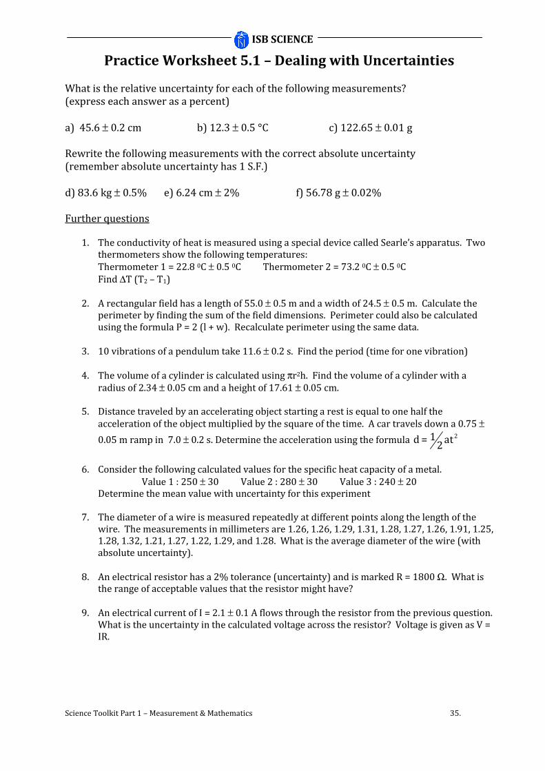
Practice Worksheet 5.1 – Dealing with Uncertainties What is the relative uncertainty for each of the following measurements? (express each answer as a percent)
a) 45.6 ± 0.2 cm b) 12.3 ± 0.5 °C c) 122.65 ± 0.01 g Rewrite the following measurements with the correct absolute uncertainty (remember absolute uncertainty has 1 S.F.)
d) 83.6 kg ± 0.5% e) 6.24 cm ± 2% f) 56.78 g ± 0.02%
Further questions
1. The conductivity of heat is measured using a special device called Searle’s apparatus. Two thermometers show the following temperatures:
Thermometer 1 = 22.8 0C ± 0.5 0C Thermometer 2 = 73.2 0C ± 0.5 0C
Find ∆T (T2 – T1)
2. A rectangular field has a length of 55.0 ± 0.5 m and a width of 24.5 ± 0.5 m. Calculate the perimeter by finding the sum of the field dimensions. Perimeter could also be calculated using the formula P = 2 (l + w). Recalculate perimeter using the same data.
3. 10 vibrations of a pendulum take 11.6 ± 0.2 s. Find the period (time for one vibration)
4. The volume of a cylinder is calculated using πr2h. Find the volume of a cylinder with a
radius of 2.34 ± 0.05 cm and a height of 17.61 ± 0.05 cm.
5. Distance traveled by an accelerating object starting a rest is equal to one half the
acceleration of the object multiplied by the square of the time. A car travels down a 0.75 ±
0.05 m ramp in 7.0 ± 0.2 s. Determine the acceleration using the formula 21d = at
2
6. Consider the following calculated values for the specific heat capacity of a metal.
Value 1 : 250 ± 30 Value 2 : 280 ± 30 Value 3 : 240 ± 20 Determine the mean value with uncertainty for this experiment
7. The diameter of a wire is measured repeatedly at different points along the length of the
wire. The measurements in millimeters are 1.26, 1.26, 1.29, 1.31, 1.28, 1.27, 1.26, 1.91, 1.25, 1.28, 1.32, 1.21, 1.27, 1.22, 1.29, and 1.28. What is the average diameter of the wire (with absolute uncertainty).
8. An electrical resistor has a 2% tolerance (uncertainty) and is marked R = 1800 Ω. What is the range of acceptable values that the resistor might have?
9. An electrical current of I = 2.1 ± 0.1 A flows through the resistor from the previous question. What is the uncertainty in the calculated voltage across the resistor? Voltage is given as V = IR.

ISB SCIENCE
Science Toolkit Part 1 – Measurement & Mathematics 36.
Solutions (possibly with some random errors)
Practice Worksheet 1.1 – Scientific Notation Review
a) 3.68 × 10⁴ b) 3.1 × 10⁻² c) 1.01 × 10²
d) 4.05 × 10⁻⁸ e) 2.601 × 10¹⁰ f) 3.2 × 10⁻⁵
g) 0.000274 h) 679.2 i) 5209000 j) 0.00000000491 k) 3.81 l) 72.9
m) 1.740 × 10⁹ n) 3.00 × 10¹⁰ o) 4.50 × 1047
Practice Worksheet 1.3 – SI Prefixes
a) 1.89 Gm b) 4 mL c) 360 kg d) 4.5 cm e) 12.7 ns f) 0.57 mg g) 2.47 mA h) 4.5 dm or 45 cm i) 1.87 × 10⁹ g
j) 6.3 × 10⁻⁵ m k) 5 × 10⁻² s l) 980 m
m) 0.0045 A n) 9.23 × 10⁻⁶ m o) 654 m
p) 7.8 × 10⁻⁴ g
Practice Worksheet 1.4 – Significant Figures
Part 1 a) 4 b) 3 c) 3 d) 2 e) 2 f) 3 g) 3 h) 6 i) 5 j) 6 k) 1 l) 1 m) 4 n) 3 o) 3 p) 3 Part 2 a) 654.646 m b) 655 m c) 700 m d) 1.00 × 102 cm or 1.00 m
e) 7.0 × 103 cm f) 1.250 × 105 mm or 125.0 m Practice Worksheet 2.3 – Estimating Uncertainty
Note the solutions given are reasonable estimates of uncertainty for the measurements given. Your measurements and uncertainties will be different, that is intentional and intended to promote discussion. The answers given are all in proper form. Even if your answers are different, proper form must be used.
Cylinder 1
15 ± 1 mL
Cylinder 2
85 ± 3 mL
Cylinder 3
168 ± 5 mL
Burette 1
31.83 ± 0.05 mL
Burette 2
31.18 ± 0.05 mL
Cylinder 4
62.8 ± 0.3 mL
Temperature 1
28.5 ± 0.5 oC
Length 1
1.5 ± 0.2 cm
Length 2
1.49 ± 0.05 cm
Voltage 1
3.4 ± 0.3 V
Mass 1
17.42 ± 0.05 g
Length 3
1.4 ± 0.1 cm

ISB SCIENCE
Science Toolkit Part 1 – Measurement & Mathematics 37.
Practice Worksheet 2.5 – Calculations with Significant Figures
a) 8.8 b) 6.5 c) 360.2 d) 10 e) 3.39 (3.4) f) 3.01 g cm-3 g) 14 cm2 h) 119 cm2 Precision and Accuracy
Practice Exercise 3.0
Bob is reasonably accurate but not very precise at all. Bob’s final result was lucky. His experimental skills are inconsistent with random errors. Joe is not that accurate or precise either. Sue is very precise but not accurate. Her experimental technique is consistent but has a built in error. Kate is both precise and accurate. These comparisons are QUALITATIVE rather than QUANTITATIVE. See Practice exercise 3.2a below for more detail. Practice Exercise 3.2
Bob 3.9% error Joe 5.6% error Sue 10.9 % error Kate 0.51% error Using % error values to compare an experimental value to an actual value is much more meaningful than saying “our results are close” Practice Worksheet 4.0 – Math and Calculator Review
a) 149000 b) 5.8 c) 0.71 d) 0.00143 e) 2.277
f) 19.0 0 g) 4.1 h) -2 i) 38400
j) m
VD
= k) P
IV
= l) 2
1
2
Frq
kq=
m)
1
1 1i
o
df d
−
= −
n) 2d
ta
= o) 2
2
4lg
T
π×=

ISB SCIENCE
Science Toolkit Part 1 – Measurement & Mathematics 38.
Practice Worksheet 4.2 – Factor Label Method and Unit Conversion
1. 4560 mL 2. 12.4 km 3. 2140 s 4. 4.39 hr 5. 85000 m
6. 4300 s 7. 120 m 8. 1.3×10⁷ min 9. 0.45 kg 10. 39.6 cm
11. 18 m/s 12. 90. km/h 13. 4.5×10⁷ km/day 14. 5.58 atm 15. 301 m
16. 55.8 kg 17. 24 0C 18. 301 K 19. 8.763 dm3 20. 78 min
QUAIZZORP
1. 8 Quats per second 2. 7700 Q2 3. 4600 $nickers 4. 390 Zugs
Practice Worksheet 5.1 – Dealing with Uncertainties
a) 0.44% b) 4.1% c) 0.0082%
d) 83.6 ± 0.4 kg e) 6.2 ± 0.1 cm f) 56.78 ± 0.01 g
1. (5.0 ± 0.1) × 101 0C [this is 50 ± 1 degrees written correctly]
2. 159 ± 4 m
3. 1.16 ± 0.02 s
4. (3.0 ± 0.1) × 102 cm2
5. 18 ± 2 m
6. 260 ± 10
7. 1.27 ± 0.01 mm
8. Range 1764 Ω to 1836 Ω. Voltage = 3800 ± 300 volts

Senior Science Tool Kit
Measurement & Mathematics
Revision 3 – 2007
Mr. D.J. Young

Table of Contents
Section Title Page
1.0 Orders of Magnitude 1 1.1 Expressing Orders of Magnitude – Scientific Notation 2 1.2 Order of Magnitude Estimates 4 1.3 Powers of 10 and the SI System of Measurement 6 2.0 Measurement Skills 9 2.1 Significant Figures 9 2.2 Measurements and Uncertainty 11 2.3 Estimating Uncertainty 12 2.4 Representing Uncertainty 16 2.5 Calculations with Significant Figures 17 3.0 Precision and Accuracy 19 3.1 Errors in Data 21 3.2 Comparing Values in Science 22 4.0 Mathematical Skills 24 4.1 Dimensional Analysis 26 4.2 Factor Label Method 26 5.0 Dealing with Uncertainties 28 5.1 Error Propagation – Uncertainty in Calculated Results 28
Addition and Subtraction 29 Multiplication and Division 29 Exponents and Square Roots 30 Pure Numbers 31 Uncertainty in a Calculated Mean 31 Uncertainty in the Slope of a Line 32
Appendix Solutions to Worksheets 36

ISB SCIENCE
Science Toolkit Part 1 – Measurement & Mathematics 1.
1.0 Orders of Magnitude Study in science deals with both very large and very small numbers.
The order of magnitude of a number is the power of 10 that is closest to the numerical value of a measurement or quantity.
Order of magnitude is closely related to scientific notation (reviewed in the following section) as a change of one order of magnitude is the same as multiplying or dividing a number by 10. For example 3452 is one order of magnitude larger than 345.2 and two orders of magnitude larger than 34.52. The difference between two quantities in orders of magnitude is basically the difference between the base 10 exponents of the two quantities when written in scientific notation.
For example my mass 8.95×101 kg is roughly 1032 or 32 orders of magnitude larger than
the mass of an electron (9.11×10⁻³¹ kg). That is a big difference! Order of magnitude is important when we consider the range of measurements possible in our physical world i.e.
Object Mass (kg)
Electron 9.11 x 10⁻³¹
Proton 1.67 x 10⁻²⁷
Small coin 1.13 x 10⁻³
Mr. Y. 8.95 x 101
Moon 7.35 x 10²²
Sun 1.99 x 1030
Order of magnitude is useful when approaching problems. Science involves numbers (lots of them) and frequent calculations. When you solve a problem, you can estimate your answer to the nearest power of 10, and compare to the solution you have obtained. If the solution differs by a couple of orders of magnitude you have probably made an error (using the calculator, or perhaps a unit conversion mistake or omission). Careless mistakes!?!?!? Example number 1
Suppose you just calculated the density of vegetable oil from lab data to be 9250 g/mL. How do you know this is wrong? What is the most likely error?
Careless mistakes!?!?!? Example number 2
I just calculated the final velocity for a proton that has been accelerated through an electric field. The calculated velocity is 3.45 x10¹² ms-1. Is this value realistic?

ISB SCIENCE
Science Toolkit Part 1 – Measurement & Mathematics 2.
Careless mistakes!?!?!? Example number 3
Check out this answer to a past exam question:
Clearly 7.7 × 10¹² kg is unreasonable.
1.1 Expressing Orders of Magnitude: Scientific Notation Consider the following definition: “One light year is the distance that light travels (in a vacuum) in one year”. Given that the speed of light in a vacuum is about 300 million meters per second, calculate the length of a light year in meters? (see below for answer)
You will no doubt realize that it is convenient to express your answer in scientific notation (ie. it is a really big number). Frequently in physics, very large and very small numbers are expressed in scientific notation. Scientific notation is used to when expressing numbers to the correct number of significant figures and can also make unit conversions quite easy.
You must be comfortable with scientific notation and recognizing
powers of 10. You must be able to enter these numbers in your
calculator correctly if you are to succeed in science courses.
General form for scientific notation is:
M x 10N
Where 1 < M < 10 and N is an integer
[a light year is 9.46 ×××× 1015 m]

ISB SCIENCE
Science Toolkit Part 1 – Measurement & Mathematics 3.
Practice Worksheet 1.1 – Scientific Notation Review Express the following measurements in scientific notation: a) 36800 g
b) 0.031 J c) 101 V
d) 0.0000000405 s e) 26010000000 cm f) 0.000032 m3
Rewrite the following numbers in standard notation: g) 2.74×10⁻⁴
h) 6.792×10² i) 5.209×10⁶
j) 4.91×10⁻⁹ k) 3.81×100 l) 7.29×101
Estimate answers to the following and then evaluate using your calculator. Express the solutions using correct scientific notation: m) n) Estimate: Estimate: Actual: Actual: o)
Estimate: Actual:
3
12
10781.4
10321.8
××
13
5 3 5
22
5.55 10(3.78 10 ) (4.10 10 )
2.73 10
−−
×× × × ×
×
( )23
16
3
8.45 102.04 10
5.75 10
−−
×× ×
×

ISB SCIENCE
Science Toolkit Part 1 – Measurement & Mathematics 4.
1.2 Order of Magnitude Estimates
Fermi's piano tuner problem and other back of envelope estimates
Enrico Fermi designed the first nuclear reactor to achieve a fission chain reaction. As a professor at the University of Chicago, Fermi would challenge his students to solve problems that seemed impossible due to lack of given information. Fermi wanted his students to develop their abilities to make assumptions and estimations and work out rough solutions on the back of an old envelope rather than making detailed (with calculators in your case) calculations. A typical Fermi problem is to determine the number of piano tuners in Chicago given only the population of the city.
Fermi’s solution:
1. Given Chicago has a population of about 3 million people. 2. Assume that the average family has four members so that the number of families in
Chicago must be about 750,000. 3. Assume one out of five families owns a piano, there will be 150,000 pianos in
Chicago. 4. If the average piano tuner worked 5 days a week tuning 4 pianos each day and had a
two week vacation during the summer…. 5. In one year (50 weeks) he would tune 1,000 pianos. Therefore there must be about
150 piano tuners in Chicago.
This method is not guaranteed correct but it is a valid first estimate that might be off by no more than a factor of 2 or 3 but will definitely not inaccurate by an order of magnitude (we should not expect 15 piano tuners, or 1,500 piano tuners).
Solving Fermi problems develop critical skills that lead to success in science
• Fermi questions provide limited information and require assumptions
• Fermi questions require students to ask and answer further questions
• Fermi questions demand estimations often of common everyday values like the mass of a brick or the length of a soccer field.
• Fermi questions emphasize process rather than product

ISB SCIENCE
Science Toolkit Part 1 – Measurement & Mathematics 5.
Practice Worksheet 1.2 – Fermi Problems Strategies
“everything should be made as simple as possible, but no simpler” Einstein. Don’t make numbers more precise than necessary
• Round to the nearest 0, 5 or 10
• Don’t worry about numbers like π (call it 3 .. or even 2) Guess numbers that you don’t know
• Try to use common sense to make good guesses
• Accurate guesses requires experienced common sense … this comes from education …. pay attention
Make complicated geometry simple
• Assume the cow is a sphere Extrapolate from what you do know
• Use ratios
• Use known similar values (for example you could reasonably assume the density of gasoline is 1 g/mL)
Example Fermi questions for you to try
1. How many jelly beans fill a one litre jar?
2. What is the mass of the entire student body of the school?
3. How many water balloons would it take to fill the school gymnasium?
4. How many tennis balls would cover the area of two tennis courts?
5. How high would a pile of one trillion 1 dollar bills reach?
6. How much gasoline is used by all the cars in China in one year?

ISB SCIENCE
Science Toolkit Part 1 – Measurement & Mathematics 6.
1.3 Powers of 10 and the SI System of Measurement The SI System of Measurement
• SI units (Le Systeme International d’Unites) – or more commonly called the metric system.
• Adopted for scientific research in 1960 worldwide, used as general measurement in most countries (USA and UK excepted)
Fundamental SI Units
• cannot be measured in simpler form
• you must know these basic quantities (and generally you need to convert them to solve problems)
Quantity Fundamental
SI unit SI symbol
Length Meter m
Mass Kilogram kg
Time Second s
Electric Current Ampere A
Absolute Temperature Kelvin K
Amount of Substance Mole mol
• some quantities are based on the measurement of two or more fundamental quantities – units for these are called derived units - a common example would be velocity (ms-1)
• note that the IBO accepted format for the velocity unit is ms-1 and not m/s. This applies to all derived units. (Get used to it!)
• the fundamental SI units are based on standards ex. the standard kilogram is a platinum-iridium cylinder kept in France, a standard second is the time for 9 192 631 770 vibrations of a cesium atom.

ISB SCIENCE
Science Toolkit Part 1 – Measurement & Mathematics 7.
SI Unit Prefixes Previously, the fundamental SI units were discussed. Much like scientific notation, larger and smaller SI units are created by multiplying the value of the base unit by factors of 10 (or 10-1). For example, the SI prefix “kilo” means multiplied by 103. Therefore 1 kilometer equals 103 or 1000 meters.
Common Prefixes used with SI Units
Prefix Symbol Meaning Order of Magnitude
giga- G 1 000 000 000 109
mega- M 1 000 000 106
kilo- k 1 000 103
hecto- h 100 102
deka- da 10 101
base unit 1 100
deci- d 0.1 10-1
centi- c 0.01 10-2
milli- m 0.001 10-3
micro- µ 0.000 001 10-6
nano- n 0.000 000 001 10-9
Not all prefixes are commonly used. More detailed tables can often be found in your textbook or data booklets.
Note that there are many different ways a measurement can be expressed. 125 000 meters could be expressed as:
125 km 0.125 Mm
1.25 × 10⁵ m
ALWAYS PAY ATTENTION TO UNITS! Calculations in science involve the use of formulae and mathematical constants. Formulae often involve variables representing several different measured quantities. It is common practice in science that standard units are implied for the variables in the formulae. For example:
• most distances are measured in meters
• most masses are measured in kilograms or grams
• most time periods are measured in seconds.
Quantities measured in other units must first be converted
before a correct solution can be obtained. Quite often, this can be simply accomplished by applying orders of magnitude. For
example, the quantity 636 µm can be easily converted to meters and entered directly into
the calculator as 636 ×××× 10-6 m.
replaces µ

ISB SCIENCE
Science Toolkit Part 1 – Measurement & Mathematics 8.
Practice Worksheet 1.3 – SI Prefixes
Rewrite the following measurements using appropriate metric prefixes. There could be more than one reasonable answer for some questions. a) 1.89 × 10⁹ m b) 0.004 L
c) 360000 g d) 4.5 × 10⁻² m
e) 1.27 × 10⁻⁸ s f) 0.00057 kg
g) 0.00247 A
h) 0.45 m
Write the following in base units (use scientific notation if appropriate) i) 1.87 Gg j) 63 µm
k) 5 cs l) 0.98 km
m) 4.5 mA n) 9230 nm
o) 0.654 km p) 0.78 mg

ISB SCIENCE
Science Toolkit Part 1 – Measurement & Mathematics 9.
Topic 2.0 Measurement Skills Science is a quantitative subject. This means taking measurements and dealing with numbers.
• All measurements consist of two parts: the magnitude of the measurement (the number) and the unit of the measurement.
• Two types of quantities can be measured: scalar quantities and vector quantities. Scalar quantities can be completely described by magnitude and unit. Scalar quantities include mass, time and temperature. Vector quantities additionally require direction to completely describe a measurement. Examples of vector quantities are force and velocity.
• Measurements are never exact. In other words, measurements always contain a
degree of uncertainty. 2.1 Significant Figures (Digits)
• The precision of lab measurements is indicated by the variation in a number of many repeated measurements. The more variation, the lower the precision of the measurement (this tells us how consistent we are when making measurements).
• Precision is also defined by resolution of the measuring instrument. A more “precise” instrument will provide readings with a more digits after the decimal point.
• Significant figures in a measurement include all the digits that are known for “certain” plus one more “uncertain” digit. The uncertain digit is the estimated digit in a measurement
• More precise instruments mean your measurements will have more significant figures (and smaller uncertainties)
How many significant figures are in a measurement?
In any given measurement, all non-zero digits (1 to 9) are always counted as significant. There are special rules for zeros when counting significant figures.
Rule Examples
Zeros between non-zero digits are significant.
40.5 has 3 S.F. 2001 has 4 S.F.
Zeros following a non-zero digit and after a decimal are significant.
5.230 has 4 S.F. 1.00 has 3 S.F.
Zeros before the first non-zero digit are not significant. A single zero used as a place marker before the decimal is NOT significant.
0.000450 has 3 S.F.
0.5 has 1 S.F.
Zeros at the end of a number that does not have a decimal are not significant. Note: Many textbook problems have easy numbers with trailing zeros (ex. 2000 m). It is generally not the intention of the author that this value be considered as 1 S.F.
100 has 1 S.F. 4010 has 3 S.F.

ISB SCIENCE
Science Toolkit Part 1 – Measurement & Mathematics 10.
Practice Worksheet 2.1 – Significant Figures 1. How many significant figures are there in each measurement? a) 727.2 m b) 601 g c) 46.0 mL d)0.044 g
e) 320 cm f) 0.00401 L g) 1060 s h) 123456 mg
i) 12.500 g j) 340.010 mL k) 0.02 m l) 0.5 kg
m) 1.113 × 10³ kg
n)8.00 × 10⁸ m o) 6.80 °C p)7.67 × 101 °C
2. Write the following measurements to the number of significant figures listed
a. 654.64587 m to 6 SF
b. 654.64587 m to 3 SF
c. 654.64587 m to 1 SF
d. 100 cm to 3 SF
e. 7000 cm to 2 SF
f. 125000 mm to 4 SF

ISB SCIENCE
Science Toolkit Part 1 – Measurement & Mathematics 11.
2.2 Measurements and Uncertainty How long is the pencil?
2 3 4 5 When making measurements, the last digit of the measurement is always an estimate. This digit is called the uncertain digit (because it is an estimate). When taking a measurement:
• read the scale to the smallest graduation (the limit of measurement)
• estimate the next digit of the measurement This produces a more precise measurement but with a degree of uncertainty. When deciding on a reasonable uncertainty in a measurement, one must consider the instrument itself AND how the measurement is made. A general starting point for an uncertainty determination is:
A rule of thumb: The degree of
uncertainty is at a minimum equal to
half of the smallest graduation on the
measurement scale and is often
greater.
Uncertainty and error are two very different concepts. An error in measurement is how far the measured quantity is from the actual value. Errors are not part of measurement uncertainty although discussion of errors is important in lab reporting. The quantity of uncertainty reflects the precision of the measuring tool used (for example a 10 mL graduated cylinder is more precise than a 100 mL cylinder) AND any limitations in the measurement technique itself (for example, using a meter stick to measure the rebound height of a bouncing ball). The National Institute of Standards and Technology (NIST) uses the symbol “u” to represent uncertainty. For a temperature measurement, the uncertainty would be represented as “uT”.
?

ISB SCIENCE
Science Toolkit Part 1 – Measurement & Mathematics 12.
Example
Using a thermometer marked in 1 °C increments, a sample
measurement for T ± uT might be 23.1 ± 0.5 °C.
• 23.1 is the measured quantity (T)
• 1 is the estimated digit
• ± 0.5 is the measurement uncertainty (symbolized by uT
and is one half of the smallest graduation ie. 1 °C)
Key Concept: Notice that the uncertainty ±±±± 0.5
• Has only one non-zero digit (one significant figure)
• The non-zero digit has the same place value as the estimated digit in the measured value.
This type of uncertainty is called an absolute uncertainty because it is measured in the same units as the measured quantity.
Relative (or percent) uncertainty expresses the absolute uncertainty as a proportion (or percentage) of the measured quantity. For the previous measurement of T (temperature).
2.3 Estimating Uncertainty It will not take you much time in the laboratory to realize that determining the uncertainty of a particular measurement is not as simple as the previous example. Although the precision of the measuring instrument affects the uncertainty, it is not the only factor. Quite often, other environmental factors must be considered. Example 1. You are measuring the length of a rubber band being stretched by hanging weights. The weights are oscillating slightly and it is difficult to get the ruler edge to line up directly with the rubber band. Are there other factors (besides the ruler precision) contributing to uncertainty in the length measurement?
0.5relative uncertainty 0.021645 or ~ 2.2%
T 23.1
Tu= = =

ISB SCIENCE
Science Toolkit Part 1 – Measurement & Mathematics 13.
Example 2. You roll a steel ball down a ramp off the desk. It lands on a piece of carbon paper on the floor. You repeat the procedure 10 times (producing 10 dots) and then attempt to measure the horizontal distance the ball travels (on average) from the edge of the desk. The 10 dots are scattered about. How would you make the measurement and estimate the uncertainty?
In all science labs this year, you will never make a measurement without including an
uncertainty. How you choose that uncertainty will depend on what the measurement tool was and how it was used. The uncertainty included will have to be reasonable. This will take practice and judgement. Your estimates of uncertainty may be different than a classmate. It is important that your answer is reasonable and that the place value of the uncertainty is the same as that of the last digit of the measurement. A larger uncertainty reflects less confidence in the value of a measurement.

ISB SCIENCE
Science Toolkit Part 1 – Measurement & Mathematics 14.
Practice Worksheet 2.3 – Estimating Uncertainty Make measurements for each of the situations shown in the diagrams. Include uncertainty with each measurement.
Example 1. Measure the volume in each of the three
pipettes shown.
From left to right:
Pipette 1 : 5.75 ± 0.05 mL
Pipette 2 : 3.0 ± 0.3 mL
Pipette 3 : 0.35 ± 0.05 mL All are acceptable measurements.
Example 2. What is the diameter of this penny?
Answer: Around 1.9 ± 0.2 cm This is not a realistic measurement because in the lab the ruler would be placed across the penny. The diagram does not allow that so the uncertainty is more conservative.
Cylinder 1 Cylinder 2 Cylinder 3

ISB SCIENCE
Science Toolkit Part 1 – Measurement & Mathematics 15.
Burette 1 (initial volume) Burette 2 (final volume)
Temperature 1 Length 1 (scale in cm) Voltage 1
Length 2
Mass 1 Length 3 (scale in cm)

ISB SCIENCE
Science Toolkit Part 1 – Measurement & Mathematics 16.
2.4 Representing uncertainty Tables Uncertainty should be included in the table column headings with units. Example 1
Velocity
/ ± 0.3 ms-1
4.6
5.9
7.4
Example 2 (uncertainties of calculated values may not always be the same)
Velocity / ms-1
4.6 ± 0.2
5.9 ± 0.3
7.4 ± 0.4
Graphs Measurement uncertainty is shown graphically using uncertainty bars.
The data point is a small dot that has been circled. The uncertainty bars show that the point could reasonably be anywhere inside the shaded rectangle. The uncertainty is also noted on the axis label with the unit of measurement. On some graphs, the uncertainty bars may be too small to show relative to the graph scale. When this occurs, a note should be added indicating that this is the case.
The backslash is another form of notating units in a table or on a graph. You can also place units in parentheses
Note that the last digit of each measurement and the uncertainty are in the same place value column

ISB SCIENCE
Science Toolkit Part 1 – Measurement & Mathematics 17.
2.5 Calculations with Significant Figures
Data processing involves the mathematical manipulation of data values recorded in the laboratory. When doing calculations with measurements, significant figures must be considered when writing a final solution. In general, the more significant figures, the more precise a measurement is. A calculation cannot make a result more precise so the final solution can never be more precise than the least precise value used in the calculation. In other words, significant figures tell you how to round off your final answer. For addition and subtraction calculations
i. Determine the place value of the last significant digit in each number added or subtracted.
ii. Identify the measurement with the last digit of the highest place value. iii. Round the final answer to that place value.
Example: Add the following: 120 cm, 34 cm, 4.5 cm and 0.40 cm. Step 1. Identify the last significant digit in each number. These are the digits
underlined in the given numbers. Step 2. Identify the digit with the highest place value. This is the “2” in 120 cm as it
is in the 10’s column. Step 3. Add the numbers to get 158.9 cm. This must be rounded to the 10’s column
so the final answer is 160 cm. For multiplication and division (and combined operation) calculations
i. Determine the number of significant figures of all the measurements used in the calculation.
ii. Identify the measurement with the least number of significant figures. iii. Round the final answer to that number of significant figures.
Example: What is the area of a rectangle measuring 7.5 cm × 2.25 cm? Count significant figures: 7.5 cm has 2 S.F. & 2.25 has 3 S.F. Therefore, the final answer
can only have 2 S.F.
A = L × W
A = 7.5 × 2.25 A = 16.875 A = 17 cm2 (correctly rounded to 2 S.F.)
The IBO’s expectation for complicated calculations is to apply the general rule that the final solution has the same number of significant figures as the least precise measurement.
Extension: To use MS Excel to round appropriately, enter the following formula in the required cell: =ROUND(value,sigfigs-(1+INT(LOG10(ABS(value)))))
The cell containing the number to be rounded is value, and the number of significant figures is sigfigs.

ISB SCIENCE
Science Toolkit Part 1 – Measurement & Mathematics 18.
63.45
7.2
(17.3 9.2)
1.25
(77.67 45.786)
9.87231
6.78 2.3 19.3 35.6 14.5 9.87
9
(6.0 56.6) (12.34 4.09)
14.4 (16.9 3.12)
−
×
+ + + + +
+ ×−
×
-3
Do this . .
mD=
V
m 112.5D = =
l×w×h (11.2×2.34×5.21)
D = 0.824 g cm -3
Try to avoid this . .
V = l×w×h = 11.2×2.34×5.21
V = 136.54368
m 112.5D = =
V (136.54368)
D = 0.824 g cm
Practice Worksheet 2.5 – Calculations with Significant Figures Solve the following problems, show complete solutions when formulae or equations apply. Round your answer to the correct number of significant figures, watch for correct units!
a. b. c. d. e.
f. A rock is found to have a volume of 18.65 cm3 and a mass of 56.2 g. Find the density of the rock.
g. A triangle is measured to have a base of 4.5 cm
and a height of 6.05 cm. What is the area of the triangle?
h. A circle has a diameter of 12.3 cm. What is the
area of the circle?
Important notes:
• When performing calculations that have multiple steps, carry all decimals and round off once at the end of the calculation. DO NOT ROUND each calculation.
• It is good practice to rearrange equations and make substitutions so that one overall calculation can be performed on the calculator rather than a series of steps. For example: to determine the density of a 112.5 g block with the following dimensions; length 11.2 cm, width 2.34 cm and height 5.21 cm.
• Many textbooks and worksheets do not consider significant figures when writing sample problems that use easy numbers like 1500 m. In these types of problems, we will consider the trailing zeros (the ones at the end) to be significant. It would be more correct though to use scientific notation or more appropriate units. For example: to properly write 1500 m to show that the last zeros are significant (total 4 S.F.)
ANSWER: 1.500 × 10³ m OR 1.500 km

ISB SCIENCE
Science Toolkit Part 1 – Measurement & Mathematics 19.
3.0 Precision and Accuracy
• Good science involves measuring a physical quantity a number of times.
• We often use the terms precision and accuracy interchangeably when talking about an experimental result. Technically, they mean very different things. Remember this when writing lab reports.
Accuracy is an indication of how close a measurement is to the accepted value. Precision is an indication of the agreement among a number of measurements made in the same way. Alternatively, precision is often used when referring to the resolution of a measuring instrument. We say that instruments that are scaled with small graduations are more precise than those with larger graduations.

ISB SCIENCE
Science Toolkit Part 1 – Measurement & Mathematics 20.
Practice Worksheet 3.0 – Precision and Accuracy
Consider the following table of results for 4 students who are trying to measure “g”, the acceleration of a falling object due to gravity. The accepted value for “g” is 9.81 ms-2. Table 1: Measurements of ‘g’ in Physics class
Trial Bob Joe Sue Kate
1 7.83 9.53 8.70 9.72
2 11.61 9.38 8.75 9.86
3 8.85 8.87 8.77 9.70
Mean 9.43 9.26 8.74 9.76
Compare the accuracy and precision of each student.
Whose results are meaningful, and whose results are questionable?

ISB SCIENCE
Science Toolkit Part 1 – Measurement & Mathematics 21.
3.1 Errors in Data There are three types of errors that can occur when collecting data: Human Errors
Includes the following
• misreading scales
• mistakes copying raw data to final lab report
• not following procedures properly You should be aware of this and act to avoid such errors. This type of error can be mentioned in a lab report to explain a rogue data point or inconsistency. Human errors however SHOULD NOT be the focus of a formal evaluation of procedure and results. Systematic Error
A systematic error is an error that tends to be consistent for all measurements (built in). Reasons include:
• badly made instruments
• poorly calibrated (zero error)
• instrument parallax (reading a scale at an angle)
• limitations of experiment (e.g. friction or air resistance) Systematic errors can often be minimized or corrected before the investigation is carried out. They should definitely be considered when discussing results. The best indication of a systematic error is a y-intercept value appearing on a data plot for the experiment. For this reason alone, never force a graph through the origin – you may be ignoring a
significant error.
Example: In the previous experiment, it is likely that friction would have an effect on the value of “g” calculated in a falling object experiment.
• How would it affect the result?
• Would you see a different effect depending on the object used in the experiment?

ISB SCIENCE
Science Toolkit Part 1 – Measurement & Mathematics 22.
Random Errors
Random errors result from unpredictable variation in the performance of the instrument/operator or fluctuations in the physical environment. For example, when using a stopwatch to measure the time for a pendulum to complete 10 cycles, it is unlikely that the results for 5 repeated trials will be exactly the same. Why?
• Random errors follow statistical distributions and can be minimized by: collecting enough data (multiple trials) well designed experiments (control of variables, consistency) use the most sensitive (precise) instruments
• On a graph, random errors show as the distribution of points around a best fit line. The more points on the line, the less random error.
• If measurements have a large uncertainty due to limitations in measurement techniques, it is expected that this will contribute to random error.
Variations and inconsistencies due to random error are relatively easy to spot by simply looking at the data. When discussing this type of error, ensure that it is supported by the data and that a realistic improvement for minimizing its effect is mentioned.
3.2 Comparing Values in Science It is very common in science to use lab results to obtain a final value that is compared to an accepted value found in the literature. These comparisons are an indication of the accuracy of the experimental value because they compare an experimental value to the
accepted actual value. The absolute error in an experimental value is determined by:
absolute error = experimental - actual
The relative error is more meaningful and is calculated by:
experimental - actualrelative error =
actual
Relative error is often expressed as a percent and is sometimes referred to as the percent error.
percent error = relative error × 100%

ISB SCIENCE
Science Toolkit Part 1 – Measurement & Mathematics 23.
The percent difference is the difference between two calculated or experimental values. You may use this if you wish to compare two measurements of the same quantity but made in different ways.
1 2
value 1 - value 2percent difference =
v +v
2
Sample problem: An experiment was done to calculate the speed of a wave moving along a string. One method produced a value of 13.4 ms-1 while a second different method produces a value of 12.1 ms-1. Determine the percent difference between these two experimental values.
Practice Worksheet 3.2 – Absolute and Percent Errors Consider the following table of results for 4 students who are trying to measure “g”, the acceleration of a falling object due to gravity. The accepted value for “g” is 9.81 ms-2. Table 1: Measurements of ‘g’ in Physics class
Trial Bob Joe Sue Kate
1 7.83 9.53 8.70 9.72
2 11.61 9.38 8.75 9.86
3 8.85 8.87 8.77 9.70
Mean 9.43 9.26 8.74 9.76
Calculate the absolute and percentage error for each student.

ISB SCIENCE
Science Toolkit Part 1 – Measurement & Mathematics 24.
4.0 Mathematical Skills Applying mathematics is a critical aspect of problem solving in science. Many textbooks provide excellent mathematical review sections in the Appendices. Use these to refresh your knowledge or as a quick reference. The basic math skills required for senior science courses are as follows: Arithmetic and Computation
• Make calculations involving addition, subtraction, multiplication and division.
• Recognize and use expressions in decimal and standard form (scientific notation). Make calculations involving numbers in scientific notation.
• Use calculators to evaluate exponents; reciprocals; roots; logarithms to base 10; logarithms to base e; powers; arithmetic means; degrees; radians; quadratic equations; natural sine, cosine and tangent functions and their inverse.
• Express fractions as percentages and vice versa. Algebra
• Change the subject of an equation by manipulation of the terms including integer and fractional indices and square roots.
• Solve simple algebraic equations, and simultaneous linear equations involving two variables.
• Substitute numerical values into algebraic equations.
• Comprehend the meanings of (and use) the symbols /, <, >, ≤, ≥, ±, ≈, ∆x, ∝, x. Geometry and Trigonometry
• Calculate areas of right-angled and isosceles triangles, circumferences and areas of circles, volumes of rectangular blocks, cylinders and spheres, and surface areas of rectangular blocks, cylinders and spheres. Relevant formulas need not be recalled.
• Use Pythagoras’ theorem, similarity of triangles and recall that the angles of a triangle add up to 1800 (and of a rectangle, 3600).
• Understand the relationship between degrees and radians, and translate from one to the other.
• Recall the small angle approximations (tan θ ≅ sin θ for small angles). It is also extremely important that you are familiar with and know how to use your calculator efficiently and correctly. You do not learn how to solve problems by watching the teacher do them. To be successful, you must attack each problem aggressively and do not be afraid to make mistakes.
BRING A CALCULATOR TO EVERY CLASS AND MAKE SURE YOU USE IT TO OBTAIN
THE CORRECT SOLUTION FOR EVERY EXAMPLE PROBLEM WE DO!

ISB SCIENCE
Science Toolkit Part 1 – Measurement & Mathematics 25.
Practice Worksheet 4.0 – Math and Calculator Review Evaluate the following using your calculator. Express your answer with the proper number of significant digits.
a) (386)2 b) √34
c) cos 45o
d) 1/698
e) 0.7247π f) sin-1 0.325
g)
h) i)
Rewrite the following equations for the variable requested
j) solve for V
k) solve for I l) solve for q1
m) solve for di
n) solve for t o) solve for g
12
2
1084
2345637
×
××
.823
8367
001.
.
.=
x
556
337242
.
)( ×−
V
mD =
2
2
1atd =
0
111
ddf i
+=
2
21
r
qqkF =IVP ×=
g
lT π2=

ISB SCIENCE
Science Toolkit Part 1 – Measurement & Mathematics 26.
4.1 Dimensional Analysis The dimension of a measurement refers to its unit. Dimensional analysis means exactly that pay attention to units! This simple example shows the benefit of dimensional analysis. We know that speed is measured in m/s (or ms-1) and that speed is a rate (a measurement of how a quantity changes with time). If a formula for speed was given as:
tv =
d
You might notice something wrong right away just by considering the units involved. Dividing time by distance will not yield the desired unit m/s but rather would produce a quantity with the unit s/m. The formula is therefore incorrect.
4.2 Factor Label Method Factor label method is a technique utilizing dimensional analysis to ensure the math is correct. A conversion factor is an equality statement between two units. For example 1 m = 100 cm and 1 hour = 60 min are both conversion factors (Tip: check out the website for a useful unit conversion program). Factor-label method involves multiplying the value to be converted by appropriate conversion factors written as fractions (which have a value of 1). When arranging conversion factors as fractions, the numerator and denominator are determined by what unit is desired in the final answer and by what unit needs to be cancelled. Example 1: Convert 4.5 m to cm.
Step 1. Determine the required conversion factor: 1 m = 100 cm Step 2. Multiply 4.5 m by the conversion factor written as fraction.
100 cm4.5 m×
1 m “m” cancels leaving “cm” and the answer 450 cm
You may need to multiply by a series of factors to get the conversion you want. Example 2: Convert 1.25 days to seconds
24 hours 60 min 60 s1.25 days × × × = 108000 s
1 day 1 hour 1 min
In this example, days are converted to hours, then hours to minutes, and finally minutes to seconds to get the answer.
Significant figure rules do not apply to unit conversion factors

ISB SCIENCE
Science Toolkit Part 1 – Measurement & Mathematics 27.
Dimensional analysis is a very useful technique that can be applied to help ensure the correct method is used for solving all kinds of problems. Example 3: How many grams of water can be made by the combustion of 4.6 g of
hydrogen gas with excess oxygen according to the equation 2 H2 + O2 2 H2O?
-12 22-1
2
4.6 g H 2 H O × ×18.0 g mol = 41 g H O
2 H2.0 g mol
Practice Worksheet 4.2 – Unit Conversion You may need to look up some unit conversion factors to complete these unit conversion problems:
1. Convert 4.56 L to mL 2. Convert 12400 m to km 3. Convert 35.6 min to seconds 4. Convert 15800 s to hours 5. Convert 85 km to meters 6. Convert 1.2 hours to seconds
7. Convert 1.2×105 mm to meters
8. Convert 8.9×10³ days to minutes 9. Convert 450 g to kilograms 10. Convert 15.6 inches to centimeters 11. Convert 65 kmh-1 to ms-1 12. Convert 25 ms-1 to kmh-1
13. Convert the speed of light (3.0×10⁸ ms-1) to km day-1
14. Convert 565 kPa to atmospheres (atm)
15. Convert 987 ft to meters 16. Convert 123 lbs to kilograms 17. Convert 76 0F to Celsius 18. Convert 28 0C to Kelvin 19. Convert 8763 mL to dm3 20. Convert 1.3 hours to minutes
IN A FAR AWAY GALAXY ON THE PLANET QUAIZZORP
One Nard (Nd) is 8 Quats (Q) long, therefore 1 Nd = 8 Q. A mushy can run 60 Nards in one minute (60 Nd min-1). Answer the following questions in the space provided. Don’t forget units.
1. How many Quats per second can a mushy run?
2. Fred owns a mushy pasture measuring 10.0 Nards by 12 Nards (or 120 Nd2). How many square Quats (Q2) does Fred own?
3. All mushys weigh exactly 12 Zugs. Fred sells 80.2 % of his 150 mushys at a rate of
3.2 $nickers per Zug. How many $nickers did Fred get?
4. Fred’s mushy mashing machine can manage to mash 6.0 mushys in 11 minutes. How many Zugs of mashed mushy can it produce in 1.0 hours?

ISB SCIENCE
Science Toolkit Part 1 – Measurement & Mathematics 28.
5.0 Dealing with Uncertainties Recall, when making measurements:
• every measurement has an uncertainty associated with it
• by convention, the minimum uncertainty usually equals half the limit of the smallest graduation on the scale of the measurement instrument
• the uncertainty is always written with ONE significant digit
• the place setting of the uncertainty matches the place setting of the estimated digit in the measurement
5.1 Error Propagation – Uncertainty in Calculated Results It is quite common to measure two or more quantities (each with their individual uncertainties) and combine the information to calculate a desired value. For example, to find density we may measure mass and volume and then calculate the density using the appropriate equation. The uncertainty in the original mass and volume measurements will propagate to the calculated density value. Consider mass to be 11.4 ± 0.2 g and the volume to be 9.6 ± 0.5 cm3.
Possible maximum density = 11.6 ÷ 9.1 = 1.2747 g cm-3
Actual calculated density value = 11.4 ÷ 9.6 = 1.1875 g cm-3
Possible minimum density = 11.2 ÷ 10.1 = 1.1089 g cm-3
As the calculated result can only have 2 S.F., it would be expressed as 1.2 ± 0.1 g cm-3.
The range of the calculated result is 1.1 to 1.3 g cm-3 and encompasses both the
maximum and minimum possible values.
There are more efficient ways of determining the propagated uncertainty in a calculated result. The method used depends on the type of calculations conducted.
+ 0.0872
- 0.0786

ISB SCIENCE
Science Toolkit Part 1 – Measurement & Mathematics 29.
(X×Y)R=
Z
Addition and Subtraction of Measured Quantities
When adding or subtracting measurements – ADD THE UNCERTAINTIES
Let’s say you make 3 measurements: X ± uX, Y ± uY, and Z ± uZ where uX, uY, and uZ are the absolute uncertainties of the respective measurements. You are required to combine these measurements to obtain the result R using the following formula:
R = X + Y – Z
The absolute uncertainty in R is determined by
uR ≈≈≈≈ uX + uY + uZ
Note the rule for addition or subtraction is the same. ADD the uncertainties. Example 1.
Find the perimeter of a rectangle measuring 5.0 ± 0.5 m by 3.0 ± 0.5 m.
P = (5.0 ± 0.5 m) + (3.0 ± 0.5 m) + (5.0 ± 0.5 m) + (3.0 ± 0.5 m)
P = 16.0 ± 2.0 m
P = 16 ± 2 m (uncertainty must be rounded to one significant figure) We again could look at it in terms of maximum and minimum values for the measurements i.e. maximums 5.5 m and 3.5 m, minimums 4.5 m and 2.5 m. If all the maximum measurements were used in the calculations, the perimeter would be 18 m. If all the minimum values were used, the perimeter would be 14 m. Note that these results match the error range of the original calculated result. 2. Multiplication and Division of Measured Quantities Uncertainties can also be expressed as a proportion of the measured value (RECALL relative uncertainty). When completing multiplication, or division calculations, ADD
THE RELATIVE UNCERTAINTIES. So if the relative uncertainty in R is determined by
≈
R X Y Zu u u u+ +
R X Y Z

ISB SCIENCE
Science Toolkit Part 1 – Measurement & Mathematics 30.
To find the absolute uncertainty in the result R, multiply the relative uncertainty by
the calculated value for R
≈
RR
uu R•
R
Example 2.
Find the density of a liquid sample with a measured mass of 40.5 ± 0.5 g and a volume of
93.0 ± 0.5 mL. Density is calculated by dividing mass by volume.
-1
D
m 40.5±0.5D= = =0.435 g mL ±u
V 93.0±0.5
To find uD , first find the relative uncertainty
VD m uu u 0.5 0.5 = + = + = 0.017722
D m V 40.5 93.0
(about 2%) To find the absolute uncertainty
≈DD
uu = D • =0.435 × 0.017722 = 0.0077091 0.008
D
(remember one significant figure)
The final answer would be a density of 0.435 ±±±± 0.008 g/mL
3. Exponents and Square Roots Exponents are essentially multiplication operations ie. x2 is “x” multiplied by itself. If a value is squared in a formula, its relative uncertainty would be added to itself according to the rule outlined in Section 2. The relative uncertainty would therefore be:
x x xu u u + = 2
x x x
Similarly x3 would have a relative uncertainty of 3 times the relative uncertainty of x.
Square roots are treated similarly. Recall 1/2x = x , so if a square root is involved in the calculation, the relative uncertainty is multiplied by ½ when it is considered. You will not encounter this situation very often.

ISB SCIENCE
Science Toolkit Part 1 – Measurement & Mathematics 31.
∑n
ii=1
1X= X
n
4. Pure Numbers
Some formulae contain pure numbers such as 2, ½, π etc. Multiplication or division by a pure number in a calculation affects the uncertainty. In general, division of a measurement by 2 will also reduce the absolute uncertainty by a factor of 2. The effect of a pure number on a calculated uncertainty is taken into account if relative uncertainties are considered when making the calculation (see previous section). Example 3.
Find the volume of a cylinder with measured radius 3.43 ± 0.05 cm and height 5.67 ± 0.05 cm.
V = πr2h = π(3.43 ± 0.05)2(5.67 ± 0.05) calculate the volume
V = 2.10 x 102 cm3 (note use of scientific notation to show S.F.)
Find the relative uncertainty
V r hu u u 0.05 0.05 = 2 + = 2 + = 0.037973
V r h 3.43 5.67
(roughly 4%) Multiply by the calculated result to get absolute uncertainty:
(2.10 ± 0.04) × 102 cm3 Note that the uncertainty for r2 was handled as per section 3.
5. Uncertainty in a Calculated Mean Suppose you measure (or calculate) the same quantity a repeated number of times with multiple trials. The mean value of these measurements is where n represents the number of measured values.
A calculated mean will have the same number of significant figures as the least precise measured value. A reasonable (but conservative) idea of the uncertainty of a mean can be obtained by dividing the range of the values (difference between maximum and minimum value) by 2.
≈ max minx -xUncertainty in Mean
2
This method is suitable for most situations where an uncertainty for a mean value is required. The uncertainty value should be larger if the data lacks precision (i.e. more variation and inconsistency). Be wary of values that are inconsistent with the rest of the data and their effects on the uncertainty of the mean value.

ISB SCIENCE
Science Toolkit Part 1 – Measurement & Mathematics 32.
Extension:
A more statistically accurate method is to use the standard deviation of the data. Standard deviation is a measure of the variance of the data around a mean value. The smaller the standard deviation, the closer the data is to the mean and the more precise the result (therefore, less uncertainty). Standard deviation can be calculated but it is far easier to use the statistics functions on your calculator. The symbol you should look for on your
calculator is σn-1. When you have determined the mean and standard deviation of a set of measured values, you can find the uncertainty using the following equation:
n-1σ∆X =
n
Example:
Five temperature measurements were made: 23.1°C, 22.5°C, 21.9°C, 22.8°C, and 22.5°C. Determine the mean and its uncertainty for this data.
23.1+22.5+21.9+22.8+22.5
X = = 22.65
°C
Uncertainty in Mean ≈23.1-21.9
= 0.62
(one S.F.)
So the mean temperature can be expressed as 22.6 ± 0.6°C.
6. Uncertainty in the Slope of a Line Graphing is an important aspect of data analysis and will be covered in detail in later sections of this document. We will introduce a few elements of graphing and how it pertains to uncertainty in this section. Imagine a density experiment where the mass of a number of different volumes of a mystery liquid is measured. One could calculate the density for each trial and then find the mean value as an indication of the density of the liquid. Table 1. Mass and Volume Measurements for Oil
Volume
/± 0.5cm3
Mass
/± 0.1 g
Density
/g cm3
21.6 19.4 0.900 29.5 26.1 0.884 36.2 31.7 0.876 13.9 13.0 0.934 41.3 36.0 0.871
Mean 0.89 ± 0.03
Note the variation in the calculated density values. There is some indication of error here that was confirmed when the student found a literature value of 0.83 g cm-3 for oil.

ISB SCIENCE
Science Toolkit Part 1 – Measurement & Mathematics 33.
A better option would be to plot mass vs volume on a graph and find the slope of the best fit line. The slope of this line is a better indicator of the liquid density for a number of reasons.
• The graph provides a good indication of possible systematic error (you get a y-intercept where you expected the graph to pass through the origin)
• Large random errors are immediately obvious (you would observe a point is way off the best fit line)
y = 0.84x + 1.3
0.0
5.0
10.0
15.0
20.0
25.0
30.0
35.0
40.0
0 10 20 30 40 50
Volume
Mass
The slope and equation of a best fit line immediately provides a mathematical expression for the relationship between two variables. In this case it gives a density value (0.84) much closer to the accepted value and an intercept of 1.3 (indicating a systematic error – such as an improperly zeroed balance, that would produce the variation seen in the calculated values for each trial) As with other calculated values, the slope of a best fit line will also have an
uncertainty associated with it.
You are already aware that the uncertainty in a variable can be shown graphically by using error bars. When determining uncertainty in the slope of a best fit line, you will consider error bars for y-values only. Consider the following graphs maximum best fit line minimum

ISB SCIENCE
Science Toolkit Part 1 – Measurement & Mathematics 34.
Uncertainty bars can be used to draw lines of maximum and minimum slope. Try to draw these lines as representative of the data and symmetrical around the best fit line. When you do this, the value of (maximum slope – best fit slope) should be roughly equal to (best fit slope – minimum). This value is a reasonable expression of the uncertainty of the best fit line slope. For example, if a best fit line slope is calculated to be 4.6, the minimum slope found to be ~
4.4 and the maximum slope is ~ 4.8, then the best fit line slope can be expressed as 4.6 ± 0.2. Just a final note on graphing. MS Excel is a powerful tool and it is recommended that you learn to use it to deal with data, calculations and graphing. It is limited however and students should try to understand these limitations (for example, Excel will not omit an erroneous point on a graph from its best fit line function).

ISB SCIENCE
Science Toolkit Part 1 – Measurement & Mathematics 35.
Practice Worksheet 5.1 – Dealing with Uncertainties What is the relative uncertainty for each of the following measurements? (express each answer as a percent)
a) 45.6 ± 0.2 cm b) 12.3 ± 0.5 °C c) 122.65 ± 0.01 g Rewrite the following measurements with the correct absolute uncertainty (remember absolute uncertainty has 1 S.F.)
d) 83.6 kg ± 0.5% e) 6.24 cm ± 2% f) 56.78 g ± 0.02%
Further questions
1. The conductivity of heat is measured using a special device called Searle’s apparatus. Two thermometers show the following temperatures:
Thermometer 1 = 22.8 0C ± 0.5 0C Thermometer 2 = 73.2 0C ± 0.5 0C
Find ∆T (T2 – T1)
2. A rectangular field has a length of 55.0 ± 0.5 m and a width of 24.5 ± 0.5 m. Calculate the perimeter by finding the sum of the field dimensions. Perimeter could also be calculated using the formula P = 2 (l + w). Recalculate perimeter using the same data.
3. 10 vibrations of a pendulum take 11.6 ± 0.2 s. Find the period (time for one vibration)
4. The volume of a cylinder is calculated using πr2h. Find the volume of a cylinder with a
radius of 2.34 ± 0.05 cm and a height of 17.61 ± 0.05 cm.
5. Distance traveled by an accelerating object starting a rest is equal to one half the
acceleration of the object multiplied by the square of the time. A car travels down a 0.75 ±
0.05 m ramp in 7.0 ± 0.2 s. Determine the acceleration using the formula 21d = at
2
6. Consider the following calculated values for the specific heat capacity of a metal.
Value 1 : 250 ± 30 Value 2 : 280 ± 30 Value 3 : 240 ± 20 Determine the mean value with uncertainty for this experiment
7. The diameter of a wire is measured repeatedly at different points along the length of the
wire. The measurements in millimeters are 1.26, 1.26, 1.29, 1.31, 1.28, 1.27, 1.26, 1.91, 1.25, 1.28, 1.32, 1.21, 1.27, 1.22, 1.29, and 1.28. What is the average diameter of the wire (with absolute uncertainty).
8. An electrical resistor has a 2% tolerance (uncertainty) and is marked R = 1800 Ω. What is the range of acceptable values that the resistor might have?
9. An electrical current of I = 2.1 ± 0.1 A flows through the resistor from the previous question. What is the uncertainty in the calculated voltage across the resistor? Voltage is given as V = IR.
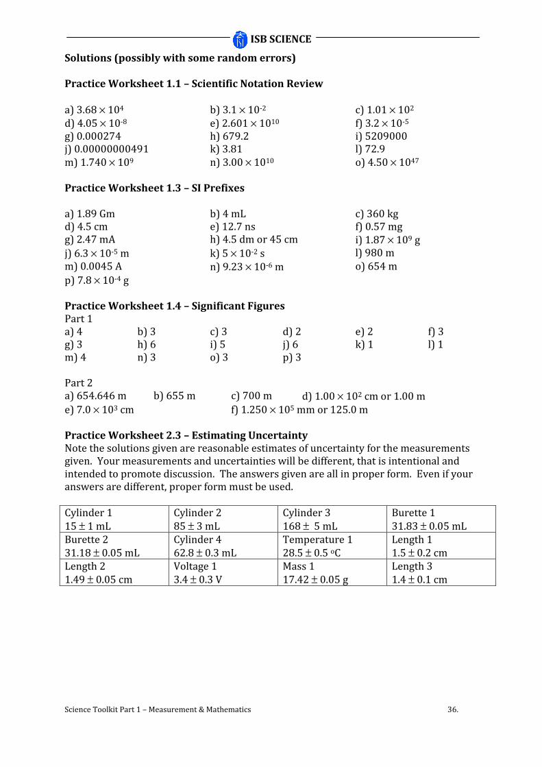
ISB SCIENCE
Science Toolkit Part 1 – Measurement & Mathematics 36.
Solutions (possibly with some random errors)
Practice Worksheet 1.1 – Scientific Notation Review
a) 3.68 × 10⁴ b) 3.1 × 10⁻² c) 1.01 × 10²
d) 4.05 × 10⁻⁸ e) 2.601 × 10¹⁰ f) 3.2 × 10⁻⁵
g) 0.000274 h) 679.2 i) 5209000 j) 0.00000000491 k) 3.81 l) 72.9
m) 1.740 × 10⁹ n) 3.00 × 10¹⁰ o) 4.50 × 1047
Practice Worksheet 1.3 – SI Prefixes
a) 1.89 Gm b) 4 mL c) 360 kg d) 4.5 cm e) 12.7 ns f) 0.57 mg g) 2.47 mA h) 4.5 dm or 45 cm i) 1.87 × 10⁹ g
j) 6.3 × 10⁻⁵ m k) 5 × 10⁻² s l) 980 m
m) 0.0045 A n) 9.23 × 10⁻⁶ m o) 654 m
p) 7.8 × 10⁻⁴ g
Practice Worksheet 1.4 – Significant Figures
Part 1 a) 4 b) 3 c) 3 d) 2 e) 2 f) 3 g) 3 h) 6 i) 5 j) 6 k) 1 l) 1 m) 4 n) 3 o) 3 p) 3 Part 2 a) 654.646 m b) 655 m c) 700 m d) 1.00 × 102 cm or 1.00 m
e) 7.0 × 103 cm f) 1.250 × 105 mm or 125.0 m Practice Worksheet 2.3 – Estimating Uncertainty
Note the solutions given are reasonable estimates of uncertainty for the measurements given. Your measurements and uncertainties will be different, that is intentional and intended to promote discussion. The answers given are all in proper form. Even if your answers are different, proper form must be used.
Cylinder 1
15 ± 1 mL
Cylinder 2
85 ± 3 mL
Cylinder 3
168 ± 5 mL
Burette 1
31.83 ± 0.05 mL
Burette 2
31.18 ± 0.05 mL
Cylinder 4
62.8 ± 0.3 mL
Temperature 1
28.5 ± 0.5 oC
Length 1
1.5 ± 0.2 cm
Length 2
1.49 ± 0.05 cm
Voltage 1
3.4 ± 0.3 V
Mass 1
17.42 ± 0.05 g
Length 3
1.4 ± 0.1 cm

ISB SCIENCE
Science Toolkit Part 1 – Measurement & Mathematics 37.
Practice Worksheet 2.5 – Calculations with Significant Figures
a) 8.8 b) 6.5 c) 360.2 d) 10 e) 3.39 (3.4) f) 3.01 g cm-3 g) 14 cm2 h) 119 cm2 Precision and Accuracy
Practice Exercise 3.0
Bob is reasonably accurate but not very precise at all. Bob’s final result was lucky. His experimental skills are inconsistent with random errors. Joe is not that accurate or precise either. Sue is very precise but not accurate. Her experimental technique is consistent but has a built in error. Kate is both precise and accurate. These comparisons are QUALITATIVE rather than QUANTITATIVE. See Practice exercise 3.2a below for more detail. Practice Exercise 3.2
Bob 3.9% error Joe 5.6% error Sue 10.9 % error Kate 0.51% error Using % error values to compare an experimental value to an actual value is much more meaningful than saying “our results are close” Practice Worksheet 4.0 – Math and Calculator Review
a) 149000 b) 5.8 c) 0.71 d) 0.00143 e) 2.277
f) 19.0 0 g) 4.1 h) -2 i) 38400
j) m
VD
= k) P
IV
= l) 2
1
2
Frq
kq=
m)
1
1 1i
o
df d
−
= −
n) 2d
ta
= o) 2
2
4lg
T
π×=

ISB SCIENCE
Science Toolkit Part 1 – Measurement & Mathematics 38.
Practice Worksheet 4.2 – Factor Label Method and Unit Conversion
1. 4560 mL 2. 12.4 km 3. 2140 s 4. 4.39 hr 5. 85000 m
6. 4300 s 7. 120 m 8. 1.3×10⁷ min 9. 0.45 kg 10. 39.6 cm
11. 18 m/s 12. 90. km/h 13. 4.5×10⁷ km/day 14. 5.58 atm 15. 301 m
16. 55.8 kg 17. 24 0C 18. 301 K 19. 8.763 dm3 20. 78 min
QUAIZZORP
1. 8 Quats per second 2. 7700 Q2 3. 4600 $nickers 4. 390 Zugs
Practice Worksheet 5.1 – Dealing with Uncertainties
a) 0.44% b) 4.1% c) 0.0082%
d) 83.6 ± 0.4 kg e) 6.2 ± 0.1 cm f) 56.78 ± 0.01 g
1. (5.0 ± 0.1) × 101 0C [this is 50 ± 1 degrees written correctly]
2. 159 ± 4 m
3. 1.16 ± 0.02 s
4. (3.0 ± 0.1) × 102 cm2
5. 18 ± 2 m
6. 260 ± 10
7. 1.27 ± 0.01 mm
8. Range 1764 Ω to 1836 Ω. Voltage = 3800 ± 300 volts