ANALYSIS OF GAS SAMPLES FROM COALBED METHANE WELLS IN SULLIVAN COUNTY, INDIANA USING GAS CHROMATOGRAPHY

Senior Thesis

Submitted in partial fulfillment of the requirements for the Bachelor of Science Degree

At The Ohio State University

By

Chad Niddery

The Ohio State University

December 2016

Approved By

Thomas H. Darrah, Advisor

School of Earth Sciences

Table of Contents

Abstract ……………………………………………………………….1

Acknowledgements…………..………………………………………..2

Introduction…………………………………………………………....3

Goals and Objectives…………………………………………………..6

Methods…………………………………………………......................8

Results………………………………………………………………...13

Discussion……………………………………………………………..14

Conclusion………………………………………………………….....18

Recommendations for future work…………………………………....19

Figures ………………………………………………………………..20

Tables…….…………………………………………….......................27

References Cited……………………………………………………...32

1

Abstract

Although there has been an increase in natural gas production from coalbed methane

(CBM) reservoirs in the past few decades, there are multiple inadequately known aspects of

CBM reserves. To understand the systematics of CBM production, twenty gas samples were

collected from producing coalbed methane wells in Sullivan County, Indiana. These wells are

producing from the Springfield and Seelyville coal seam units in the Illinois Basin and have been

characterized for their noble gas chemistry previously. Here, the hydrocarbon molecular

composition, isotopic composition of carbon and hydrogen in methane, and major gas

composition (N2, CO2) are reported. One of the goals of this experiment is to use the composition

of produced gases to determine the relative proportions of major inert gases compared to

economically viable hydrocarbon gases. Another goal of this thesis is to use the composition of

the produced gases to determine if natural gas formation in coal seams in the Illinois Basin is

formed by biogenic processes or thermogenic processes. Based on the analyses conducted in this

experiment, it appears that the wells have a dry gas composition (<1% ethane plus) and contain

2.7 to 10.6% non-hydrocarbon gases (N2, CO2). Based on the presence of ethane in the majority

of wells, one can conclude that there is a mixture of biogenic and thermogenic natural gas

forming in the Springfield and Seelyville coal seams.

Key Words: coalbed methane, Illinois Basin, hydrocarbon molecular composition, isotopic

composition of methane

2

Acknowledgements

I would like to thank Dr. Thomas Darrah for supporting this project, allowing me to be

part of this ongoing research project, and his guidance throughout the research process. I would

also like to acknowledge Myles Moore, M.S. for his assistance in sample collection, analysis,

GC training, research, and writing of this project. I wish to express my sincere thanks to my

entire family back in Canada for their unceasing encouragement and support throughout this

journey. I would like to take this opportunity to record my sincere thanks to all the faculty

members in the School of Earth Sciences and all the valuable guidance they have given me. Each

one of you has taught me more than I could have imagined, from minerals buried miles

underground to simple life lessons, every minute has been gold to me. I would like to reach out

and especially thank Dr. Carey, Dr. Barton, Dr. Krissek, Dr. Darrah, Dr. Lyons, and Dr. Grottoli.

Every day I walked the halls and each of you took two minutes out of your busy schedules to ask

how my day, hockey, life, or school was going, and I am extremely grateful and indebted to each

and every one of you for always supporting me, always having patience with me, and always

encouraging me to stick with what I love the most. Lastly, my sense of gratitude goes out to one

and all who, directly, or indirectly, have lent their helping hand in this venture!

3

Introduction

The ever-growing need to reduce carbon emissions has driven scientific and industry

research away from coal toward the extraction of lower polluting, unconventional energy

resources such as coalbed methane (CBM) and other sources of natural gas (Kerr, 2010; Darrah

et al. 2014). The relatively recent dependence on unconventional resources has produced many

questions about the genetic source (biogenic vs. thermogenic), migration (in situ versus trapped),

and evolution (e.g., degradation by microbes or other oxidizing reactions) of these natural gas

deposits (Burruss and Laughrey, 2010; Tilley and Muehlenbachs, 2012; Hunt et al., 2012; Darrah

et al., 2014; Darrah and Poreda, 2012). To address these issues, I examined the molecular and

isotopic composition of natural gas samples from the Illinois Basin. The samples used in this

study were acquired from Sullivan County, Indiana because it is an ideal location for coalbed

methane (CBM) production (Figures 1 and 2).

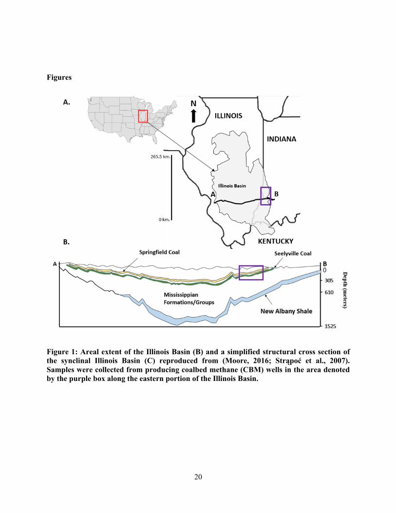
This study area is in close vicinity to the first economically viable CBM project in the

Illinois Basin and sits between multiple active CBM/New Albany Shale projects. The coal fields

accessed for CBM production in this area are near the center of the largest surface coal mine east

of the Mississippi River and is also just east of the highest gas content coal measured in the

Illinois Basin (Buschbach and Kolata, 1990).

The Illinois Basin is an oval-shaped syncline spanning about 1.55 x104 square kilometers

and extending from central Illinois to western Indiana and northwestern Kentucky (Buschbach

and Kolata, 1990). It is bounded by the Mississippi River Arch to the northwest, the Kankakee

Arch to the northeast, the Ozark dome to the southwest, and the New Madrid Rift Complex to

the south (Buschbach and Kolata, 1990). The structural and hydrographic features separate the

4

Illinois Basin from adjacent basins such as the Appalachian Basin (to the east), the Forest City

Basin (to the west), and the Michigan Basin (to the northeast) (Buschbach and Kolata, 1990).

The Illinois Basin is an intracratonic basin that that formed during Appalachian tectonics

spanning from approximately 530 to 280 million years ago (Strąpoć et al., 2007). Sedimentation

in the Illinois Basin occurred during transgressive phases and led to infills up to 3.7 x103 meters

thick near the basin center, which largely consisted of shallow to deep marine sediments (Strąpoć

et al., 2007). During the Devonian, sedimentation occurred within a semi-restricted basin that

produced a stratified, anoxic, marine environment that led to the burial of organic-rich sediments

(Cluff, 1980), which eventually lead to the formation of the New Albany Shale. The New Albany

Shale is the dominant oil- and gas-producing unit in the Illinois Basin (Strapoc et al., 2010).

Currently, depths to the New Albany Shale range from surface outcrop at the edges of the Illinois

Basin to near 1.5 x103 meters at the basin center. Thermal maturities of the New Albany Shale

range from approximately 0.54% vitrinite reflectance (Ro) on the margins of the basin to 1.5%

(Ro) near the center of the basin (Cluff, 1980; Strapoc et al., 2010).

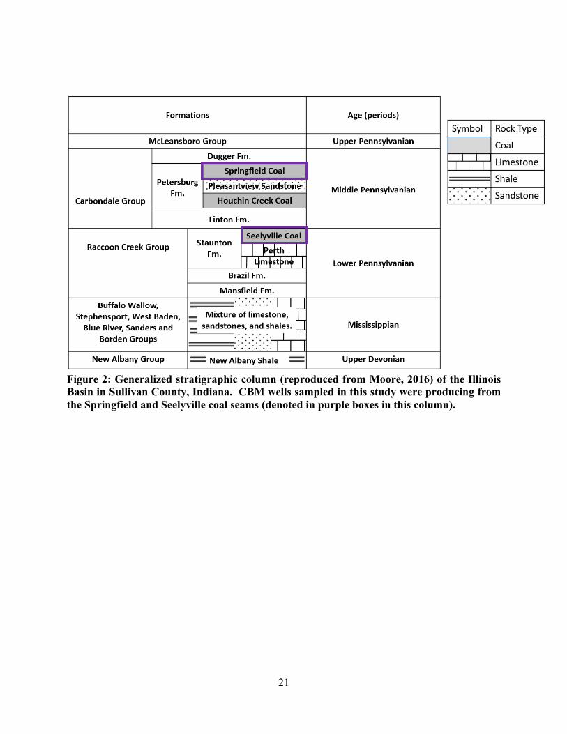
The Pennsylvanian-aged coal-bearing strata in the Illinois Basin were deposited from

~318 to 299 million years ago and are divided into three major units: the McLeansboro, the

Carbondale, and the Raccoon Creek Groups (Strąpoć et al., 2007). Deformation of the Illinios

Basin that formed the macroscopic syncline characterizing the Illinois Basin produced stress on

the coal bed seams, inducing fractures, layer parallel shortening, low amplitude folding, and

cleating. This deformation allowed cleats to expand in size, which allowed natural gas to be

5

released and fresh water to flow in, especially following periods of glaciation (Cluff,

1980; Schlegel et al., 2011; Strapoc et al., 2010).

Gas samples included in this study were collected from producing coal bed methane

wells that are sourced from the Springfield coal seam of the Petersburg Formation and the

Seelyville coal seam of the Linton Formation (purple boxes Figures 1 and 2, Table 1). The

Springfield coal seam ranges in thicknesses of 1.37–1.83 meters and outcrops at the surface and

can get as deep as 260m. The Seelyville ranges in thicknesses of 0.3-3 meters and ranges in

depths from surface to 277 m. deep at the depocenter (Drobniak et al., 2004).

6

Goals and Objectives

Natural gas consists of a mixture of different gases including hydrocarbon gases (CH4,

C2H6, C3H8, C4H10, etc.), major gases (N2, CO2, O2, etc.), noble gases (He, Ne, Ar, etc.) and

sulfides (H2S, COS, etc.) (Akansu et al., 2004; Darrah et al., 2015; Darrah and Poreda, 2012;

Moore, 2012). Determination of gas quality or composition demands that one examines the types

of gases inherently present in each producing well, or reservoirs more broadly. There are

productive gases and inert gases. Productive hydrocarbon gases (methane, ethane, propane, etc.)

are those that add economic value, typically determined by heat content (i.e., BTU or British

Thermal Unit) content, and inert gases (CO2, N2) which do not combust and thus take away value

(Akansu et al., 2004; Moore, 2012).

The overall goals of this research were to analyze the gas samples acquired from producing

coalbed methane wells in Sullivan County, Indiana, to determine the hydrocarbon and non-

hydrocarbon molecular content and the isotopic composition of carbon and hydrogen in methane.

Previous work by our laboratory group has characterized the noble gas composition (Moore,

2016). To be more specific, the following research was conducted to:

1. Evaluate the quality of natural gas produced from unconventional coal seams in Sullivan

County, Illinois (more specifically the Seelyville and Springfield coal seams) to determine its

viability for future coalbed methane production. To do this, one must determine how much of the

producing natural gas is made up of economically viable hydrocarbon gases (e.g., methane,

ethane, propane, butane, pentane), compared to how much is made up of inert (noble gases) and

non-hydrocarbon gases (e.g., N2, CO2) that can reduce profit and or lead to contamination (e.g.,

H2S is toxic, can be fatal, and is also very corrosive to casing and pipelines) (Moore, 2012).

7

2. Identify whether the coalbed methane gas sources are characterized as “dry” or “wet” gas. Dry

natural gas is made up of a much greater proportion of methane compared to other gases. This

study uses 95% as the cut-off between a “dry” gas and wet gas (<95% methane). This study will

quantify how many of the wells in Sullivan County, Indiana are producing dry natural gas vs.

wet natural gas based on methane content. I also compared the hydrocarbon molecular content

(C1/C2+) to see how methane compares with higher-ordered aliphatic hydrocarbon chains in

wells that produce dry vs. wet natural gas.

3. To determine if natural gas being produced from the Springfield and Seelyville coal seams is

biogenic, thermogenic, or a mixture of biogenic and thermogenic origins. Methanogens can

consume organic matter adhered to coals and produce biogenic methane by the reduction of CO2

or acetate fermentation (Ritter et al., 2015; Schoell, 1988). In contrast, thermogenic methane

forms from the thermocatalytic decomposition of kerogen with increasing pressures,

temperatures and burial depths (Tilley and Muehlenbachs, 2006). Based on the stratigraphy, the

Springfield and Seelyville coal seams could be acting as stratigraphic traps for deeper migrated

thermogenic gases. The two processes to form biogenic and thermogenic natural gas could be

taking place in tandem to form a mixture of biogenic and thermogenic natural gas (McIntosh et

al., 2002; Schlegel et al., 2011). One can compare the hydrocarbon molecular content (C1/C2+)

against the isotopic composition of carbon in methane (δ13C-CH4) (Bernard et al., 1978; Whiticar

et al., 1985) and the isotopic composition of hydrogen in methane (δ 2H-CH4) against δ 13C-CH4

(Schoell, 1980; Schoell, 1988) to determine if the natural gases in the Springfield and Seelyville

coal seams are biogenic, thermogenic, or a mixture of biogenic and thermogenic gases.

8

Methods

Sample Selection and Collection:

I measured 20 gas samples collected from actively producing CBM wells for

hydrocarbon geochemistry (molecular; C1/C2+ and stable isotopic composition of carbon and

hydrogen in methane (i.e., δ13C-CH4 and δ 2H-CH4) and major gas composition (N2, CO2) in

Sullivan County, Indiana. Five wells were producing from the Springfield coal seam from CBM

wells at screened intervals of 76 to 210 meters depth (Tables 1; 2; and 3). The data from these

wells are denoted as red diamonds in Figures 5–8. Nine wells were producing from the Seelyville

coal seam from CBM wells at screened intervals of 150 to 210 meters below land surface (Tables

1; 2; and 3). The data from these wells are denoted as red circles in Figures 5–8. Six wells were

sampled that are screened in the Springfield and Seelyville coal seams, these are denoted as

“comingled production” (Tables 1 and 3) and data from these gases are shown by a red triangle

in Figures 5–8.

Gas samples were collected from actively producing CBM wells using 0.95 cm. diameter

and 40.6 cm. long refrigeration-grade copper tubes. Copper tubes were connected in-line of the

CBM well and after flowing production gas for approximately fifteen minutes (>50 copper tube

volumes) through the copper tubes, gas samples were sealed within the copper tube using brass

clamps.

Sample Preparation and Analysis:

In the laboratory, the gas samples in the copper tubes were prepared for analysis by re-

clamping approximately 2.5 cm splits of the copper tubing using stainless steel clamps. Next, the

copper tube was attached to an ultra-high vacuum steel line (total pressure= 1-3 x10-9 torr),

9

which is monitored continuously using a four digit (accurate to the nearest thousandths) 0–20

torr MKS capacitance monometer, using a 0.95 cm. Swagelok ferruled connection. After the

sample connection had been sufficiently evacuated and pressure was verified, an aliquot of the

gas sample was introduced into the ultra-high vacuum line by re-rounding the copper for major

gas composition measurements using a SRS-RGA quadrupole mass spectrometer and SRI Model

8610C SRI GC. This process was repeated sequentially on vacuum introduction lines for the gas

chromatograph for each of the 20 samples.

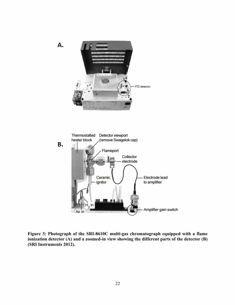
Hydrocarbon and non-hydrocarbon gases were analyzed using an SRI Model 8610C

Multiple Gas Chromatograph #3. The Multiple Gas #3 is a type of Gas Chromatograph that

separates chemical substances and is designed to measure many gases, such as CO, CO2, CH4,

C2H6, C3H8, C4H10, and C5H12 in a single analysis of a sample. After injection of a gas sample,

the instrument generates a series of responses measured in millivolts (mV) on the x-axis against

time on the y-axis. That series of peaks (the visual in the graph for the responses) is known as a

chromatogram. Each peak in the chromatogram represents a specific compound that is present

and the concentration of that compound in the gas sample is determined by comparison to known

standards. The separation of each compound is determined by two limits on the chromatogram;

retention time, which is the time from the point of injection to the peak maximum, and peak area,

which represents the amount of sample present.

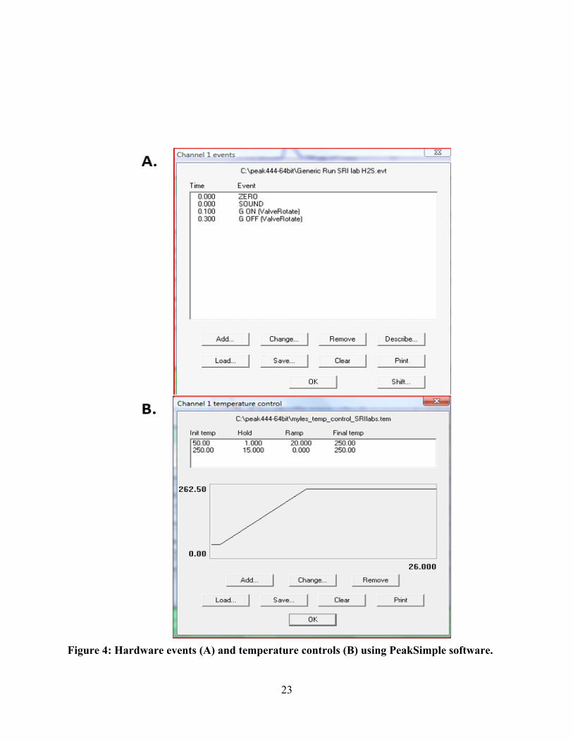
The Multiple Gas #3 GC uses a software program called “PeakSimple” to organize

hardware events and temperature control to test for different compounds using the GC (the

hardware and temperature controls for this study are displayed in Figures 4A and 4B). The

events table is set-up prior to the gas sample being analyzed, it is time-based and the user can

10

decide when to open and close each valve to release the gas sample into the detector (Figure 4A).

As one can see the “G valve” in the hardware event only needs 0.2 seconds for enough sample to

enter to the column and then later on the detector for the analysis to be complete (Moore, 2016).

The temperature control software is also time-based, the user can input at what rate the gas

sample is heated up and for how long the GC will remain heating the gas sample at that

temperature (Figure 4B). It should be noted in this study that the GC held a temperature of

250oC for 15 minutes to ensure that even heavier hydrocarbons like pentane, iso-pentane, and

hexane could be measured. Peaks representing different compounds on a chromatogram typically

will display themselves in increasing molecular weight with increasing time (with iso-butane

peak appearing slightly earlier than butane, iso-pentane peak appearing slightly earlier than

pentane and so forth for hexane). For example, when heating up a sample that contained C1–C6

(shorthand for methane to hexane) hydrocarbons, the first peak would be methane because it is

the lightest gas and would volatize/separate first from the sample, the following peak would be

carbon dioxide because it is the next lightest gas, and would volatize/separate second from the

gas sample.

The SRI Model 8610C Multiple Gas Chromatograph #3 uses helium as its carrier gas and

is equipped with three detectors. Each detector within the GC is used to detect different gases.

The Flame Photometric Detector (FPD) is used to measure sulfur bearing compounds, such as

H2S or SO2. The Thermal Conductivity Detector (TCD) measures the difference in thermal

conductivity in the carrier gas and the sample gas. It is less sensitive than the other detectors,

however it can show all molecules with boiling points below hexane, including; CO2, Methane,

Oxygen, CO, Hydrogen, Nitrogen, Water, and most importantly Hydrocarbons. The TCD will

11

measure all non-sulfur molecules and has a detection range of approximately 0.1% to 100%

(100-1,000,000ppm) (Moore and Whyte, 2015).

Though this GC is equipped with three detectors the detector used in this study is the

Flame Ionization Detector (FID) Methanizer. Hydrogen gas flows through the GC to ensure that

the flame can remain lit. This detector can show a response to any carbon-bearing compound.

The detector does not register a peak for sulfur-containing compounds nor nitrogen and oxygen.

With a detection range from 0.1ppm to almost 100% (Moore and Whyte, 2015) this is the most

sensitive detector for hydrocarbons and therefore this detector is used to determine the

hydrocarbon molecular content (C1/C2+) (Moore and Whyte, 2015).

Methods to analyze gas samples on the MultiGas #3 GC:

Gas samples are stored in an air-tight copper tubing. Tubing is inserted onto vacuum line to syringe 10–20 mL of sample into plastic syringe.

Syringe is cleared with room air in between samples, as is the vacuum line that was used to collect sample.

Inject 10–20mL of sample into GC inlet. *Note-1ml of sample is actually analyzed (the rest clears the line)

Gas flows through channels 1 and 2 detectors. A Haysep-D column (1.83 meters in length) will then separate out the heavier gases, such as; ethane- hexane, CO2, but not O2 and N2, which will show a big peak. Gas will flow through the T.C.D, peaks are not as large as F.I.D, but will be registered earlier on the graph. T.C.D can detect O2, H2, N2, and all molecules with weights less than hexane. Gas flows through F.I.D and peaks will register later but larger because the F.I.D is more sensitive, and the F.I.D will recognize hydrocarbons that weigh less than hexane. Chromatogram will form in the Peaksimple software. The user must identify which peaks are which compounds and the area of the peak to determine what concentration of gas sample is present.

The integration tool in Peaksimple software may have to be used to make sure the software system is identifying peaks correctly and registering the correct areas for the correct compounds.

12

Notes to remember:

1) When a buzz noise is present, and there is a spike on the chromatograph valve G + A on/off because the Gaussian peaks are molecules and the quiet spikes are valves that are changing.

2) T.C.D. Protect: The light turns on when there is no carrier gas present.

For all major and hydrocarbon gas concentrations, the standard analytical errors were all

less than ±3.36% for concentrations above detection limits. Average external position for

hydrocarbon and major gases were determined by “known-unknown” standard experimentation

using an atmospheric air standard (Columbus, Ohio air) and synthetic standards obtained from

the company Praxair. The errors of this analysis are as follows: CH4 (2.19%), C2H6 (2.78%), N2

(1.25%), CO2 (1.06%), H2 (3.41%), and O2 (1.39%) based on daily replicate measurements.

The values for δ13C-CH4 and δ2H-CH4 were measured at Isotech Laboratories

(Champaign, Illinois). The procedures for isotopic analysis of carbon and hydrogen in methane

at Isotech were summarized previously (Darrah et al., 2015; Darrah et al., 2014; Jackson et al.,

2013; Osborn et al., 2011). The isotopic signatures of hydrogen in methane are denoted in per

mil versus Vienna standard means ocean water (VSMOW) with an approximate standard

deviation of ± 0.5 ‰ (Gonfiantini et al., 1995). The isotopic signatures of carbon in methane are

expressed in per mil versus Vienna Peedee belemnite (VDPD), with a standard deviation of ± 0.2

‰ (Gonfiantini et al., 1995). Using chromatographic separation followed by combustion and

dual-inlet isotope ratio mass spectrometry, the detection limits for δ13C-CH4 and δ2H-CH4 were

0.001 and 0.001 (Isotech laboratories, 2012). The methods used in this laboratory followed

previously used methods (Darrah et al., 2013; Darrah et al., 2014; Darrah et al., 2015).

13

Results

Data were collected in this study from 20 CBM wells producing from the Springfield coal

seam, the Seelyville coal seam, and from co-mingled production from both coal seams. For the

interpretation of these results, I treat all 20 samples as one group and recognize that this limits

the interpretations that can be made from this study.

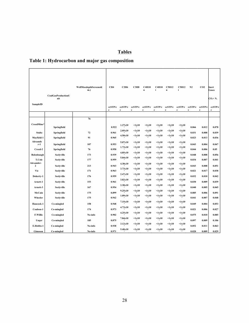
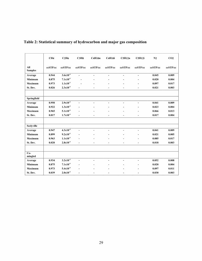
CH4 concentrations ranged from 0.875 to 0.973 ccSTP/cc with 0.944 ccSTP/cc on

average. C2H6 concentrations ranged from 7.1 x 10-5 to 1.1 x 10-3 ccSTP/cc with 3.6 x 10-4

ccSTP/cc on average (Tables 1 and 2). The N2 concentrations ranged from 0.020 to 0.097

ccSTP/cc with 0.045 ccSTP/cc on average. The CO2 concentrations ranged from 0.004 to 0.017

ccSTP/cc with 0.009 ccSTP/cc on average (Tables 1 and 2). The concentrations of C3H8, C4H10n,

C4H10i, C5H12n, C5H12n, and C5H12i (where i denotes iso, meaning C4H10i is isobutane and the n

denotes normal, meaning C4H10n would be butane) were all below the detection limit of 1 x 10-5

ccSTP/cc (Tables 1 and 2).

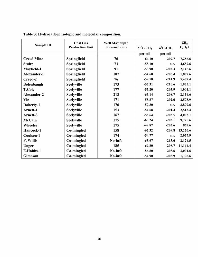
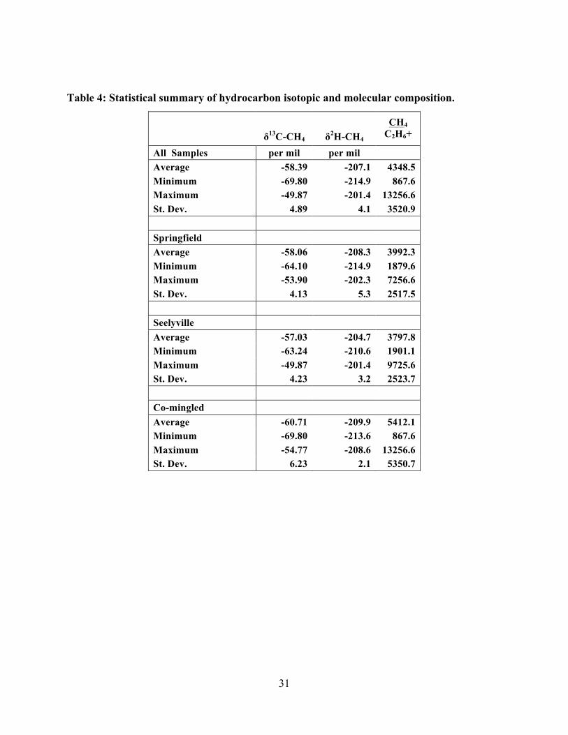
The δ13C-CH4 values ranged from -69.80‰ to -49.87‰ with -58.39 ‰ on average. The

δ2H-CH4 ranged from -214.9‰ to -201.4‰ with an average of -207.1‰. The CH4/C2H6+

(denoted as C1/C2+ in the plots) ratios ranged from 867.6 to 13256.6 with 4348.5 on average

(Tables 3 and 4).

14

Discussion

The overall goals of this research were to: 1) evaluate the quality of natural gas produced

from unconventional coal seams in Sullivan County, Illinois; 2) identify whether the coalbed

methane gas sources are characterized as “dry” or “wet” gas; and 3) to determine if natural gas

being produced from the Springfield and Seelyville coal seams are biogenic, thermogenic, or a

mixture of biogenic and thermogenic origins.

Goal 1: Quality of the Natural Gas

Because the summed concentrations of N2, CO2, He, and Ar account for >99.95% of all non-

hydrocarbon gases, we use these components as metric for the quality of natural gas. With these

parameters, the proportion of non-hydrocarbon gases within the CBM produced gases from this

study area range from 2.7% to 10.6% (Table 1). The samples suggest a range in BTU content

from 817.1 to 923.1 BTU for bulk gas. While it is cost prohibitive to remove N2, He, Ar or other

inert gases, CO2 can be easily removed by cryogenic cycling (USEIA, 2014). Thus, we also

report the BTU content after CO2 removal. After CO2 removal, the BTU values increase by 8.6%

on average and range from 907.1 to 926.3.

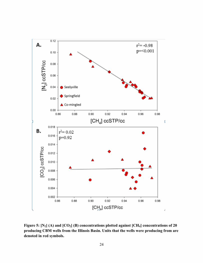
The main factor that seems to control the proportion of hydrocarbon and non-hydrocarbon

gases is the relative proportion of natural gas and water-derived gases in the sample. When

methane concentrations increase, there is a strong negative correlation (r2= -0.98) of decreasing

air-saturated water components, shown by relative to [N2] (Figure 5A). This results from the fact

that methane and N2 (sourced from nitrogen dissolved in groundwater) are the two dominant

gases in all producing natural gas wells. In general, a similar result relative to methane is

observed for argon (Ar).

15

This same observation does not hold true when comparing [CH4] with [CO2] or He

(shown as CO2 in Figure 5B). The lack of correlations between CH4 and either CO2 or He can

likely be attributed to variable roles of microbial activity on CO2, including methanogenic

consumption of CO2 to generate methane and methanotrophic oxidation of organic matter and

natural gas to CO2 (Darrah et al., 2015). In addition, carbon dioxide is highly soluble in water,

and thus can be affected by variable gas-water ratios. Consistent with CO2, He appears to be

more variable and can result from a collection of thermogenic contributions, variations in

groundwater age, and relatively high microbial consumption of natural gas to CO2. As I will

discuss later, the preponderance of data suggests that elevated helium levels are dominated by

the introduction of thermogenic methane.

Goal 2: Dry or Wet Natural Gas

In addition to non-hydrocarbon gases, the composition of hydrocarbons is essential to

evaluating the quality of natural gas samples. While dry gas (dominantly methane) is

exceptionally clean burning and highly energy efficient, wet gas has a higher BTU content, is

more easily transported as a liquid, and as such is more valuable for most commercial operations

(Whiticar et al., 1985). As a result, wet gas is commonly a target for economic hydrocarbon

recovery. For these reasons, wetness (defined as C2+/C1 x 100%) is critical to evaluating the

economic potential of unconventional gas fields.

The range of C1/C2+ from 867.6 to 13,256.6 suggests that all samples collected as part of

this study would be classified as dry gas because the proportion of C2+/C1 x100% (in the

hydrocarbon gas phase only) is significantly less than 5% for all samples (Table 1). While all of

these samples do contain quantifiable ethane levels (but almost no detectable propane or higher

16

order compounds) and significantly lower C1/C2+ than anticipated for a purely microbial end-

member (discussed further below), these gases are all dry gas. Thus, although this field would

represent a clean emitting, and potentially renewable fuel choice, it has relatively low BTU

content compared to other unconventional natural gas fields such as the Marcellus and Utica

(Darrah et al., 2014; Darrah et al., 2015; Burruss and Laughrey, 2010).

Goal 3: Biogenic, Thermogenic or Both?

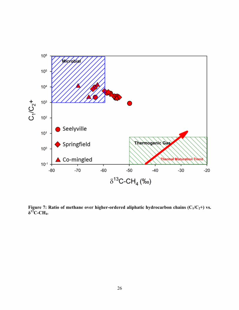
The classic method to distinguish biogenic and thermogenic natural gases compares plots

of C1/C2+ vs. δ13C-CH4 (referred to as “Bernard Plots”; Figure 7) (Bernard et al., 1978; Claypool

et al., 1980; Rice and Claypool, 1981) or plots of δ2H-CH4 vs. δ13C-CH4 (referred to as “Schoell

Plots” or “Whiticar Plots”; Figure 8) (Schoell, 1980; Schoell, 1988; Whiticar et al., 1985). In

these plots, natural gases that have a biogenic origin show highly elevated ratios of C1/C2+

>>~2000 and δ13C-CH4 <~-60 to 65‰, whereas thermogenic gases will have ratios of C1/C2+ =

0.25 to 60 and δ13C-CH4 >~-50‰ (typically >-45‰) (shown in Figures 7 and 8). Since

methanogens cannot produce ethane (Jackson et al., 2013), increasing ethane concentrations can

be indicative of thermogenic contributions to the Springfield and Seelyville coal seams.

When comparing the C1/C2+ against the δ13C-CH4, the majority of samples would be

classified as either “microbial” or near microbial along a mixing trend toward the “thermogenic

gas” composition (Figure 7). The presence of small amount of ethane can be indicative of a

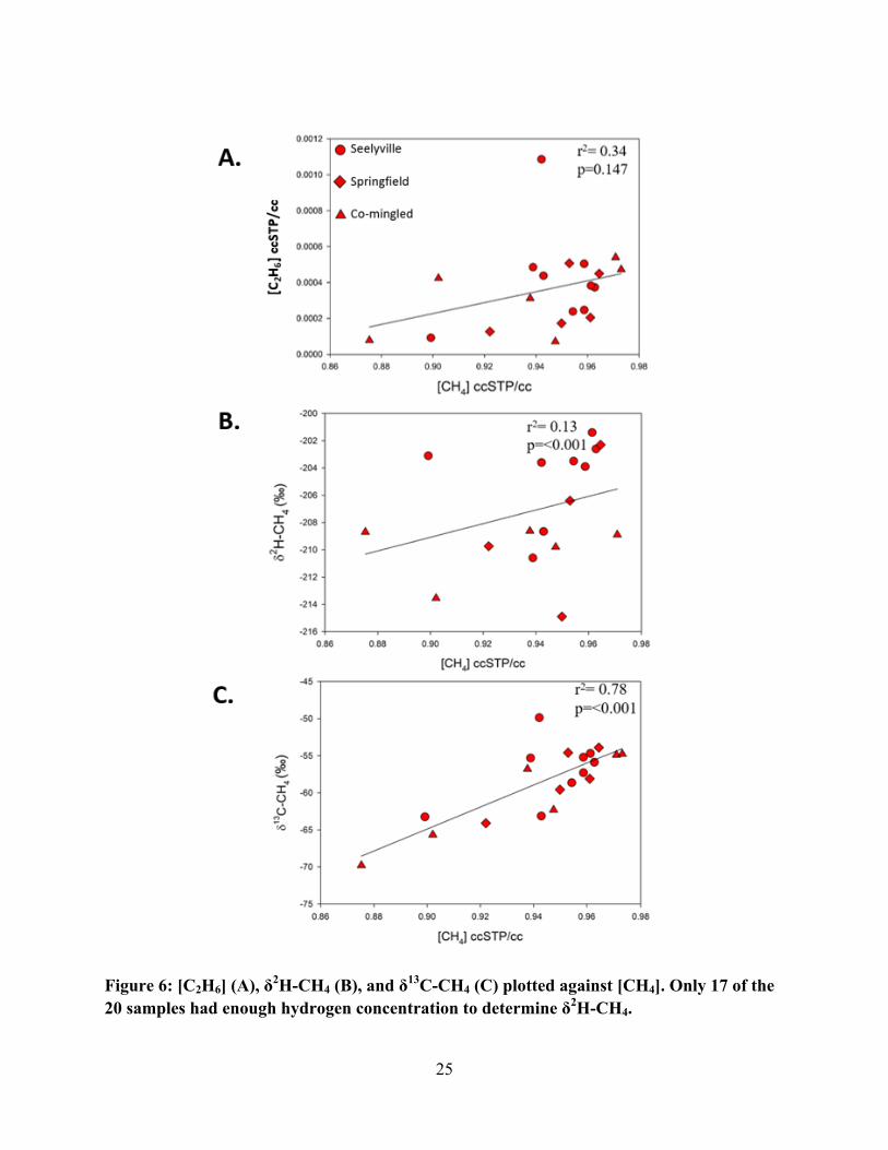
relatively small proportion of thermogenic gas mixing with dominantly biogenic gases. This is

seen in Figure 6A, where there is a weak association of ethane concentrations increasing with

increasing methane concentrations (elevated methane can be thought of as higher proportion of

natural gas with respect to groundwater contributions). As stated earlier, thermogenic natural

gases tend to form more isotopically heavy (more enriched in heavier isotopes) carbon and

17

hydrogen signatures in methane. It seems that more thermogenic in origin natural gases could be

contributing to the Springfield and Seelyville coal seams, because we see relationship between

heavier carbon in methane isotopes with higher methane concentrations (figure 6C).

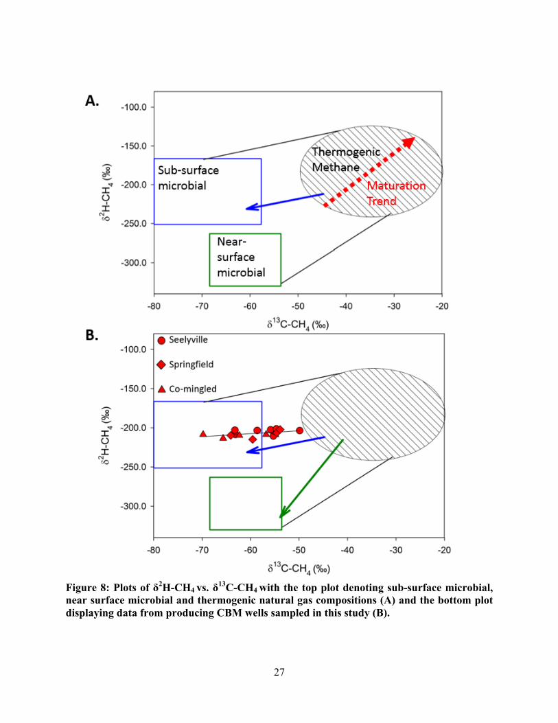
Schoell has demonstrated that δ2H-CH4 can be used to differentiate between near-surface

microbial methane (lighter δ2H-CH4 -350‰ to -270‰) that is associated with acetate

fermentation from sub-surface microbial methane (heavier δ2H-CH4 -250‰ to -170‰) that is

associated with carbon dioxide reduction (Figure 8) (Schoell, 1980). When comparing δ2H-CH4

against δ13C-CH4 of gas samples from producing CBM wells in Sullivan County, Indiana one

can notice that some samples fall in the “sub-surface microbial” zone, but a majority fall along a

mixing line between sub-surface microbial gases and the “thermogenic methane” zone (Figure

8). As stated in the literature review, sub-surface microbes will be using CO2 reduction to form

methane. Therefore, based on Figure 8, it appears that a mixture exists of biogenic natural gas

being formed from CO2 reduction and deeper thermogenic natural gas migrating into the

Springfield and Seelyville coals seams in tandem. Based on the available data, we conclude that

the majority of gases produced from CBM reservoirs in this area is dry gas. These gases likely

result from the combination of biogenic and thermogenic end-members, possibly in shallow

water-dominated coal seams.

18

Conclusions

During this study, I collected 20 gas samples from CBM wells producing from the

Springfield and Seelyville coal seams in Sullivan County, Indiana and analyzed them for

hydrocarbon molecular content, isotopic composition of carbon and hydrogen in methane and

major gas composition. This study determined that these wells produce 2.7 to 10.6% inert gases

using the combined concentration of CO2 and N2 as the proxy for “inert gases.” I also found from

conducting these analyses that all producing CBM wells yielded a dry natural gas composition

(≥95% [CH4]).

By plotting C1/C2+ against δ13C-CH4 and δ2H-CH4 against δ13C-CH4, we have shown that

there is a mixture of biogenic and thermogenic natural gas present in the Springfield and

Seelyville coal seams. By using the Schoell plot, we can demonstrate that the biogenic in origin

natural gas is forming from CO2 reduction. Based on the data it appears that biogenic in origin

natural gas is being formed in-situ of the Springfield and Seelyville coal seams, while there also

appears to be thermogenic natural gases mixing into the Springfield and Seelyville coal seams in

tandem.

19

Recommendations for Future Work

This study helped to explain the gas composition from producing CBM wells in the

Illinois Basin. However, there is still much work that can be done in this region. First, more

sampling can be done within the Illinois Basin. A more robust data set from different time

periods can help us to determine if the inert gas production that we see changes with seasons or

with more natural gas production. This time-series analysis can also be applied to the amount of

[CH4] observed in producing wells, to see if they are changing over time as production increases

in the region. I would like to apply the methods I used in this study to see the composition of

natural gases in wells that produce natural gas from shale plays, etc. and even in other CBM

basins.

20

Figures

Figure 1: Areal extent of the Illinois Basin (B) and a simplified structural cross section of the synclinal Illinois Basin (C) reproduced from (Moore, 2016; Strąpoć et al., 2007). Samples were collected from producing coalbed methane (CBM) wells in the area denoted by the purple box along the eastern portion of the Illinois Basin.

21

Figure 2: Generalized stratigraphic column (reproduced from Moore, 2016) of the Illinois Basin in Sullivan County, Indiana. CBM wells sampled in this study were producing from the Springfield and Seelyville coal seams (denoted in purple boxes in this column).

22

Figure 3: Photograph of the SRI-8610C multi-gas chromatograph equipped with a flame ionization detector (A) and a zoomed-in view showing the different parts of the detector (B) (SRI Instruments 2012).

23

Figure 4: Hardware events (A) and temperature controls (B) using PeakSimple software.

24

Figure 5: [N2] (A) and [CO2] (B) concentrations plotted against [CH4] concentrations of 20 producing CBM wells from the Illinois Basin. Units that the wells were producing from are denoted in red symbols.

25

Figure 6: [C2H6] (A), δ2H-CH4 (B), and δ13C-CH4 (C) plotted against [CH4]. Only 17 of the 20 samples had enough hydrogen concentration to determine δ2H-CH4.

26

Figure 7: Ratio of methane over higher-ordered aliphatic hydrocarbon chains (C1/C2+) vs. δ13C-CH4.

27

Figure 8: Plots of δ2H-CH4 vs. δ13C-CH4 with the top plot denoting sub-surface microbial, near surface microbial and thermogenic natural gas compositions (A) and the bottom plot displaying data from producing CBM wells sampled in this study (B).

28

Tables

Table 1: Hydrocarbon and major gas composition

SampleID

CoalGasProductionUnit

WellMaxdepthScreened(m.)

CH4

C2H6

C3H8

C4H10n

C4H10i

C5H12n

C5H12i

N2

CO2

Inert Gases

CO2+ N2

ccSTP/cc

ccSTP/cc

ccSTP/cc

ccSTP/cc

ccSTP/cc

ccSTP/cc

ccSTP/cc

ccSTP/cc

ccSTP/cc

ccSTP/cc

CreedMine* Springfield

76

0.922 1.27x10-

4 <1x10-

5 <1x10-

5 <1x10-

5 <1x10-

5 <1x10-

5 0.066 0.012 0.078

Stultz Springfield 72 0.961 2.05x10-

4 <1x10-

5 <1x10-

5 <1x10-

5 <1x10-

5 <1x10-

5 0.031 0.008 0.039

Mayfield-1 Springfield 91 0.965 4.50x10-

4 <1x10-

5 <1x10-

5 <1x10-

5 <1x10-

5 <1x10-

5 0.023 0.013 0.036 Alexande

r-1 Springfield 107 0.953 5.07x10-

4 <1x10-

5 <1x10-

5 <1x10-

5 <1x10-

5 <1x10-

5 0.043 0.004 0.047

Creed-2 Springfield 76 0.950 1.73x10-

4 <1x10-

5 <1x10-

5 <1x10-

5 <1x10-

5 <1x10-

5 0.044 0.006 0.05

Bolenbaugh Seelyville 173 0.939 4.85x10-

4 <1x10-

5 <1x10-

5 <1x10-

5 <1x10-

5 <1x10-

5 0.048 0.008 0.056

T.Cole Seelyville 177 0.959 5.04x10-

4 <1x10-

5 <1x10-

5 <1x10-

5 <1x10-

5 <1x10-

5 0.034 0.007 0.041 Alexander-

2 Seelyville 213 0.943 4.38x10-

4 <1x10-

5 <1x10-

5 <1x10-

5 <1x10-

5 <1x10-

5 0.043 0.008 0.051

Vic Seelyville 171 0.963 3.73x10-

4 <1x10-

5 <1x10-

5 <1x10-

5 <1x10-

5 <1x10-

5 0.021 0.017 0.038

Doherty-1 Seelyville 176 0.959 2.47x10-

4 <1x10-

5 <1x10-

5 <1x10-

5 <1x10-

5 <1x10-

5 0.032 0.010 0.042

Arnett-1 Seelyville 153 0.961 3.82x10-

4 <1x10-

5 <1x10-

5 <1x10-

5 <1x10-

5 <1x10-

5 0.030 0.009 0.039

Arnett-3 Seelyville 167 0.954 2.38x10-

4 <1x10-

5 <1x10-

5 <1x10-

5 <1x10-

5 <1x10-

5 0.040 0.005 0.045

McCain Seelyville 175 0.899 9.25x10-

5 <1x10-

5 <1x10-

5 <1x10-

5 <1x10-

5 <1x10-

5 0.085 0.006 0.091

Wheeler Seelyville 175 0.942 1.09x10-

3 <1x10-

5 <1x10-

5 <1x10-

5 <1x10-

5 <1x10-

5 0.041 0.007 0.048

Hancock-1 Co-mingled 158 0.948 7.15x10-

5 <1x10-

5 <1x10-

5 <1x10-

5 <1x10-

5 <1x10-

5 0.049 0.004 0.053

Coulson-1 Co-mingled 174 0.973 4.73x10-

4 <1x10-

5 <1x10-

5 <1x10-

5 <1x10-

5 <1x10-

5 0.021 0.006 0.027

F.Willis Co-mingled No-info 0.902 4.25x10-

4 <1x10-

5 <1x10-

5 <1x10-

5 <1x10-

5 <1x10-

5 0.075 0.010 0.085

Unger Co-mingled 185 0.875 7.84x10-

5 <1x10-

5 <1x10-

5 <1x10-

5 <1x10-

5 <1x10-

5 0.097 0.009 0.106

E.Hobbs-1 Co-mingled No-info 0.938 3.12x10-

4 <1x10-

5 <1x10-

5 <1x10-

5 <1x10-

5 <1x10-

5 0.052 0.011 0.063

Gimoson Co-mingled No-info 0.971 5.40x10-

4 <1x10-

5 <1x10-

5 <1x10-

5 <1x10-

5 <1x10-

5 0.020 0.009 0.029

29

Table 2: Statistical summary of hydrocarbon and major gas composition

All Samples

CH4

ccSTP/cc

C2H6

ccSTP/cc

C3H8

ccSTP/cc

C4H10n

ccSTP/cc

C4H10i

ccSTP/cc

C5H12n

ccSTP/cc

C5H12i

ccSTP/cc

N2

ccSTP/cc

CO2

ccSTP/cc

Average 0.944 3.6x10-4 -

-

-

-

-

0.045 0.009 Minimum 0.875 7.1x10-5 - - - - - 0.020 0.004 Maximum 0.973 1.1x10-3 - - - - - 0.097 0.017 St. Dev. 0.026 2.3x10-4 - - - - - 0.021 0.003

Springfield

Average 0.950 2.9x10-4 -

-

-

-

-

0.041 0.009 Minimum 0.922 1.3x10-4 - - - - - 0.023 0.004 Maximum 0.965 5.1x10-4 - - - - - 0.066 0.013 St. Dev. 0.017 1.7x10-4 - - - - - 0.017 0.004

Seelyville

Average 0.947 4.3x10-4 -

-

-

-

-

0.041 0.009 Minimum 0.899 9.2x10-5 - - - - - 0.021 0.005 Maximum 0.963 1.1x10-3 - - - - - 0.085 0.017 St. Dev. 0.020 2.8x10-4 - - - - - 0.018 0.003

Co- mingled

Average 0.934 3.2x10-4 -

-

-

-

-

0.052 0.008 Minimum 0.875 7.1x10-5 - - - - - 0.020 0.004 Maximum 0.973 5.4x10-4 - - - - - 0.097 0.011 St. Dev. 0.039 2.0x10-4 - - - - - 0.030 0.003

30

Table 3: Hydrocarbon isotopic and molecular composition.

Sample ID Coal Gas Production Unit

Well Max depth Screened (m.)

CH4δ13C-CH4 δ2H-CH4 C2H6+

per mil per mil Creed Mine Springfield 76 -64.10 -209.7 7,256.6 Stultz Springfield 73 -58.10 n.r. 4,687.6 Mayfield-1 Springfield 91 -53.90 -202.3 2,145.6 Alexander-1 Springfield 107 -54.60 -206.4 1,879.6 Creed-2 Springfield 76 -59.58 -214.9 5,489.4 Bolenbaugh Seelyville 173 -55.31 -210.6 1,935.1 T.Cole Seelyville 177 -55.20 -203.9 1,901.1 Alexander-2 Seelyville 213 -63.14 -208.7 2,154.6 Vic Seelyville 171 -55.87 -202.6 2,578.9 Doherty-1 Seelyville 176 -57.30 n.r. 3,879.6 Arnett-1 Seelyville 153 -54.68 -201.4 2,513.4 Arnett-3 Seelyville 167 -58.64 -203.5 4,002.1 McCain Seelyville 175 -63.24 -203.1 9,725.6 Wheeler Seelyville 175 -49.87 -203.6 867.6 Hancock-1 Co-mingled 158 -62.32 -209.8 13,256.6 Coulson-1 Co-mingled 174 -54.77 n.r. 2,057.9 F. Willis Co-mingled No-info -65.67 -213.6 2,124.5 Unger Co-mingled 185 -69.80 -208.7 11,164.4 E.Hobbs-1 Co-mingled No-info -56.80 -208.6 3,001.6 Gimoson Co-mingled No-info -54.90 -208.9 1,796.6

31

Table 4: Statistical summary of hydrocarbon isotopic and molecular composition.

CH4 δ13C-CH4 δ2H-CH4 C2H6+

All Samples per mil per mil Average -58.39 -207.1 4348.5 Minimum -69.80 -214.9 867.6 Maximum -49.87 -201.4 13256.6 St. Dev. 4.89 4.1 3520.9 Springfield Average -58.06 -208.3 3992.3 Minimum -64.10 -214.9 1879.6 Maximum -53.90 -202.3 7256.6 St. Dev. 4.13 5.3 2517.5 Seelyville Average -57.03 -204.7 3797.8 Minimum -63.24 -210.6 1901.1 Maximum -49.87 -201.4 9725.6 St. Dev. 4.23 3.2 2523.7 Co-mingled Average -60.71 -209.9 5412.1 Minimum -69.80 -213.6 867.6 Maximum -54.77 -208.6 13256.6 St. Dev. 6.23 2.1 5350.7

32

References Cited

Akansu, S.O., Dulger, Z., Kahraman, N., Veziroglu, T.N., 2004. Internal combustion engines

fueled by natural gas—hydrogen mixtures. International Journal of Hydrogen Energy, 29(14):1527–1539.

Bernard, B.B., Brooks, J.M., Sackett, W.M., 1978. Light hydrocarbons in recent Texas continental shelf and slope sediments. Journal of Geophysical Research: Oceans, 83(C8):4053–4061.

Burress, R. C., and Laughrey, C.D., 2010. Carbon and Hydrogen Isotopic Reversals in Deep Basin Gas: Evidence for Limits to the Stability of Hydrocarbons. Carbon and Hydrogen Isotopic Reversals in Deep Basin Gas: Evidence for Limits to the Stability of Hydrocarbons. Elsevier.

Buschbach, T.C., and Kolata, D.R., 1990. Regional Setting of Illinois Basin: AAPG Memoir, 51:29–55.

Claypool, G.E., Threlkeld, C.N., Magoon, L.B., 1980. Biogenic and thermogenic origins of natural gas in Cook Inlet Basin, Alaska. AAPG Bulletin, 64(8):1131–1139.

Cluff, R. M. Paleoenvironment of the New Albany Shale Group (Devonian-Mississippian) of Illinois. Journal of Sedimentary Petrology, 30(3):767–780.

Darrah, T.H., Jackson, R.B., Vengosh, A., Warner, N.R., Whyte, C.J., Walsh, T.B., Kondash, A.J., and Poreda, R.J., 2015. The evolution of Devonian hydrocarbon gases in shallow aquifers of the northern Appalachian Basin: Insights from integrating noble gas and hydrocarbon geochemistry. Geochimica et Cosmochimica Acta, 170:321–355.

Darrah, T.H., Poreda, R.J., 2012. Evaluating the accretion of meteoritic debris and interplanetary dust particles in the GPC-3 sediment core using noble gas and mineralogical tracers. Geochimica et Cosmochimica Acta, 84:329–352.

Darrah, T.H., Vengosh, A., Jackson, R.B., Warner, N.R., Poreda, R.J., 2014. Noble gases identify the mechanisms of fugitive gas contamination in drinking-water wells overlying the Marcellus and Barnett Shales. Proceedings of the National Academy of Sciences, 111(39): 14076–14081.

Drobniak, A., Mastalerz, M., Rupp, J., Eaton, N., 2004. Evaluation of coalbed gas potential of the Seelyville Coal Member, Indiana, USA. International Journal of Coal Geology, 57(3–4): 265–282.

Gonfiantini, R., Stichler, W., Rozanski, K., 1995. Standards and intercomparison materials distributed by the International Atomic Energy Agency for stable isotope measurements.

Hunt, A.G., Darrah, T.H., Poreda, R.J., 2012. Determining the source and genetic fingerprint of hydrocarbons and other geologic fluids using noble gas geochemistry. AAPG Bull. 96(10): 1785–1811

Isotech Laboratories, Inc., 2012, | World Class Laboratory. Worldwide Service. Isotech Laboratories, Inc. | World Class Laboratory. Worldwide Service. Isotech Laboratories, Inc.

Jackson, R.B., Vengosh, A., Darrah, T.H., Warner, N.R., Down, A., Poreda, R.J., Osborn, S.G., Zhao, K., and Karr, J.D., 2013. Increased stray gas abundance in a subset of drinking water wells near Marcellus shale gas extraction. Proceedings of the National Academy of Sciences, 110(28):11250-11255.

Kerr, R.A., 2010. Natural gas from shale bursts onto the scene. Science, 328:1624–1626 McIntosh, J.C., Walter, L.M., Martini, A.M., 2002. Pleistocene recharge to midcontinent basins:

effects on salinity structure and microbial gas generation. Geochimica et Cosmochimica Acta, 66(10):1681–1700.

Moore, M., and Whyte, C.J., 2015. Operation of SRI 8610C Multi Gas plus Sulfur Chromatograph. Ohio State University Noble Gas Protocol V.1.1.

33

Moore, M., 2016. Noble Gas and Hydrocarbon Geochemistry of Coalbed Methane Fields from the Illinois Basin. Thesis document Thesis, The Ohio State University, Thompson Library, 151 pp.

Moore, T.A., 2012. Coalbed methane: A review. International Journal of Coal Geology, 101: 36–81.

Osborn, S.G., Vengosh, A., Warner, N.R., Jackson, R.B., 2011. Methane contamination of drinking water accompanying gas-well drilling and hydraulic fracturing. Proceedings of the National Academy of Sciences, 108(20): 8172–8176.

Rice, D.D., Claypool, G.E., 1981. Generation, accumulation, and resource potential of biogenic gas. AAPG Bulletin, 65(1):5–25.

Ritter, D., Vinson, D., Barnhart, E., Akob, D.M., Fields, M. W., Cunningham, A.B., Orem, W., and McIntosh, J.C., 2015. Enhanced microbial coalbed methane generation: A review of research, commercial activity, and remaining challenges. International Journal of Coal Geology, 146:28–41.

Schlegel, M.E., McIntosh, J.C., Bates, B.L., Kirk, M.F., Martini, A.M., 2011. Comparison of fluid geochemistry and microbiology of multiple organic-rich reservoirs in the Illinois Basin, USA: Evidence for controls on methanogenesis and microbial transport. Geochimica et Cosmochimica Acta, 75(7):1903–1919.

Schoell, M., 1980. The hydrogen and carbon isotopic composition of methane from natural gases of various origins. Geochimica et Cosmochimica Acta, 44(5):649–661.

Schoell, M., 1988. Multiple origins of methane in the Earth. Chemical Geology, 71(1–3):1–10. Stolper, D.A., Lawson, M., Davis, C.L., Ferreira, A.A., Sontos Neto, E.V., Ellils, G.S., Lewan,

M.D., Martini, A.M., Tang, Y., Schoelle, M., Sessions, A.L., Eiler, J.M., 2014. Formation temperatures of thermogenic and biogenic methane. Science 344(6191):1500–1503.

Strąpoć, D., Mastalerz, M., Eble, C., Schimmelmann, A., 2007. Characterization of the origin of coalbed gases in southeastern Illinois Basin by compound-specific carbon and hydrogen stable isotope ratios. Organic Geochemistry, 38(2):267–287.

Strąpoć, D., Mastalerz, M., Schimmelmann, A., Drobniak, A., and Hasenmueller, R.N., 2010. Geochemical constraints on the origin and volume of gas in the New Albany Shale (Devonian–Mississippian), eastern Illinois Basin. AAPG Bulletin 94(11):1713–1740.

Tilley, B., Muehlenbachs, K., 2006. Gas maturity and alteration systematics across the Western Canada Sedimentary Basin from four mud gas isotope depth profiles. Organic Geochemistry, 37(12):1857–1868.

US Energy Information Association. 2014. Annual Energy Outlook 2014. U.S. Department of Energy, Washington, DC.

Whiticar, M.J., Suess, E., Wehner, H., 1985. Thermogenic hydrocarbons in surface sediments of the Bransfield Strait, Antarctic Peninsula. Nature, 314(6006): 87–90.