sensitivity analysis and calibration of a soil carbon ... · lated change in soil oc in belgium and...

Geosci. Model Dev., 6, 29–44, 2013www.geosci-model-dev.net/6/29/2013/doi:10.5194/gmd-6-29-2013© Author(s) 2013. CC Attribution 3.0 License.

GeoscientificModel Development

Sensitivity analysis and calibration of a soil carbon model(SoilGen2) in two contrasting loess forest soils

Y. Y. Yu1, P. A. Finke2, H. B. Wu1, and Z. T. Guo1

1Key Laboratory of Cenozoic Geology and Environment, Institute of Geology and Geophysics,Chinese Academy of Science, 100029, Beijing, China2Department of Geology and Soil Science, University of Ghent, Krijgslaan 281, 9000 Ghent, Belgium

Correspondence to:Y. Y. Yu ([email protected]) and P. A. Finke ([email protected])

Received: 13 June 2012 – Published in Geosci. Model Dev. Discuss.: 16 July 2012Revised: 25 November 2012 – Accepted: 6 December 2012 – Published: 8 January 2013

Abstract. To accurately estimate past terrestrial carbon poolsis the key to understanding the global carbon cycle and its re-lationship with the climate system. SoilGen2 is a useful toolto obtain aspects of soil properties (including carbon content)by simulating soil formation processes; thus it offers an op-portunity for both past soil carbon pool reconstruction andfuture carbon pool prediction. In order to apply it to vari-ous environmental conditions, parameters related to carboncycle process in SoilGen2 are calibrated based on six soil pe-dons from two typical loess deposition regions (Belgium andChina). Sensitivity analysis using the Morris method showsthat decomposition rate of humus (kHUM), fraction of incom-ing plant material as leaf litter (frecto) and decomposition rateof resistant plant material (kRPM) are the three most sensi-tive parameters that would cause the greatest uncertainty insimulated change of soil organic carbon in both regions. Ac-cording to the principle of minimizing the difference betweensimulated and measured organic carbon by comparing qual-ity indices, the suited values ofkHUM , frecto andkRPM in themodel are deduced step by step and validated for independentsoil pedons. The difference of calibrated parameters betweenBelgium and China may be attributed to their different vege-tation types and climate conditions. This calibrated model al-lows more accurate simulation of carbon change in the wholepedon and has potential for future modeling of carbon cycleover long timescales.

1 Introduction

The terrestrial ecosystem is one of the essential parts ofthe global carbon cycle. Significant variations of terrestrialcarbon pool at geological timescales have played an im-portant role in past atmospheric CO2 concentration change(Falkowski et al., 2000; Post et al., 1990). The soil carbonpool is much larger than the biotic pool (Lal, 2004) and ac-counts for about two-thirds of the terrestrial carbon pool.Thus quantitative estimation of the soil carbon pool is thekey to revealing the mechanism of past terrestrial carbon cy-cle and narrows the uncertainties in the global carbon cycleinventory. However, because only parts of the carbon poolare preserved in sediments, past soil carbon pool reconstruc-tion is difficult by direct measurement. Modeling approachesthen become the potential option for accurate estimation.

Currently, with the development of soil carbon mod-els, quantitative simulation of soil carbon storage has beenwidely done, but mostly focuses on modern processes andaims to predict future atmospheric CO2 concentration change(Coleman et al., 1997; Jensen et al., 1997; Kelly et al., 1997;Li et al., 1997). Changes of past soil carbon pools overlong timescales have to account for changes in soil proper-ties (e.g., particle size, pH) due to soil formation processes,which are seldom included in existing soil carbon models(Finke, 2012; Finke and Hutson, 2008; Mermut et al., 2000).Information on past soil formation factors for different re-gions is unavailable (Finke, 2012; Sauer et al., 2012), andfew models consider the effect of all soil formation factors(Jenny, 1961; e.g., climate, organisms, relief, parent mate-rial and time) in simulation of soil formation (Kirkby, 1977;

Published by Copernicus Publications on behalf of the European Geosciences Union.

30 Y. Y. Yu et al.: Sensitivity analysis and calibration of a soil carbon model (SoilGen2)

Minasny and McBratney, 1999, 2001; Minasny et al., 2008;Parton et al., 1987; Salvador-Blanes et al., 2007).

SoilGen2, developed by Finke (Finke, 2012; Finke andHutson, 2008), is a first attempt to reconstruct most aspectsof soil evolution by taking all soil formation factors into ac-count. The advantage of the model is that it simulates theorganic and inorganic carbon cycle simultaneously and re-veals the influences on carbon pool by other soil processes atlong time scales. The model has been validated and appliedin European soils developed over 15 000 yr from loess par-ent materials (Finke, 2012; Finke and Hutson, 2008), and theresults show that clear sensitivity and plausible response ofthis model to the “climate”, “organisms” and “relief” factorsof soil formation exist. It also has been confirmed that recon-structions of realistic initial status of soil profiles (includingcarbon and other element contents) can be evaluated throughsimulating soil formation by SoilGen2 (Sauer et al., 2012).Therefore, the model offers an opportunity to reconstruct thepast soil carbon cycle.

Because the verification and application of SoilGen2 isstill at its preliminary stage, only parts of the soil processesincluded in the model have been calibrated (e.g., calciteleaching and clay migration) (Finke, 2012; Finke and Hut-son, 2008). No calibration on parameters related to organiccarbon (OC) cycle has been done yet. This work is necessary,and this activity should be preceded by an analysis of such amodel to determine its most sensitive parameters (Skjemstadet al., 2004).

In this study, soil pedons from two typical loess deposi-tion regions (Belgium and China) with distinct climate condi-tions are selected to calibrate OC cycle process in SoilGen2.Loess deposits have been continuously and widely depositedin Eurasia since 22 Myr ago (Guo et al., 2002; Kukla, 1987;Liu, 1985). More than 400 paleosols were developed in theloess-soil sequences in China (Guo et al., 2002), and theseprovide the best record for reconstruction of past carbon cy-cle through modeling soil formation processes in future stud-ies.

In summary, the objectives of this study are as follows:(1) to use sensitivity analysis to assess which parameters inSoilGen2 potentially cause the greatest uncertainty in calcu-lated change in soil OC in Belgium and China; and (2) todo calibration and validation of the parameters related to OCcycle in Belgian and Chinese soil pedons. We focus on forestvegetation on loess soils in this study.

2 Material and methods

2.1 Modeling soil carbon change with SoilGen2

In essence, SoilGen2 is an extended solute transport modelsolving the Richards equation for unsaturated water flowand the convection–dispersion equation for solute trans-port. Additionally, heat flow is calculated to estimate soil

Selective root uptake of ion species

Plant C and ion species

Vegetation dependent biomass production

Solution and gas phase

SoilGen

kRPM

kDPM

kHUM

kBIO

scalfac

DPM/RPM

Dead plant material:frecto → leaf litter (C, ion species)(1-frecto) � dead roots (C, ion species)

DecomposablePlant

Material

ResistantPlant

Material Humified OM

Microbial Biomass

Mineralized OM (CO2, ion pools)

BIO/HUM

Yu et al., Fig. 1

Fig. 1.Structure and process parameters of the organic C-module of

SoilGen2.� indicates a distribution factor;5

4 is a rate factor. Pro-cess parameters are in italics; grey boxes indicate pools of C andassociated ion species. The white square box is added for concep-tualization, and white rounded boxes indicate processes. The dottedline indicates the model boundary.

temperature, which allows evaluation of the effect of soiltemperature change on values of chemical constants, min-eralization of OM (organic matter) and simulation of the ef-fect of frozen soils on water flow. It simulates various as-pects of pedogenesis including, e.g., OM accumulation, claymigration and CaCO3 leaching. For detailed model descrip-tion, refer to Finke and Hutson (2008). This article focuseson the description of the OC cycle in SoilGen2, which in-teracts with other soil formation processes (e.g., clay migra-tion, (de-)calcification and bioturbation) through the changeof soil physical properties (porosity and texture), hydraulicand thermic conductivity, and associated water and heat flowin the soil profile. One clear feedback mechanism betweensoil formation processes and the OC-cycle is that changes inwater content, clay content and temperature due to pedoge-netic changes in soil properties affect the degradation ratesof organic matter.

Basically, the soil profile is divided into a number of com-partments with equal thickness, and the routines of Soil-Gen2 operate on every compartment separately. Therefore,changes of OC in the profile are modified by different wa-ter content, clay content and soil temperature in correspond-ing compartments. One key soil parameter for converting OCfractions to mass per unit area, bulk density, is calculated bythe model by division between of the simulated mass of thesolid phase and (fixed) volume per compartment.

Figure 1 shows the OC-cycle process modeled in Soil-Gen2. Vegetation provides dead plant material (leaf and rootlitter) as model input, which contains Ca2+, Mg2+, K+, Na+,Al3+, Cl−, SO2−

4 , HCO−

3 and CO2−

3 previously taken upfrom the soil solution via the transpiration stream. These

Geosci. Model Dev., 6, 29–44, 2013 www.geosci-model-dev.net/6/29/2013/

Y. Y. Yu et al.: Sensitivity analysis and calibration of a soil carbon model (SoilGen2) 31

ions follow the carbon decomposition pathway describedhereunder dependent on vegetation types. Four vegetationtypes (grass/scrub, conifers, deciduous wood and agricul-ture/barley) are identified in SoilGen2, each having a uniqueroot distribution pattern, associated water ion-uptake and tar-get ion composition in living biomass (Finke, 2012: Table 2).Decomposition rates are considered invariant with respect tothe various ion species, which is a simplification of the truesystem.

Dead plant material is distributed over root and leaf lit-ter with a vegetation-dependent fraction frecto, and the rootlitter input is distributed over the soil depth such that it re-flects the root density distribution. These litter inputs are thensplit and added to the decomposable (DPM) and resistantplant material (RPM) pools using the (vegetation-dependent)DPM/RPM factor. These plant material pools, existing inboth the ectorganic layer and the individual mineral soil lay-ers (endorganic layer), gradually decompose and mineralizewhile being incorporated and redistributed in the soil by bio-turbation, which is modeled as an incomplete mixing process(Finke and Hutson, 2008). Each soil layer that is subject tobioturbation contributes a depth-dependent input mass frac-tion to a bioturbation pool, which is then mixed vertically.

Further decomposition of OM is modeled according tothe concepts of the RothC26.3 model (Coleman and Jenk-inson, 2005; Jenkinson and Coleman, 1994) using degrada-tion rates that are modified as a function of soil temperatureand moisture conditions. The mineralization process finallyproduces CO2 and releases cations and anions (Finke andHutson, 2008: Fig. 1) into the soil solution. The decompo-sition rates of DPM, RPM, biomass (BIO) and humified OM(HUM) are considered similar for all vegetation types. Thisis also assumed for the scaling factor (scalfac) and the frac-tionation parameter BIO/HUM; scalfac is the constant (1.67)used in the equation to set the CO2/(BIO+HUM) ratio as inRothC 26.3 model, and the ratio is influenced by the claycontent of the soil. In SoilGen2, the constant is transformedinto a parameter that can be calibrated, and the ratio variesper soil compartment with the variation of clay content in theprofile.

Figure 1 shows there are eight parameters that describe thecarbon decomposition pathways: frecto, DPM/RPM (both fordeciduous forest),kDPM, kRPM, scalfac, BIO/HUM, kBIO andkHUM . The relative importance of these parameters will betested by sensitivity analysis and then calibrated in this study.

2.2 Study regions

2.2.1 Belgian loess soil under permanent deciduousforest

This study concerns soils at three topographic positionsin the Sonian Forest near Brussels, Belgium (50◦46′31′′ N,4◦24′9′′ E), developed in loess deposited during the Weich-selian glaciation. The three pedons are located at mutual

distances of less than 100 m, but extensive research revealeda clear relation between slope exposition and decalcificationdepth (Langohr and Sanders, 1985), which was confirmed bymodel simulations (Finke, 2012). The loess cover is 2–4 mthick and overlies a dissected plateau of pre-Weichselian agein Tertiary clays that locally cause water stagnation, but notat the three plot sites. Langohr and Saunders (1985) provedthat the landscape has hardly eroded in the last 20 000 yr.Annals of landowners from the 14th century onwards indi-cate that this area was never under agriculture, as it was usedfor hunting by the nobility at least from this time onwards.Older reports indicate that it was a mixed beech/oak for-est previously (Davis et al., 2003; Verbruggen et al., 1996).Currently, the area is under beech forest (Fagus Sylvatica)with selective felling activity. There is little undergrowth ofblackberry (Rubus fruticosus). Detailed investigations alsoshowed no evidence of plowing in the soil profiles (VanRanst, 1981). Thus, soil development shows little human in-fluence. The three pedons were classified as follows (IUSSWorking Group WRB, 2006):

1. plateau position (P): stagnic cutanic fragic Albeluvisol(dystric, greyic, siltic);

2. south facing slope of 12◦ (S): cutanic fragic Albeluvisol(dystric, siltic);

3. north facing slope of 12◦ (N): cutanic fragic Albeluvisol(siltic).

Detailed analysis of the mineral soils of these pedons wasreported in Finke (2012; Table 3). For this study, samplesfrom the ectorganic litter layers were also taken and ana-lyzed (Table 1) for later comparison with simulation results.Volume and dry weight were measured for bulk density esti-mation. The weight loss-on-ignition (LOI) method was usedto determine OC. Because the Belgian soil has been decalci-fied and contains fairly low amounts of clay in the top, thebias of LOI method, overestimation of OC by ignoring lossof water from various clay minerals, calcite and gypsum, isnegligible.

2.2.2 Chinese loess soil under secondary and artificialdeciduous forest

This study also concerns three pedons at plateau position lo-cated in Ziwu Mountains (35–36◦ N, 108–110◦ E), China,which is the best conserved region for secondary naturalforests on the Loess Plateau. The pedons are developed inthe loess deposited since Last Glacial Maximum (LGM).The soil depths are about 1–1.5 m, and it overlies the olderloess deposited in Quaternary. Because the Loess Plateauis one of the important cultural origin and developmentcenters in China, the vegetation in Ziwu Mountains hasbeen disturbed by humans through felling and grazing ac-tivities in the Holocene (Liu, 2007). However, since 1870spopulation moved out of the region and in 1970s a forest

www.geosci-model-dev.net/6/29/2013/ Geosci. Model Dev., 6, 29–44, 2013


Table 1. Selected analytical results of ectorganic and endorganic layers in Belgian and Chinese pedons. Results for endorganic layers ofBelgian pedons were published in Finke (2012).

Ectorganic layer

Region Pedon Bulk density (kg dm−3) OC (Mg ha−1)

BelgiumPlateau 0.090 15.372

South facing slope 0.123 24.910North facing slope 0.146 27.142

ChinaLJB 0.243 15.432ZW2 0.226 13.182ZW3 0.139 12.095

Endorganic layer

Pedon China LJB China ZW2 China ZW3

Depth (cm) OC Clay content pH CaCO3 OC Clay content pH CaCO3 OC Clay content pH CaCO3(%) (%) (%) (%) (%) (%) (%) (%) (%)

0–5 5.058 10.205 8.030 6.391 1.819 11.333 8.080 6.001 2.434 11.482 8.310 13.3585–10 4.310 10.656 8.220 6.984 1.888 9.024 8.110 6.568 3.004 9.000 8.250 13.02310–15 2.643 9.897 8.110 8.279 2.140 9.123 8.070 6.520

1.752 9.069 8.230 13.32415–20 1.594 10.641 8.600 10.018 2.015 8.433 8.270 6.18220–25 1.360 9.078 8.460 11.447 1.831 10.844 8.300 5.479

1.193 9.589 8.460 17.64225–30 1.340 10.715 8.660 11.8011.352 10.459 8.380 5.50130–35

0.959 10.316 8.550 12.321 0.550 10.081 8.460 17.70335–401.314 11.553 8.580 5.27640–45

0.766 10.222 8.810 12.199 0.801 10.128 8.560 18.57245–50

0.927 11.818 8.680 1.90950–55

0.521 11.078 8.760 13.128 0.679 9.566 8.490 19.12155–6060–6565–70

0.695 10.945 8.370 0.95570–75

0.914 8.952 8.820 14.877 0.596 9.698 8.630 15.17475–80

0.603 9.556 8.470 1.91080–8585–90

0.475 9.260 8.450 9.81490–950.785 8.824 8.770 77.099 0.480 10.094 8.490 12.78095–100

0.498 10.490 8.530 13.981100–105105–110110–115

protection project was started in this region by Chinese gov-ernment. Currently, the area is covered with secondary nat-ural forest (e.g.,Quercus liaotungensis, Populus davidiana,Betula platyphylla) and production forest (e.g.,Robinia). Thethree pedons are characterized as follows:

1. LJB (36◦05′ N, 108◦34′ E) slope of 0◦: calcic Luvisol(Gong et al., 2003; IUSS Working Group WRB, 2006),secondary natural forest (Populus davidiana, 25 yr);

2. ZW2 (35◦26′ N, 108◦33′ E) slope of 0◦: calcic Kas-tanozem (Gong et al., 2003; IUSS Working GroupWRB, 2006), production forest (Robinia, 20 yr);

3. ZW3 (35◦27′ N, 108◦38′ E) slope of 0◦: calcic Kas-tanozem (Gong et al., 2003; IUSS Working GroupWRB, 2006), production forest (Robinia, 20 yr).

Samples from ectorganic litter layers were taken in the sameway as in the Sonian forest of Belgium, while in minerallayers samples were taken at 5–10 cm depth intervals. Bulk

densities were measured by volume and dry weight method.The potassium dichromate method, which is not sensitive tothe high CaCO3 content, is used for OC analysis (Table 1).

2.3 Model input data

Two types of inputs are included in SoilGen2: one is forboundary conditions (e.g., climate, litter input and bioturba-tion history); another is for initial conditions (e.g., soil prop-erties, typical year weather pattern). A full simulation of soilfrom incipient stages of soil formation up to today (more than10 000 yr) is ideal, but it takes a long run time, which wouldrender sensitivity analysis and calibration unfeasible. As for-mer tests showed that amounts of OC in soil pedons wouldbecome stable after a 300-yr simulation in case of invariantclimate and vegetation conditions (Finke and Hutson, 2008),all the tests in this study have a temporal extent of 1000 yr sothat effects of initial values of OC are eliminated and effectsof soil properties are minimized.



2.3.1 Inputs for Belgium

Climate and weather data were taken from the nearbyweather station of Uccle (near Brussels and at 5 km from thestudied site). A typical year of daily rainfall and weekly po-tential evapotranspiration data was used for the whole sim-ulation period with an annual rainfall sum of 849 mm andpotential evapotranspiration of 649 mm. Over this year, thecharacteristics of precipitation (e.g., total amount of the rain-fall, the number of days with rain, frequency of rainfall in-tensity and monthly distribution of rainfall) were similar tomulti-year average conditions. The average January temper-ature was 3◦C and July temperature 18◦C. An annual litterinput of 4.7 Mg C ha−1 yr−1 (A. Verstraeten, personal com-munication, Research Institute for Nature and Forest, Bel-gium, 2012) was taken. The bioturbation was assumed to be8.2 Mg ha−1 yr−1 affecting the upper 30 cm of soil (Gobat etal., 2004).

Initial physical and chemical properties of the soil pedonswere only partly known from measurements (Finke, 2012:Table 3), and to obtain a complete set of initial soil propertieswe did the following:

1. Starting from the properties of the C-horizon, we simu-lated soil formation between 15 000 yr ago (end of loessdeposition) to present. See Finke and Hutson (2008) andFinke (2012) for details concerning the modeling ap-proach and inputs.

2. The simulated properties at present were taken as initialinputs for the various scenarios of following tests forthe sensitivity analysis and calibration. However, simu-lated OC was re-initialized to 0.5 % OC throughout thepedon.

As the Belgian climate is a strongly leaching one withpractically no dust additions, above reconstruction reflectsthe effect of leaching on soil properties (e.g., soil texture,calcite and hydraulic properties) over 15 000 yr and shows amore realistic initial condition.

Comparison between simulations and measurements(Finke, 2012: Table 5) showed that simulations could repro-duce the A-E-Bt horizon sequence and also the World Ref-erence Base (WRB) soil classifications based on available(non-morphological) measurements. Therefore these simula-tions were considered as suitable basis for the current study.

2.3.2 Inputs for China

Representative climate data were interpolated from nearbyweather stations in China. The average January/July tem-peratures were−6/22◦C, −5/23◦C and−5/23◦C for LJB,ZW2 and ZW3, respectively, while annual rainfall and poten-tial evapotranspiration were 482/1645 mm, 516/1582 mmand 519/1587 mm, based on inverse distance interpolationof 30-yr (1958–1988) monitoring data of 61 weather stationsdistributed over the Loess Plateau. A typical year of daily

rainfall and weekly potential evapotranspiration was frommonitoring data of Xifeng in 1978 through comparing thecharacteristics of yearly precipitation at three weather sta-tions near these soil pedons.

Annual input of litter (Populus 4.5 Mg C ha−1 yr−1,Robinia 4.4 Mg C ha−1 yr−1) was transformed from mea-sured biomass data (including volumes of growing stock perunit area, net annual increments and removals) in ZW foreststation (Zhang and Shangguan, 2005), based on the protocoldeveloped by De Wit et al. (2006). The bioturbation was as-sumed to be 15.3–17.4 Mg ha−1 yr−1 affecting the upper 70and 100 cm of soil forPopulusandRobiniaecosystems, re-spectively (Gobat et al., 2004). In addition, distribution ofmonthly litter input and roots were adjusted in the model ac-cording to observed data ofPopulusandRobiniaecosystemsin Loess Plateau (Cao et al., 2006; Cui et al., 2003; Hu et al.,2010; Zhang et al., 2001).

The Chinese climate has a large precipitation deficit, andredistributions of calcite and clay towards greater depths arenot as significant as in Belgium. Furthermore, dust deposi-tion is not negligible in study region of China, and fertilizesthe profile with additional calcite and changes the particlesize at the top. Soil properties with uncertain dust additioncannot be simulated accurately to reconstruct the situation of1000 yr ago, so we decided to assume that the current profilerepresents this situation fairly well, and initial physical andchemical properties of the soil pedons were from measure-ments of their parent material layers at the bottom of pedon(Table 1).

2.3.3 Sensitivity analysis method

Sensitivity analysis (SA) determines the response of selectedmodel outputs to variations (within plausible bounds) of un-certain input parameters (Saltelli et al., 2000). Results of SAcan be used to select and rank the most important param-eters for calibration. Various SA methods have been devel-oped (Saltelli et al., 2005). A choice of a particular methodis based on a function of the number of parameters to beevaluated and the CPU-time per run. The number of pa-rameters to be evaluated in the current study is eight, anda typical SoilGen-run for a 1000-yr period takes about 20 hCPU time. Under these circumstances, Saltelli et al. (2005)proposed four methods: Bayesian sensitivity analysis (Oak-ley and O’Hagan, 2004), fractional factorial designs (Cam-polongo et al., 2000), automated differentiation techniques(Grievank and Walter, 2008) and the Morris method (Morris,1991).

Bayesian sensitivity analysis is more efficient than tra-ditional Monte Carlo techniques but still requires substan-tial amounts of simulations and reprogramming of the Soil-Gen code. This technique is therefore considered beyond thescope of this study. Fractional factorial designs have the dis-advantage that assumptions need be made on model behavior.Automated differentiation techniques also require substantial



reprogramming of the model code and may lead to resultsonly representing local areas in parameter space (Saltelli etal., 2005). The Morris method is feasible in terms of com-puting time, because it takes samples from levels rather thanfrom distributions of parameters (which may be a drawbackwhen such distributions are known, but this is not the casehere). For the above reasons we chose to apply the lattermethod.

The Morris method is based on the principle that one fac-tor (model parameter) is varied at a time over a certain num-ber of levels in parameter space. Each variation, comprisingtwo simulations, leads to a so-called elementary effectui :

ui =Y (x1,x2, ...,xi + 1xi, ...,xk) − Y (x1,x2, ...,xi, ...,xk)

1xi

(1)

wherex is the parameter value,1xi its imposed variationfor factor i only (1xi = 0 for the other factors) andY (x)

the model result with parameter setx. Values for x arerandomly chosen inside a plausible parameter value range[xi,lowxi,high− 1xi ], and1xi is either 0 or a predeterminedmultiple of 1/(p−1) withp the number of considered param-eter levels (rescaled at range[0,1]) for whichp/2 elementaryeffects are computed. In this study we tookp = 8, and fixed1xi at 2× 1/(8− 1) on the[0,1] rescaled range. The num-ber 2 is an arbitrary choice in the Morris method (Morris,1991); it determines what fraction of the plausible parame-ter range is covered by each elementary effect. The obtainedelementary effectsui comprise a simple random sample, ofwhich the meanµi and standard deviationσi are used to as-sess how important a factor is. Hereto, a graph is made dis-playing the position of a factori in terms ofµ∗i (the averageof |ui |) andσi . If the value ofµ∗i is high, then there is ahigh linear effect of factori; large values ofσi indicate eithernon-linear behavior of the model for factori or non-additivebehavior (relative to other parameter values). In this study wetook eight parameter levels, resulting in four elementary ef-fects, for each one of eight model parameters. Thus, 64 sim-ulations (32 pairs) for a period of 1000 yr were done for atypical loess forest soil in Belgium (2.5 m depth with a verti-cal discretization of 5 cm at the Uccle Plateau location) and64 more for a loess forest soil in China (1.5 m depth withthe same vertical discretization at pedon of LJB). This com-prised about 85-CPU-day simulation time on one core (lessthan 6 days on four quad-core PCs), which was consideredfeasible. The model output parameters considered were OC(ton ha−1) in ectorganic layers and OC (mass ton ha−1 andcontent %) in the mineral soil. Separate analyses were donefor ectorganic layers and endorganic layers, because later cal-ibration would focus on the vertical distribution of OC.

2.4 Calibration and validation approach

Calibration is the process of modifying the input parame-ters to a model until the output from the model matchesan observed set of data. Various techniques also have been

developed for model calibration, which differ in how param-eter combinations are generated and how results are com-pared. In many cases, the modeler selects parameter combi-nations and evaluates results by expert judgment, in whichcase calibration is more or less a skill and may not detect theoptimal parameter combinations. An alternative, often usedtechnique is the minimization of an object function describ-ing the deviations between measurements and simulationsfor various settings of parameters. The minimization pro-cess advises on optimal parameter combinations under theassumption that model outputs are differentiable with respectto the model parameters.

A well-known implementation is the PEST software (Do-herty, 2004). Model runs are sequential, and the softwaredecides if a new run with changed parameter settings isneeded after results of a preceding run have been confrontedto measurements by evaluating the object function. Anotheremerging method is the exploration of parameter space by aMarkov chain Monte Carlo method. Model results are eval-uated by calculating theposteriorprobability of the parame-ter set given the data, using theprior distribution of the pa-rameters and a likelihood that expresses the correspondencebetween measurements and simulations. Of this Bayesiancalibration method, various implementations exist, but eventhe most efficient ones (Vrugt et al., 2009) require numer-ous simulations. With time-consuming models such as Soil-Gen, convergence may take very long both in PEST and inBayesian calibration. Finke (2012) used therefore an alter-native approach in which various chosen sets of parameterswere run with the model in parallel, confronting the modelwith measured data to quantify simulation accuracy and fit-ting a polynomial function predicting simulation accuracy asa function of parameter value. Analyzing the partial deriva-tives of this function, the position in parameter space withoptimal simulation results was predicted. This approach maynot find the true optimal parameter set and also depends onthe choice of the evaluated parameter values. However, forreasons of runtime it was applied in Finke (2012).

The overall procedure of calibration is given in Fig. 2, fol-lowing the principle of minimizing the difference betweenmeasured and simulated OC step by step. During the steps,parallel tests were firstly done for soil pedons by varying themost sensitive parameters identified in sensitivity analysis.Then the results were evaluated according to the quality in-dices described below. If there was still possibility to reducethe difference between measured and simulated OC by vary-ing the same parameter, more parallel tests would be done ina sub-range of the parameter; otherwise, the next, less sen-sitive, parameter would be selected for tests. The processwould be repeated, according to the order of parameter sen-sitivity, until no improvement was identified. In both studiedregions, the difference of simulated and measured total car-bon of the whole pedon was firstly minimized. In the secondstage, the distribution of OC over ectorganic and endorganiclayers was calibrated.



Data do not agree

Parallel tests with varied parameters and other inputs

Test stimulated vs. measured OC with quality indices

Data agree

Model calibrated

Reset parameters according to their importance

in sensitivity analysis

Calibration Procedure

Yu et al., Fig. 2

Fig. 2. Calibration procedure for OC cycle in SoilGen2 and the or-der of events.

The calibration aims at minimizing the number of runs bya quick convergence between simulated and measured OC.First, the quantitative relationships between changed OC andcalibrated parameters revealed by sensitivity analysis wereused to set limits to the variation range of the parameters.Second, a convergence criterion (< 5 %) was applied to a par-ticular quality index during the calibration. Calibration foreach parameter was stopped when the best result was lessthan 5 % better than the second best result (relative to thevalue of the quality index of the first simulation).

The number of soil pedons per region (3) was low becauseof the large input requirements of the model. We identifiedthe stability of the calibration result by repeating the calibra-tion three times per region. Each time, two of three soil pe-dons in each region were used to calibrate the model, whilethe third one was used for validation.

The indices used for assessing the quality of the C-moduleof SoilGen2 are the following:

1. root mean square deviation (RMSE) of total simulatedand measured OC mass per mineral soil compartment:

RMSE1endo,pedon= (2)√√√√√ K∑k=1

((fOCMk

× ρMk× Tk

)−

(fOCSk

× ρSk× Tk

))2

K

wherefOCM andfOCS are measured and simulated OCmass, respectively,ρM andρS measured and simulatedbulk density (kg dm−3), andT the thickness of thek soilcompartments (all equal to 50 mm). RMSE1endo,pedonofthe two pedons in each group of pedons in each regionare averaged to obtain RMSE1endo;

2. RMSE of total simulated and measured OC mass in theectorganic layer:

RMSEecto = (3)√√√√ 1

N×

N∑n=1

(fOCMn × ρMn × Tn − OCSn)2

where OCS is the simulated OC mass in ectorganic lay-ers andn is the number of pedons (two per group ofpedons in each region);

3. RMSE of total simulated and measured OC mass in thewhole soil pedon:

RMSEOCMS = (4)√√√√ 1

N×

N∑n=1

((

K∑k=1

(fOCMk,n×ρMk,n

×Tk,n) + fOCMn×ρMn×Tn) − (

K∑k=1

(fOCSk,n×ρSk,n

×Tk,n) + OCSn))2

4. mean difference (MD) of total simulated and measuredOC mass in mineral soil:

MDendo = (5)

1

N×

N∑n=1

(K∑

k=1

(fOCMk,n× ρMk,n

× Tk,n)

−

K∑k=1

(fOCSk,n× ρSk,n

× Tk,n)

);

5. MD of total simulated and measured OC mass in ector-ganic layers:

MDecto =1

N×

N∑n=1

(fOCMn × ρMn × Tn − OCSn); (6)

6. MD of total simulated and measured OC mass in thewhole soil pedon:

MDOCMS = MDendo+ MDecto; (7)

7. RMSE of simulated and measured OC % in mineralsoil:

RMSE2endo,pedon= (8)√√√√√ K∑k=1

((fOCMk

× 100)−(fOCSk

× 100))2

K

which is averaged over two pedons to obtainRMSE2endo;



8. dissimilarity (DIS) (Gower, 1971) of simulated andmeasured OC % in mineral soil:

DISpedon = (9)

1

K × (OC %max− OC %min)

×

K∑k=1

abs(fOCMk× 100− fOCSk

× 100);

where OC %max and OC %min are the maximal and min-imal value found in a particular pedon. DISOC % is cal-culated by averaging over two pedons and varies be-tween 0 (perfect) and 1 (very poor). DIS gives the abso-lute difference as a fraction of the observed differencesand thus is dimensionless. Therefore, it allows to com-pare results over different output parameters, which isnot possible with other indices.

Of these statistics, the first six express how well the to-tal OC mass in the soil is simulated, while the last two ex-press how well the vertical distribution of OC content overthe pedon is simulated. The MD statistics indicate system-atic under- or overestimation of simulated values relative tomeasurements, while the RMSE statistics focus on the ab-solute values of these differences. Both are ideally close to0. The improvement of RMSEOCMS (IM RMSEOCMS) wasused as convergence criterion in the first stage of calibration,while IM RMSEectoand IM RMSEendowere used in the sec-ond stage.

3 Results and discussion

3.1 Sensitivity analysis

Table 2 gives the model parameters that were considered inthe sensitivity analysis and the plausible range of these pa-rameters. In Fig. 3, at a double-logarithmic scale, theµ∗ andσ of the elementary effects of the eight factors are shown.The µ values for all rate factors were negative, which wasexpected because these describe decomposition and positivevalues for1xi , leading to higher values fork, and are ex-pected to lead to lower amounts of remaining OC.

The OC mass in ectorganic layers and endorganic layersand the OC % in endorganic layers respond most sensitivelyto the decomposition rate of humuskHUM and less sensi-tive to the fraction of dead plant material entering the soilas leaf litter frecto, kRPM, and scalfac. The other factors showless sensitivity. Most responses are between the|µ| = SEM(stand error of the mean) and|µ| = 2*SEM lines indicatinga fair confidence level. Most certain response of the sensitivefactors is that of frecto, while the other factors are less certain.This may be caused by non-linear response or non-additivebehavior (the model responds to interactions of factors).

The sensitivity order in the ectorganic layer is similar tothat of the mineral soil, except forkRPM and frecto. kRPM is

OC massectorganic layers

0.0

0.0

0.1

1.0

10.0

100.0

1000.0

10000.0

0.0 0.1 10.0 1000.0

China|u|=2*SEMBelgium|u|=SEM

OC massendorganic layers

0.0

0.0

0.1

1.0

10.0

100.0

1000.0

10000.0

0.0 0.1 10.0 1000.0


OC%endorganic layers

0.00

0.01

0.10

1.00

10.00

100.00

0.00 0.01 0.10 1.00 10.00 100.00


kHUM

kHUM

kRPM

kRPMscalfac scalfac

frectofrecto

kHUMkHUM

kHUMkHUM

kRPM

kRPM

scalfacscalfac frecto

frecto

kRPM

kRPMscalfac scalfac

frectofrecto

(a)

(b)

(c)

(%)

Ò

Yu et al., Fig. 3

Ò (t

on h

a )-1

Ò (t

on h

a )-1

u* (ton ha )-1

u* (ton ha )-1

u* (%)

Fig. 3. Estimated means (µ∗) and standard deviations (σ) of thedistribution of elementary effects of factors on OC.(a) OC mass inectorganic layers;(b) OC mass in endorganic layers;(c) OC con-tent in endorganic layers. Closed symbols with names indicate the4 most important factors.

more important in the ectorganic layer; the rate modificationdue to moisture deficit is always equal to 1 in ectorganic lay-ers while it can decrease in the mineral soil (Coleman andJenkinson, 2005). This results in stronger modifiedkRPM inthe ectorganic layer.

Comparison (Table 2 and Fig. 3) of results for the Chineseand Belgian loess forest soils shows that the sensitivity orders



Table 2.Model parameters in the organic C-module in SoilGen2 and results of sensitivity analysis.

Factor Meaning Default PlausibleOC ectorganic) OC endorganic OC endorganic

value range(ton ha−1) (ton ha−1) (%)

Belgium China Belgium China Belgium Chinaµ* σ µ* σ µ* σ µ* σ µ* σ µ* σ

kHUM Decomposition rate (yr−1) ofhumus

0.02a 0.005–0.035 1569.08 2085.04 630.23 708.39 2218.87 3131.79 4796.81 6064.40 17.85 24.57 35.51 43.51

kRPM Decomposition rate (yr−1) ofresistant plant material

0.30a 0.075–0.525 120.60 131.04 119.36 129.70 40.41 33.22 80.47 61.18 0.34 0.28 0.61 0.46

frecto Fraction of incoming plant ma-terial as leaf litter

0.58b 0.36–0.98 56.21 21.55 38.50 9.17 77.92 35.29 110.43 29.42 0.65 0.29 0.84 0.21

scalfac Scaling factor forCO2/ (BIO+HUM) ratio

1.67a 0.4–3.0 12.81 13.71 8.75 8.77 18.08 23.02 37.78 43.26 0.15 0.19 0.29 0.32

DPM/ RPM Ratio decomposable/resistantplant material in incomingplant material

0.25a 0.1–0.5 6.27 1.02 6.21 1.04 4.09 2.16 7.36 3.01 0.03 0.02 0.06 0.02

BIO / HUM Distribution ratio ofBIO+HUM

0.85a 0.68–1.02 6.93 4.84 5.04 3.30 6.77 2.10 16.86 3.88 0.06 0.02 0.13 0.03

kBIO Decomposition rate (yr−1) ofbiomass

0.66a 0.165–1.155 1.50 0.81 1.32 0.67 2.39 2.49 3.56 3.01 0.02 0.02 0.03 0.02

kDPM Decomposition rate (yr−1) ofdecomposable plant material

10.00a 2.5–17.5 0.02 0.01 0.01 0.01 0.01 0.00 0.01 0.00 0.00 0.00 0.00 0.00

a Source: RothC26.3.b Source: SoilGen2.17, deciduous woodland.

of the factors follow the same pattern, irrespective of the dif-ferences in soil (the Belgian loess soil is strongly leachedwhereas the Chinese is not) and climate (a large precipita-tion surplus in Belgium and a large precipitation deficit inChina). The values forµ∗ and σ differ (Fig. 3), which ishigher in endorganic layers in Chinese soil pedons but lowerin ectorganic layers. Nevertheless, the sensitivity order is thesame, which means that the same model parameters could beselected for calibration in both soils:kHUM , frecto, kRPM andscalfac.

3.2 Calibration and validation

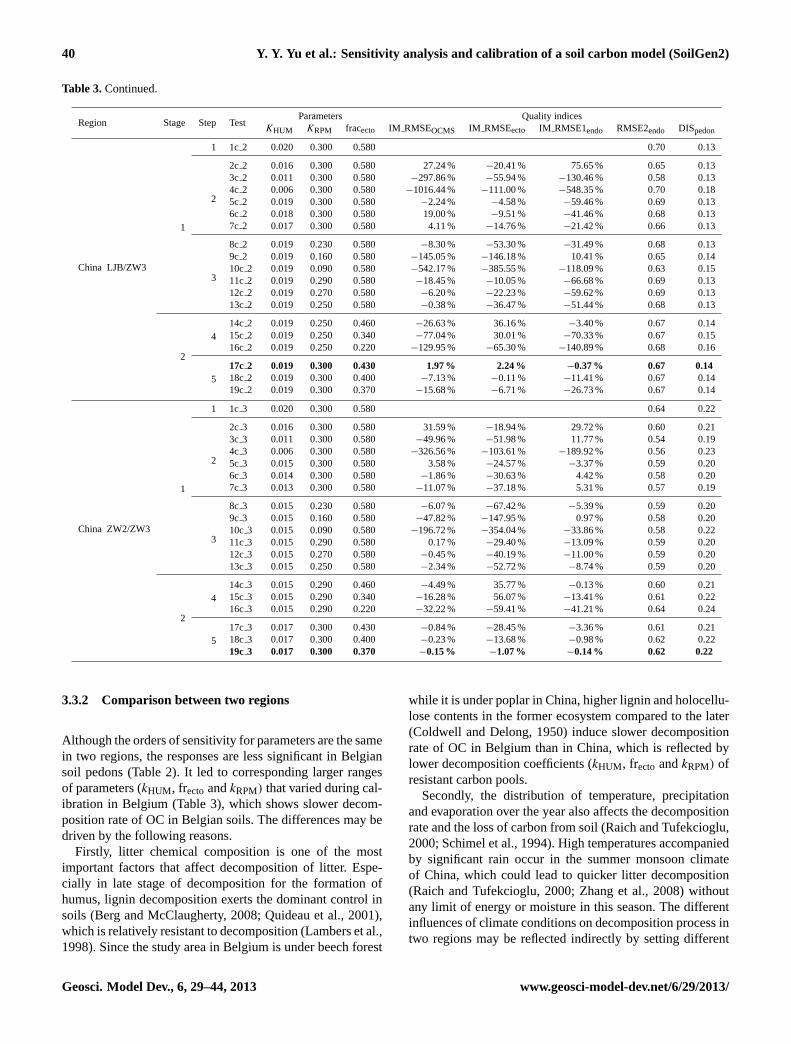
Based on 67 and 57 test simulations, three sets of calibratedparameters were obtained for Belgium and China, respec-tively. Table 3 gives the model parameters in calibrationstests. Results comparing simulated and measured OC byeight quality indices are given in Figs. 4 and 5 and Table3, with lower absolute values of them indicating better simu-lated results.

In the stage of calibration (steps 2 and 3 in Table 3), tests(1bs and 1cs) with default values of parameters in SoilGen2(step 1 in Table 3) showed that simulated total OC mass waslower than measured ones in both regions with larger de-viations in Belgium than in China (Fig. 4d–f and j–l). Thedifferences in total OC mass were minimized by decreas-ing the most sensitive parameterkHUM and the second sen-sitive parameterkRPM during the first calibration stage (Ta-ble 3). The IMRMSEOCMS became much lower than 5 %,when kHUM values were set as 0.0061–0.0065 and 0.014–0.019, andkRPM values were 0.27–0.29 and 0.25–0.29 inBelgium and China, respectively. The RMSEOCMS resultingfrom these simulations served as target quality for the secondstage of calibration.

The following calibrations for both regions were to ad-just the distribution of OC in ectorganic (overestimation

in stage 1) and endorganic (underestimation) layers. Basedon tests in steps 4 in both regions with variation offrecto, it was revealed that the decrease of frecto couldalso increase the amount of OC mass in both layers (Ta-ble 3). In order to reduce this effect and the values ofRMSEecto and RMSEendo simultaneously,kHUM and kRPMwere increased slightly (steps 5 and 6 in Table 3). Thebest results were finally obtained in Test21b1, Test22b2and Test22b3 in Belgium and Test18c1, Test17c2 andTest19c3 in China with the following combination of pa-rameters (Belgium,kHUM = 0.0065–0.0074,kRPM = 0.27–0.27 and frecto= 0.30–0.38; China,kHUM = 0.016–0.019,kRPM = 0.30–0.30 and frecto= 0.37–0.43), with the lowestvalues of IMRMSEecto and IM RMSEendoat the same timewhile the RMSEOCMS remained close to the value reached inthe first stage of the calibration.

Above tests were further confirmed as the best calibrationresults by comparing eight quality indices synthetically (Ta-ble 3 and Fig. 4), because the indices of them all belong tothe lower ones in all tests of two regions. Figure 5 furthershows that the simulated vertical distributions of OC contentare also similar to measured ones visually.

The comparisons between measured and simulated OC ofthe validation pedons are given in Fig. 6. Two groups of OCmass are evenly distributed along 1: 1 line (Fig. 6a), andRMSEOCMS values of pedons are all less than 12 % of thetotal OC mass. Furthermore, the consistency is also evidentin vertical distributions of OC content (Fig. 6b–g).

This two-stage calibration approach was repeatedthree times, always calibrating with two pedons in a regionwhile checking the quality with the third pedon. Resultsindicate that the calibration results are fairly stable andindependent on the subset of two pedons chosen for thecalibration. This suggests that the calibrated parameters areapplicable to other soil pedons in similar climate conditions.



Table 3.Model parameters in the organic C-module in SoilGen2 and quality indices of one group of pedons during the calibration in Belgiumand China. Bold numbers indicate the best calibration results for each group of pedons.

Region Stage Step TestParameters Quality indices

KHUM KRPM fracecto IM RMSEOCMS IM RMSEecto IM RMSE1endo RMSE2endo DISpedon

Belgium N/P

1

1 1b 1 0.0200 0.3000 0.5800 0.79 0.29

2

2b 1 0.0160 0.3000 0.5800 10.84 % 57.65 % 7.47 % 0.74 0.273b 1 0.0110 0.3000 0.5800 24.40 % −140.93 % 17.85 % 0.63 0.234b 1 0.0060 0.3000 0.5800 56.27 % −487.93 % 49.39 % 0.56 0.215b 1 0.0070 0.3000 0.5800 −13.44 % −393.85 % −15.15 % 0.54 0.206b 1 0.0065 0.3000 0.5800 −6.79 % −438.74 % −10.07 % 0.58 0.217b 1 0.0061 0.3000 0.5800 −0.25 % −477.72 % −3.84 % 0.59 0.22

3

8b 1 0.0061 0.2300 0.5800 −1.01 % −591.30 % 1.19 % 0.56 0.219b 1 0.0061 0.1600 0.5800 −11.99 % −804.60 % 5.13 % 0.56 0.2110b 1 0.0061 0.0900 0.5800 −47.23 % −1350.40 % 8.54 % 0.58 0.2111b 1 0.0061 0.2900 0.5800 −0.23 % −490.58 % −16.20 % 0.55 0.2112b 1 0.0061 0.2700 0.5800 0.07 % −519.16 % −15.47 % 0.55 0.2113b 1 0.0061 0.2500 0.5800 −0.18 % −552.33 % −14.64 % 0.55 0.21

2

414b 1 0.0061 0.2700 0.4600 −1.14 % −201.11 % −1.49 % 0.54 0.2015b 1 0.0061 0.2700 0.3400 −4.24 % −48.53 % −6.34 % 0.56 0.2116b 1 0.0061 0.2700 0.2200 −8.19 % −360.45 % −22.66 % 0.61 0.23

5

17b 1 0.0070 0.2700 0.5800 −10.96 % −435.24 % −28.89 % 0.54 0.2018b 1 0.0068 0.2700 0.5800 −7.91 % −452.73 % −26.15 % 0.54 0.2019b 1 0.0066 0.2700 0.5800 −4.92 % −470.85 % −23.27 % 0.54 0.2020b 1 0.0065 0.2700 0.5800 −3.51 % −480.16 % −21.78 % 0.54 0.20

621b 1 0.0065 0.2700 0.3800 −0.18 % 0.00 % −0.22 % 0.53 0.2022b 1 0.0065 0.2700 0.3700 −0.15 % −6.99 % −0.17 % 0.53 0.2023b 1 0.0065 0.2700 0.3600 −0.14 % −24.19 % −0.32 % 0.53 0.20

Belgium N/S

1

1 1b 2 0.0200 0.3000 0.5800 0.86 0.28

2

2b 2 0.0160 0.3000 0.5800 11.42 % −27.94 % 7.35 % 0.81 0.263b 2 0.0110 0.3000 0.5800 25.47 % −96.30 % 17.53 % 0.69 0.224b 2 0.0060 0.3000 0.5800 44.42 % −244.62 % 49.38 % 0.54 0.185b 2 0.0070 0.3000 0.5800 −3.14 % −203.86 % −15.25 % 0.55 0.186b 2 0.0065 0.3000 0.5800 2.54 % −223.28 % −10.61 % 0.56 0.197b 2 0.0061 0.3000 0.5800 1.71 % −240.19 % −4.36 % 0.57 0.19

3

8b 2 0.0065 0.2300 0.5800 −3.24 % −272.64 % −5.12 % 0.54 0.189b 2 0.0065 0.1600 0.5800 −11.58 % −366.05 % 0.41 % 0.53 0.1810b 2 0.0065 0.0900 0.5800 −46.70 % −607.04 % 12.76 % 0.53 0.1711b 2 0.0065 0.2900 0.5800 −2.98 % −228.85 % −20.94 % 0.54 0.1812b 2 0.0065 0.2700 0.5800 −2.75 % −241.25 % −20.18 % 0.54 0.1813b 2 0.0065 0.2500 0.5800 −2.78 % −255.67 % −19.31 % 0.54 0.18

2

414b 2 0.0065 0.2700 0.4600 −3.25 % −108.73 % −4.21 % 0.50 0.1715b 2 0.0065 0.2700 0.3400 −4.92 % 3.25 % 2.87 % 0.49 0.1616b 2 0.0065 0.2700 0.2200 −7.46 % −20.85 % −12.88 % 0.51 0.17

517b 2 0.0072 0.2700 0.5800 −7.71 % −217.70 % −32.77 % 0.56 0.1818b 2 0.0070 0.2700 0.5800 −5.67 % −225.01 % −30.17 % 0.55 0.1819b 2 0.0068 0.2700 0.5800 −4.01 % −232.59 % −27.43 % 0.55 0.18

620b 2 0.0070 0.2700 0.3200 −2.88 % 13.86 % 0.21 % 0.48 0.1621b 2 0.0070 0.2700 0.3100 −2.87 % 1.86 % 0.31 % 0.48 0.1622b 2 0.0070 0.2700 0.3000 −2.86 % 0.32 % 0.11 % 0.48 0.16

3.3 Comparison

3.3.1 Comparison with former studies

Our results of sensitivity analysis are in accordance with for-mer studies on RothC model in surface forest soils (Pauland Polglase, 2004; Paul et al., 2003), which indicated thatchange in soil carbon is particularly sensitive to the decom-position rates of HUM, RPM and BIO pools. Comparing that

only the relative importance of the parameters was shown informer analysis (Paul and Polglase, 2004; Paul et al., 2003),a quantitative evaluation of their importance is given in ourstudy and the especially significant sensitivity ofkHUM is re-vealed.

The calibrated values of parameters (kHUM andkRPM) inour study all fall into the logical range of former calibrationsfor RothC model (Shirato et al., 2004; Skjemstad et al., 2004;Todorovic et al., 2010), covering various climate conditions



Table 3.Continued.



Belgium P/S

1

1 1b 3 0.0200 0.3000 0.5800 0.65 0.33

2

2b 3 0.0160 0.3000 0.5800 12.83 % −19.21 % 8.23 % 0.60 0.313b 3 0.0110 0.3000 0.5800 28.87 % −75.60 % 19.73 % 0.50 0.254b 3 0.0060 0.3000 0.5800 38.04 % −208.78 % 56.58 % 0.48 0.235b 3 0.0070 0.3000 0.5800 9.76 % −171.64 % −17.93 % 0.44 0.226b 3 0.0065 0.3000 0.5800 1.83 % −189.30 % −15.61 % 0.51 0.247b 3 0.0061 0.3000 0.5800 −3.59 % −204.73 % −8.58 % 0.53 0.24

3

8b 3 0.0065 0.2300 0.5800 −8.67 % −234.43 % −6.18 % 0.45 0.229b 3 0.0065 0.1600 0.5800 −24.37 % −320.37 % 0.30 % 0.46 0.2210b 3 0.0065 0.0900 0.5800 −67.16 % −543.48 % 13.09 % 0.49 0.2311b 3 0.0065 0.2900 0.5800 −2.67 % −194.38 % −22.63 % 0.45 0.2212b 3 0.0065 0.2700 0.5800 −4.15 % −205.70 % −21.76 % 0.45 0.2213b 3 0.0065 0.2500 0.5800 −6.12 % −218.88 % −20.75 % 0.45 0.22

2

414b 3 0.0065 0.2900 0.4600 −6.50 % −78.31 % −3.46 % 0.43 0.2115b 3 0.0065 0.2900 0.3400 −11.11 % 3.93 % −12.10 % 0.43 0.2116b 3 0.0065 0.2900 0.2200 −16.07 % −41.64 % −31.49 % 0.48 0.23

517b 3 0.0074 0.2700 0.5800 −4.54 % −178.78 % −35.91 % 0.43 0.2218b 3 0.0072 0.2700 0.5800 −2.16 % −185.19 % −33.07 % 0.43 0.2219b 3 0.0070 0.2700 0.5800 −0.67 % −191.85 % −30.06 % 0.44 0.22

620b 3 0.0074 0.2700 0.3500 −0.53 % 0.48 % −1.45 % 0.38 0.2021b 3 0.0074 0.2700 0.3400 −0.50 % 1.97 % −0.17 % 0.38 0.2022b 3 0.0074 0.2700 0.3300 −0.49 % 0.88 % 0.56 % 0.38 0.20

China LJB/ZW2

1

1 1c 1 0.020 0.300 0.580 0.68 0.18

2

2c 1 0.016 0.300 0.580 42.57 % −23.22 % 32.20 % 0.62 0.163c 1 0.011 0.300 0.580 −37.79 % −63.49 % 13.72 % 0.52 0.154c 1 0.006 0.300 0.580 −301.80 % −125.70 % −185.47 % 0.56 0.175c 1 0.015 0.300 0.580 8.72 % −30.10 % −4.52 % 0.60 0.166c 1 0.014 0.300 0.580 3.08 % −37.50 % 4.18 % 0.58 0.167c 1 0.013 0.300 0.580 −6.69 % −45.48 % 6.13 % 0.56 0.15

3

8c 1 0.014 0.230 0.580 −11.02 % −93.16 % −0.33 % 0.57 0.169c 1 0.014 0.160 0.580 −58.42 % −198.38 % 0.13 % 0.54 0.1510c 1 0.014 0.090 0.580 −205.00 % −468.32 % −43.35 % 0.51 0.1611c 1 0.014 0.290 0.580 −0.25 % −43.79 % −5.44 % 0.58 0.1612c 1 0.014 0.270 0.580 −1.81 % −57.74 % −3.76 % 0.58 0.1613c 1 0.014 0.250 0.580 −5.25 % −74.04 % −2.07 % 0.57 0.16

2

414c 1 0.014 0.290 0.460 −10.88 % 39.77 % −0.75 % 0.56 0.1615c 1 0.014 0.290 0.340 −28.32 % 22.36 % −22.90 % 0.55 0.1716c 1 0.014 0.290 0.220 −48.04 % −80.84 % −54.20 % 0.56 0.18

517c 1 0.016 0.300 0.430 −1.11 % 8.76 % 1.22 % 0.58 0.1618c 1 0.016 0.300 0.400 −0.99 % 0.53 % 0.05 % 0.58 0.1619c 1 0.016 0.300 0.370 −1.56 % −9.06 % −1.04 % 0.57 0.17

and soil types, They are lower than default values in RothCmodel, which was originally developed and parameterized insurface agricultural soils (0–30 cm) (Jenkinson, 1990). Thedifference may be attributed to following aspects: firstly, de-composition in agricultural soils is faster than that in forestsoils because of its lower lignin content in litter (Lambers etal., 1998) and more favorable micro-climate conditions fordecomposition induced by human disturbance (Schlesingerand Andrews, 2000); secondly, carbon at deeper depth (1.5–2.5 m in our study) is older than that near the surface, indi-cating that it has a greater resistance to decomposition or thatthe environment at depth is less favorable for decompositionprocesses (Swift, 2001).

The calibrated frecto is lower than the default value (0.58)in SoilGen2 based on measured data (Kononova, 1975). Inrealistic soil carbon cycle process, part of litter carbon poolin ectorganic layer leaches to endorganic layers in the formof dissolved organic carbon (DOC). However, this process isnot simulated in SoilGen2, while only little carbon is beingexchanged between two layers by bioturbation in the model.Therefore, frecto, as the ratio of carbon pool in ectorganiclayer to the total pool, was expected to be lower than theliterature value as this decrease mimics the effect of DOC-leaching.



Table 3.Continued.



China LJB/ZW3

1

1 1c 2 0.020 0.300 0.580 0.70 0.13

2

2c 2 0.016 0.300 0.580 27.24 % −20.41 % 75.65 % 0.65 0.133c 2 0.011 0.300 0.580 −297.86 % −55.94 % −130.46 % 0.58 0.134c 2 0.006 0.300 0.580 −1016.44 % −111.00 % −548.35 % 0.70 0.185c 2 0.019 0.300 0.580 −2.24 % −4.58 % −59.46 % 0.69 0.136c 2 0.018 0.300 0.580 19.00 % −9.51 % −41.46 % 0.68 0.137c 2 0.017 0.300 0.580 4.11 % −14.76 % −21.42 % 0.66 0.13

3

8c 2 0.019 0.230 0.580 −8.30 % −53.30 % −31.49 % 0.68 0.139c 2 0.019 0.160 0.580 −145.05 % −146.18 % 10.41 % 0.65 0.1410c 2 0.019 0.090 0.580 −542.17 % −385.55 % −118.09 % 0.63 0.1511c 2 0.019 0.290 0.580 −18.45 % −10.05 % −66.68 % 0.69 0.1312c 2 0.019 0.270 0.580 −6.20 % −22.23 % −59.62 % 0.69 0.1313c 2 0.019 0.250 0.580 −0.38 % −36.47 % −51.44 % 0.68 0.13

2

414c 2 0.019 0.250 0.460 −26.63 % 36.16 % −3.40 % 0.67 0.1415c 2 0.019 0.250 0.340 −77.04 % 30.01 % −70.33 % 0.67 0.1516c 2 0.019 0.250 0.220 −129.95 % −65.30 % −140.89 % 0.68 0.16

517c 2 0.019 0.300 0.430 1.97 % 2.24 % −0.37 % 0.67 0.1418c 2 0.019 0.300 0.400 −7.13 % −0.11 % −11.41 % 0.67 0.1419c 2 0.019 0.300 0.370 −15.68 % −6.71 % −26.73 % 0.67 0.14

China ZW2/ZW3

1

1 1c 3 0.020 0.300 0.580 0.64 0.22

2

2c 3 0.016 0.300 0.580 31.59 % −18.94 % 29.72 % 0.60 0.213c 3 0.011 0.300 0.580 −49.96 % −51.98 % 11.77 % 0.54 0.194c 3 0.006 0.300 0.580 −326.56 % −103.61 % −189.92 % 0.56 0.235c 3 0.015 0.300 0.580 3.58 % −24.57 % −3.37 % 0.59 0.206c 3 0.014 0.300 0.580 −1.86 % −30.63 % 4.42 % 0.58 0.207c 3 0.013 0.300 0.580 −11.07 % −37.18 % 5.31 % 0.57 0.19

3

8c 3 0.015 0.230 0.580 −6.07 % −67.42 % −5.39 % 0.59 0.209c 3 0.015 0.160 0.580 −47.82 % −147.95 % 0.97 % 0.58 0.2010c 3 0.015 0.090 0.580 −196.72 % −354.04 % −33.86 % 0.58 0.2211c 3 0.015 0.290 0.580 0.17 % −29.40 % −13.09 % 0.59 0.2012c 3 0.015 0.270 0.580 −0.45 % −40.19 % −11.00 % 0.59 0.2013c 3 0.015 0.250 0.580 −2.34 % −52.72 % −8.74 % 0.59 0.20

2

414c 3 0.015 0.290 0.460 −4.49 % 35.77 % −0.13 % 0.60 0.2115c 3 0.015 0.290 0.340 −16.28 % 56.07 % −13.41 % 0.61 0.2216c 3 0.015 0.290 0.220 −32.22 % −59.41 % −41.21 % 0.64 0.24

517c 3 0.017 0.300 0.430 −0.84 % −28.45 % −3.36 % 0.61 0.2118c 3 0.017 0.300 0.400 −0.23 % −13.68 % −0.98 % 0.62 0.2219c 3 0.017 0.300 0.370 −0.15 % −1.07 % −0.14 % 0.62 0.22

3.3.2 Comparison between two regions

Although the orders of sensitivity for parameters are the samein two regions, the responses are less significant in Belgiansoil pedons (Table 2). It led to corresponding larger rangesof parameters (kHUM , frectoandkRPM) that varied during cal-ibration in Belgium (Table 3), which shows slower decom-position rate of OC in Belgian soils. The differences may bedriven by the following reasons.

Firstly, litter chemical composition is one of the mostimportant factors that affect decomposition of litter. Espe-cially in late stage of decomposition for the formation ofhumus, lignin decomposition exerts the dominant control insoils (Berg and McClaugherty, 2008; Quideau et al., 2001),which is relatively resistant to decomposition (Lambers et al.,1998). Since the study area in Belgium is under beech forest

while it is under poplar in China, higher lignin and holocellu-lose contents in the former ecosystem compared to the later(Coldwell and Delong, 1950) induce slower decompositionrate of OC in Belgium than in China, which is reflected bylower decomposition coefficients (kHUM , frecto andkRPM) ofresistant carbon pools.

Secondly, the distribution of temperature, precipitationand evaporation over the year also affects the decompositionrate and the loss of carbon from soil (Raich and Tufekcioglu,2000; Schimel et al., 1994). High temperatures accompaniedby significant rain occur in the summer monsoon climateof China, which could lead to quicker litter decomposition(Raich and Tufekcioglu, 2000; Zhang et al., 2008) withoutany limit of energy or moisture in this season. The differentinfluences of climate conditions on decomposition process intwo regions may be reflected indirectly by setting different



(a) (b) (c)

(d) (e) (f)

(g) (h) (i)

0

10

20

30

40

50

60

70

0 2 4 6 8 10 12 14 16 18 20 22 24

RMSE OCMS, N/P

RMSE ecto, N/P

RMSE1 endo, N/P

0

10

20

30

40

50

60

70

0 2 4 6 8 10 12 14 16 18 20 22 24

RMSE OCMS, N/SRMSE ecto, N/SRMSE endo, N/S

0

10

20

30

40

50

60

0 2 4 6 8 10 12 14 16 18 20 22 24

RMSE OCMS, P/SRMSE ecto, P/SRMSE endo. P/S

OC

(ton

ha

)-1O

C (t

on h

a )-1

Yu et al., Fig. 4

Test number Test number Test number

0

10

20

30

40

50

60

70

80

0 2 4 6 8 10 12 14 16 18 20

RMSE OCMS, LJB/ZW2

RMSE ecto, LJB/ZW2

RMSE endo, LJB/ZW2

0

10

20

30

40

50

60

70

80

90

0 2 4 6 8 10 12 14 16 18 20

RMSE OCMS, LJB/ZW3

RMSE ecto, LJB/ZW3

RMSE endo, LJB/ZW3

0

10

20

30

40

50

60

70

80

0 2 4 6 8 10 12 14 16 18 20

RMSE OCMS. ZW2/ZW3

RMSE ecto, ZW2/ZW3

RMSE endo, ZW2/ZW3

-60

-40

-20

0

20

40

60

80

0 2 4 6 8 10 12 14 16 18 20 22 24

MD OCMS, P/SMD ecto, P/SMD endo, P/S

-60

-40

-20

0

20

40

60

80

0 2 4 6 8 10 12 14 16 18 20 22 24

MD OCMS, N/SMD ecto, N/SMD endo, N/S

-60

-40

-20

0

20

40

60

80

0 2 4 6 8 10 12 14 16 18 20 22 24

MD OCMS, N/PMD ecto, N/PMD endo, N/P

-90

-70

-50

-30

-10

10

30

50

0 2 4 6 8 10 12 14 16 18 20

MD OCMS, ZW2/ZW3

MD ecto, ZW2/ZW3

MD endo, ZW2/ZW3-90

-70

-50

-30

-10

10

30

50

0 2 4 6 8 10 12 14 16 18 20

MD OCMS, LJB/ZW3

MD ecto, LJB/ZW3

MD endo, LJB/ZW3-80

-60

-40

-20

0

20

40

60

0 2 4 6 8 10 12 14 16 18 20

MD OCMS, LJB/ZW2MD ecto, LJB/ZW2MD endo, LJB/ZW2




OC

(ton

ha

)-1O

C (t

on h

a )-1

(j) (k) (l)

Fig. 4. Quality indices for calibration results.(a) RMSE of aver-age OC mass in N/P pedons in Belgium;(b) RMSE of average OCmass in N/S pedons in Belgium;(c) RMSE of average OC mass inP/S pedons in Belgium;(d) MD of average OC mass in N/P pedonsin Belgium;(e)MD of average OC mass in N/S pedons in Belgium;(f) MD of average OC mass in P/S pedons in Belgium;(g) RMSEof average OC mass in LJB/ZW2 pedons in China;(h) RMSE ofaverage OC mass in LJB/ZW3 pedons in China;(i) RMSE of av-erage OC mass in ZW2/ZW3 pedons in China;(j) MD of averageOC mass in LJB/ZW2 pedons in China;(k) MD of average OCmass in LJB/ZW3 pedons in China;(l) MD of average OC mass inZW2/ZW3 pedons in China.

values of these parameters, because just decomposition co-efficients (kHUM , frecto andkRPM) of soil carbon pools werecalibrated in this study, and not the mechanisms that mimicthe effect of temperature and moisture on decomposition.

Finally, because the effect of some soil properties (e.g.,CaCO3 content, pH) on OC cycle is not incorporated in Soil-Gen2 (except clay and water content), the difference of theseproperties in two regions may explain part of the variation incalibrated parameters. This relationship could be quantifiedvia regression analysis based on many simulated and cali-brated plots. However, the small number of calibrated plotsin our study does not allow for such analysis.

(d)LJB/ZW2, China (e)LJB/ZW3, China (f)ZW2/ZW3, China

(a)N/P, Belgium (b)N/S, Belgium (c)P/S, Belgium

Averagesimulated OCAveragemeasured OCMin and Maxsimulated OC

OC (%)

Dep

th (c

m)

Dep

th (c

m)

Yu et al., Fig. 5

010203040

5060708090

100

0 10 20 30 400

1020

3040506070

8090

100

0 10 20 300

1020

3040506070

8090

100

0 10 20 30

01020

3040506070

8090

100

0 5 10 150

1020

3040506070

8090

100

0 5 10 150

1020

3040506070

8090

100

0 5 10 15

Fig. 5. Comparison of vertical distribution of simulated vs. mea-sured OC content in soil pedons.(a) N/P pedons in Belgium;(b)N/S pedons in Belgium;(c) P/S pedons in Belgium;(d) LJB/ZW2pedons in China;(e) LJB/ZW3 pedons in China;(f) ZW2/ZW3 pe-dons in China. Min is minimal value while Max is maximal value.

In addition, the different calibrated results in Belgium andChina indicate that future calibrations are needed for distinctclimate conditions, possibly for different soil types as well,and uncertainty bandwidths of calibrated parameters shouldbe given. The current study however does not allow a cer-tain statement on this topic as only a few soil type/climatecombinations have been explored.

4 Conclusions

Sensitivity analysis based on the Morris method shows thatkHUM , frecto andkRPM are the three most important parame-ters in SoilGen2 to affect change of OC both in Belgian andChinese soil pedons. The sensitivity orders of the parametersfollow the same pattern in the two regions, but the values ofelementary effects differ.

According to the results of sensitivity analysis, SoilGen2parameters are calibrated by decreasingkHUM , frecto andkRPM. The final results are obtained by the following combi-nation of parameters:kHUM = 0.0065–0.0074,kRPM = 0.27–0.27 and frecto= 0.30–0.38 in Belgium andkHUM = 0.016–0.019, kRPM = 0.30–0.30 and frecto= 0.37–0.43 in China.The less significant sensitivity of parameters in the sensitivityanalysis and larger variation of parameters during calibrationin Belgium compared to China may be attributed to their dis-tinct vegetation types and climate conditions.



(e)LJB, China (f)ZW2, China (g)ZW3, China

Yu et al., Fig. 6

(a)

Sim

ulat

ed O

C (t

on h

a )-1

Measured OC (ton ha ) -1

0

50

100

150

200

0 50 100 150 200

Total OC, BelgiumTotal OC, Chinaecto OC, Belgiumendo OC, Belgiumecto OC, Chinaendo OC, China1:1 line

Dep

th (c

m)

(b)N, Belgium (c)P, Belgium (d)S, Belgium

Simulated OCMeasured OC

OC (%)

0102030405060708090

100

0 10 20 300

102030405060708090

100

0 10 20 30

0102030405060708090

100

0 5 10 150

102030405060708090

100

0 5 10 150

102030405060708090

100

0 5 10 15 20

0102030405060708090

100

0 10 20 30 40

Dep

th (c

m)

Fig. 6. Comparison of measured and simulated OC based on soilpedons for validation in Belgium and China.(a) OC mass in Bel-gium and China;(b) OC content of N pedon in Belgium;(c) OCcontent of P pedon in Belgium;(d) OC content of S pedon in Bel-gium; (e) OC content of LJB pedon in China;(f) OC content ofZW2 pedon in China;(g) OC content of ZW3 pedon in China.

The calibrated parameters follow the law that OC in deepersoil layers is more resistant to decomposition than in surfacesoil layers, which is induced by the age of carbon and an un-favorable environment for soil micro-organisms in the deeperlayers. This indicates that the calibration allows better sim-ulation of carbon storage in the whole soil pedon. The cali-brated SoilGen2 will be the base for quantitative soil carbonpool reconstruction based on the application of it to loess-soil

sequences deposited in China in future studies, which willoffer an opportunity to understand the mechanism of carboncycle at geological timescale.

Acknowledgements.This work was supported by the CAS StrategicPriority Research Program Grant No. XDA05120000, the NationalNatural Science Foundation of China (No: 41102222, 41071055)and LiSUM project of Erasmus Mundus External CooperationWindow. Thanks are extended to Arne Verstraeten and NathalieCools of the Research Institute for Nature and Forest, Belgium, forthe measured data of litter input in Sonian Forest region.

Edited by: D. Lawrence

References

Berg, B. and McClaugherty, C. (Eds.): Plant Litter: decomposition,humus formation, carbon Sequestration, 2nd Edn., Springer-Verlag, Berlin-Heidelberg, Germany, 2008.

Campolongo, F., Kleijnen, J., and Andres, T.: Screening methods,in: Sensitivity analysis, edited by: Saltelli, A., Chan, K., andScott, M., Wiley and Sons, Chichester, UK, 65–80, 2000.

Cao, Y., Zhao, Z., Qu, M., Cheng, X. Y., and Wang D. H.: Effects ofRobinia pseudoacacia roots on deep soil moisture status, Chin. J.Appl. Ecol., 17, 765–768, 2006.

Coldwell, B. B. and DeLong, W. A.: Studies of the composition ofdeciduous forest tree leaves before and after partial decomposi-tion, Sci. Agric., 30, 456–466, 1950.

Coleman, K. and Jenkinson, D. S.: RothC-26.3 a model forthe turnover of carbon in soil, available at:http://www.rothamsted.bbsrc.ac.uk/aen/carbon/download.htm(last access:10 June 2012), 2005.

Coleman, K., Jenkinson, D. S., Crocker, G. J., Grace, P. R., Klır,J., Korschens, M., Poulton, P. R., and Richter D. D.: Simulat-ing trends in soil organic carbon in long-term experiments usingRothC-26.3, Geoderma, 81, 29–44, 1997.

Cui, L. J., Liang, Z. S., Han, R. L., and Yang, J. W.: Biomass soiland root system distribution characteristics of Seabuckthorn×

Poplar mixed forest, Sci. Silv. Sin., 39, 1–7, 2003.Davis, B. A. S., Brewer, S., Stevenson, A. C., Guiot, J., and Data

Contributors: The temperature of Europe during the Holocenereconstructed from pollen data, Quaternary Sci. Rev., 22, 1701–1716, 2003.

De Wit, H. A., Palosuo, T., Hylen, G., and Liski, J.: A carbon bud-get of forest biomass and soils in southeast Norway, Forest Ecol.Manag., 225, 15–26, 2006.

Doherty, J. (Ed.): PEST: model independent parameter estimationuser manual, Fifth Edition, Watermark Numerical Computing,Brisbane, Australia, 2004.

Falkowski, P., Scholes, R. J., Boyle, E., Canadell, J., Canfield,D., Elser, J., Gruber, N., Hibbard, K., Hogberg, P., Linder, S.,Mackenzie, F. T., Moore III, B., Pedersen, T., Rosenthal, Y.,Seitzinger, S., Smetacek, V., and Steffen, W.: The global carboncycle: a test of our knowledge of earth as a system, Science, 290,291–296, 2000.

Finke, P. A.: Modeling the genesis of Luvisols as a function of to-pographic position in loess parent material, Quaternary Int., 265,3–17, 2012.


http://www.rothamsted.bbsrc.ac.uk/aen/carbon/download.htm

http://www.rothamsted.bbsrc.ac.uk/aen/carbon/download.htm


Finke, P. A. and Hutson, J.: Modelling soil genesis in calcareousloess, Geoderma, 145, 462–479, 2008.

Gobat, J. M., Aragno, M., and Matthey, W. (Eds): The Living Soil:Fundamentals of Soil Science and Soil Biology, Science Publish-ers Inc., NH, USA, 2004.

Gong, Z. T., Chen, Z. C., and Zhang, G. L.: World reference basefor soil resources (WRB): Establishment and development, Soils,35, 271–278, 2003.

Gower, J. C.: A general coefficient of similarity and some of itsproperties, Biometrics, 27, 623–637, 1971.

Grievank, A. and Walter, A. (Eds.): Evaluating derivatives, prin-ciples and techniques of algorithmic differentiation, SIAM,Philadelphia, USA, 2008.

Guo, Z. T., Ruddiman, W. F., Hao, Q. Z., Wu, H. B., Qiao, Y. S.,Zhu, R. X., Peng, S. Z., Wei, J. J., Yuan, B. Y., and Liu, T. S.:Onset of Asian desertification by 22 Myr ago inferred from loessdeposits in China, Nature, 416, 159–163, 2002.

Hu, X. N., Zhao, Z., Yuan, Z. F., Li, J., Guo, M. C., and Wang, D.H.: A model for fine root growth of Robinia pseudoacacia in theLoess Plateau, Sci. Silv. Sin., 46, 126–132, 2010.

IUSS Working Group WRB: World Reference Base for Soil Re-sources 2006, in: World Soil Resources Report No. 103, 2ndEdn., FAO, Rome, Italy, 2006.

Jenkinson, D. S.: The turnover of organic carbon and nitrogen insoil, Philos. T. R. Soc. Lond., 329, 361–368, 1990.

Jenkinson, D. S. and Coleman, K.: Calculating the annual input oforganic matter to soil from measurements of total organic carbonand radiocarbon, Eur. J. Soil Sci., 45, 167–174, 1994.

Jenny, H.: Derivation of state factor equations of soils and ecosys-tems, Soil Sci. Soc. Am. Pro., 25, 385–388, 1961.

Jensen, L. S., Mueller, T., Nielsen, N. E., Hansen, S., Crocker, G. J.,Grace, P. R., Klir, J., Korschens, M., and Poulton, P. R.: Simulat-ing trends in soil organic carbon in long-term experiments usingthe soil-plant-atmosphere model DAISY, Geoderma, 81, 5–28,1997.

Kelly, R. H., Parton W. J., Crocker, G. J., Graced, P. R., Klir, J.,Korschens, M., Poulton, P. R., and Richter, D. D.: Simulatingtrends in soil organic carbon in long-term experiments using thecentury model, Geoderma, 81, 75–90, 1997.

Kirkby, M. J.: Soil development models as a component of slopemodels, Earth Surf. Proc. Landf., 2, 203–230, 1977.

Kononova, M. M.: Humus of virgin and cultivated soils, in: Soilcomponents. I. Organic Components, edited by: Gieseling, J. E.,Springer, Berlin, Germany, 475–526, 1975.

Kukla, G. J.: Correlation of Chinese, European and American loessseries with deep-sea sediments, in: Aspects of loess research,edited by: Liu, T. S., China Ocean Press, Beijing, China, 27–38,1987.

Lal, R.: Soil Carbon sequestration impacts on global climate changeand food security, Science, 304, 1623–1627, 2004.

Lambers, H., Chapin, F. S., and Pons, T. L. (Eds.): Plant Physiolog-ical Ecology, Springer-Verlag New York Inc, New York, USA,1998.

Langohr, R. and Sanders, J.: The Belgian loess belt in the last20,000 years: evolution of soils and relief in the Zonien forest,in: Soils and Quaternary Landscape Evolution, edited by: Board-man, J., Wiley, Chichester, UK, 359–371, 1985.

Li, C. S., Frolking, S., Crocker, G. J., Grace, P. R., Klir, J., Korchens,M., and Poulton, P. R.: Simulating trends in soil organic carbon

in long-term experiments using the DNDC model, Geoderma, 81,45–60, 1997.

Liu, T. S. (Ed.): Loess and the Environment, Science Press, Beijing,China, 1985.

Liu, Y.: The relationship between community biomass and soilmoisture, soil nutrient in ZIwuling typical forests, Master Degreethesis, Northwest Agriculture and Forest University, Yangling,China, 2007.

Mermut, A. R., Amundson, R., and Cerling, T. E.: The use of sta-ble isotopes in studying carbonate dynamics in soils, in: GlobalClimate Change and Pedogenic Carbonates, edited by: Lal, R.,Kimble, J. M., Eswaran, H., and Stewart, B. A. (Eds), CRC Press,Boca Raton, USA, 65–85, 2000.

Minasny, B. and McBratney, A. B.: A rudimentary mechanisticmodel for soil production and landscape development, Geo-derma, 90, 3–21, 1999.

Minasny, B. and McBratney, A. B.: A rudimentary mechanisticmodel for soil production and landscape development II. A two-dimensional model incorporating chemical weathering, Geo-derma, 103, 161–179, 2001.

Minasny, B., McBratney, A. B., and Salvador-Blanes, S.: Quantita-tive models for pedogenesis: a review, Geoderma, 144, 140–157,2008.

Morris, M. D.: Factorial sampling plans for preliminary computa-tional experiments, Technometrics, 33, 161–174, 1991.

Oakley, J. and O’Hagan, A.: Probabilistic sensitivity analysis ofcomplex models: a Bayesian approach, J. Roy. Stat. Soc. B., 66,751–769, 2004.

Parton, W. J., Schimel, D. S., Cole, C. V., and Ojima, D. S.: Analysisof factors controlling soil organic matter levels in Great Plainsgrasslands, Soil Sci. Soc. Am. J., 51, 1173–1179, 1987.

Paul, K. I. and Polglase, P. J.: Calibration of the RothC model toturnover of soil carbon under eucalypts and pines, Aust. J. SoilRes., 42, 883–895, 2004.

Paul, K. I., Polglase, P. J., and Richards, G. P.: Sensitivity analysisof predicted change in soil carbon following afforestation, Ecol.Model., 164, 137–152, 2003.

Post, W. F., Peng, T. H., Emanuel, W. R., King, A. W., Dale, V. H.,and DeAngelis, D. L.: The global carbon cycle, Am. Sci., 78,310–326, 1990.

Quideau, S. A., Chadwick, O. A., Benesi, A., Graham, R. C., andAnderson, M. A.: A direct link between forest vegetation typeand soil organic matter composition, Geoderma, 104, 41–60,2001.

Raich, J. W. and Tufekcioglu, A.: Vegetation and soil respiration:correlations and controls, Biogeochemistry, 48, 71–90, 2000.

Saltelli, A., Chan, K., and Scott, M. (Eds.): Sensitivity analysis, Wi-ley and Sons, Chichester, UK, 2000.

Saltelli, A., Ratto, M., Tarantola, S., and Campolongo, F.: Sensitiv-ity analysis for chemical models, Chem. Rev., 105, 2811–2827,2005.

Salvador-Blanes, S., Minasny, B., and McBratney, A. B.: Modellinglong-term in situ soil profile evolution: application to the genesisof soil profiles containing stone layers, Eur. J. Soil Sci., 58, 1535–1548, 2007.

Sauer, D., Finke, P. A., Sørensen, R., Sperstad, R., Schulli-Maurer,I., Høeg, H., and Stahr, K.: Testing a soil development modelagainst southern Norway soil chronosequences, Quaternary. Int.,265, 18–31, 2012.



Schimel, D. S., Braswell, B. H., Holland, E. A., McKeown, R.,Ojima, D. S., Painter, T. H., Parton, W. J., and Townsend, A. R.:Climatic, edaphic, and biotic controls over storage and turnoverof carbon in soils, Global Biogeochem. Cy., 8, 279–293, 1994.

Schlesinger, W. H. and Andrews, J. A.: Soil respiration and theglobal carbon cycle, Biogeochemistry, 48, 7–20, 2000.

Shirato, Y., Hakamata, T., and Taniyama, I.: Modified Rothamstedcarbon model for Andosols and its validation: changing humusdecomposition rate constant with pyrophosphate-extractable Al,Soil Sci. Plant Nutr., 50, 149–158, 2004.

Skjemstad, J. O., Spouncer, L. R., Cowie, B., and Swift, R. S.: Cali-bration of the Rothamsted organic carbon turnover model (RothCver.26.3), using measurable soil organic carbon pools, Aust. J.Soil Res., 42, 79–88, 2004.

Swift, R. S.: Sequestration of carbon by soil, Soil Sci., 166, 858–871,doi:10.1097/00010694-200111000-00010, 2001.

Todorovic, G. R., Stemmer, M., Tatzber, M., Katzlberger, C.,Spiegel, H., Zehetner, F., and Gerzabek, M. H.: Soil-carbonturnover under different crop management: evaluation of RothC-model predictions under Pannonian climate conditions, J. PlantNutr. Soil Sci., 173, 662–670, 2010.

Van Ranst, E.: Vorming and eigenschappen van lemige bosgrondenin midden en hoog Belgie, Ph.D. thesis, Ghent University, Ghent,Belgium, 1981.

Verbruggen, C., Denys, L., and Kiden, P.: Belgium, in: Palaeoeco-logical Events During the Last 15000 Years. Regional Synthesesof Palaeoecological Studies of Lakes and Mires in Europe, editedby: Berglund, B. E., Birks, H. J. B., Ralska-Jasiewiczowa, M.,Wright, H. E., Wiley, Chichester, 1996.

Vrugt, J. A., Braak C. J. F., Diks, C. G. H., Robinson, B. A., Hyman,J. M., and Higdon, D.: Accelerating Markov Chain Monte Carlosimulation by differential evolution with self-adaptive random-ized subspace sampling, Int. J. Nonlin. Sci. Num., 10, 273–290,2009.

Zhang, D. Q., Hui, D. F., Luo, Y. Q., and Zhou, G. Y.: Rates oflitter decomposition in terrestrial ecosystems: global pattern andcontrolling factors, J. Plant Ecol., 1, 85–93, 2008.

Zhang, J., Wang, Y. K., and Wu, Q. X.: Comparison of litterfall andits process between some forest types in Loess Plateau, J. SoilWater Conserv., 15, 91–94, 2001.

Zhang, X. B. and Shangguan, Z. P.: The bio-cycle patterns of nu-trient elements and stand biomass in forest communities in HillyLoess Regions, Acta Ecol. Sin., 25, 527–537, 2005.


http://dx.doi.org/10.1097/00010694-200111000-00010

sensitivity analysis and calibration of a soil carbon ... · lated change in soil oc in belgium and...

Documents