sensitivity analysis and model assessment: mathematical...
TRANSCRIPT

ORIGINAL PAPER
Sensitivity Analysis and Model Assessment: Mathematical Modelsfor Arterial Blood Flow and Blood Pressure
Laura M. Ellwein Æ Hien T. Tran Æ Cheryl Zapata ÆVera Novak Æ Mette S. Olufsen
Published online: 15 December 2007
� Springer Science+Business Media, LLC 2007
Abstract The complexity of mathematical models
describing the cardiovascular system has grown in recent
years to more accurately account for physiological
dynamics. To aid in model validation and design, classical
deterministic sensitivity analysis is performed on the car-
diovascular model first presented by Olufsen, Tran,
Ottesen, Ellwein, Lipsitz and Novak (J Appl Physiol
99(4):1523–1537, 2005). This model uses 11 differential
state equations with 52 parameters to predict arterial blood
flow and blood pressure. The relative sensitivity solutions
of the model state equations with respect to each of the
parameters is calculated and a sensitivity ranking is created
for each parameter. Parameters are separated into two
groups: sensitive and insensitive parameters. Small chan-
ges in sensitive parameters have a large effect on the model
solution while changes in insensitive parameters have a
negligible effect. This analysis was successfully used to
reduce the effective parameter space by more than half and
the computation time by two thirds. Additionally, a simpler
model was designed that retained the necessary features of
the original model but with two-thirds of the state equa-
tions and half of the model parameters.
Keywords Cardiovascular modeling �Sensitivity analysis � Model reduction �Parameter estimation
Introduction
During the last decades a large number of lumped param-
eter differential equations models have been developed to
study dynamics and control of the cardiovascular system,
see e.g., Kappel and Peer (1993), Olufsen et al. (2005),
Olufsen et al. (2006), Ottesen (1997a, b), Rideout (1991),
and Ursino (1998). Typically, these models predict blood
pressure and flow in and between compartments repre-
senting various parts of the cardiovascular system using
electrical circuits with capacitors and resistors. In the
recent years the complexity of these models have increased
to more accurately account for the underlying physiologi-
cal dynamics. For example, complex nonlinear models
have been developed to describe the pulsatile pumping of
the heart, e.g., Danielsen and Ottesen (2001), Ottesen and
Danielsen (2003), and Olufsen et al. (2005), and the blood
flow and blood pressure regulation, Olufsen et al. (2004),
Olufsen et al. (2005), Heldt et al. (2002), and Ursino
(1998). These complex nonlinear models often include a
large number of parameters. While physiological knowl-
edge can be used to determine nominal values for some of
these parameters, several parameters can only be estimated
based on observations from animal studies, and some
parameters cannot be determined at all. Simulations using
nominal parameter values may provide insight into the
overall model dynamics and the behavior for a given group
of subjects, but since physiological properties are known to
vary significantly between subjects, such simulations can-
not provide patient specific information.
One way to obtain patient specific information is to
solve the inverse problem: identifying model parameters
given measured observations and the mathematical model.
This can be done using non-linear optimization techniques
for example, as described by Kelley (1999). However,
L. M. Ellwein � H. T. Tran � C. Zapata � V. Novak �M. S. Olufsen (&)
Department of Mathematics, North Carolina State University,
Raleigh, NC 27695, USA
e-mail: [email protected]
123
Cardiovasc Eng (2008) 8:94–108
DOI 10.1007/s10558-007-9047-3

these techniques have mostly been used for simpler prob-
lems with a small number of paramters or for problems
where most of the internal states can be determined. For
complex nonlinear problems with many states and param-
eters, where only a limited number of states can be
observed, these techniques give rise to non-unique solu-
tions and they often result in numerical problems since the
differential equations may be stiff, contain delays, or be ill-
posed. In this study, we plan to use sensitivity analysis as
described by Eslami (1994) and Frank (1978), to separate a
large set of parameters into two groups: sensitive param-
eters (parameters for which a small change in the parameter
value gives rise to a large change in an observed state) and
insensitive parameters (parameters for which a small
change in their values does not significantly affect the
dynamics of one of the observed states). The goal of our
study is to show that it is possibly to only ‘‘identify’’
sensitive parameters while the ‘‘insensitive parameters’’
can be kept at their nominal values. This information can
also be used to obtain a better understanding of the model
behavior and to provide information for model reduction
and simplification.
In this study, we analyzed a cardiovascular model with
11 compartments developed to predict the effect of postural
change from sitting to standing using measurements of
finger blood pressure and cerebral blood flow velocity. This
model predicts arterial and venous blood pressures as well
as the volume of the heart using a system of 11 coupled
differential equations that are functions of 52 model
parameters. Unique identification of all 52 parameters is
not possible, and even obtaining approximate estimations
for these parameters is time consuming. Furthermore, the
computed outcome states at locations where data are
measured (i.e., finger blood pressure and cerebral blood
flow velocity) may not be sensitive to all 52 parameters.
Sensitivity analysis methodologies can be formulated
either using a stochastic or a deterministic approach. In this
study we only discuss deterministic methodologies. These
can be divided into two groups: studies that examine local
sensitivities, obtained by studying the effect of small per-
turbations of the model parameters, and studies that
examine global sensitivities, obtained by examining the
model dynamics of a large parameter space. Sensitivity
analysis has been used over the last several years to analyze
models in other sciences, but to our knowledge this type of
analysis has not been used extensively for the analysis of
physiological models. Previous studies include work by
Ebert (1985), who performed a local sensitivity analysis
using analytic derivatives to understand what parameters
that had the greatest impact on sea urchin growth, while
Carmichael et al. (1997) compared three local sensitivity
methods, all using automatic differentiation, to analyze the
impact of parameter perturbations on atmospheric ozone.
Rabitz et al. (1983) discuss both local and global methods
in the context of a system of ordinary differential equations
(ODEs) that describe chemical kinetics.
For all of the above studies the goal was to derive
sensitivity information to better understand the model
dynamics, but was not used for further model development.
We will focus on using sensitivities for model assessment
and development. We adopt a similar procedure as Banks
and Bortz (2005) and Bortz and Nelson (2004), but take the
analysis a step further using sensitivity ranking results to
shorten the parameter identification computational time
and simplify the model.
In the following, we provide a description of the
mathematical model and experimental setup. Subsequently,
sensitivity analysis and special considerations important
for analysis of the blood flow model will be described.
Finally, we describe sensitivity results and discuss how
these can be used to design the simplest possible model that
can predict dynamics observed in experimental data.
Methods
The 11 compartment model to be analyzed (see Fig. 1a)
was originally developed to understand dynamics of cere-
bral blood flow velocity and finger blood pressure during
postural change from sitting to standing, Olufsen et al.
(2004, 2005). To understand this process, the model
included three states: (i) sitting, also referred to as ‘‘steady-
state’’, where limited regulation occurs; (ii) transition from
sitting to standing including the initial gravitational
response leading to pooling of blood in the legs; and (iii)
standing, where short-term regulatory mechanisms are
activated to bring blood pressure and blood flow from
decreased values back to steady-state.
Current physiological knowledge suggests that the
majority of these control mechanisms occur in systemic
circulation. Furthermore, data to be analyzed were all
measured in the systemic circulation. Thus the model to be
studied only comprised the systemic circulation. This
simplification of the model design was essential, since it
allowed us to only represent one side of the heart, namely
the left atrium and the left ventricle. To dynamically
describe the blood flow and blood pressure and their con-
trol during postural change, it is important to describe flow
of blood, including how vessel tone, vessel diameters, heart
rate, and cardiac contractility (included in the heart model)
are modulated during postural change. To understand the
system dynamics the model included elements that can
represent these quantities. To understand the controlled
response, it was necessary to include a model that descri-
bed how this response was evoked. Physiologically,
standing up leads to pooling of blood in the legs. Thus the
Cardiovasc Eng (2008) 8:94–108 95
123

model included compartments that comprised arteries and
veins in the upper body and in the legs. To predict
responses observed in data the model included one com-
partment representing the finger, and two compartments
representing the flow to the brain. Finally, to generate the
pulse-wave pumped through the circulation, the model
included compartments representing the left atrium and the
left ventricle. The resulting model arising from these
considerations is shown in Fig. 1a. To illustrate the ideas
proposed in this study, we focus on analyzing the steady-
state (sitting) portion of the model.
Model Equations
Similar to previous studies, Olufsen et al. (2004, 2005), the
model is depicted using an electrical circuit analog in
which pressure p(t) (mmHg) compares to voltage and
volumetric flow rate q(t) (cm3/s) is analogous to current.
Compliance C (cm3/mmHg) plays the role of capacitance
and is a measure of vessel tone (stiffness), and resistance R
(mmHg s/cm3) is the same in both environments. Below
we describe the derivation of the model. A complete list of
all equations can be found in the Appendix, a list of state
variables can be found in Table 1, and the model param-
eters are listed in Table 4. For each of the arterial and
venous compartments (i.e., neither of the heart compart-
ments), pressure pi(t) is determined by differentiating the
volume equation Vi(t) - Vunstr,i = Cipi(t), where Vi(t)
(cm3) is the time-dependent volume, Vunstr,i (cm3) (con-
stant) is the unstressed volume, and Ci is the compliance
(constant). Differentiating this equation gives
Cidpi
dt¼ dVi
dt¼ qin � qout; where
qin ¼pi�1 � pi
Rin
; qout ¼pi � piþ1
Rout
:ð1Þ
In the above equation, the state variables are pressures pi
and the model parameters to be identified are Ri and Ci.
The subscript i designates the particular compartment, thus
i - 1 and i + 1 refer to upstream and downstream
a
Heart
vacp=qacp/Aacp
Veins Arteries
Upper body
Lower body
Cerebralvasculature
Vlv
Clv(t)
Finger
pv
VvlVeins (legs)
Veins (up)Vvu
pvu
Vvc Cer Veins
pvc
Vena cavaVv
pvl
VlaAtrium
Sys Art (legs)
Sys Art (up)
Cer Art
pac
Sys Aorta
Val
Vau
pau
pal
pla
Cla(t)
pa paf
Racp
Rmv
Left ventricleplv
Rav
Rafp
qac
Rauqau
Rac
Raf
Raup
qalp
Rv
qv qmv qav
qafp
qaup
qvcRvc
qvuRvu
qvlRvl qal Ral
Ralp
qaf
CafCa
Cau
Cal
CacCvc
Cv
Cvu
Cvl
Vac
Va Vaf
b
Fig. 1 (a) The 11 compartment model electrical circuit analog of the
systemic circulation, including arteries (a) and veins (v) in the brain
(cerebral vasculature, c), the upper body (u), the legs (lower body, l),
the finger (f), the left atrium (la), and the left ventricle (lv). Flow
through the model is defined by q (cm3/s). Pressures and volumes
related to each compartment are marked by p (mmHg) and V (cm3),
respectively. Resistors are denoted by R (mmHg s/cm3) and capac-
itors by C (cm3/mmHg). Resistors Racp, Raup, Ralp, and Rafp represent
the peripheral vascular bed. The mitral and aortic valves are marked
by small lines inside the compartment representing the left ventricle.
Blood pressure paf (mmHg) was measured in the finger and blood
flow velocity vacp = qacp/Aacp (cm/s) was measured in the middle
cerebral artery (marked with circles on the figure), where Aacp (cm2) is
vessel cross-sectional area. (b) The experimental setup, with blood
pressure and blood flow velocity measurement locations marked with
filled circles
Table 1 Description of the state variables (a list of the model
parameters can be found in Table 4), also see Fig. 1 for the locations
of the states
State variable Description
pa Pressure in the aorta
paf Pressure in the finger arteries
pau Pressure in the upper body arteries
pal Pressure in the lower body arteries
pvl Pressure in the lower body veins
pvu Pressure in the upper body veins
pv Pressure in the vena cava
pvc Pressure in the cerebral veins
pac Pressure in the cerebral arteries
Vla Volume in the left atrium
Vlv Volume in the left ventricle
96 Cardiovasc Eng (2008) 8:94–108
123

compartments, respectively. The 11 compartment model
has nine of these equations, one for each of the arterial and
venous pressures. For example, the change in arterial finger
pressure paf, becomes
dpaf
dt¼ 1
Caf
pa � paf
Raf
� paf � pv
Rafp
� �; ð2Þ
where paf, pa, and pv represent model states and Caf, Raf,
and Rafp are the model parameters.
To close the system of equations, two additional equa-
tions are required. These can be obtained by ensuring that
volume is conserved in the left atrium (la) and ventricle
(lv), i.e., we assume that
dVj
dt¼ qin � qout; j ¼ la, lv: ð3Þ
In these equations the flows are determined using Ohm’s
law for hemodynamics. The latter equations are described
in terms of volume, but pressures are needed to determine
the flow. Pressures in the vessel compartments are found
from solutions to (1); however, additional equations are
required to determine pressures in the left atrium and
ventricle. For the 11 compartment model, these pressures
are explicitly stated to account for the pumping action of
the heart.
Several such models exist in the literature. We use the
model from previous work, proposed by Ottesen and
Danielsen (2003). This model computes a time-varying
pressure in the left atrium and ventricle as
pj ¼ ajðVj � bjÞ2 þ ðcjVj � djÞ fjðt;HÞ; j ¼ la, lv: ð4Þ
Again, this equation is valid for both the left atrium
(j = la) and the left ventricle (j = lv). In this equation Vj is
the volume of the left atrium or the left ventricle, respec-
tively. These volumes are state variables calculated using
(3). Parameters for this equation include aj,bj,cj, and dj,
while fj is an activation function varying between 0 and 1.
The parameter aj (mmHg/cm3) represents the atrial/ven-
tricular elastance during relaxation and bj (cm3) represents
the atrial/ventricular volume at zero diastolic pressure. The
parameters cj (mmHg/cm3) and dj (mmHg) relate to the
volume dependent (contractility) and volume independent
components of the developed pressure. The activation
function fj(t,H), a function of time t (s) and heart rate H
(beats/s) is described by a polynomial of the form
Here ~t ¼ modðt; TÞ (s), T being the period of a single heart
beat, ~pjðHÞ is the peak pressure, and bj(H) is a sigmoidal
function of the heart rate H (beats/s). This function resets
with every heart beat and it is smooth. The pumping model
discussed above does not give rise to additional state
variables, yet it does have a significant number of param-
eters. The left atrium and ventricle functions each contain
14 parameters: four parameters are included in (4) and the
activation function fj contains 10 parameters.
Equation (3) does not account for the change in flow due
to the presence of the valves controlling flow into (the mitral
valve) and out of (the aortic valve) the left ventricle. These
valves are important to ensure that blood flows in the correct
direction. At the start of the cardiac cycle, the aortic valve is
closed while the mitral valve is open, allowing blood to enter
the ventricle at a low pressure. When the ventricular pres-
sure exceeds that of the atrium, the mitral valve is closed.
After closure of the mitral valve, ventricular contraction
increases ventricular pressure until it exceeds aortic pres-
sure, causing the aortic valve to open and blood to be ejected
into the aorta. The aortic valve closes when the cycle is
completed. Note that for healthy subjects, the population
from which our data comes, at no time are both valves open.
This action of the valves introduces discrete behavior into
the model, since the flow out of the left ventricle is either 0
(when the valve is closed) or, e.g., qav = (plv - pa)/Rav. One
way to account for this ‘‘switch’’ is by introduction of dis-
crete events triggered by changes in pressure. However, this
approach would make it difficult to use differential sensi-
tivity analysis to determine sensitivity of model parameters.
Another approach, also used in previous work, e.g., Olufsen
et al. (2004, 2005), is to model the succession of opening
and closing of the valves using varying resistances. This can
be done using a small baseline resistance to define the
‘‘open’’ valve and a resistance that is several orders of
magnitude larger to define the ‘‘closed’’ valve. For example,
the aortic valve resistance can be defined by
Rav ¼ min Rav;open þ exp ð�2ðplv � paÞÞ; 20� �
: ð6Þ
In this equation, the transition from open to closed is
gradual. An exponential function is used to describe the
amount of ‘‘openness’’ as a function of the pressure gra-
dient. Values in the exponent are chosen to ensure that the
valve closes efficiently and that the effective flow is zero
while the valve is closed.
fj ¼~pjðHÞ
~tnðbjðHÞ � ~tÞmj
nnj
j mmj
j ½ðbjðHÞÞ=ðmj þ njÞ�mjþnj0� ~t� bjðHÞ; j ¼ la, lv
0 bjðHÞ\~t\T :
8<: ð5Þ
Cardiovasc Eng (2008) 8:94–108 97
123

In summary, the cardiovascular system is described by
system of 11 coupled nonlinear first order differential
equations predicting changes in pressure and volume as
functions of 52 model parameters. This system comprises
nine equations of the form given in (1) predicting arterial
and venous pressures and two equations of the form given
in (3) predicting atrial and ventricular volumes. Coupled
with these differential equations are five algebraic equa-
tions, two equations predicting pressure in each of the
ventricles (4) and three equations describing the resistance
of the mitral and aortic valves, and also a venous valve (6).
The latter is included to prevent reverse flow in legs. For
completeness, these equations are given in their entirety in
the Appendix. The 52 model parameters include 14 resis-
tors, 9 capacitors, 28 heart parameters, and a scaling factor
relating cerebral blood flow (predicted by the model) to
cerebral blood flow velocity (measured experimentally).
This system of equations can be written as
dX
dt¼ FðX; t; lÞ; ð7Þ
where X(X,t,l) = [pa … pvc,Vlv,Vla] denotes the 11 state
variables and l = [l1 … l52] denotes the 52 parameters to
be identified. In the following analysis, we use this notation
to discuss the dynamics of the model.
Model Parameters
Nominal parameter values for all resistors and capacitors
for a healthy young subject were determined using theo-
retical considerations for blood pressure, flow, and volume
distribution between organs. Compliances can be estimated
using the volume pressure relation, which requires esti-
mation of both total and unstressed blood volumes. Total
blood volumes cannot easily be measured but experimental
studies suggest to estimate volumes using Nadler’s formula
Nadler et al. (1962) which for the healthy subject analyzed
in this study gives VT = 4673 ml. Unstressed volumes are
difficult to estimate. To our knowledge, only one study
Beneken and DeWit (1967) has attempted to estimate
Vunstr. In addition to volume, it is necessary to use estimates
of blood pressure to estimate compliance for each com-
partment. Standard values for blood pressure are more
easily obtained from the literature; however, for consis-
tency we used Beneken and DeWit (1967) values for both
blood pressure and blood volumes. To adjust pressures for
the subject in question, we assumed that the nominal
estimate for the finger pressure matched the mean arterial
pressure obtained from Portapress measurements. Using
these values, initial compliances for each compartment
were calculated as ðVT ;iÞ � ð% stressedÞ=�pi; with volume
VT,i being the total volume for compartment i. Note that
since the model only contains the systemic circulation, the
sum of volumes for each of the nine arterial and venous
compartments equals the total volume of the cardiovascular
system VT minus the volume of the pulmonary system.
Resistances are calculated using estimates of cardiac output
and information on the distribution of blood flow to the
different regions in the body. Cardiac output was estimated
from the total blood volume using the assumption that the
entire blood volume circulates within one minute, Boron
and Boulpaep (2003). Several studies provide information
on blood flow to the different regions of the body, e.g.,
Beneken and DeWit (1967), Bischoff and Brown (1966),
and Middleman (1972). For consistency with estimates on
unstressed volumes we used values from Beneken and
DeWit (1967), scaled using the subject’s blood volume to
estimate average blood flow rates �qi to each compartment.
Initial resistances were then calculated ð�pin;i � �pout;iÞ=�qi for
each branch. All values used in calculations for C and R are
given in Tables 2 and 3.
Parameter values for the left ventricle were taken from
work by Ottesen and Danielsen (2003). These parameters
were mostly estimated based on data from a dog heart
ventricle. To estimate parameters for the left atrium we
scaled the ventricle parameters to account for the differ-
ence in magnitude between atrial and ventricular systolic
pressure. All of these parameter values are given in
Table 4. Finally, the scaling parameter Aacp (cm2), a
lumped cerebral vasculature cross-sectional area, was
estimated by calculating the approximate cross-sectional
area of the middle cerebral artery in which velocity is
measured, i.e., qacp = vacpAacp.
Using these nominal parameter values including 14
resistors, 9 capacitors, and 28 parameters used in the
pumping functions for the left atrium and ventricle (see
Table 4) we solved the model equations and compared
computed solutions with measurements of finger blood
pressure and cerebral blood flow velocity for a healthy
young subject, see Fig. 2. It should be noted that while our
nominal parameter values provided fairly good estimates
for blood pressure the estimates for cerebral blood flow
velocity are too low (though they are within a physiological
range). This is partly due to our assumption that brain
compartments are assumed to represent the total flow to the
brain, while data are measured in a single artery (the
middle cerebral artery) and partly due to the estimates for
unstressed volumes, which have a high level of uncertainty.
Experimental Data
This study uses data from one healthy young subject who
had no known systemic disease, no history of head or brain
injury, no history of more than one episode of syncope, and
98 Cardiovasc Eng (2008) 8:94–108
123

took no cardiovascular medications, see Fig. 2. Measure-
ments analyzed in this study include beat-to-beat arterial
pressure obtained from a cuff placed on the finger using a
Portapress-2 device (FMS, Inc.) and beat-to-beat middle
cerebral blood flow velocity measurements from the index
finger obtained using a Transcranial Doppler (TCD) system
(MultiDop X4, Neuroscan, Inc.). Data analyzed in this
manuscript was recorded continuously during a 5 min
interval while the subject sat on a chair with their legs
elevated at 90 degrees to reduce venous pooling. After the
subject was asked to stand, recordings were continued for
an additional 5 min period, see Fig. 1b. All analog signals
was recorded at 500 Hz using Labview NIDAQ (National
Instruments Data Acquisition System 64 Channel/100 Ks/
s, Labview 6i, Austin, TX) on a Pentium Xeon 2 GHz dual
processor computer and stored for offline processing. Prior
to analysis, data were down-sampled to 50 Hz. All data
was visually inspected for accuracy of R-wave detection,
artifacts, and occasional extra systoles that were removed
using a linear interpolation algorithm. Data was collected
in the Syncope and Falls in the Elderly (SAFE) Laboratory
at the General Clinical Research Center (GCRC) at the
Beth Israel Deaconess Medical Center (BIDMC). The
experimental study includes additional measurements, but
for the analysis in this manuscript we received data strip-
ped of all identifiers. A similar protocol was used in
previous studies, see e.g., Novak et al. (2007).
Parameter Identification
Physiological quantities vary significantly between indi-
viduals, and as discussed above, nominal parameter values
do not accurately describe dynamics observed within one
Table 2 Compliance estimates
giving the ratio of the effective
volume to the pressure.
Pressures were estimated from
patient data. All other data was
estimated from Beneken and
DeWit (1967) and scaled based
on patient anthropomorphic
data. See Fig. 1 for location of
the components
Compartment Pressure
(mmHg)
Total
volume (ml)
Percent
stressed
Effective
volume (ml)
Compliance
(ml/mmHg)
Aorta (a) 73 92.7 35 32.4 0.444
Upper body arteries (au) 70 384.8 30 115.4 1.649
Lower body arteries (al) 68 84.8 16 13.6 0.200
Cerebral arteries (ac) 70 99.0 25 24.7 0.354
Finger arteries (af) 72.8 33.6 25 8.4 0.115
Vena cava (v) 4 599.1 8 47.9 11.982
Upper body veins (vu) 6 1961.5 8 156.9 26.154
Lower body veins (vl) 8 333.5 8 26.7 3.335
Cerebral veins (vc) 10 402.0 20 80.4 8.040
Ventricle systolic (lv) 73.5 – – – –
Ventricle diastolic (lv) 2 – – – –
Atrium pressure (la) 3 – – – –
Table 3 Initial resistances and
flowrates for each pathway.
Flow percentages are from
Beneken and DeWit (1967), and
scaled based on estimated
patient blood volume.
Resistances are calculated using
Poiseuille’s law,
Ri ¼ ð�pin � �pout=�qiÞ: See Fig. 1
for location of components
Pathway Segment Percent of
cardiac output
Flowrate
(ml/s)
Resistance,
PRU (mmHg s/ml)
qav Cardiac output 100 77.883 0.006
qau Upper body 64 62.307 0.048
qaup Upper body 64 49.845 1.284
qal Lower body 8 6.231 0.321
qalp Lower body 8 6.231 9.630
qac Cerebral (Brain) 20 15.577 0.193
qacp Cerebral (Brain) 20 15.577 3.852
qaf Finger (Arm) 8 6.231 0.032
qafp Finger (Arm) 8 6.231 11.042
qvl Lower body 8 6.231 0.321
qvu Upper body 64 62.307 0.032
qvc Cerebral (Brain) 20 15.577 0.385
qv Cardiac output 100 77.883 0.013
Cardiovasc Eng (2008) 8:94–108 99
123
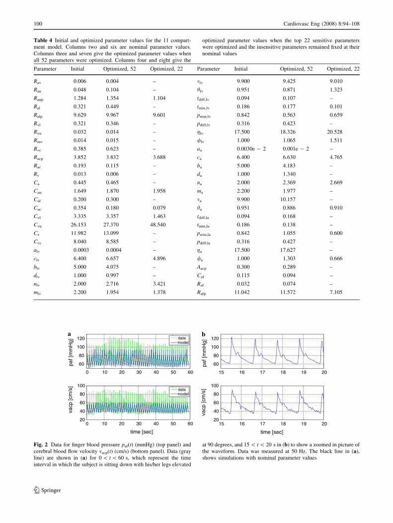
Table 4 Initial and optimized parameter values for the 11 compart-
ment model. Columns two and six are nominal parameter values.
Columns three and seven give the optimized parameter values when
all 52 parameters were optimized. Columns four and eight give the
optimized parameter values when the top 22 sensitive parameters
were optimized and the insensitive parameters remained fixed at their
nominal values
Parameter Initial Optimized, 52 Optimized, 22 Parameter Initial Optimized, 52 Optimized, 22
Rav 0.006 0.004 – mlv 9.900 9.425 9.010
Rau 0.048 0.104 – hlv 0.951 0.871 1.323
Raup 1.284 1.354 1.104 tdiff,lv 0.094 0.107 –
Ral 0.321 0.449 – tmin,lv 0.186 0.177 0.101
Ralp 9.629 9.967 9.601 pmin,lv 0.842 0.563 0.659
Rvl 0.321 0.346 – pdiff,lv 0.316 0.423 –
Rvu 0.032 0.014 – glv 17.500 18.326 20.528
Rmv 0.014 0.015 – /lv 1.000 1.065 1.511
Rvc 0.385 0.623 – aa 0.0030e - 2 0.001e - 2 –
Racp 3.852 3.832 3.688 ca 6.400 6.630 4.765
Rac 0.193 0.115 – ba 5.000 4.183 –
Rv 0.013 0.006 – da 1.000 1.340 –
Ca 0.445 0.465 – na 2.000 2.369 2.669
Cau 1.649 1.870 1.958 ma 2.200 1.977 –
Cal 0.200 0.300 – ma 9.900 10.157 –
Cac 0.354 0.180 0.079 ha 0.951 0.886 0.910
Cvl 3.335 3.357 1.463 tdiff,la 0.094 0.168 –
Cvu 26.153 27.370 48.540 tmin,la 0.186 0.138 –
Cv 11.982 13.099 – pmin,la 0.842 1.055 0.600
Cvc 8.040 8.585 – pdiff,la 0.316 0.427 –
alv 0.0003 0.0004 – ga 17.500 17.627 –
clv 6.400 6.657 4.896 /a 1.000 1.303 0.666
blv 5.000 4.075 – Aacp 0.300 0.289 –
dlv 1.000 0.997 – Caf 0.115 0.094 –
nlv 2.000 2.716 3.421 Raf 0.032 0.074 –
mlv 2.200 1.954 1.378 Rafp 11.042 11.572 7.105
a
0 10 20 30 40 50 60
60
80
100
120
paf [
mm
Hg]
datamodel
0 10 20 30 40 50 6020
40
60
80
100
time [sec]
vacp
[cm
/s]
datamodel
b
15 16 17 18 19 20
60
80
100
120
paf [
mm
Hg]
15 16 17 18 19 2020
40
60
80
100
time [sec]
vacp
[cm
/s]
Fig. 2 Data for finger blood pressure paf(t) (mmHg) (top panel) and
cerebral blood flow velocity vacp(t) (cm/s) (bottom panel). Data (gray
line) are shown in (a) for 0 \ t \ 60 s, which represent the time
interval in which the subject is sitting down with his/her legs elevated
at 90 degrees, and 15 \ t \ 20 s in (b) to show a zoomed in picture of
the waveform. Data was measured at 50 Hz. The black line in (a),
shows simulations with nominal parameter values
100 Cardiovasc Eng (2008) 8:94–108
123

subject. To identify model parameters that characterize a
given time-series dataset we used a weighted least-squares
formulation minimizing the errors between the blood
pressure and blood flow velocity data and the model out-
puts. This weighted least-squares cost functional is given
by
J ¼ 1
N�pdaf
XN
i¼1
pdaf ðtiÞ � pc
af ðtiÞ��� ���2
þ 1
N�vdacp
XN
i¼1
vdacpðtiÞ � vc
acpðtiÞ��� ���2
þ 1
M�pdaf ;sys
XM
i¼1
pdaf ;sysðtiÞ � pc
af ;sysðtiÞ��� ���2
þ 1
M�pdaf ;dia
XM
i¼1
pdaf ;diaðtiÞ � pc
af ;diaðtiÞ��� ���2
þ 1
M�vdacp;sys
XM
i¼1
vdacp;sysðtiÞ � vc
acp;sysðtiÞ��� ���2
þ 1
M�vdacp;dia
XMi¼1
vdacp;diaðtiÞ � vc
acp;diaðtiÞ��� ���2;
where paf is blood pressure in the finger and vacp = qacp/
Aacp is cerebral blood flow velocity, and Aacp represents the
cross-sectional area of the middle cerebral artery. The
subscripts c and d denote computed versus experimental
values, and N is the number of data points in the time-
series. Each term in the functional is weighted by the
average of the data used in that term, denoted by �p and �v:
To get correct representation of the pulse amplitude, spe-
cial emphasis was placed on capturing both peaks and
valleys of the waveform. This is done by including terms
minimizing the difference between systolic and diastolic
values. The time series to be analyzed contains M periods,
thus there will be M systolic and diastolic values.
Since data are only available for two locations, the above
least squares cost functional is not able to ensure correct
physiological ranges for internal states. In particular, we
observed that the model overestimated the baseline aortic
valve resistance defined in (6), which gave rise to an un-
physiologically large discrepancy between the left ventricular
plv,sys systolic pressure and the systolic aortic pressure pa,sys,
Boron and Boulpaep (2003). To avoid the large pressure dis-
crepancy, we added a constraint minimizing the error between
the systolic ventricular pressure and the systolic aortic pres-
sure. Thus an effective cost functional can be written as
J ¼ J þ 1
M�pda;sys
XMi¼1
pca;sysðtiÞ � pc
lv;sysðtiÞ��� ���2: ð8Þ
To identify parameters that minimize the effective cost
functional J we used the Nelder–Mead algorithm Kelley
(1999), which is based on cost functional evaluations on
sequences of simplexes. Optimizations were run using
Matlab 6.5 on a 14-node cluster at Roskilde University,
Denmark, each node with an Intel Pentium 4 2.26 GHz
processor with 1GB RAM. Identification of all 52 param-
eters took 37 h. Simulation results with the model using the
optimized parameters are shown in Fig. 3a and optimized
parameters are listed in Table 4.
Sensitivity Analysis
Results discussed above shows that it is possible to identify
52 parameters. However, due to the large number of
parameters the solution to this optimization problem is not
unique, i.e., a small variation of the nominal parameter
values can lead to large changes in estimates for optimized
parameter values, in particular for parameters that are
insensitive. Thus, to better understand the dependence of
the data on the model parameters, we have analyzed the
sensitivity of the model state variables that represent the
data to each of the parameters. We anticipate that this will
result in a subset of identifiable parameters that when
optimized is able to predict pressure and velocity dynamics
observed in the data.
To derive sensitivity equations for our system of equa-
tions described in (7), we use the basic differential equation
analysis approach described by Eslami (1994) and Frank
(1978). Following this approach we define the relative
sensitivity Sij of the state Xi to parameter lj non-dimen-
sionalized by the state Xi and the parameter value lj as
Sijðt; lÞ��l¼l0¼ oXiðt; lÞ
olj
lj
Xiðt; lÞ
�����l¼l0
; lj;Xiðt; lÞ 6¼ 0:
ð9Þ
Here l0 = [l1,0 … l52,0] denote the nominal values for
the parameters, and we assume all state variables are
continuous. As shown in Fig. 4, Sij(t,l) is a function of
time.
Our goal is to separate model parameters into two
groups, sensitive and insensitive. Therefore, we computed
a maximum relative sensitivity Sj composite over all states
and times for each parameter of the form
Sj ¼ maxi
maxk
Sijðt; lÞ� �����
l¼l0
¼ maxi
maxk
dXiðtk; lÞdlj
lj
Xiðtk; lÞ
!�����l¼l0
: ð10Þ
Because data is only available for the two quantities, finger
pressure paf and cerebral blood flow velocity vacp = qacp/
Aacp, where qacp = (pac - pvc)/Racp, the maximum is
computed over these three states i = paf, pac, and pvc.
Cardiovasc Eng (2008) 8:94–108 101
123

To compute the partial derivatives qXi/qlj, also referred
to as quasi-state variables, each differential equation of the
form (7) is differentiated with respect to each parameter,
assuming that the partial derivatives commute
o
olj
dXi
dt¼ d
dt
oXi
olj
¼ o
olj
FiðX; lÞ: ð11Þ
The sensitivities in (11) are to be solved simultaneously
with the state equations in (7). Together these two systems
of equations result in 11 + 11 9 52 = 583 equations for
the states {pi,Vi} augmented with the quasi-state solutions
qXi/qlj. Thus the full solution is the 11 states and 572
quasi-states.
To get a better understanding for the form of the sen-
sitivity equations, we have derived the equation predicting
the sensitivity Spaf ;Ral; which can be computed by differ-
entiating (2) with respect to Ral,
d
dt
opaf
oRal
� �¼ 1
Caf
1
Raf
opa
oRal
� opaf
oRal
� �� 1
Rafp
opaf
oRal
� opv
oRal
� �� �;
solving for qpaf/qRal, and multiplying by Ral/paf(t). The
resulting solution is shown in Fig. 4, and together with
Table 5 we see that max sensitivity of paf with respect to
Ral is 0.0008. In other words, this parameter is very
insensitive (compare graphs on Fig. 4). The remaining 571
equations can be derived using similar considerations.
However, deriving sensitivity equations using the
analytical approach exemplified above is tedious and
error prone. Alternatively, sensitivities can be derived
using a computational approach, either using finite
differences, which may cause difficulties in multi-scale
problems, or using automatic differentiation (AD), which
uses the chain rule to evaluate derivatives to machine
precision. The latter approach was used to derive
sensitivities for the cardiovascular model. To apply
automatic differentiation, we exploit the chain rule to
rewrite (11) as
o
olj
dXi
dt¼ o
olj
FiðX1; . . .;X11; l1; . . .; l52Þ
¼X11
k¼1
oFi
oXk
oXk
olj
!þ oFi
olj
; ð12Þ
where the Jacobians qF/qX and qF/ql are calculated using
AD, and qX/ql are the quasi-state variables. Thus, the right
hand side of the system of ODE’s in (11) is constructed
with the components of the Jacobians and the quasi-state
variables. Solutions to quasi-state equations give time-
series for dXi/dlj(tk), where k = 1 … N, i represents the
state variables, and j represents each of the 52 parameters.
The above derivation of sensitivity equations required
that the derivatives of the states with respect to each of the
parameters are differentiable. The system of equations
analyzed in this study includes two groups of equations that
a
0 10 20 30 40 50 60
60
80
100
120
paf [
mm
Hg]
DataModel
0 10 20 30 40 50 6020
40
60
80
100
time [sec]
vacp
[cm
/s]
DataModel
b
0 10 20 30 40 50 60
60
80
100
120
paf [
mm
Hg]
DataModel
0 10 20 30 40 50 6020
40
60
80
100
time [sec]
vacp
[cm
/s] Data
Model
Fig. 3 Each panel shows finger pressure paf (top) and cerebral blood
flow velocity vacp (bottom) data and model solutions. (a) Model with
52 parameters optimized, cost of 1.77. (b) Model with the 22 most
sensitive parameters optimized, cost of 1.93
0 2 4 6 8 10 12
−0.5
0
0.5
1
1.5
2
time [sec]
Sen
sitiv
ity o
f paf
cv
Racp
Cal
Ral
Fig. 4 Plots of the relative sensitivity Spaf ;j; where j is parameters cv,
Racp. Cal, and Ral
102 Cardiovasc Eng (2008) 8:94–108
123

do not immediately appear to be fully differentiable: the
three valves in (e.g., (6)) and the heart functions (e.g., (4),
(5)). The valve equations, while piecewise continuous, do
not have derivatives at the cusps between the exponential
function and the constant. To construct a smooth function
that is differentiable, we adapted a smooth approximation,
Chen et al. (2004), of the form
min�ðx1; x2Þ ¼ �� ln
X2
i¼1
e�xi=�
!;
using an � of 0.1. In the heart function, the partial
derivative of the ventricle activation function fi defined
in (5) with respect to the parameter n is given by
of
on¼ ~pn�nm�m bðnÞ
nþ m
� �ð�n�mÞ~tnðbðnÞ
� ~tÞm lnð~tÞ � lnðmÞ � lnbðnÞ
nþ m
� �� �tpv�m
n2
h i;
which is undefined at ~t ¼ 0: However, using L’Hospital’s
Rule, it is possible to determine the limit of this portion of
the equation as ~t! 0: To calculate this limit we let
Kn ¼ ~pn�nm�m bðnÞnþ m
� �ð�n�mÞtpv�m
n2
h i;
yielding
lim~t!0
Kn~tnðb� ~tÞm lnð~tÞ ¼ lim~t!0
Kn1=~t
�n~t�n�1mðb� ~tÞ�m�1¼ 0:
Since f = 0 at b\~t\T ; ofi=on ¼ 0: Thus we have
continuity of qf/qn if we assign qf/qn = 0 at t = 0,
because ~t ¼ T of period i while ~t ¼ 0 of period i + 1. A
similar analysis is done for the remaining partial deriva-
tives with respect to other parameters in the heart
activation function.
Results
Parameter Sensitivity
To rank parameters from the most to the least sensitive,
we solved equations (1) predicting pressures in each of
Table 5 Ranked (most-to-least) sensitivities for 11 compartment model for the pressures pf, pac and pvc with respect to all parameters
Rank Parameter paf pac pvc Sensitivity Rank Parameter paf pac pvc Sensitivity
1 clv 2.029 0.798 0.054 2.029 27 mla 0.139 0.122 0.013 0.139
2 nlv 1.981 1.377 0.043 1.981 28 Ca 0.135 0.076 0.007 0.135
3 hlv 1.270 0.432 0.070 1.270 29 tdiff,lv 0.133 0.039 0.007 0.133
4 Raup 1.084 1.052 0.189 1.084 30 Cv 0.122 0.115 0.074 0.122
5 Ralp 0.401 0.390 0.944 0.944 31 mla 0.092 0.058 0.052 0.092
6 /lv 0.876 0.357 0.022 0.876 32 gla 0.086 0.080 0.008 0.086
7 Cvu 0.874 0.862 0.823 0.874 33 Rvc 0.074 0.065 0.058 0.074
8 Racp 0.679 0.797 0.166 0.797 34 Rau 0.067 0.048 0.003 0.067
9 nla 0.788 0.743 0.122 0.788 35 blv 0.056 0.054 0.005 0.056
10 pmin,lv 0.725 0.279 0.019 0.725 36 Caf 0.051 0.010 0.001 0.051
11 cla 0.668 0.625 0.066 0.668 37 tdiff,la 0.050 0.045 0.005 0.050
12 hla 0.553 0.518 0.049 0.553 38 pdiff,lv 0.049 0.021 0.001 0.049
13 tmin,lv 0.476 0.157 0.026 0.476 39 Rvu 0.042 0.030 0.036 0.042
14 Cvl 0.031 0.030 0.416 0.416 40 bla 0.010 0.008 0.022 0.022
15 Rafp 0.382 0.354 0.005 0.382 41 Raf 0.022 0.001 0.000 0.022
16 mlv 0.378 0.110 0.018 0.378 42 Rmv 0.021 0.020 0.001 0.021
17 /la 0.354 0.296 0.027 0.354 43 pdiff,la 0.020 0.015 0.001 0.020
18 Cau 0.323 0.284 0.048 0.323 44 Rv 0.019 0.017 0.015 0.019
19 mlv 0.288 0.184 0.033 0.288 45 Cal 0.010 0.009 0.003 0.010
20 glv 0.246 0.092 0.007 0.246 46 Rav 0.008 0.003 0.000 0.008
21 pmin,la 0.236 0.220 0.023 0.236 47 Ral 0.008 0.007 0.007 0.008
22 Cac 0.035 0.205 0.005 0.205 48 alv 0.003 0.003 0.000 0.003
23 tmin,la 0.199 0.185 0.020 0.199 49 dlv 0.002 0.001 0.000 0.002
24 Rvl 0.010 0.009 0.173 0.173 50 ala 0.001 0.001 0.002 0.002
25 Rac 0.032 0.163 0.003 0.163 51 dla 0.001 0.000 0.000 0.001
26 Cvc 0.143 0.142 0.110 0.143 52 Aacp 0 0 0 0
Values in boldface are the maximum values for each parameter
Cardiovasc Eng (2008) 8:94–108 103
123
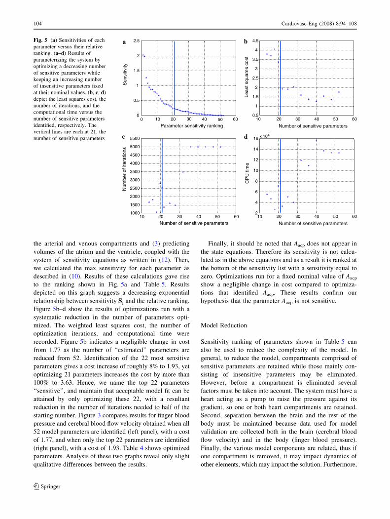
the arterial and venous compartments and (3) predicting
volumes of the atrium and the ventricle, coupled with the
system of sensitivity equations as written in (12). Then,
we calculated the max sensitivity for each parameter as
described in (10). Results of these calculations gave rise
to the ranking shown in Fig. 5a and Table 5. Results
depicted on this graph suggests a decreasing exponential
relationship between sensitivity Sj and the relative ranking.
Figure 5b–d show the results of optimizations run with a
systematic reduction in the number of parameters opti-
mized. The weighted least squares cost, the number of
optimization iterations, and computational time were
recorded. Figure 5b indicates a negligible change in cost
from 1.77 as the number of ‘‘estimated’’ parameters are
reduced from 52. Identification of the 22 most sensitive
parameters gives a cost increase of roughly 8% to 1.93, yet
optimizing 21 parameters increases the cost by more than
100% to 3.63. Hence, we name the top 22 parameters
‘‘sensitive’’, and maintain that acceptable model fit can be
attained by only optimizing these 22, with a resultant
reduction in the number of iterations needed to half of the
starting number. Figure 3 compares results for finger blood
pressure and cerebral blood flow velocity obtained when all
52 model parameters are identified (left panel), with a cost
of 1.77, and when only the top 22 parameters are identified
(right panel), with a cost of 1.93. Table 4 shows optimized
parameters. Analysis of these two graphs reveal only slight
qualitative differences between the results.
Finally, it should be noted that Aacp does not appear in
the state equations. Therefore its sensitivity is not calcu-
lated as in the above equations and as a result it is ranked at
the bottom of the sensitivity list with a sensitivity equal to
zero. Optimizations run for a fixed nominal value of Aacp
show a negligible change in cost compared to optimiza-
tions that identified Aacp. These results confirm our
hypothesis that the parameter Aacp is not sensitive.
Model Reduction
Sensitivity ranking of parameters shown in Table 5 can
also be used to reduce the complexity of the model. In
general, to reduce the model, compartments comprised of
sensitive parameters are retained while those mainly con-
sisting of insensitive parameters may be eliminated.
However, before a compartment is eliminated several
factors must be taken into account. The system must have a
heart acting as a pump to raise the pressure against its
gradient, so one or both heart compartments are retained.
Second, separation between the brain and the rest of the
body must be maintained because data used for model
validation are collected both in the brain (cerebral blood
flow velocity) and in the body (finger blood pressure).
Finally, the various model components are related, thus if
one compartment is removed, it may impact dynamics of
other elements, which may impact the solution. Furthermore,
a
00
0.5
1
1.5
2
2.5
Parameter sensitivity rankingS
ensi
tivity
b
10 20 30 40 50 600.5
1
1.5
2
2.5
3
3.5
4
4.5
Number of sensitive parameters
Leas
t squ
ares
cos
t
c
10 20 30 40 50 60
10 20 30 40 50 60
1000
1500
2000
2500
3000
3500
4000
4500
5000
5500
Number of sensitive parameters
Num
ber
of it
erat
ions
d
10 20 30 40 50 602
4
6
8
10
12
14
16 x 104
Number of sensitive parameters
CP
U ti
me
Fig. 5 (a) Sensitivities of each
parameter versus their relative
ranking. (a–d) Results of
parameterizing the system by
optimizing a decreasing number
of sensitive parameters while
keeping an increasing number
of insensitive parameters fixed
at their nominal values. (b, c, d)
depict the least squares cost, the
number of iterations, and the
computational time versus the
number of sensitive parameters
identified, respectively. The
vertical lines are each at 21, the
number of sensitive parameters
104 Cardiovasc Eng (2008) 8:94–108
123

if the data used for model comparison are not adequate, it
will not be possible to accurately predict the distribution of
blood between compartments. However, instead of
removing a compartment to remove a parameter, it may be
possible to keep one parameter constant, while other
parameters are identified by minimizing the weighted least
squares error between the data and the model.
We first observe that each atrial parameter is signifi-
cantly less sensitive than its corresponding ventricle
parameter. This makes sense physiologically since the
atrium acts primarily as a reservoir and to a lesser extent as
a small priming pump, leaving the primary driver of the
pressure gradient to the ventricle. Therefore the atrium is
removed from the model. We next consider the portion of
the system below the level of the heart. Peripheral resis-
tances Ralp, Raup, and Rafp are all sensitive, as well as
compliances Cvl, Cvu, and Cau. Instead of concluding
immediately that this entire portion of the circulation is
sensitive and therefore necessary to the model, we consider
these results in light of the physiology and the data. Since
we only have data for the brain and the arteries near the
heart, model results obtained for the remainder of the body
are dependent upon each other. In other words, many
combinations of pressures, resistances, and compliances
could comprise the same total resistance and flow in the
body below the heart, leading to the same solution for
arterial blood pressure and cerebral blood flow velocity.
The differentiation between the upper and lower bodies that
was necessary for modeling a data set with standing, i.e.,
gravitational effects, is not necessary with our steady-state
sitting data. Therefore we conclude that sensitive parame-
ters are such because they are dependent upon each other to
provide an effect equal to what would occur with a com-
bined upper and lower body. In addition, note that finger
parameters Caf and Raf are ranked insensitive, at 36 and 41,
respectively. This is likely because the proportion of blood
flowing to the arm is small compared to the rest of the body
and therefore not significant to the model parameterization.
In summary, we eliminated compartments representing
the finger and the left atrium and combined the upper and
lower body compartments. The resulting compartment
model has seven compartments representing the left
ventricle, aorta and vena cava, arteries and veins in the
body as well as in the brain, see Fig. 6. Elimination of the
atrium reduces the number of parameters by 15 (including
Rv); at the same time, elimination of the arterial and
venous compartments reduces the number of parameters
by eight, hence, the proposed reduced model has seven
differential equations and 29 parameters, compared with
11 differential equations and 52 parameters for the full
model. Compared against the full model of with 52
parameters, which had a cost of 1.77, the reduced model
cost is 1.58. Qualitatively the model solution fits the data
similarly in both cases. Equations for this model can be
found in the Appendix.
As we did with the full model, we carried out sensitivity
analysis to rank the parameters with respect to pressures
that represent the data to be studied. For this model these
pressures are: pa, pac, and pvc. Similar to the full model, the
heart parameters are shown to be the most sensitive (n, c, h,
/, tmin, and pmin) though they appear in a slightly different
order. The most sensitive non-heart parameter for this
model is Rasp. This compares well with the full model
where Raup and Ralp showed high sensitivity. Also both the
full model and the reduced model shows high sensitivity to
Racp (ranked 9 and 5 in each, respectively) because it is
explicitly part of one of the equations that directly repre-
sents the data. Finally, it was found from analyses similar
to those done with full model that 20 sensitive parameters
can be accurately estimated in the small model.
vasculature
qmv
Veins Arteries
Heart
Cerebral
Systemic
vasculature
pv
Sys VeinsVvs
Vvc Cer Veins
pvc
Vena cavaVv
Sys Art
Cer Art
pac
Sys Aortapa
qacp
Racp
qac
Rasqas
Rac
Rasp
qasp
qvcRvc
Cac
Cv
Vac
Rav
Left ventricleplv
Clv(t)
Vlv
Ca
Caspvs
Cvspas
Cvc
Rvs qvs
Rmv
Vas
Vaqav
Fig. 6 The 7-compartment
model of systemic circulation,
including arteries (a) and veins
(v) in the brain (cerebral
vasculature, c), the body
(systemic vasculature, s), and
the left ventricle (lv)
Cardiovasc Eng (2008) 8:94–108 105
123

Discussion
In this study we have shown that it is possible to accu-
rately predict 22 of 52 parameters for a single dataset in
our compartment model of systemic blood pressure and
blood flow, while retaining model fit to data as seen in
Fig. 3. Sensitive parameters have physiological signifi-
cance, most of which characterize the left ventricle
waveform or represent lumped peripheral resistances.
Hence, to identify parameter values for multiple datasets
only the most sensitive parameters need to be identified
for each of the datasets, and it would be reasonable to use
literature estimates for the least sensitive parameters and
keep these fixed at nominal values. Based on these pre-
dictions, it would then be possible to calculate means and
standard deviations for each parameter for a given group
of subjects and compare values between different groups
of subjects. We have also shown that it is possible to use
sensitivity information to reduce the proposed model and
design a simpler model that has a similar number of
sensitive parameters. We do not however make any
conclusions on sensitivities during postural change from
sitting to standing. We hypothesize in that case that dif-
ferentiation between upper and lower body due to
gravitational effects would be necessary. Further
investigations include performing the sensitivity analysis
on the previously developed postural change model, O-
lufsen et al. (2005).
Looking specifically at the top 22 parameters of the
original model, it is seen in Table 6 that the majority of the
top sensitive parameters characterize the heart functions,
particularly the ventricle. These parameters are largely
responsible for describing the timing and magnitude of
peak ventricular heart pressure ppv and tpv, respectively.
Because the heart function drives the model, and the peak
pressure and waveform timing in the heart are similar to
that in the aorta and nearby arteries, Boron and Boulpaep
(2003), it is consistent that the model fit would be most
sensitive to these parameters. Not much is known about
these parameters a priori, as opposed to those that are
estimated from known physiological quantities, so finding
parameter values for an individual patient is key for model
parameterization. The peripheral resistances Raup, Ralp,
Racp, and Rafp characterize the largest pressure drops, so it
makes sense that they have a large impact on the solution.
Conversely, we correlate insensitivity of parameters
with known physiology. Each atrial parameter is less sen-
sitive than its corresponding ventricular parameters. This is
consistent with the fact that maximum atrial pressure is
approximately an order of magnitude less than maximum
Table 6 Top 22 sensitive parameters and their effect on the model
Parameter Role in model Effect on model with increase in parameter value
clv Ventricular contractility Increase developed and systolic pressure
nlv Exponent in ventricle polynomial Ventricular peak pressure moves right in time
hlv Median of ventricular tp sigmoid Increase median time for peak pressure at given heart rate
Raup Resistance, upper body arterioles Increase upper body pressure drop
Ralp Resistance, lower body arterioles Increase lower body pressure drop
/lv Median of ventricular pp sigmoid Increase median peak pressure at given heart rate
Cvu Compliance, upper body veins Increase paf and vacp
Racp Resistance, cerebral arterioles Increase cerebral pressure drop
nla Exponent in atrium polynomial Atrial peak pressure moves right in time
pmin,lv Minimum of ventricular pp sigmoid Increase minimum possible peak pressure at given heart rate
cla Atrial contractility Increase developed and systolic pressure
hla Median of atrial tp sigmoid Increase median time for peak pressure at given heart rate
tmin,lv Minimum of tp sigmoid Increase minimum possible peak pressure at given heart rate
Cvl Compliance, lower body veins Increase paf and vacp
Rafp Resistance, finger arterioles Increase finger pressure drop
mlv Steepness of ventricular tp sigmoid Increase distance from median time at given heart rate
/la Median of atrial pp sigmoid Increase median peak pressure at given heart rate
Cau Compliance, upper body arteries Increase paf and vacp, narrow waveforms
mlv Exponent in ventricle polynomial Ventricular peak pressure moves left in time
glv Steepness of ventricular pp sigmoid Increase distance from median time at given heart rate
pmin,la Minimum of atrial pp sigmoid Increase minimum possible peak pressure at given heart rate
Cac Compliance, cerebral arteries Narrow vacp waveform
106 Cardiovasc Eng (2008) 8:94–108
123

ventricular pressure, Boron and Boulpaep (2003), and the
atrium primarily acts as a primer pump. As another
example, the position of dlv representing the volume-
independent component of developed pressure for the
ventricle, is at the bottom of the sensitivity ranking.
Physiologically this could mean several things such as: dlv
could be virtually identical between young adult subjects; it
could be scaled based on the subject but its exact value is
not critical for model fit; or that its place in the model is not
necessary. In immediate future investigations we would
choose to fix parameters such as these at their estimated
from literature values as stated previously and assume that
such values are accurate enough for model fit.
To reach the results in this study we used automatic
differentiation to calculate the gradients used to find the
sensitivities of each parameter with respect to each of the
state variables. While automatic differentiation algorithms
are well-developed and have long been used in languages
such as Fortran, Matlab algorithms are fairly new, Coleman
and Verma (1998) and Forth and Ketzscher (2004). The
main disadvantage of the Matlab algorithms is that they are
slow relative to Fortran and C++. One numerical solve of
the model including sensitivity equations takes about
30 min, and an optimization run with the Nelder–Mead
simplex method not including the sensitivity equations
takes a day and a half. As we wish to analyze multiple
subjects’ data and expand to different populations, speed
will become a necessity. Combining the 30-min-per-itera-
tion automatic differentiation with a many-iteration
optimization routine in Matlab is not reasonable for this
purpose. Therefore we intend to explore automatic differ-
entiation algorithms in Fortran and C++. In addition, using
automatic differentiation for this problem makes it feasible
to investigate the use of gradient-based optimization
methods Kelley (1999), which may lead to more efficient
parameter identification.
Finally, our sensitivity analysis does not tell us anything
about the correlation between parameters. The body is a
closed system of interacting parts, a model of which would
likely contain parameters that act dependently on each
other. Generalized sensitivities, discussed by Thomaseth
and Cobelli (1999), may elucidate interactions between
parameters and also reveal time intervals for which a
parameter is most sensitive. In future work we plan to
investigate the use of this and other sensitivity analysis
methods such as Green’s method, Hwang et al. (1978).
Acknowledgments The authors wish to thank the American Insti-
tute of Mathematics for supporting this work. Authors would like to
acknowledge Dr. Fink, Department of Mathematics, University of
Oxford, UK, who developed the Matlab code for automatic differ-
entiation. The work by M. S. Olufsen and H. T. Tran was supported in
part by NSF-DMS Grant # 0616597. H. T. Tran was supported by
NIH under Grant 9 R01 AI071915-05. C. Zapata was supported in
part by NSA under Grant H98230-06-1-0098 and NSF under Grant
DMS-0552571 as part of the REU summer program. V. Novak,
director of the SAFE Laboratory at BIMDC was supported by NIH-
NIA Harvard Older American Independence Center 2P60 AG08812-
11A1, Core B.
Appendix
Equations, Full Model
(1) Compartment ODE’s:
dpa
dt¼ plvðtÞ�paðtÞ
Rav
�paðtÞ�pauðtÞRau
�paðtÞ�pacðtÞRac
�
�paðtÞ�pafðtÞRaf
�=Ca
dpau
dt¼ paðtÞ�pauðtÞ
Rau
�pauðtÞ�palðtÞRal
�pauðtÞ�pvuðtÞRaup
� �=Cau
dpal
dt¼ pauðtÞ�palðtÞ
Ral
�palðtÞ�pvlðtÞRalp
� �=Cal
dpaf
dt¼ paðtÞ�pafðtÞ
Raf
�pafðtÞ�pvðtÞRafp
� �=Caf
dpac
dt¼ paðtÞ�pacðtÞ
Rac
�pacðtÞ�pvcðtÞRacp
� �=Cac
dpv
dt¼ pvuðtÞ�pvðtÞ
Rvu
þpvcðtÞ�pvðtÞRvc
þpafðtÞ�pvðtÞRafp
�
�pvðtÞ�plaðtÞRv
�=Cv
dpvu
dt¼ pvlðtÞ�pvuðtÞ
Rvl
þpauðtÞ�pvuðtÞRaup
�pvuðtÞ�pvðtÞRvu
� �=Cvu
dpvl
dt¼ palðtÞ�pvlðtÞ
Ralp
�pvlðtÞ�pvuðtÞRvl
� �=Cvl
dpvc
dt¼ pacðtÞ�pvcðtÞ
Racp
�pvcðtÞ�pvðtÞRvc
� �=Cvc
dVlv
dt¼plaðtÞ�plvðtÞ
RmvðtÞ�plvðtÞ�paðtÞ
RavðtÞdVla
dt¼pvðtÞ�plaðtÞ
Rv
�plaðtÞ�plvðtÞRmvðtÞ
Parameters include Ri (mmHg s/cm3), Ci (cm3/mmHg).
2) Valve equations Rav, Rmv, Rvu:
Rav ¼ minðRav;open þ eð�2ðplv�paÞÞ; 20ÞRmv ¼ minðRmv;open þ eð�2ðpla�plvÞÞ; 20ÞRvu ¼ minðRvu;open þ eð�2ðpvu�pvÞÞ; 20Þ
Cardiovasc Eng (2008) 8:94–108 107
123

3) Left atrium and ventricle:
pjðtÞ¼ajðVjðtÞ�bjÞ2þðcjVjðtÞ�djÞfjðtÞ; j¼lv,la
fjðtÞ¼~pjðHÞ
~tnjðbðHÞ�~tÞmjn
nj
j mmj
j ½ðbjðHÞÞ=ðmjþnjÞ�mjþnj0�~t�bjðHÞ
0 bjðHÞ\~t\T
8><>:
~t¼modðt;TÞ
tj¼ðtdiff ;jÞhmj
j
Hmjþhmj
j
þtmin;j
~pj¼ðpdiff ;jÞHgj
Hgjþ/gj
j
þpmin;j
bjðHÞ¼njþmj
njtjðHÞ
Equations, Reduced Model
(1) Compartment ODE’s:
dpa
dt¼ plv � pa
Rav
� pa � pas
Ras
� pa � pac
Rac
� �=Ca
dpv
dt¼ pvs � pv
Rvs
þ pvc � pv
Rvc
� pv � plv
Rmv
� �=Cv
dpas
dt¼ pa � pas
Ras
� pas � pvs
Rasp
� �=Cas
dpvs
dt¼ pas � pvs
Rasp
� pvs � pv
Rvs
� �=Cvs
dpac
dt¼ pa � pac
Rac
� pac � pvc
Racp
� �=Cac
dpvc
dt¼ pac � pvc
Racp
� pvc � pv
Rvc
� �=Cvc
dVlv
dt¼ pv � plv
Rmv
� plv � pa
Rav
(2) Valve equations, Rav, and Rmv:
Rmv ¼ minðRmv;open þ eð�2ðpv�plvÞÞ; 20ÞRav ¼ minðRav;open þ eð�2ðplv�paÞÞ; 20Þ
(3) Left ventricle: Equations for the left ventricle are
identical to those displayed above.
References
Banks H, Bortz D. A parameter sensitivity methodology in the
context of HIV delay equation models. J Math Biol 2005;
50(6):607–25.
Beneken J, DeWit B. A physical approach to hemodynamic aspects of
the human cardiovascular system. In: Reeve E, Guyton A,
editors. Physical bases of circulatory transport: regulation and
exchange. Philadelphia: W.B. Saunders; 1967. p. 1–45.
Bischoff K, Brown R. Drug distribution in mammals. Chem Eng Prog
Symp Ser 1966;50(66):33–45.
Boron W, Boulpaep E. Medical physiology. Philadelphia: Elsevier; 2003.
Bortz B, Nelson P. Sensitivity analysis of nonlinear lumped parameter
models of hiv infection dynamics. J Math Biol 2004;66(5):1009–26.
Carmichael G, Sandu A, Potra F. Sensitivity analysis for atmospheric
chemistry models via automatic differentiation. Atmos Environ
1997;31(3):475–89.
Chen X, Qi L, Teo K-L. Smooth convex approximation to the
maximum eigenvalue function. J Global Opt 2004;30:253–70.
Coleman T, Verma A. ADMAT: an automatic differentiation toolbox
for matlab. Technical report, Computer Science Department,
Cornell University, NY; 1998.
Danielsen M, Ottesen J. Describing the pumping heart as a pressure
source. J Theo Biol 2001;212:71–81.
Ebert T. Sensitivity of fitness to macro-parameter changes: an
analysis of survivorship and individual growth in sea urchin life
histories. Oecologia 1985;65:461–7.
Eslami M. Theory of sensitivity in dynamic systems: an introduction.
Berlin: Springer-Verlag; 1994.
Forth S, Ketzscher R. High-level interfaces for the MAD (Matlab
Automatic Differentiation) package. In: Neittaanmaki P, et al.
editors. ECCOMAS 2004: fourth European congress on compu-
tational methods in applied sciences and engineering. European
Community on Computational Methods in Applied Sciences; 2004.
Frank P. Introduction to sensitivity theory. New York: Academic
Press; 1978.
Heldt T, Shim E, Kamm R, Mark R. Computational modeling of
cardiovascular response to orthostatic stress. J Appl Physiol 2002;
92(3):1239–54.
Hwang J-T, Dougherty E, Rabitz S, Rabitz H. The Green’s function
method of sensitivity analysis in chemical kinetics. J Chem Phys
1978;69(11):5180–91.
Kappel F, Peer R. A mathematical model for fundamental regulation
processes in the cardiovascular system. J Math Biol
1993;31(6):611–31.
Kelley C. Iterative methods for optimization. Philadelphia: Society
for Industrial and Applied Mathematics; 1999.
Middleman S. Transport phenomena in the circulatory system. New
York: Wiley-Interscience; 1972.
Nadler S, Hidalgo J, Bloch T. Prediction of blood volume in normal
human adults. Surgery. 1962;51:224–32.
Novak V, Hu K, Vyas M, Lipsitz L. Cardiolocomotor coupling in
young and elderly people. J Gerontol A Biol Sci Med Sci 2007;
62(1):86–92.
Olufsen M, Tran H, Ottesen J. Modeling cerebral blood flow control
during posture change from sitting to standing. J Cardiovasc Eng
2004;4(1):47–58.
Olufsen M, Tran H, Ottesen J, Ellwein L, Lipsitz L, Novak V. Blood
pressure and blood flow variation during postural change from
sitting to standing – modeling and experimental validation. J
Appl Physiol 2005;99(4):1523–37.
Olufsen M, Tran H, Ottesen J, Lipsitz L, Novak V. Modeling
baroreflex regulation of heart rate during orthostatic stress. Am J
Physiol 2006;291:R1355–68.
Ottesen J. Modeling of the baroreflex-feedback mechanism with time-
delay. J Math Biol 1997a;36:41–63.
Ottesen J. Nonlinearity of baroreceptor nerves. Surv Math Ind
1997b;7:187–201.
Ottesen J, Danielsen M. Modeling ventricular contraction with heart
rate changes. J Theo Biol 2003;222(3):337–46.
Rabitz H, Kramer M, Dacol D. Sensitivity analysis in chemical
kinetics. Ann Rev Phys Chem 1983;34:419–61.
Rideout V. Mathematical and computer modeling of physiological
systems. New Jersey: Prentice Hall; 1991.
Thomaseth K, Cobelli C. Generalized sensitivity functions in
physiological identification. Ann Biomed Eng 1999;27:607–16.
Ursino M. Interaction between carotid baroregulation and the
pulsating heart: a mathematical model. Am J Physiol 1998;44:
H1733–47.
108 Cardiovasc Eng (2008) 8:94–108
123