Sensitivity Analysis for Calibrating VISSIM in Modeling the Zurich Network

Qiao Ge & Monica Menendez Traffic Engineering Group (SVT)

ETH Zurich IVT

02.05.2012

12th Swiss Transport Research Conference (Ascona)

• Project: Calibration Study for VISSIM (CSV)

• Study area: inner city of Zurich (around 2.6 km2)

• Simulation period: 1-hour in the evening peak (17:00 to 18:00)

• Scope of work: optimize the calibration process, so the City of Zurich could calibrate the VISSIM model in the most efficient way, tailored to its specific needs and requirements.

Background

2

Study Area of CSV

Source: City of Zurich, 2011 3

4

Challenges of the Calibration Process

Many param-eters

Public transport

Hills

• Computational cost is very high (> 20 min per simulation run) • The brute-force approach is not feasible for the calibration

5

Pre-selection of Parameters (1/2)

Each parameter was analyzed individually, and categorized according to its relevance within the Zurich model

6

Pre-selection of Parameters (2/2)

192 total VISSIM parameters

148 relevant

14 SA

Parameters

Introduction of EE Method

The method we developed is based on the Elementary

Effects (EE) method:

Qualitative and stochastic approach

Efficient approach to analyze complex models

It has been applied with e.g. chemistry and

environmental engineering models, but never with a

microscopic traffic model

7

Definition of Elementary Effect

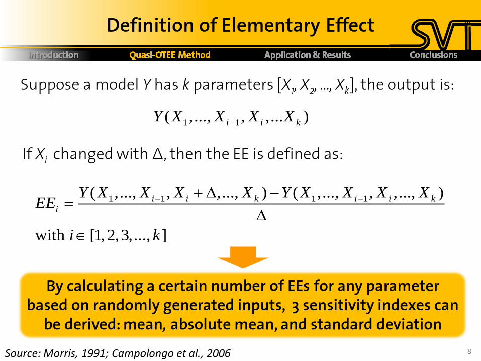
Suppose a model Y has k parameters [X1, X2, …, Xk], the output is:

8

1 1 1 1( ,..., , ,..., ) ( ,..., , ,..., )

with [1,2,3,..., ]

i i k i i k

i

Y X X X X Y X X X XEE

i k

If Xi changed with Δ, then the EE is defined as:

1 1( ,..., , ,... )i i kY X X X X

Source: Morris, 1991; Campolongo et al., 2006

By calculating a certain number of EEs for any parameter based on randomly generated inputs, 3 sensitivity indexes can

be derived: mean, absolute mean, and standard deviation

Sampling Strategy (1/2)

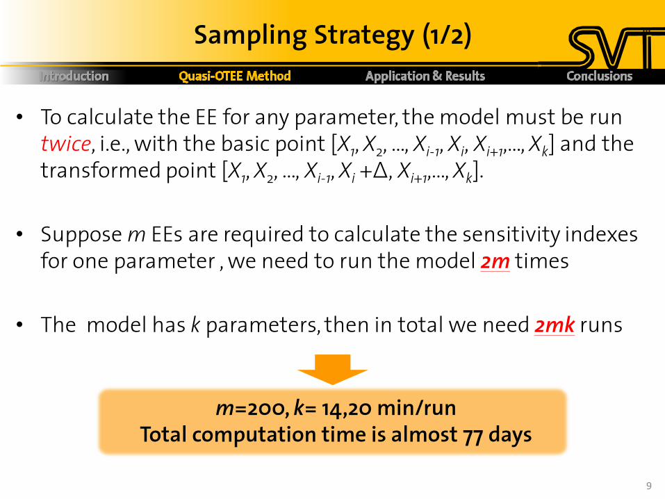
• To calculate the EE for any parameter, the model must be run twice, i.e., with the basic point [X1, X2, …, Xi-1, Xi, Xi+1,…, Xk] and the transformed point [X1, X2, …, Xi-1, Xi +Δ, Xi+1,…, Xk].

• Suppose m EEs are required to calculate the sensitivity indexes for one parameter , we need to run the model 2m times

• The model has k parameters, then in total we need 2mk runs

9

m=200, k= 14,20 min/run Total computation time is almost 77 days

X2

X1

Δ

Δ

X10

X20

X1 X2

P0 X10 X2

0

P1 X10 + Δ X2

0

P2 X10 + Δ X2

0 + Δ

Sampling Strategy (2/2)

10

EE(X1) = [Y(P1) - Y(P0)] / Δ k+1 points

k+1 points = one trajectory

EE(X2) = [Y(P2) - Y(P1)] / Δ P0 P1

P2

A model with 2 parameters [X1 , X2]

m=200, k= 14, 20 min/run Total computation time is almost 41 days

If randomly sampling m trajectories, we will get the same amount of EE, but only need m(k+1) runs.

Optimized Trajectories (1/2)

Solution:

Reduce the total number of trajectories, but keep as many sample

points as possible.

11 Source: Campolongo et al., 2006

Find an optimized set of trajectories that covers as much as possible the total input space

Optimized Trajectories (2/2)

1. Randomly generate m (e.g. m = 200) trajectories

2. Calculate the Euclidean distance between any 2 trajectories

3. Enumerate all possible sets containing n trajectories from those m random

trajectories (n<<m)

4. Compute the total distance D for each trajectory set

5. The set with the longest D is the OT set

12 Source: Campolongo et al., 2006 12

n =10, k = 14, 20 min/run Total computation time for EE is about 2 days

Problem of the Original OT Approach

However:

When m is a large number, the total number of possible trajectory

sets N (= 𝑚!

𝑛!∗ 𝑚−𝑛 !) could be enormous:

13

m = 200, n = 10, N ≈ 2 x 1016 Total computation time for enumerating is around 50 days

Quasi-Optimized Trajectories

Step 1: Pick the set (named S1) of m – 1 trajectories that have the longest Euclidean

distance from the original set of m trajectories (named S0)

Step 2: Pick the set (named S2) of m – 2 trajectories which have the maximum dispersion

based on S1

……

Step m-n: only n trajectories have been left

Total combinations = 𝑚 + 𝑚− 1 +⋯+ 𝑛 =𝑚+𝑛 𝑚−𝑛+1

2≪

𝑚!

𝑛!∗ 𝑚−𝑛 ! .

Although the result may not always be identical to the one obtained with the original OT approach, it is a good compromise between accuracy and efficiency.

14

n=10, m= 200, N=20055 Total computation time is about 15 minutes

Review of Process

15

77 days

41 days

2 + 50 days

2 days

Basic EE method

EE + use of trajectories as a sampling strategy

EE + original OT Approach

Quasi-OTEE Method

Software Development for SA

16

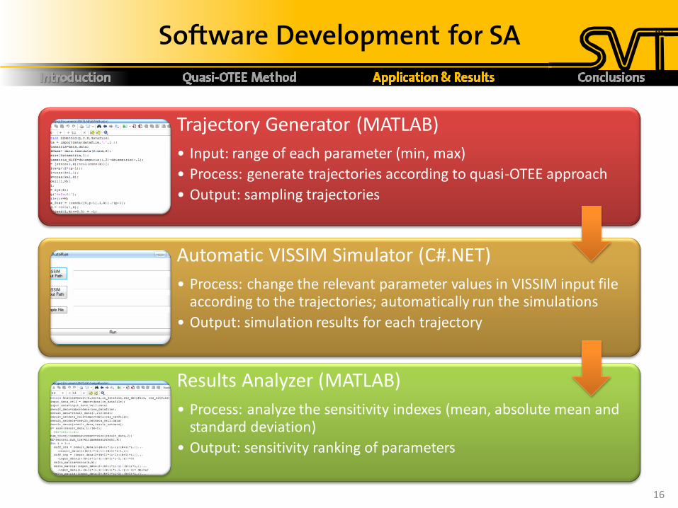
Trajectory Generator (MATLAB)

• Input: range of each parameter (min, max)

• Process: generate trajectories according to quasi-OTEE approach

• Output: sampling trajectories

Automatic VISSIM Simulator (C#.NET)

• Process: change the relevant parameter values in VISSIM input file according to the trajectories; automatically run the simulations

• Output: simulation results for each trajectory

Results Analyzer (MATLAB)

• Process: analyze the sensitivity indexes (mean, absolute mean and standard deviation)

• Output: sensitivity ranking of parameters

Travel Time Measurement in VISSIM

8 travel time measurement sections

17

1

2

3 7

6

8

4

5

High Through Flow (≈ 300 veh/h): 4, 5 and 8 Mid Through Flow (≈100 veh/h): 1 and 2 Low Through Flow (<20 veh/h): 3, 6 and 7

SA Results (1/2)

18

0

0.1

0.2

0.3

0.4

0.5

0.6

0.7

0.8

0.9

1

Sensitivity Ranking of Parameters

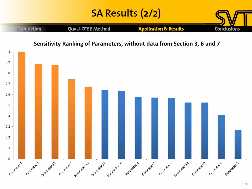
SA Results (2/2)

19

0

0.1

0.2

0.3

0.4

0.5

0.6

0.7

0.8

0.9

1

Sensitivity Ranking of Parameters, without data from Section 3, 6 and 7

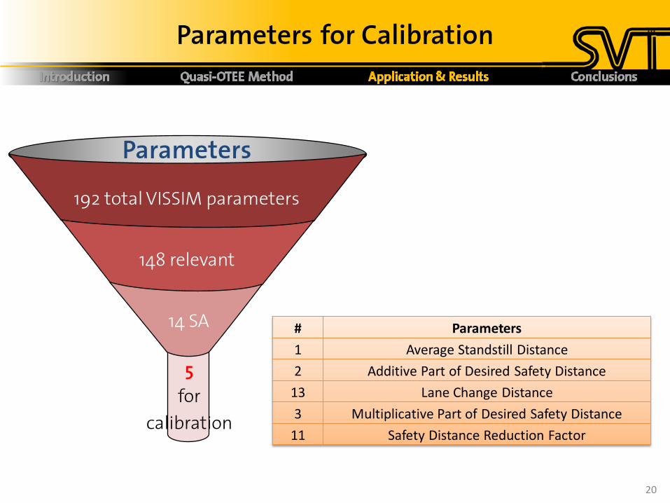
Parameters for Calibration

20

192 total VISSIM parameters

148 relevant

14 SA

Parameters

5

for

calibration

# Parameters

1 Average Standstill Distance

2 Additive Part of Desired Safety Distance

13 Lane Change Distance

3 Multiplicative Part of Desired Safety Distance

11 Safety Distance Reduction Factor

Conclusions

• The quasi-OTEE method is an improvement to the EE method

• It is efficient to deal with the SA for VISSIM: e.g., the time cost of

SA in the CSV project was reduced from 77 days to 2 days

• It is able to identify the most important parameters of a

complex model in an accurate way

Potential extensions:

• Optimize the sampling process

• Validate the method under many different scenarios

21