sensitivity analysis for functional structural plant modelling
TRANSCRIPT

HAL Id: tel-00719935https://tel.archives-ouvertes.fr/tel-00719935
Submitted on 2 Jul 2014
HAL is a multi-disciplinary open accessarchive for the deposit and dissemination of sci-entific research documents, whether they are pub-lished or not. The documents may come fromteaching and research institutions in France orabroad, or from public or private research centers.
L’archive ouverte pluridisciplinaire HAL, estdestinée au dépôt et à la diffusion de documentsscientifiques de niveau recherche, publiés ou non,émanant des établissements d’enseignement et derecherche français ou étrangers, des laboratoirespublics ou privés.
Sensitivity Analysis for Functional Structural PlantModellingQiongli Wu
To cite this version:Qiongli Wu. Sensitivity Analysis for Functional Structural Plant Modelling. Other. Ecole CentraleParis, 2012. English. NNT : 2012ECAP0021. tel-00719935

ECOLE CENTRALE DES ARTS
ET MANUFACTURES“ECOLE CENTRALE PARIS”
Dissertationpresented by: Qiongli WU
for the degree of Doctor of Applied Mathematics
Speciality: Applied MathematicsLaboratory: Mathematiques Appliquees aux Systemes (MAS)
Sensitivity Analysis for Functional Structural PlantModelling
Date of defense :19/04/2012Composition of jury:
M. Stefano TARANTOLA (President, Reviewer)M. Gerhard BUCK-SORLIN (Reviewer)M. Enrico ZIOMs. Amelie MATHIEU
M. Paul-Henry COURNEDE (Supervisor)
N ordre : 2012ECAP0021


Sensitivity Analysis for Functional Structural PlantModelling
Global sensitivity analysis has a key role to play in the design and parameterizationof functional-structural plant growth models (FSPM) which combine the descriptionof plant structural development (organogenesis and geometry) and functional growth(biomass accumulation and allocation). Models of this type generally describe manyinteracting processes, count a large number of parameters, and their computationalcost can be important. The general objective of this thesis is to develop a propermethodology for the sensitivity analysis of functional structural plant models and toinvestigate how sensitivity analysis can help for the design and parameterization ofsuch models as well as providing insights for the understanding of underlying biologicalprocesses. Our contribution can be summarized in two parts: from the methodologypoint of view, we first improved the performance of the existing Sobol’s method tocompute sensitivity indices in terms of computational efficiency, with a better controlof the estimation error for Monte Carlo simulation, and we also designed a properstrategy of analysis for complex biophysical systems; from the application point ofview, we implemented our strategy for 3 FSPMs with different levels of complexity,and analyzed the results from different perspectives (model parameterization, modeldiagnosis).
Keywords: Sensitivity analysis, FSPM, SRC, Sobol’s method, Non-linearity assess-ment, Error estimation, GreenLab, NEMA


Analyse de Sensibilite pour la ModelisationStructure-Fonction des Plantes
L’analyse de sensibilite globale a un role cle a jouer dans la conception et la pa-rametrisation des modeles structure-fonction de la croissance des plantes (FSPM).Ceux-ci combinent la description du developpement structurel des plantes (organoge-nese et geometrie) et de leur croissance fonctionnelle (accumulation de biomasse etallocation). Les modeles de ce type decrivent generalement de nombreux processus eninteraction, comptent un grand nombre de parametres et leur cout de calcul peut etreimportant. L’objectif de cette these est de developper une methodologie approprieepour l’analyse de sensibilite des modeles structure-fonction des plantes et d’etudiercomment l’analyse de sensibilite peut aider a la conception et la parametrisation deces modeles, ainsi qu’a l’analyse et la comprehension des processus biologiques en jeu.Notre contribution peut etre vue en deux parties : du point de vue methodologiqueet du point de vue de l’application des methodes aux modeles. D’un point de vuemethodologique, nous avons tout d’abord ameliore les performances de la methode deSobol pour le calcul des indices de sensibilite en termes d’efficacite de calcul, avec unmeilleur controle de l’erreur d’estimation par les simulations de Monte Carlo. Nousavons egalement concu une strategie d’analyse adaptee aux systemes biophysiquescomplexes. Du point de vue applicatif, nous avons implemente notre strategie pour 3FSPMs avec des niveaux de complexite differents, et nous avons analyse les resultatsselon differents aspects, parametrisation et diagnostic de modeles.
Mots-cles : Analyse de sensibilite, FSPM, SRC, Sobol, Indice de linearite, Estima-tion de l’erreur, GreenLab, NEMA


CONTENTS
Liste of figures . . . . . . . . . . . . . . . . . . . . . . . . . . . . . . . . . . . . 11
Liste of tables . . . . . . . . . . . . . . . . . . . . . . . . . . . . . . . . . . . . 13
1. Introduction . . . . . . . . . . . . . . . . . . . . . . . . . . . . . . . . . . . 15
1.1 General background . . . . . . . . . . . . . . . . . . . . . . . . . . . . . 15
1.2 Important issues in SA of FSPMs . . . . . . . . . . . . . . . . . . . . . 21
1.3 Objectives of this work . . . . . . . . . . . . . . . . . . . . . . . . . . . 24
1.4 Organization of the dissertation . . . . . . . . . . . . . . . . . . . . . . 25
Part I Preliminaries 27
2. FSPM . . . . . . . . . . . . . . . . . . . . . . . . . . . . . . . . . . . . . . . 29
2.1 General concepts about FSPM . . . . . . . . . . . . . . . . . . . . . . . 29
2.2 Functional-structural plant model design steps . . . . . . . . . . . . . . 31
2.3 Limitations and challenges of FSPMs . . . . . . . . . . . . . . . . . . . 34
2.4 Introduction to several FSPMs . . . . . . . . . . . . . . . . . . . . . . . 35
2.4.1 GreenLab model for maize . . . . . . . . . . . . . . . . . . . . . 35
2.4.2 GreenLab model for poplar tree . . . . . . . . . . . . . . . . . . 37
2.4.3 NEMA model for wheat . . . . . . . . . . . . . . . . . . . . . . 40
2.5 Concluding remarks . . . . . . . . . . . . . . . . . . . . . . . . . . . . . 41
3. Sensitivity analysis for FSPM . . . . . . . . . . . . . . . . . . . . . . . . . 45
3.1 Uncertainty analysis and sensitivity analysis . . . . . . . . . . . . . . . 45
3.2 Model definition . . . . . . . . . . . . . . . . . . . . . . . . . . . . . . . 46
3.3 Model inputs . . . . . . . . . . . . . . . . . . . . . . . . . . . . . . . . 47
3.4 Purpose of sensitivity analysis . . . . . . . . . . . . . . . . . . . . . . . 48
3.5 SA methods . . . . . . . . . . . . . . . . . . . . . . . . . . . . . . . . . 50
3.5.1 Classification of methods . . . . . . . . . . . . . . . . . . . . . . 50
3.5.2 Description of methods . . . . . . . . . . . . . . . . . . . . . . . 51
3.6 Basic steps of SA for FSPM . . . . . . . . . . . . . . . . . . . . . . . . 56
3.7 Concluding remarks . . . . . . . . . . . . . . . . . . . . . . . . . . . . . 58

8 Contents
Part II Algorithm and methodology design 59
4. An Efficient Computational Method for Global Sensitivity Analysis . . . 61
4.1 Computation of sensitivity indices . . . . . . . . . . . . . . . . . . . . . 61
4.1.1 General concepts of Sobol’s sensitivity analysis . . . . . . . . . . 61
4.1.2 Sobol’s computing method and H-S improvement . . . . . . . . 63
4.1.3 A new method to compute Sobol’s indices . . . . . . . . . . . . 65
4.2 Error estimation for Sobol’s method . . . . . . . . . . . . . . . . . . . . 68
4.2.1 Standard error, probable error . . . . . . . . . . . . . . . . . . . 68
4.2.2 For Sobol’s formula . . . . . . . . . . . . . . . . . . . . . . . . . 69
Error estimation for Si . . . . . . . . . . . . . . . . . . . . . . . 70
error estimation for STi . . . . . . . . . . . . . . . . . . . . . . 72
4.3 Computational Tests . . . . . . . . . . . . . . . . . . . . . . . . . . . . 72
4.3.1 Analytical functions . . . . . . . . . . . . . . . . . . . . . . . . 72
4.3.2 error estimation test . . . . . . . . . . . . . . . . . . . . . . . . 73
4.3.3 Comparison of H-S and proposed method . . . . . . . . . . . . . 73
4.4 Discussion . . . . . . . . . . . . . . . . . . . . . . . . . . . . . . . . . . 74
5. Strategy design . . . . . . . . . . . . . . . . . . . . . . . . . . . . . . . . . 77
5.1 Introduction . . . . . . . . . . . . . . . . . . . . . . . . . . . . . . . . . 77
5.2 SRC method and non-linearity assessment . . . . . . . . . . . . . . . . 79
5.3 A methodology for complex biophysical models . . . . . . . . . . . . . 82
5.4 Processing for functional output case . . . . . . . . . . . . . . . . . . . 88
5.5 Concluding remarks and discussions . . . . . . . . . . . . . . . . . . . . 91
6. Software platform: PyGMAlion . . . . . . . . . . . . . . . . . . . . . . . . 93
6.1 Background and objectives . . . . . . . . . . . . . . . . . . . . . . . . . 93
6.2 PyGMAlion . . . . . . . . . . . . . . . . . . . . . . . . . . . . . . . . . 94
6.3 Implementation in PyGMAlion . . . . . . . . . . . . . . . . . . . . . . 95
6.4 Sensitivity analysis in PyGMAlion . . . . . . . . . . . . . . . . . . . . . 98
Part III Applications and simulations 101
7. Methodology practice: application to FSPMs . . . . . . . . . . . . . . . . 103
7.1 GreenLab maize . . . . . . . . . . . . . . . . . . . . . . . . . . . . . . . 103
7.1.1 Local sensitivity analysis and its normalized version . . . . . . . 103
7.1.2 Standardized Regression coefficients . . . . . . . . . . . . . . . . 105
7.1.3 Sobol’s method . . . . . . . . . . . . . . . . . . . . . . . . . . . 107
7.1.4 Discussion . . . . . . . . . . . . . . . . . . . . . . . . . . . . . . 111
7.2 Poplar tree model . . . . . . . . . . . . . . . . . . . . . . . . . . . . . . 112
7.3 Model of C-N dynamics (NEMA) . . . . . . . . . . . . . . . . . . . . . 115
7.3.1 Output AreaGreenTotal . . . . . . . . . . . . . . . . . . . . . . 116

Contents 9
7.3.2 Output Production . . . . . . . . . . . . . . . . . . . . . . . . . 127
7.3.3 Output DMgrains . . . . . . . . . . . . . . . . . . . . . . . . . . 132
7.3.4 Output Ngrains . . . . . . . . . . . . . . . . . . . . . . . . . . . 135
7.3.5 Output RootNuptake . . . . . . . . . . . . . . . . . . . . . . . . 140
7.3.6 Comprehensive comparison . . . . . . . . . . . . . . . . . . . . . 145
7.4 Conclusions and discussion . . . . . . . . . . . . . . . . . . . . . . . . . 147
Part IV Conclusions and perspectives 149
8. Conclusions and perspectives . . . . . . . . . . . . . . . . . . . . . . . . . 151
8.1 Contributions . . . . . . . . . . . . . . . . . . . . . . . . . . . . . . . . 151
8.2 Discussion and perspectives . . . . . . . . . . . . . . . . . . . . . . . . 157
8.3 To conclude . . . . . . . . . . . . . . . . . . . . . . . . . . . . . . . . . 160
Appendix 163
A. Approximation of the moments of functions of random variables . . . . . 165
Bibliography . . . . . . . . . . . . . . . . . . . . . . . . . . . . . . . . . . . . . 169
Acknowledgment . . . . . . . . . . . . . . . . . . . . . . . . . . . . . . . . . . 179
Publications . . . . . . . . . . . . . . . . . . . . . . . . . . . . . . . . . . . . . 181

10 Contents

LIST OF FIGURES
1.1 Methodology: Sketch of the various SA techniques available . . . . . . 22
2.1 Poplar tree: topology after 30 time steps . . . . . . . . . . . . . . . . . 38
2.2 NEMA: Overview scheme . . . . . . . . . . . . . . . . . . . . . . . . . 42
5.1 Non-linearity assessment: GreenLab Maize . . . . . . . . . . . . . . . . 80
5.2 Non-linearity assessment: Poplar tree . . . . . . . . . . . . . . . . . . . 81
5.3 Non-linearity assessment: NEMA . . . . . . . . . . . . . . . . . . . . . 81
5.4 Methodology: Mesh grid 3 dimension parameter space . . . . . . . . . 84
5.5 Methodology: ST gΩi
for one module decomposition scheme . . . . . . . 88
5.6 Methodology: Si for 35 parameters . . . . . . . . . . . . . . . . . . . . 89
5.7 Methodology: Total variance of output . . . . . . . . . . . . . . . . . . 90
6.1 PyGMAlion: Sensitivity analysis configuration . . . . . . . . . . . . . . 99
7.1 GreenLab Maize: Biomass allocation at each GC . . . . . . . . . . . . 104
7.2 GreenLab maize: Local sensitivity analysis . . . . . . . . . . . . . . . . 105
7.3 GreenLab maize: SRCs for the outputs q . . . . . . . . . . . . . . . . . 107
7.4 GreenLab maize:∑
(γXi)2 and R2
Y . . . . . . . . . . . . . . . . . . . . 107
7.5 GreenLab maize: Si and STi for µ . . . . . . . . . . . . . . . . . . . . . 108
7.6 GreenLab maize: linearity indexes, Sp and µ fixed . . . . . . . . . . . . 109
7.7 GreenLab maize: Sobol’s method for SA, Sp and µ fixed . . . . . . . . 110
7.8 GreenLab maize: STi and Si for αb . . . . . . . . . . . . . . . . . . . . 110
7.9 GreenLab maize: Interactions between αb to the other parameters . . . 111
7.10 Poplar tree: Oscillation of Q/D . . . . . . . . . . . . . . . . . . . . . . 112
7.11 Poplar tree: Number of phytomers of physiological age 4 . . . . . . . . 113
7.12 Poplar tree: Evolution of linearity index . . . . . . . . . . . . . . . . . 113
7.13 Poplar tree: Sensitivity indexes for all the model parameters . . . . . . 114
7.14 Poplar tree: Sensitivity indices when fixing µ and Sp . . . . . . . . . . 115
7.15 NEMA: Output AreaGreenTotal, Linearity . . . . . . . . . . . . . . . . 117
7.16 NEMA: Output AreaGreenTotal, SgΩi
. . . . . . . . . . . . . . . . . . . 118
7.17 NEMA: Output AreaGreenTotal, ST gΩi
− SgΩi
. . . . . . . . . . . . . . . 119
7.18 NEMA: Output AreaGreenTotal, SgΩij
. . . . . . . . . . . . . . . . . . . 119
7.19 NEMA: Output AreaGreenTotal, Selected factors Si . . . . . . . . . . . 124
7.20 NEMA: Output AreaGreenTotal, Selected factors STi − Si . . . . . . . 126

12 List of Figures
7.21 NEMA: Output Production, Linearity . . . . . . . . . . . . . . . . . . 128
7.22 NEMA: Output Production, SgΩi
. . . . . . . . . . . . . . . . . . . . . . 128
7.23 NEMA: Output Production, ST gΩi
− SgΩi
. . . . . . . . . . . . . . . . . 129
7.24 NEMA: Output Production, SgΩij
. . . . . . . . . . . . . . . . . . . . . 129
7.25 NEMA: Output Production, Selected factors Si . . . . . . . . . . . . . 130
7.26 NEMA: Output Production, Selected factors STi − Si . . . . . . . . . . 131
7.27 NEMA: Output DMgrains, Linearity . . . . . . . . . . . . . . . . . . . 132
7.28 NEMA: Output DMgrains, SgΩi
. . . . . . . . . . . . . . . . . . . . . . 133
7.29 NEMA: Output DMgrains, Selected factors Si . . . . . . . . . . . . . . 134
7.30 NEMA: Output Ngrains, Linearity . . . . . . . . . . . . . . . . . . . . 135
7.31 NEMA: Output Ngrains, SgΩi
. . . . . . . . . . . . . . . . . . . . . . . . 136
7.32 NEMA: Output Ngrains, ST gΩi
− SgΩi
. . . . . . . . . . . . . . . . . . . 136
7.33 NEMA: Output Ngrains, SgΩij
. . . . . . . . . . . . . . . . . . . . . . . 137
7.34 NEMA: Output Ngrains, Selected factors Si . . . . . . . . . . . . . . . 138
7.35 NEMA: Output Ngrains, Selected factors STi − Si . . . . . . . . . . . . 139
7.36 NEMA: Output RootNuptake, Linearity . . . . . . . . . . . . . . . . . 140
7.37 NEMA: Output RootNuptake, SgΩi
. . . . . . . . . . . . . . . . . . . . 141
7.38 NEMA: Output RootNuptake, ST gΩi
− SgΩi
. . . . . . . . . . . . . . . . 141
7.39 NEMA: Output RootNuptake, SgΩij
. . . . . . . . . . . . . . . . . . . . 142
7.40 NEMA: Output RootNuptake, Selected factors Si . . . . . . . . . . . . 143
7.41 NEMA: Output RootNuptake, Selected factors STi − Si . . . . . . . . . 144
8.1 Brief illustration of improved Sobol’s estimator. . . . . . . . . . . . . . 152

LIST OF TABLES
2.1 GreenLab Maize: Parameter Distributions . . . . . . . . . . . . . . . . 37
2.2 GreenLab poplar tree: Parameter Distributions . . . . . . . . . . . . . 40
2.3 NEMA: Model parameters . . . . . . . . . . . . . . . . . . . . . . . . . 43
4.1 Sobol’s Estimator improvement . . . . . . . . . . . . . . . . . . . . . . 66
4.2 H-S Sobol’s method for Si . . . . . . . . . . . . . . . . . . . . . . . . . 74
4.3 H-S Sobol’s method for STi . . . . . . . . . . . . . . . . . . . . . . . . 75
4.4 Efficiency comparison of H-S and new Sobol’s method for Si . . . . . . 75
4.5 Efficiency comparison of H-S and new Sobol’s method for STi . . . . . 76
7.1 GreenLab maize: SRC index and R2 at selected typical GC . . . . . . . 106
7.2 NEMA: List of tables and figure describing the results of SA . . . . . . 116
7.3 NEMA: Output AreaGreenTotal, Module DMfluxes . . . . . . . . . . . 120
7.4 NEMA: Output AreaGreenTotal, Module Nfluxes . . . . . . . . . . . . 121
7.5 NEMA: Output AreaGreenTotal, Module Photosynthesis . . . . . . . . 121
7.6 NEMA: Output AreaGreenTotal, Module RootNuptake . . . . . . . . . 122
7.7 NEMA: Output AreaGreenTotal, Module Tissuedeath . . . . . . . . . . 122
7.8 NEMA: Output AreaGreenTotal, Overall parameter selection analysis . 122
7.9 NEMA: Output AreaGreenTotal, Intra-Module Interaction analysis . . 123
7.10 NEMA: Output AreaGreenTotal, Inter-Module Interaction . . . . . . . 123
7.11 NEMA: Output AreaGreenTotal, Sij for selected factors . . . . . . . . 125
7.12 NEMA: Output Production, Selected factors list . . . . . . . . . . . . . 130
7.13 NEMA: Output Production, Overall parameter selection analysis . . . . 130
7.14 NEMA: Output DMgrains, Selected factors . . . . . . . . . . . . . . . . 133
7.15 NEMA: Output DMgrains, Overall parameter selection analysis . . . . 133
7.16 NEMA: Output Ngrains, Selected factors . . . . . . . . . . . . . . . . . 137
7.17 NEMA: Output Ngrains, Overall parameter selection analysis . . . . . 137
7.18 NEMA: Output Ngrains, Intra-Module Interaction analysis . . . . . . . 137
7.19 NEMA: Output Ngrains, Inter-Module Interaction . . . . . . . . . . . . 138
7.20 NEMA: Output Ngrains, Sij at thermal time after flowering 685.063 Cd 138
7.21 NEMA: Output RootNuptake, Selected factors . . . . . . . . . . . . . . 142
7.22 NEMA: Output RootNuptake, Overall parameter selection analysis . . 142
7.23 NEMA: Output RootNuptake, Intra-Module Interaction analysis . . . . 143
7.24 NEMA: Output RootNuptake, Inter-Module Interaction . . . . . . . . . 143
7.25 NEMA: Selected Si ranking in overall model for different outputs . . . 146

14 List of Tables

1. INTRODUCTION
1.1 General background
Mathematical modelling
Mathematical modelling is a key tool for the analysis of a wide range of real-worldphenomena ranging from physics and engineering to chemistry, biology and economics[Weiβe, 2009]. A mathematical model is defined by a series of equations, input factors,parameters, and state variables to characterize the processes being investigated. Anincreasing number of models have been developed in recent decades thanks to theprogress of computational and statistical tools.
The purposes of modelling include: 1) integration of knowledge (exceeding thecapacity of the human brain), 2) quantitative testing of hypotheses, 3) extrapolationof effects of factors beyond the range of conditions covered experimentally, 4) revealingof knowledge gaps and ‘guiding’ research, and 5) support of practical managementdecisions. In research environments, modelling commonly serves purposes such asintegrating knowledge or the quantitative testing of hypotheses [Vos et al., 2007].Through a better understanding of phenomena and the prediction and simulation ofthe impact of decisions, the different models developed often have an application goallike agricultural advice, and may in some cases serve as a tool for decision support foreconomic and political decision makers.
Modelling of natural phenomena is always facing several sources of uncertaintywhich should be considered qualitatively or quantitatively for modelers [De Rocquignyet al., 2008]. As we will see, it is particularly true in life sciences. For dynamical modelsdescribing the mechanisms of a given phenomenon, we distinguish generally two mainsources of uncertainty: uncertainty about the structure of the model describing thephenomenon like the form of the equation f(•), and uncertainty in model inputs(parameters and external variable inputs). We do not consider in this thesis the firsttype of uncertainty although the latter is related to the model structure.
In general, the more the model integrates the relevant knowledge, the better itrepresents the phenomenon under study for a given level of complexity. We are in-terested in the statistical methods to identify the most important relevant knowledgeto be included in a model in the process of modelling. The parameters carrying outthe relevant knowledge are then used in the mathematical formulation to describe thephenomena under investigation. Then some logical questions arise: what subset of

16 1. Introduction
parameters is more important according to our research aims? How to minimize thenumber of parameters to summarize the representation of the phenomena? How dothe interactions between parameters or subsets of parameters work?...etc. All thesequestions can be answered by uncertainty analysis and sensitivity analysis. The un-certainty of a factor is from either the factor in question is not very well known forthe true value, or it is subject to inherent variability [Wallach et al., 2002]. In thefollowing, the uncertainty of a factor will be described by a probability distributionthat can represent the possible values of the factor according to the scope of analysis.Uncertain parameters and inputs contribute to the variance of model outputs.
For us, a model designates the mathematical equations about the phenomenon.Considering a dynamic model represented by the following mathematical equation:Y (t) = f(Z, θ, t), where Z is the vector of input variables of the model, θ is the vectorof uncertain parameters and Y (t) is the model output at time t, for t ∈ 1, 2, . . . T ,the function f(•) describes the phenomenon studied and it is either deterministic orstochastic. Our work in this thesis only concentrates on deterministic models andstochastic models will not be discussed in detail but kept in future possible work.
In the following, we will consider both input variables and uncertain parameters aspotential sources of uncertainty and call them uncertain input ‘factors’ denoted by X
when we talk about sensitivity analysis. Then the dynamic model equation is written:Y (t) = f(X, t).
Functional-structural plant models (FSPM)
Plant modelling has become a key research activity, with the objective of developingapplications in agriculture, forestry and environmental sciences. The use of an inter-disciplinary approach is necessary to advance research in plant growth modelling. Itinvolves a variety of disciplines including botany, biology, ecology, mathematics andinformation technology, as such to handle this complexity for the plant growth mod-ellers is a very challenging aspect. Due to the growth of computer resources and thesharing of experiences between biologists, mathematicians and computer scientists,the development of plant growth models has progressed enormously during the lasttwo decades [Fourcaud et al., 2008]. Plant growth modelling represents a necessarytool for understanding plant growth and developing predictive tools for decision mak-ing. For this purpose, models have been developed to simulate biomass productionand distribution among organs, in interaction with the environment [De Reffye et al.,2008].
Initially process-based models (PBM) were developed separately from structural(or: architectural or morphological) plant models (SPM). Combining PBMs and SPMsinto functional-structural plant models (FSPM) or virtual plants has become feasibleparticularly thanks to the progress in modelling and computational science [Sievanenet al., 2000b]. This adds a dimension to classical crop growth modelling [Vos et al.,2010]. FSPM are particularly suited to analyse problems in which the spatial structure

1.1. General background 17
of the system is an essential factor contributing to the behaviour of the system of study[Vos et al., 2007].
Functional structural plant models (FSPMs) can be defined as models that combinethe descriptions of both metabolic (physiological) processes and the structure devel-opment of a plant. They usually contain the following components 1) Presentationof the plant structure in terms of basic units, 2) Rules of morphological developmentand 3) Models of metabolic processes that drive plant growth. The main emphasisin these applications has been individual plants [Sievanen et al., 2009]. Since FSPMsusually describe the evolution with time of the state variables characterizing plantgrowth, they are generally dynamic models.
Due to the detailed description of the plant structure in FSPMs generally at organlevel, and sometimes, of the local environment of each organ [Chelle, 2005], the FSPMstend to require a large number of parameters and input data. Owing to the largeamount of information they contain about the plant and the number of processesthey aim at describing, they also tend to be computationally heavy. Moreover, thecomplicated and interacting biophysical processes governing plant growth bring a largeamount of uncertainty into FSPMs: field surveys for collecting the necessary datafor the development of models are difficult and expensive. In consequence, inputdata (environmental factors) and experimental data from which model parametersare estimated are also characterized by great uncertainty. Finally, modelling complexprocesses, model parameters estimation and input data collection all contribute tomodel uncertainty [Monod et al., 2006], [Wallach et al., 2002].
Good modelling practice requires that the modeler provides an evaluation of theconfidence in the model. Uncertainty analysis (UA) and Sensitivity analyses (SA) offervalid tools for this evaluation. This thesis is mainly focused on sensitivity analysis, butsince in practice, uncertainty and sensitivity analyses are most often run in tandem,the implementation of an uncertainty analysis and the implementation of a sensitivityanalysis are very closely connected from both a conceptual and computational pointof view [Helton et al., 2006b] and customarily lead to an iterative revision of themodel structure. So when we study sensitivity analysis, we will generally mentionuncertainty analysis.
Sensitivity analysis for FSPM
A possible definition of sensitivity analysis is the following: ‘The study of how un-certainty in the output of a model (numerical or otherwise) can be apportioned todifferent sources of uncertainty in the model input’ [Saltelli et al., 2004].
Sensitivity Analysis (SA) has the role of ordering by importance the strength andrelevance of the inputs in determining the variations of the output variables of interest.Such information may provide some help for model assessment:

18 1. Introduction
• Measurement of model adequacy (e.g. does the model fit observation?)
• Knowledge of model relevance (e.g. is the model-based inference robust?)
• Identification of critical regions in the inputs’ space (e.g. which combination offactors corresponds to the highest risk?)
• Detection of interactions between factors
• Priorities for research and experimentations
• Simplification of model structure [Saltelli et al., 2004].
Notice that the model output for which sensitivity analysis is performed is clas-sically a scalar value. So SA are usually performed separately at each calculationtime step for FSPMs. In the case of dynamic crop models, simulations are usuallycomputed at a daily time step and so is the sequential implementation of sensitivityanalysis at each simulation date with one index per parameter per simulation date.
Sensitivity analysis has an important role to play in functional-structural plantgrowth modelling by assessing the different sources of uncertainty. In this recent fieldof research in plant biology, models are not yet stable [Sievanen et al., 2000a]. FSPMsaim to describe the plant structural development (organogenesis and geometry), thefunctional growth (biomass accumulation and allocation) and the complex interactionsbetween both. The complexity of the underlying biological processes, especially theinteractions between functioning and structure [Mathieu et al., 2009], usually makesit very difficult to identify the key physiological processes described by the model.The same problem exists for parameter estimation for which we need to discriminatethe parameters with different levels of importance so as to deduce the proper methodfor estimation processing. Likewise, in the process of experiment design, if we havesome guide information about the priority of parameters we need to estimate fromexperiments, the cost of experiments can be more effectively arranged by more fre-quent measurements and more accurate study of those that contribute to the outputvariables, and vice versa.
Typically, for the problem of parameterization, there are two groups of parame-ters in the model: the observed ones that can be directly measured by experimentalobservations, and the hidden ones, that can not be measured directly and have to beestimated by model reversion [Cournede et al., 2011]. For the observed parameters,we may need to be clear about the level of experimental data accuracy, so that forthose parameters that mostly contribute to the variability of the output, more at-tention should be paid to. Regarding the hidden parameters, there is also a properbalance to be found between the number of parameters used to describe the biophys-ical processes and the complexity of their estimation, which is always a bottleneck inthe modelling process. Thanks to sensitivity analysis, we can rank the parameters bytheir significances to the model output. According to the SA results, we can fix the

1.1. General background 19
least influential parameters, and we should pay more attention to those who play im-portant roles in the outputs’ variances. In both cases, the sensitivity analysis may helpto optimize the trade-off between experimental cost and accuracy [Wu and Cournede,2009]. With the higher order SA indices and the methods of grouping together param-eters, SA can help computing the level of interactions between parameters or groupof parameters, in order to know the interactions’ contributions to the variance of theoutput, hence to know the main processes under investigation.
The most common classifications of SA methods are either distinguished betweenquantitative and qualitative methods or between local and global techniques.
• Qualitative methods aim at selecting the ‘most important’ subset of parameters,while quantitative techniques can be designed to give information on the amountof variance explained by each factor.
• In local approaches (known as one-at-a-time, OAT), the effect of a single factor’svariation is estimated while keeping all the others fixed at their average values.However they cannot include the effect of the shape of the density functions ofthe inputs, and they are not model-independent.
• Global approaches estimate the effect on the output of a factor keeping all theothers varying. Generally, global approaches use model-independent methodswhile not requiring assumptions of additivity or linearity. As a drawback, theyare usually computationally expensive [Cariboni et al., 2007].
The Standardized Regression Coefficients (SRC) can be viewed as an interestingtrade-off between local and global methods, regarding the advantages and shortcom-ings of both: the accuracy of the analysis and the computing cost. It is based on thelinear approximation of the model and Monte Carlo simulations. SRC method takesinto account the shape of the probability distribution of every factor. The other im-portant index produced by SRC is the model coefficient of determination, R2, whichrepresents the fraction of the output variance explained by the linear regression modelitself. A side result of the model coefficient of determination (R2) is that it providesan indicator of the degree of non-linearity of the model representing the level of in-teraction between parameters and how this interaction contributes to the variance ofthe output. When R2 = 1, the system is linear and the SRCs can totally explainthe variance of the output affected by each factor. Even when models are moderatelynon-linear (i.e. > 0.9), the SRCs can provide valid qualitative information. When R2
gets small, the SRCs are no longer reliable sensitivity representations. To be moredirect, we consider this model coefficient of determination as a linearity index, anduse it to assess the non-linearity of models.
Sampling-based approaches to uncertainty and sensitivity analysis are both effec-tive and widely used [Helton et al., 2006a]. One important category of it are ‘Variance

20 1. Introduction
based’ methods. The basic concept for this kind of method is to decompose the out-put variance into the contributions imputable to each input factor. The most widelyused methods are the FAST (Fourier Amplitude Sensitivity Test, see [Cukier et al.,1973, 1978; Koda et al., 1979]), and Sobol’s method, see [Sobol, 1993]. FAST methoddecomposes the output variance V (Y ) by means of spectral analysis. Sobol’s methodis based on the same decomposition of variance, which is achieved by Monte Carlomethods in place of spectral analysis. In this thesis, Sobol’s method that we widelyinvestigate plays a key role [Sobol, 1993], since the different types of sensitivity indicesthat it estimates can fulfill different objectives of sensitivity analysis: factor prioriza-tion, factor fixing, variance cutting or factor mapping [Saltelli et al., 2004]. It is a veryinformative method but potentially computationally expensive [Helton et al., 2006a].
For a given factor Xi, the value of first-order Sobol’s index Si indicates whethera factor is mainly influent, while an important difference between STi (Total ordereffect) and Si flags an important role of interactions for that factor regarding theoutput Y . If this is the case, inspection of the second order index Sij for all i 6= j willallow us to identify which factor Xi interacts with 1. In fact, beside the first-ordereffects, Sobol’s method also aims at determining the levels of interaction betweenparameters [Wu and Cournede, 2010]. In [Saltelli and Tarantola, 2002], the authorsalso devised a strategy for sensitivity analysis that could work for correlated inputfactors, based on the first-order and total-order indices from variance decomposition.
Basically, SA for models has to be performed in an orderly fashion. In practice thedevelopment of SA often proceeds in a loop, since the modelers may not have enoughknowledge about the attributes related to the decisions in SA, including the range ofparameters’ uncertainty, lack of experimental data etc. The steps outlined below aremore or less in a logical and chronological order, but there are numerous reasons todeviate from the sequence that is presented.
1. The first step is to establish the goal of our sensitivity analysis and consequentlyto define the output functions that answer the questions. The aims of SA can be‘Factor Prioritization’, ‘Factor Fixing’, ‘Variance Cutting’ and ‘Factor Mapping’.In most of the references, when we say SA for screening, it intends to helpidentifying parameters that are not important, and could be fixed to their meanvalues. What we mentioned in the definition of mathematical model ‘the outputof the model’ corresponds to the state variables of the model which plays veryimportant role in the model.
2. Next we need to decide which input factors should be included in our analysis,that is to say, to define the parameter space for sensitivity analysis based on theobjective issue of the first step. At this level, trigger parameters can be defined,allowing one to sample across model structures, hypotheses, etc. After decidingthe parameter space, we need to choose a distribution function for each of theinput factors.
1 Subscript i and j stand for the factors with uncertainty and under sensitivity analysis in themodel

1.2. Important issues in SA of FSPMs 21
3. Afterwards, the task is to choose sensitivity methods or to design the strategyif it must be the combination of more than one SA method. Two classes ofmethods exist: local methods and global ones.
4. The we start the Monte Carlo simulation sampling of the input factors for theanalysis, afterwards we evaluate the model on the generated sample and producethe output, which contains N (sampling number) output values.
5. Lastly, we analyse the model outputs using the estimators provided by the chosenmethods and draw our conclusions based on the analysis result.
1.2 Important issues in SA of FSPMs
If sensitivity analysis is quite usual in crop and plant growth models, it had longbeen restricted to local sensitivity analysis or to analysis of variance for linear models.In recent years, global sensitivity analysis has brought increasing interest to assessthe relative importance of parameters in ecological models [Cariboni et al., 2007] orcrop models [Makowski et al., 2006]. In [Pathak et al., 2007], the author investigateswhether global sensitivity analysis would provide better information on the importanceof model parameters than the simpler and commonly used local sensitivity analysismethod. [Makowski et al., 2006] uses global sensitivity analysis method like both thevariance-based method and extend-FAST to fulfill the aim of model simplificationby reducing the number of parameters. Our interest is to investigate the propermethodology of sensitivity analysis for FSPMs, which are generally more complexthan crop models and for which it may not be possible to apply classical methods ina straight forward way.
Computational issue
As mentioned in the previous section, FSPMs tend to require a large number ofparameters and/or input data and owing to the large amount of information theycontain about the plant to be modeled, they also tend to be computationally heavy.In [Cariboni et al., 2007], the author pointed out that the choice of the most suitabletechnique for sensitivity analysis depends on the number of factors of the model andon the CPU time required to run it as shown in fig.1.1.
However, it is of crucial importance to locate the interactions between parameters.SA can help computing the level of interactions between parameters with the higherorder SA index, so that to evaluate how this interaction contributes to the varianceof the output. So on the one hand, we want to use a global sensitivity analysismethod like Sobol’s to locate the quantitative interaction information for the modeland on the other hand since FSPMs usually have large number of parameters and themodel evaluation is computationally heavy, the implementation of the strategy facesa great challenge for the computing cost issue. So it deserves our effort to improvethe computing efficiency of the method itself.

22 1. Introduction
Fig. 1.1 : [Cariboni et al., 2007] Sketch of the various techniques available and their useas a function of computational cost of the model and dimensionality of the in-put space. AD: automated differentiation, SRC: Standard regression coefficient,Morris: [Morris, 1991]
Specifically for the Sobol’s method, computational methods to evaluate Sobol’s in-dices sensitivity rely on Monte-Carlo sampling and re-sampling [Sobol, 1993], [Hommaand Saltelli, 1996]. For a k dimensional factor of model uncertainty, the k first-ordereffects and the ‘k’ total-order effects are rather expensive to estimate, needing a num-ber of model evaluations strictly depending upon k [Saltelli et al., 2010]. Therefore, itis crucial to not only devise efficient computing techniques, in order to make best useof model evaluations [Saltelli, 2002], but also to have a good control of the estimationaccuracy with respect to the number of samples. Error estimation is of crucial interestto check whether the SA computing has properly converged. Moreover, it can be usedto give confidence bounds of the result. Previous work as in [Homma and Saltelli,1996] gave interesting results about error estimation, but the conclusions are basedon some restrictive assumptions.
Strategy design
A good sensitivity analysis practice does not only needs well designed SA estimators(as discussed in the previous paragraph about computational issue) but also needsgood understanding of how to comprehensively use more than one methods to makethem be complementary to each other since different methods tackle different issuesof interest. This is what we consider as ‘strategy design’.
Though pointed out in [Saltelli et al., 2004], one property of an ideal sensitivityanalysis method is that it should be ‘model independent’, which means a method

1.2. Important issues in SA of FSPMs 23
should work regardless of the attributes of the model itself like additive, linear, etc.However, the strategy design is necessary in our work of sensitivity analysis for FSPMs.More work needs to be done for exploring how global sensitivity analysis can help inthe parameterization of FSPM, by quantifying the driving forces of the phenomenadescribed by the models and the relative importance of the described biophysicalprocesses regarding the outputs of interest.
Complex biological models are usually characterized by several interacting pro-cesses with sub-models describing each of them. Most FSPMs are such models. It isinteresting to evaluate the importance of the sub-models (usually ‘function’ modulescorresponding to the biophysical processes they describe) by sensitivity analysis. Forthis objective, in practice we need to firstly classify the parameters into different bio-logical function modules according to the biologist modeller’s expert knowledge, thento check the joint sensitivity effects of the groups of parameters that belong to thosemodules. This is how ‘module-by-module’ analysis for complex biophysical system isput forward. The strategy design should be divided into several steps for which wechoose different SA methods to fulfill different requirements.
The choice of a proper sensitivity analysis method to fulfill different aims of dif-ferent sub-steps of the analysis faces the same SA general issues as mentioned before.However, module-by-module analysis requires us to make the combination of morethan one SA method in order to make best use of each method’s advantages and tomake them complementary to each other.
An early attempt for the ‘module-by-module analysis’ strategy was proposed by[Ruget et al., 2002]. The authors practice a variance-based analysis for the crop modelSTICS, with the objective of choosing the main parameters to be estimated. Analysiswas made in two steps: first, within each meta-process (module), the most importantparameters are identified; then sensitivity to the identified parameters is calculatedtaking into account all meta-processes together. The main factors addressed concernthe interaction with the environment, which is of crucial interest. However, it wasbased on regression techniques, so strict requirements have to be fulfilled for themodel functions: the model has to be linear, additive, or for surface response method,the model has to be a continuous system. For FSPMs, such hypothesis are not alwayssatisfied.
As such, according to the past references [Pagano and Ratto, 2007], [Ruget et al.,2002], several more points need to be improved for a better application strategy forthis module-by-module analysis:
• ‘A certain number of parameters (according to empirical information) are se-lected from each module for the inter-module analysis’. It is risky to rely onsuch empirical information that may be misleading afterwards, especially re-garding the parameter space issue. There may be some parameters missed atthis step, like the ones that have important effect on the output, for example,

24 1. Introduction
through interactions with the others. And since each module mostly tend tohave different importance in the model, if we decide empirically the number ofparameters selected for each module, it may cause that for some modules weselect not enough parameters and for some modules we select too many. Thisdecision directly affects the importance evaluation in the final step. So we needa quantitative standard to choose the proper number of parameters from eachmodule: even though in the internal analysis of each module, the results we getshould be given in a unified framework to be comparable. In these regards, itcorresponds to keeping the same sampling space while doing the Monte Carlosimulations.
• To consider parameters only in one module, while fixing the other parametersto their mean values, the SA indices obtained this way can not stand for theimportance of the parameters in the complete space, but to a surface formed bythe fixed values of the parameters in the space. Plus, by fixing the parameters inthe other modules, the interactions between parameters from different moduleswill be eliminated even though it may prove to be important.
1.3 Objectives of this work
Considering the contradiction between the computing cost issue and the necessity ofinterest using Sobol’s method for the quantitative information about sensitivity ofmodels especially regarding the interaction information, our work aims at improvinga computing method inspired by [Homma and Saltelli, 1996] so that best use of themodel evaluations can be made. We also aim at deriving an estimator of the error ofsensitivity indices evaluation with respect to the sampling size for this generic typeof computational methods so that a better control of the Monte Carlo simulationconvergence can be achieved.
Plants are known to be complex systems with a strong level of interactions andcompetitions, and the aim of FSPMs is to describe and understand this complexity.As such, non-linearity is expected to play a key role in the study. So our first objectivefor strategy design is about this issue: to evaluate the non-linearity of the model bydetermination coefficient in the SRCs method application, and to check how it worksas a preliminary step to provide us a general scheme for the next steps of the sensitivityanalysis studies.
To make all steps of the ‘module-by-module analysis’ more quantitatively precise,we also aim at exploring an effective simulation design to help the sensitivity analysisfor complex models with several logically distinct but biological functioning interactingmodules, like the NEMA model.
We also aim at applying the developed strategy of sensitivity analysis to 3 FSPMswith different levels of complexity, and infer in each case what information can be

1.4. Organization of the dissertation 25
drawn from this analysis. The 3 FSPMs are firstly a simple source-sink model ofmaize growth, which is used to specifically study the process of carbon (C) allocationamong expanding organs during plant growth, with simple plant structure, multi-stageand detailed observations, secondly the GreenLab model of tree growth (applied topoplar tree) characterized by the retroaction of plant functioning on its organogene-sis [Mathieu, 2006], which describes tree structural plasticity in response to trophiccompetition, lastly a functional-structural model, NEMA [Bertheloot et al., 2011a],describing C and nitrogen (N) acquisition by a wheat plant as well as C and N dis-tributions between plant organs after flowering. This model is more mechanistic butalso more complex than the two previous ones.
1.4 Organization of the dissertation
The dissertation is consist of four parts:
Part I presents the preliminaries of the thesis. Chapter 2 first gives an overviewabout FSPM and modelling techniques, especially about the attributes of FSPM thatare important to be considered for application of SA, then the description of the 3FSPMs with different complexity for the comprehensive methodology investigation.Chapter 3 introduces the basic concepts, the methods and scheme design of sensi-tivity analysis. Definitions and equations about all the indices of SA applied in oursimulation are given.
Part II constitutes the main part of the thesis and introduces the methodologicalaspects we developed. The efficient computational method based on some improve-ment to make best use of the model evaluation in the numerical implementation tech-nique is described in Chapter 4. In this chapter, we present the error estimation tocontrol the convergence of Monte Carlo simulation in this algorithm, following whichnumerical tests are given. Chapter 5 introduces the strategy we proposed to studycomplex biophysical systems, mainly about the ‘module-by-module’ analysis schemedesign and several important points to be paid attention to. To complete the numer-ical implementation issue, we present a new platform PyGMAlion in which we haveimplemented the algorithms relating to all our application practices in Chapter 6.
Part III presents the simulation results. It illustrates all the applications and re-sults corresponding to the algorithm and strategy design presented in Part II. Chapter7 gives out the result for the three FSPMs presented in Chapter 2. Some conclusionsrelating to model parameterization and model diagnosis are given.
Part IV summarizes the conclusions of our work and gives some perspectives ofthis work.
Some technical material is provided to the Appendix. It includes basic computa-tions for the expectation and variance of functions of one and two dimensional randomvariables.

26 1. Introduction

Part I
PRELIMINARIES


2. FUNCTIONAL-STRUCTURAL PLANTMODELLING
This chapter first gives an overview about the background of FSPM in section.2.1 andmodelling techniques relating to FSPM in section.2.2 so that the interest of sensitivityanalysis for model design can be clear. In section.2.3 we introduce some limitationsand challenges in functional structural plant growth modelling, especially about theproblems that can be potentially resolved by SA. Lastly, section.2.4 describes somespecific FSPMs to which we applied sensitivity analysis in this thesis.
2.1 General concepts about FSPM
Plants and plant populations can be considered as complex systems, in a mathe-matical sense. Complex systems consist of high numbers of heterogeneous entitiesbetween which multi-scale interactions generate holistic behaviours (i.e. some emer-gent properties of the system cannot be deduced from the independent studies of itscomponents) [Ricard, 2003].
One of the most interesting research in plant modelling has been the constructionof integrated models representing both the function and structure of plants ([Roomet al., 1996], [De Reffye et al., 1997], [Kurth and Sloboda, 1997], [Fournier and Andrieu,1998], [Lacointe, 2000], [Godin et al., 2004]). These models are often termed functionalstructural plant models (FSPM). The general approach behind most of these modelsis to represent the plant as a relatively large number of interconnected components(such as leaves and internodes) and to separately model the various physical, chemicaland physiological processes (such as light interception, photosynthesis and nutrienttransport) that occur within and between these components ([Perttunen et al., 1998],[Sievanen et al., 2000b], [Lacointe, 2000], [Sinoquet and Le Roux, 2000]).
Initially process-based models (PBM) were developed separately from structural(or: architectural or morphological) plant models (SPM). Combining PBMs and SPMinto functional-structural plant models (FSPM) or virtual plants has become feasibleparticularly thanks to the progress in modelling and computational science [Sievanenet al., 2000b]. This adds a dimension to classical crop growth modelling [Vos et al.,2010]. FSPM are particularly suited to analyse problems in which the spatial structureof the system is an essential factor contributing to the behaviour of the system of study[Vos et al., 2007].

30 2. FSPM
Functional structural plant models (FSPMs) can be defined as models that combinethe descriptions of both metabolic (physiological) processes and the structure devel-opment of a plant. They usually contain the following components 1) Presentationof the plant structure in terms of basic units, 2) Rules of morphological developmentand 3) Models of metabolic processes that drive plant growth. The main emphasis inthese applications has been individual plants [Sievanen et al., 2009]. Though there arestatic FSPMs which can be useful to answer certain research question, a large numberof FSPMs usually describe the evolution with time of the state variables characterizingplant growth, they are generally dynamic models.
Most FSPMs include the same basic processes, simulated at each time step [Letort,2008]:
• initiation of new architectural units
• biomass production
• biomass partitioning
GreenLab [de Reffye and Hu, 2003] is a functional-structural model simulatingthe processes of biomass production and allocation into organs at the whole-plantscale. Organogenesis is driven by formal grammars determining the topological rulesof organ initiation, production and organization [Cournede et al., 2006], [Loi andCournede, 2008]. The state variable of this automaton is the differentiation stateof apical meristems, called their physiological age [Barthelemy and Caraglio, 2007].Three versions of the model can be considered: deterministic (GL1) [Yan et al., 2004],stochastic (GL2) [Kang et al., 2008] or mechanistic, i.e. deterministic with feedbackof photosynthesis on organogenesis (GL3) [Mathieu, 2006] [Mathieu et al., 2009]. Newversions are still being developed: GL4 [Pallas et al., 2011] and GL5 [de Reffye et al.,2012]. Biomass production is computed at each time step (growth cycle) dependingon the plant total foliar surface and taking into account the effects of self-shading ofleaves. Biomass is allocated to expanding organs regardless of their position (commonpool of biomass) according to a source-sink model [Warren-Wilson, 1967], [Wardlaw,1990].
The work in [Mathieu, 2006] has brought significant advances allowing realisticsimulations of branched plants with GreenLab. Trees are considered as self-regulatingsystems with several physiological and developmental processes being influenced bytheir internal trophic state. It allows reproducing the tree architectural plasticityin response to environmental or ontogenetic changes (e.g. progressive appearanceof higher branching orders in branches at different growth stages). The model alsogenerates cyclic patterns as an emergent property, similarly to what can be observedon real plants (e.g. rhythmic appearance of fruits) [Mathieu et al., 2008].
Besides GreenLab, many other FSPMs have been developed [Allen et al., 2005],[Evers et al., 2007], [Wernecke et al., 2007]. For instance, in [Bertheloot et al., 2011a],

2.2. Functional-structural plant model design steps 31
the author describes a functional-structural model of nitrogen economy for wheat af-ter flowering, NEMA, which links nitrogen fluxes to physiological activities. Inputsof nitrogen fertilizers are fundamental to get high-yielding crops and a production ofhigh quality with the required protein content. This required a proper understandingof root N uptake regulation and of N determinism on yield and production. Complexinteractions exist between root N uptake, N remobilization to grains, and photosyn-thesis, the regulatory mechanisms of which remain far from clear. In NEMA, theNitrogen content of each photosynthetic organ and its remobilization follow RubisCOturnover, which depends on intercepted light and a mobile nitrogen pool. This poolis enriched by root uptake and nitrogen release from vegetative organs, and is de-pleted by grain uptake and protein synthesis in vegetative organs; it also accounts forthe negative feedback from circulating nitrogen on root uptake, which is formalizedfollowing HATS and LATS activities. Organ Nitrogen content and intercepted lightdetermine dry matter production via photosynthesis, which is distributed betweenorgans according to their respective demands.
2.2 Functional-structural plant model design steps
Modelling covers an ever increasing range of disciplines, even in communities not neces-sarily used to strong quantitative or model-building backgrounds. These trends implya need for wider awareness of what constitutes good model development practice: themodelling process has to be conducted in an orderly fashion. Good modelling practiceinvolves different steps in model development. Descriptions of Good Modelling Prac-tice (GMP) were articulated for example in the Good Modelling Practice Handbook[Van Waveren et al., 1999], which developed a checklist for deterministic, numeri-cal models. It was applied for models in water management [Scholten et al., 2001],[Refsgaard and Henriksen, 2004]. [Blocken and Gualtieri, 2006] outlined ten stepsunderpinning best practice model development to support natural resource manage-ment. All these guidelines for model development can be generalized for a universalmodelling sketch.
As far as FSPMs are concerned, in [Vos et al., 2007], the author provided a sim-plified version of good modelling practice for FSPMs and specified the steps speciallyfor FSPMs. These steps include the conceptual modelling, data collection, modelimplementation, model verification and evaluation, sensitivity analysis and scenariostudies.
In the following, we recall the different modelling steps discussed in [Vos et al.,2007], with a particular stress on the specific points of FSPMs and sensitivity analysison which this thesis focuses. A clear view about the model design scheme is importantfor us to locate the work in this thesis in the model design procedure, in order to knowhow sensitivity analysis can be implemented in this procedure and how it relates tothe other steps of modelling.

32 2. FSPM
In practice a complete model development procedure often includes a cyclic seriesof activities, roughly three types: development of concepts, experimentation field workand modelling.
1. The conceptual model
• Definition of the the modelling purpose. The application fields of FSPMsare currently mostly restricted to research and teaching. In research en-vironments, modelling commonly serves purposes such as integration ofknowledge or the quantitative test of hypotheses. For example, a developeror scientific user may put a stress on the ability of the model to show whatprocesses dominate a system behaviour, but the model user is more likelyto be concerned with the prediction of the function of the model.
• Specification of the modelling context: scope and resources. This stepanswers the questions about ‘what has to be included’. For FSPMs, at thisstage important decisions have to be made on which aspects of functionand structure the model needs to explain. In other words, what processesneed to be described in a mechanistic way? The identification of a systemstructure, state variables and inputs should be decided in this step.
• Definition of equations for the system. This step answers the questionsabout ‘how to describe’ the scope defined in the previous step. An ex-planation of the desired functions as emergent from the behaviour of therelevant components should be provided. Prior science-based theoreticalknowledge is needed to find the model structure described by the relationsbetween the variable in the model.
In FSPM the conceptual model includes specifically:
• Recognition of the important components of which a plant consists. Infor-mation on plant composition and topology and qualitative information ontheir changes over time should be clear. For each plant species of interestsuch concepts are the basis of architectural modelling.
• A choice of the basic unit of plant modelling.
• The physiological functions to be included in the model, for instance:photosynthesis, respiration, carbon allocation and sink-source interactionstransport of water, nutrients and signals in the plant structure.
• The assumed relationship between environmental variables (e.g. tempera-ture) and plant development (progression in phenological stages) or growthprocesses.
• The time step of relevance to the purpose of the model.
• The construction of a diagram, showing all the important components ofthe modelled system, their interrelations, the flows of material and the flowsof information, the external driving forces and the processes they affect.
2.2. Functional-structural plant model design steps 33
2. Mathematical analysis. Once data requirements are satisfied, the modeller cangive values to inputs, parameters and run model simulations by model imple-mentation. Once the model is technically run, the work is to make diagnosticchecking by mathematical analysis to answer the question ‘is the model builtright?’. The aspects that need to be checked are: the model behaviour, thelimits and the model stability, etc. Sensitivity analysis can be applied here tocheck if the model has the problem of ‘over parameterization’ by identifyingthe most ‘non-influential’ parameters. SA can also check whether the varianceof the model output is out of range, by fixing which group of the minimumnumber of parameters can achieve the best variance reduction of the output.In section.3.4, the two objectives of sensitivity analysis are ‘Factor fixing’ and‘Variance cutting’.
3. Experimentation, collection and analysis of data. The deliverables of the con-ceptual modelling phase include at least a list of parameters and external inputsthat are needed to construct a functional-structural model. Protocols need to bemade specifying how unknown parameters will be measured in experiments, orfrom which data they can be estimated for hidden parameters (or those who aretoo difficult to measure). Theoretically, this step is mathematically complex.We need to study the model identifiability: from a given set of experimentaldata, is it possible to estimate the set of unknown parameters? It is possible toanswer this question by using preliminary empirical virtual data from a givenset of parameters and by trying to retrieve the parameters by an estimationmethod.
4. Parametric identification. After the structure and parameter list of the modelis decided, we need to do parameter estimation from the experimental data.
• Choice of estimation performance criteria and technique: The parameterestimation criteria (hardly ever a single criterion) reflect the desired prop-erties of the estimates. Generally, the criteria of parameter estimationshould be: computationally as simple as possible, robust, efficient, numer-ically well-conditioned with good statistical properties.
5. Model validation, scenario studies. Model validation seeks to answer the ques-tions ‘does the model built achieve the modelling objective?’ This step corre-sponds to the qualitative validation. The answer to this question is commonlyobtained by comparing model results with data from the real system. Such testsof the model performance will gain in value if independent data are includedfrom conditions that differ from the ones for which the model was derived, forexample from a different agro-ecological zone. Validation of a model under awide range of conditions using independent data sets is perhaps not practicedas widely as desirable mostly due to the difficulty of getting the proper exper-imental date sets, while it is of utmost importance if we want to have reliablemodels.

34 2. FSPM
6. Model evaluation and model selection. If we consider the previous step as aqualitative validation to check if the model achieves its objective, then thisstep concentrates on the quantitative validation of the objective. Uncertaintyanalysis provides an evaluation of the model robustness and test of the predictivecapacity. Besides, to compute some information criteria to compare models formodel selection is also necessary. Model selection assures that our final modelis the most optimized one corresponding to the initial modelling objective.
In this modelling scheme, we put sensitivity analysis before parameterization. Ac-tually, according to different sensitivity analysis aims, it can be performed after pa-rameterization, also can be performed again in model validation for model diagnosis.Generally, sensitivity analysis plays a very important role in model development pro-cess. We will specify its roles in Chapter.3.
2.3 Limitations and challenges of FSPMs
The application fields of FSPMs are currently restricted to research and teaching[Le Roux et al., 2001]. They also have an important role for the other disciplines witha framework: biomechanical studies of light interception, of root growth, of plant-environment interactions in heterogeneous environments [Sievanen et al., 2000a].
Due to the detailed description of the plant structure in FSPMs generally at or-gan level, and sometimes, of the local environment of each organ, the FSPMs tend torequire a large number of parameters and input data. Owing to the large amount ofinformation they contain about the plant and the number of process they aim at de-scribing, they also tend to be computationally heavy. Moreover, the complicated andinteracting biophysical processes governing plant growth bring a large amount of un-certainty into FSPMs: field surveys for collecting data necessary for the developmentof models are generally difficult and expensive, though there are now techiniques avail-able for automated/semi-automated data acquisition like digitizing or high-throughputphenotyping. In consequence, input data (environmental factors) and experimentaldata from which model parameters are estimated are also characterized by great un-certainty. Finally, modelling complex processes, model parameters estimation andinput data collection all contribute to model uncertainty [Monod et al., 2006], [Wal-lach et al., 2002]. Good modelling practice requires that the modeler provides anevaluation of the confidence in the model. Uncertainty analysis (UA) and Sensitivityanalyses (SA) offer valid tools for this evaluation. Actually, sensitivity analysis pro-vides a possible resolution for most challenges we are facing in functional-structuralmodelling, see section.3.4.

2.4. Introduction to several FSPMs 35
2.4 Introduction to several FSPMs
In our work of sensitivity analysis for FSPMs in this thesis, we mainly applied ouranalysis to 3 FSPMs with different levels of complexity, and infer in each case whatinformation can be drawn from this analysis. The first model is a simple source-sinkmodel of maize growth, GreenLab (description and parameterization can be found in[Ma et al., 2008]). It is used to specifically study the process of carbon (C) allocationamong expanding organs during plant growth, with simple plant structure, multi-stageand detailed observations. The second model is the GreenLab model of tree growth(GL3, applied to poplar tree) characterized by the retroaction of plant functioningon its organogenesis [Mathieu et al., 2008], which describes tree structural plastic-ity in response to trophic competition. Lastly, we consider a functional-structuralmodel, NEMA [Bertheloot et al., 2011a], describing C and nitrogen (N) acquisitionby a wheat plant as well as C and N distributions between plant organs after flower-ing. This model has the specificity to integrate physiological processes governing Neconomy within plants: root N uptake is modeled with high affinity transport systems(HATS) and low affinity transport systems (LATS), and N is distributed between plantorgans according to the turnover of the proteins associated to the photosynthetic ap-paratus. C assimilation is predicted from the N content of each photosynthetic organ.Consequently, this model is more mechanistic but also more complex than the twoprevious ones.
In the following of this chapter, we describe more specifically the models concernedin our work. The description about the general modelling architectures, main modelequations, and parameters with the corresponding value range we used for SA aregiven respectively for each model here. The comprehensive details of the model canbe further checked in the references given.
2.4.1 GreenLab model for maize
GreenLab is a functional-structural model that simulates plant development, growthand morphological plasticity. The model simulates individual organ production andexpansion as a function of the growth cycle (GC). For maize, the growth cycle corre-sponds to the phyllochron (thermal time in degree days between the appearances oftwo consecutive leaves on the main stem)[Ma et al., 2008].
Plant morphogenesis depends on biomass production and allocation to expandingorgans or competing sinks. Biomass production per plant at growth cycle is simplifiedaccording to the following mathematical equation:
q(i) = E(i) · µ · Sp · [1− exp(− λ
SpS(i))] (2.1)
where E(i) is an environmental function at growth cycle i (generally related tothe Photosynthetically Active Radiation), µ is a conversion efficiency, λ is analogous

36 2. FSPM
to the extinction coefficient of Beer-Lambert’s Law, Sp is a characteristic surface ofleaves, S(i) is the photosynthesis leaf surface area at GC i. Here λ is set to 0.7.
Organs receive an incremental allocation of biomass that is proportional to theirrelative sink strengths. The relative sink strength for each type of organ is defined asa function of its age in terms of GCs:
po(j) = Pofo(j) (2.2)
where o denotes organ type (b: leaf blade; s: sheath; e: internode; f : cob; m:tassel). Po is the sink strength associated to organ type o. For leaf blade, Pb = 1 is setas a normalized reference. The relative sink strength for the first six short internodesis KePe, with Ke an empirical coefficient. fo(j) is an organ type-specific function ofsink variation. A normalization constraint
To−1∑
j=0
fo(j) = 1 (2.2A)
is set, with To being the maximum expansion duration for organ o.
In the course of organ development, its relative sink strength is assumed to varyaccording to a beta function fo given by:
fo(j) =
go(j)/Mo (0 ≤ j ≤ To − 1)0 (j ≥ To)
go(j) = (j + 0.5)αo(To − j − 0.5)βo (2.3)
Mo =To−1∑
j=0
go(j)
The parameters αo and βo vary with organ type. This function is flexible todescribe the shape of the sink variation and parameters can be estimated by inversemethods.
At a given GCi, d(i) is computed as the sum of the demands of all expandingorgans [Guo et al., 2006]:
d(i) =∑
o=b,s,e
Po ·min(i,To−1)∑
j=max(0,i−Text+1)
fo(j) (2.4)
+ Pf · ff (i− 15) + Pm · fm(i− 21)

2.4. Introduction to several FSPMs 37
The biomass allocated to the compartment of organs of type o (o = b, s, e) at GCiis denoted by qo(i) and given by:
qo(i) =
min(To−1,i)∑
k=max(0,i−Text+1)
po(k)q(i)
d(i)(2.5)
where Text stands for the GC at which organogenesis ceases for the whole plant.Here Text = 21. Note that for the cob, the demand for biomass pf (k) is 0 before GC15, and tassel only expands during two GCs: the 21st and 22nd. The plant life spanis 33 GCs.
Another variable of interest is the accumulated biomass value for each kind oforgan. Let Qo(i) denote the total mass of organs of type o at GC i:
Qo(i) =i∑
n=0
qo(n) (2.6)
We assume each uncertain input parameter has a uniform distribution, and weuse the data from [Guo et al., 2006; Ma et al., 2008, 2007] to set the mean value andvariance of all the parameters as listed in Table.2.1.
Tab. 2.1 : GreenLab Maize: Distribution characteristics for uncertain parameters
Symbol Definition Mean value Uniform distribution
Ps Sink sheath 0.93 [0.837, 1.023]Pe Sink internode 1.63 [1.467, 1.793]Pf Sink cob 162.18 [145.962, 178.398]Pm Sink tassel 1.33 [1.197, 1.463]αb Beta coefficient 2.65 [2.385, 2.915]βb Beta coefficient 2.35 [2.115, 2.585]αs Beta coefficient 3.5 [3.15, 3.85]βs Beta coefficient 1.5 [1.35, 1.65]αe Beta coefficient 4.4 [3.96, 4.84]βe Beta coefficient 0.6 [0.54, 0.66]αf Beta coefficient 2.9 [2.61, 3.19]βf Beta coefficient 2.1 [1.89, 2.31]Sp Empirical coefficient 0.23 [0.207, 0.253]µ Light conversion efficiency 0.0046 [0.00414, 0.00506]
2.4.2 GreenLab model for poplar tree
As we mentioned before, GreenLab is a functional-structural plant model that simu-lates plant development, growth and morphology [Cournede et al., 2006]. The plantgrowth is discretized with a time step corresponding to the architectural growth cycle,that is to say the time necessary to set in place new growth units (e.g. one year for atree in a temperate climate). Regarding plant architecture, trees are decomposed into
38 2. FSPM
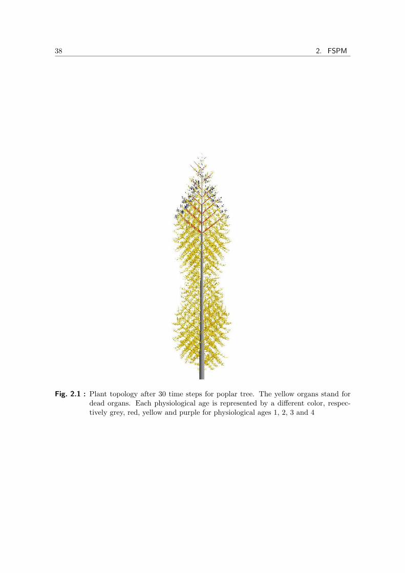
Fig. 2.1 : Plant topology after 30 time steps for poplar tree. The yellow organs stand fordead organs. Each physiological age is represented by a different color, respec-tively grey, red, yellow and purple for physiological ages 1, 2, 3 and 4

2.4. Introduction to several FSPMs 39
elementary units called phytomers that are gathered into categories according to mor-phological properties [Barthelemy and Caraglio, 2007]. These categories are indexedby a variable called physiological age, from 1 for the trunk to Pm for the small twigs.Pm is taken as 4 in our test case, which is generally sufficient to describe complextrees. A time step starts with the appearance of the new organs on the plant, and thetree architecture remains constant during the whole time step.
Interactions between plant organogenesis and functional mechanisms have beenimplemented by linking the number of new organs to the ratio of available biomassto plant demand. The main equations of the model are given in the following of thesection but a complete description can be read in [Mathieu et al., 2009]. Note howeverthat we restrict the study to a theoretical tree (with strong similarities in terms ofbehaviour with the poplar tree) and simplify the eco-physiological sub-models for thesake of clarity.
For the sensitivity analysis, the variable of interest is the amount of biomass pro-duced at each time step denoted by n. For this study, it is computed with a simpleempirical equation adapted from the Beer-Lambert law:
Q(n) = EPAR(n)µSp(1− exp−κ
Sf (n)
Sp ) (2.7)
EPAR(n) denotes the amount of photosynthetical active radiation received by theplant during the whole time step n, µ = 0.33 is an efficiency simulating the conversionof light energy into biomass, Sp is an empirical coefficient linked to the projectedground surface, κ denotes the extinction coefficient of the Beer-Lambert law. Sf (n)is the whole leaf surface area of the tree. It is the sum of each individual leaf surfacearea. Leaves are assumed to have a constant leaf mass per area e = 0.03g.cm−2,allowing to deduce their surfaces from their masses.
The amount of biomass Q(n) will be used for secondary growth and growth of newgrowth units and organs at the next time step. The allocation model is a proportionalone, which means that the biomass allocated to an organ is proportional to its sinkstrength divided by the plant demand, that is the sum of the organ sink strengths.The biomass used for the secondary growth is proportional to the number of leaves,in accordance with the pipe model theory [Shinozaki et al., 1964].
The number of functional buds, i.e. the ones that will give birth to new growthunits, and the number of phytomers on each branch depends on the ratio of availablebiomass to demand, see [Mathieu et al., 2009] for details . This key variable is corre-lated to the amount of biomass allocated to new organs denoted by QB(n). Finally,the tree leaf surface area is given by the equation:
Sf (n) =1
e
Pm∑
k=1
pkbSkBQB(n)
dkB ·Dfb(n)(2.8)

40 2. FSPM
pkb and SkB denote respectively the sink strength of buds and leaves of physiological
age k, dkB denote the demand of the corresponding growth unit and Dfb(n) is thedemand of these buds. For this case study, SB = 1, SI = 1 and SL = 0.1 denoterespectively the sink strengths for leaves, internodes and layers. They have the samevalues for each physiological age.
The plant behaviour is the result of the interactions between organogenesis andphotosynthesis. When there is enough available biomass, the ratio of biomass to de-mand is high and a lot of organs will appear in the tree. As the demand is proportionalto the number of organs, the increase in the number of leaves induces an increase inplant demand and consequently a decrease in the ratio of biomass to demand. Thenumber of new organs will decrease, inducing a low demand and a high ratio of biomassto demand, and so on. For some combination of the parameters, rhythms may appearin plant biomass production and topology [Mathieu et al., 2008].We choose such acase study for this thesis. Fig.2.1 shows the plant topology after 30 years.
Tab. 2.2 : GreenLab poplar tree: Distribution characteristics for uncertain parameters
Symbol Definition Mean value Uniform distribution
(SB)0 Sink blade PA=1 1 [0.9, 1.1](SB)1 Sink blade PA=2 1 [0.9, 1.1](SB)2 Sink blade PA=3 1 [0.9, 1.1](SB)3 Sink blade PA=4 1 [0.9, 1.1](SI)0 Sink Internode PA=1 1 [0.9, 1.1](SI)1 Sink Internode PA=2 1 [0.9, 1.1](SI)2 Sink Internode PA=3 1 [0.9, 1.1](SI)3 Sink Internode PA=4 1 [0.9, 1.1](SL)0 Sink Layer PA=1 0.1 [0.09, 0.11](SL)1 Sink Layer PA=2 0.1 [0.09, 0.11](SL)2 Sink Layer PA=3 0.1 [0.09, 0.11](SL)3 Sink Layer PA=4 0.1 [0.09, 0.11]µ Resistance blade 3 [2.7, 3.3]Sp Empirical coefficient 1.7 [1.53, 1.87]
2.4.3 NEMA model for wheat
Optimizing fertilizers’ use in agriculture requires being able to simulate nitrogen useby plants. Most crop models rely on the idea that a target nitrogen concentration intissues can be defined and that plants behave depending on the difference between thetarget and the actual nitrogen concentrations. However, such a target has never beenprecisely defined. Inputs of nitrogen fertilizers are fundamental to get high-yieldingcrops and a production of high quality with the required protein content. This requireda proper understanding of root N uptake regulation and of N determinism on yieldand production. Complex interactions exist between root N uptake, N remobilizationto grains, and photosynthesis, whose regulatory mechanisms remain far from clear.
NEMA, a functional-structural model of N economy within individual plants [Berth-eloot et al., 2011a], is developed for wheat after flowering to simulate Nitrogen content
2.5. Concluding remarks 41
of each photosynthetic organ and its remobilization following RubisCO turnover. Theturnover depends on light intercepted and a mobile nitrogen pool, which is enrichedby root uptake and nitrogen release from vegetative organs and depleted by grainuptake and protein synthesis in vegetative organs. It also accounts for the negativefeedback of circulating nitrogen on root uptake, which is formalized following HighAffinity Transport System (HATS) and Low Affinity Transport System (LATS) activ-ities. Organ nitrogen content and light intercepted determine dry matter productionby photosynthesis, which is distributed between organs according to their respectivedemand. This model has the specificity to integrate physiological processes governingN economy within plants: root N uptake is modeled following the HATS and LATS,and N is distributed between plant organs according to the turnover of the proteinsassociated to the photosynthetic apparatus. C assimilation is predicted from the Ncontent of each photosynthetic organ.
The NEMA scheme is presented in fig.2.2 and all the parameters involved in theparameters sensitivity analysis are listed in tab.2.3.
• Organogenesis ADEL-wheat [Fournier et al., 2003] [Bertheloot et al., 2011a].
• Distribution of nitrogen (N) : photosynthetic N, mobile N, structural N [Triboiand Triboi-Blondel, 2002], [Hafsi et al., 2000], [Bertheloot et al., 2008].
• Distribution of carbon (C) :(interaction with structural N, photosynthetic N)->GreenLab [Kang et al., 2008].
• Root Absorption [Drouet and Pages, 2007].
• Photosynthesis computed from incident radiations, surfaces of each leaf and itscontent in photosynthetic N [Evers et al., 2010].
2.5 Concluding remarks
• FSPMs aim to describe: Plant structural development (organogenesis and geom-etry), functional growth (biomass accumulation and allocation),and the complexinteractions between both. The complexity of the underlying biological pro-cesses, especially the interactions between functioning and structure [Vos et al.,2010], usually brings a lot of difficulties for experiment and modelling.
• Modelling usually follows principal steps. Generally, it includes development ofconcepts, experimentation and modelling.
• Sensitivity analysis plays important role to tackle the challenges FSPMs faces,like parameterization and model verification, and it may inspire new experimen-tation or adjustment of the model structure.

42 2. FSPM
Fig. 2.2 : NEMA: Overview of the model of N economy within wheat culms after flowering(Triticum aestivum L.)

2.5. Concluding remarks 43
Tab. 2.3 : NEMA: Model parameters: their symbols, definitions, and units. Organs in-cluded: grain(g), root(r), and 5 entities(tp): lamina, sheath, internode, peduncle,chaff.
Symbol Definition Unit
PAR interception(fixed value)
θLaAngle between the vertical and the vector
radiansnormal to the lamina plan
kvertical PAR extinction coefficient for vertical entities m2m−2
Root N uptake (5 parameters)
βC , βNCoefficient for C and N availability effect
dimensionlesson root N uptake
kr,1Constant of the Michaelis-Menten function reflecting
gm−3
HATS activity
kr,2Rate constant of the linear function reflecting
gm−3 Cd−1
LATS activity
(SMremr )min
Minimum threshold of dry matter influx intogday−1
roots to sustain root N uptake
Ur,maxTheoretical maximum root N uptake at
gm−3 Cd−1
saturating soil N concentration
N fluxes (28 parameters)1 for grain; 2 for root; 5 for each entity, 25 total for entities
δNr , δNtpRelative degradation rates of remobilizable N
Cd−1
for roots, entities tp
γRelative rate of potential grain N filling
Cd−1
during cell division
ktp,1, ktp,2
Michaelis-Menten constants defining gg−1, Jm−2d−1
photosynthetic N synthesis associated to xyleminflux for entities tp
pr, ptp,iProportion coefficient for N influx following dry
dimensionlessmass influx into roots, entities tp
σNph
tp,i
Relative rate of photosynthetic N synthesisgg−1 Cd−1
associated to xylem influx for entities tp
Tissue death and photosynthesis (15 parameters)3 for each entity, 15 total for entities
dtpProportion of maximum specific N mass at
dimensionlesswhich tissues die for entities tp
ωtp
Proportion coefficient linking photosynthesis atd−1saturating PAR and N mass per unit
photosynthetic areaǫtp Photosynthetic efficiency gJ−1
Dry matter fluxes (34 parameters)4 for grain; 5 for root; 5 for each entity, 25 total for entities
αg ,βg ,αr, Two parameters determining the shape of thedimensionless
βr,αtp,βtp Beta function for grains, roots, entities tp.
δMr ,δMtpRelative degradation rates of remobilizable
Cd−1
dry mass for roots, entities tpσMg ,σM
r ,σMtp,i Relative sink strength of grains, roots, entities tp dimensionless
ttMaccg ,ttMacc
r Duration during which grains, roots, entities tp CdttMacc
tp can accumulate dry mass

44 2. FSPM

3. SENSITIVITY ANALYSIS FOR FSPM
In this chapter we introduce the basic concepts, the methods and basic steps of sen-sitivity analysis. Definitions and equations of all algorithms of the SA applied in oursimulation are also given. Since uncertainty analysis (UA) and sensitivity analysis(SA) always come in tandem, we first introduce the general concept of UA and SAin section.3.1. The form of universal model definition is given in section.3.2, as oneimportant part of SA, issues about input factors are illustrated in section.3.3. Tomark the importance for the aims of SA, section.3.4 explicits this topic and specifiesthis issue in our work for FSPM, then we introduce the mathematical description ofthe main methods we used in our work: SRC and Sobol’s, especially several mean-ingful Sobol’s indices in section.3.5. Lastly, the basic steps of SA for FSPM is give insection.3.6.
3.1 Uncertainty analysis and sensitivity analysis
Most mathematical problems met in social, economic or natural sciences entail the useof mathematical models. A mathematical model is defined by a series of equations,input variables, parameters, and state variables to characterize the process being in-vestigated. The input is subject to many sources of uncertainty including errors ofmeasurement, absence of information and poor or partial understanding of the driv-ing forces and mechanisms. This uncertainty imposes a limit on our confidence in theresponse or model output, which is generally too complex for an easy appreciationof the relationship between input factors and output. The understanding of how themodel behaves in response to changes in its inputs, is of fundamental importance toensure a correct use of the models.
Good modelling practice requires that the modeler provides an evaluation of theconfidence in the model, possibly assessing the uncertainties associated with the mod-elling process and with the outcome of the model itself. Uncertainty and sensitivityanalysis offer valid tools for characterizing the uncertainty associated with a model.The goal of uncertainty analysis is to answer the question ‘what is the uncertaintyin y(x) given the uncertainty in x?’ and the goal of sensitivity analysis is to answerthe question ‘how important are the individual elements of x with respect to theuncertainty in y(x)?’ [Saltelli et al., 2006].
A possible definition of sensitivity analysis is the following: ‘The study of howuncertainty in the output of a model (numerical or otherwise) can be apportioned

46 3. Sensitivity analysis for FSPM
to different sources of uncertainty in the model input’[Saltelli et al., 2004]. Suchinformation given by SA may provide some help for model assessment:
• Measurement of model adequacy (e.g.does the model fit observation?)
• Knowledge of model relevance (e.g. is the model-based inference robust?)
• Identification of critical regions in the input space (e.g. which combination offactors corresponds to the highest risk?)
• Detection of interactions between factors
• Priorities for research and experimentations
• Simplification of model structure [Saltelli et al., 2004].
Thus the definition of sensitivity analysis involves models, model input and modeloutput. The following sections will present how these parts relate to the nature andpurpose of the model, as well as to the set-up of the uncertainty and sensitivityanalysis.
3.2 Model definition
Before starting sensitivity analysis, we give a definition of what is a ‘model’ in ourpractice. A model is represented by a mapping f (a deterministic or stochastic func-tion) which relates the inputs domain to the output space:
Y = f(X1, X2, · · · , Xk) (3.1)
The input factors (X1, X2, · · · , Xk) are supposed to be random variables described byidentified probability distributions which reflect the uncertain knowledge of the systemunder analysis, k is the number of factors involved, so we define the k dimensionalparameter vector X as one point in the space. Note that the model output Y undersensitivity analysis is always a scalar value. In the case of dynamic model output, theoutput is a vector for one state variable. We shall consider each scalar output valueof the vector in turn. As mentioned in Chapter.2, most of the FSPMs are dynamicmodels, the description of the state variables of plant growth evolving by time is themost important way of model presentation. So SA usually are performed separatelyat each calculation time step for FSPMs.
Consider a dynamic model represented by the following mathematical equation:
Y (t) = f(Z, θ, t) (3.2)
where Z is the vector of input variables of the model, θ is the vector of uncertainparameters and Y (t) is the model output at time t, for t ∈ 1, 2, · · ·T , the function

3.3. Model inputs 47
f(•) is the phenomenon studied and it is either deterministic or stochastic. Thestochastic aspect of the model will not be discussed in this thesis. However, it ispossible to take into account when making repetitions [Ginot et al., 2006], [Luretteet al., 2009].
Consider only the input variables and / or uncertain parameters of the modelwhich we call factors, we note that X, the model equation is written:
Y (t) = f(X, t) (3.3)
Eqn.3.3 corresponds to all our models of interest in this thesis. For FSPMs, simu-lations are usually computed at a daily time step and the sequential implementationof sensitivity analysis at each simulation date with one index per parameter per sim-ulation date. On one hand, it is one of the points we are interested in: the SA indicesevolving by time for factors can imply the stage evolution relating to plant growthactivities. One the other hand, when SA is performed separately at each time step forFSPMs, it can result in several hundreds of sensitivity indices. It is not easy to identifythe most important parameters based on such a large number of values. Moreover,this technique has the disadvantage of introducing a high level of redundancy becauseof the strong correlations between responses from one time step to the next. Likewise,intuitively, to screen one parameter, the requirement should be that the sensitivityresponse curve is always near zero at all time steps. However, we rarely get this kindof curve from our analysis. Therefore we devised a methodology that can deal with thescreening of parameters in this dynamic context, which will be discussed in Chapter.5.
For an easier and simpler way of presentation, next in this chapter, for all the math-ematic description about sensitivity analysis algorithm, we still stick to the conceptthat the output is a scalar as in eqn.3.1.
3.3 Model inputs
As we mentioned, we call the input variables and/or uncertain parameters as themodel input factors for SA. What constitutes an input for the analysis depends uponhow the analysis is set up. The inputs are those factors that are allowed to vary inorder to study their effect on the output. An obvious consequence is that the modellerwill remain ignorant of the importance of those factors which have been kept out of thescope. This is of course a hazard for the modeller, as a factor deemed non-influentialand kept fixed could haunt the results of the analysis at a later stage. Therefore,to choose a proper input factors group should be dealt with as carefully as possible.For us, we have gone an ‘expert review process’ for choosing the proper input factorsgroup. Two objectives were focused: the factors involved in the analysis should notbe too many, or else the analysis will be too complex with heavy computing cost; thefactors should neither be insufficient, or else the risk of of losing important informationwill come true.

48 3. Sensitivity analysis for FSPM
Assuming that we have observations and parameters which are estimated fromdata now, we might consider the model ‘true’ and run an uncertainty analysis bypropagating the uncertainty in the parameters through the model, all the way to themodel output. One way of doing this is through Monte Carlo analysis, in which wegenerate the samples of input according to the random distribution functions of theinput parameters, and derive from the propagations for the model output distribution.
Definition of the distributions DX1 , DX2 , · · · , DXkthat characterize the epistemic
uncertainty in factors X1, X2, · · · , Xk is also an important part of a sampling-baseduncertainty and sensitivity analysis. These distributions determine the input uncer-tainty that affect output Y .
Most of the time, the distributions of input factors are not easy to get. A possibleanalysis strategy is to perform an initial exploratory analysis with a rather crudedefinition for DX1 , DX2 , · · · , DXk
and use sensitivity analysis to identify the mostimportant analysis inputs. Then, resources can be concentrated on characterizingthe uncertainty in these inputs and a second presentation of decision-aiding analysiscan be carried out with these improved uncertainty characterizations [Helton et al.,2006b].
3.4 Purpose of sensitivity analysis
A few heuristic settings for SA, each corresponding to a specific stage or need of themodelling process, are suggested in [Saltelli and Tarantola, 2002] and [Saltelli et al.,2004]. As for all the scientific experiments, the first step is to be clear about the aimof the analysis which can lead to different practice strategies.
Generally, four aims can be classified for SA: Factor Prioritization (FP), FactorFixing (FF), Factor Mapping (FM) and Variance Cutting (VC) [Saltelli et al., 2008].
• Factor Prioritization: It is the identification of the most important factors. Ifthey are fixed to their true values, it would lead to the greatest reduction of theoutput variance. This setting can be used for the research prioritization, as itallows to identify those factors which deserve the most investment of researchattention in order to control the output variance to the minimum.
• Factor Fixing : It is the screening non-influential factors in the model, i.e. identi-fying those factors that can be fixed at any given value in their domains withoutsignificantly reducing the output variance. This setting is useful for model sim-plification to resolve the problem of over-parameterization, or when the modellerhas prior beliefs about the importance of some input factors, as it can help inproving or disproving a given model assumption.
• Variance Cutting : The reduction of the output variance to a lower threshold isperformed by simultaneously fixing the smallest number of input factors. This

3.4. Purpose of sensitivity analysis 49
setting could be useful when SA is part of a risk assessment study when aregulatory authority was to find the width of the impact estimate distributiontoo wide. The variance cutting and factor prioritization settings are very similarto each other, as they both aim at reducing the output variance. However, inthe case of factor prioritization the scope is to identify the most influent factorsone by one, while in the variance cutting setting the objective is to reduce theoutput variance down to a pre-established level by fixing the smallest subset offactors at once [Saltelli et al., 2004].
• Factor Mapping : Finally, the aim of SA can be to study which values of theinput factors lead to model realizations in a given range of the output space,e.g. above or below an assigned threshold. For example, the analyst wishes todivide the realizations of the Monte Carlo simulation into two groups, e.g. bycategorizing them as acceptable or non-acceptable. This setting can be carriedout using the Smirnov test and the approach is known as Regionalized SensitivityAnalysis [Hornberger and Spear, 1981].
FSPMs aim to describe plant structural development (organogenesis and geome-try), functional growth (biomass accumulation and allocation) and the complex in-teractions between both. sensitivity analysis provides a possible resolution for mostchallenges we are facing in functional-structural modelling:
• Knowledge Integration. Main integration is about structure and function andthe different time scales into one consistent modelling framework. For knowl-edge integration, SA can help for identifying important phases, key variables,important processes regarding some outputs, interaction between processes, be-tween parameters. It is corresponding to the Factor Priorization: by identifyingthe most important factors and interactions between them for the output un-der analysis, key biophysical processes relating to those factors can be marked;by identifying the most important function module (group of factors) and theinteraction between modules, the important interactions between processes canbe found.
• Link between models and the real world. It mainly relates to model parameteri-zation from experimental data which is one of the most important steps in modeldesign. This challenge is corresponding to Factor Prioritization and Factor Fix-ing: SA gives some guiding information about the priority of parameters we needto get from an experiment, the cost of an experiment can be more effectivelyarranged by adding more frequent measurements and more accurate study tothe ones with more contribution to the output variables, and vice versa; to sim-plify the complexity of parameter estimation, we need to cut down the numberof factors for this estimation, and one intuitive idea is to fix the non-influentialfactors identified by SA.
50 3. Sensitivity analysis for FSPM
3.5 SA methods
3.5.1 Classification of methods
There are a lot of classification standards for sensitivity analysis methods: accord-ing to the way how the method works, there are local and global methods [Cacuci,2003], [Cacuci et al., 2005], [Grievank, 2000]; according to the theoretical background,there are sampling-based methods [Helton et al., 2006a] and emulators-based meth-ods [Oakley and O’Hagan, 2004]; according to the purpose of SA, there are qualitativescreening methods like Morris method [Morris, 1991], [Campolongo et al., 2007] [Cam-polongo and Braddock, 1999] and quantitative ranking methods like Sobol’s method[Sobol, 1993].
The most common classifications of SA methods distinguish between quantitativeand qualitative methods and between local and global techniques.
• Qualitative methods are aimed at screening, while quantitative techniques canbe designed to give information on the amount of variance explained by eachfactor. In general, the choice of which method to use is driven by the computingcost, as local and qualitative methods are computationally less expensive [Saltelliet al., 2006].
• In local approaches (known as one-at-a-time, OAT), the effect of a single factor’svariation is estimated while keeping all the others fixed at their average values.Yet they cannot include the effect of the shape of the density functions of theinputs, and they are not model-independent.
• Global approaches estimate the effect on the output of a factor keeping all theothers varying. Generally, global approaches use model independent methodswhile not requiring assumptions of additivity or linearity. As a drawback, theyare usually computationally expensive [Cariboni et al., 2007].
Sampling-based approaches to uncertainty and sensitivity analysis are both effec-tive and widely used [Helton et al., 2006a], of which an important category of methodsare ‘Variance based’ methods. The basic concept for this kind of method is to de-compose the output variance into the contributions imputable to each input factor.The most widely used are the FAST (Fourier Amplitude Sensitivity Test, see [Cukieret al., 1973, 1978; Koda et al., 1979]), and Sobol’s methods, see [Sobol, 1993]. FASTmethod decomposes the output variance V (Y ) by means of spectral analysis. Sobol’smethod is based on the same decomposition of variance, which is achieved by MonteCarlo methods in place of spectral analysis. Since it is based on variance decompo-sition, the different types of sensitivity indices that it estimates can fulfill differentobjectives of sensitivity analysis: factor priorization, factor fixing, variance cutting orfactor mapping [Cariboni et al., 2007]. It is a very informative method but poten-tially computationally expensive [Helton et al., 2006a]. Besides the first-order effects,

3.5. SA methods 51
Sobol’s method also aims at determining the levels of interaction between parameters[Wu and Cournede, 2010]. Thus in our algorithm research and practice work in thisthesis, we mostly focused on Sobol’s method.
3.5.2 Description of methods
The simplest and most intuitive way to obtain a local sensitivity index is to com-pute derivatives (see [Grievank, 2000; Tomovic and Vukobratovic, 1972; Varma et al.,1999]). The sensitivity of the output Y to a perturbation of an input factor Xi isestimated at a given value X∗
i , as
Y′
Xi=
∂Y
∂Xi
∣∣∣Xi=x∗
i
(3.4)
In situations where Y and Xi have different range of uncertainties, a more bal-anced measure can be obtained normalizing the derivatives by the factors’ standarddeviations:
SσXi
=σ
Xi
σY
∂Y
∂Xi
∣∣∣Xi=x∗
i
(3.5)
The estimation of these OAT methods can be easily implemented, but they areinformative only if the model is linear/quasi-linear or if the range of uncertainty ofthe input factors is small [Cariboni et al., 2007].
The Standardized Regression Coefficients (SRC) method is based on the linearapproximation of the model and Monte Carlo simulations. SRC method can demon-strate the shape of the probability distribution of every factor. One important indexproduced by SRC is the model coefficient of determination R2, which represents thefraction of the output variance explained by the linear regression model itself. A sideresult of the model coefficient of determination (R2) is that it provides an indicator ofthe degree of non-linearity of the model. When R2 = 1, the system is linear and theSRCs can totally explain the variance of the output affected by each factor. Even whenmodels are moderately non-linear (i.e. > 0.9), the SRCs can provide valid qualitativeinformation. When getting small, the SRCs are no longer reliable sensitivity repre-sentations. In our practice, we call this model coefficient of determination linearityindex, and use it to assess the non-linearity of the model.
The SRCs are got based on model linear regression. When we make linear regres-sion for model Y = f(X), the result can be:
Y = b0 +k∑
i
bXiXi (3.6)
in which k is the number of the factors considered in SA, Xi denotes the factorsconsidered in SA, and b
Xiare the regression indices corresponding to each factor. To

52 3. Sensitivity analysis for FSPM
change these dimensioned coefficients values to the standardized ones, the SRC indexfor Xi denoted by γ
Xiis given by:
γXi
=σ
Xi
σY
bXi
(3.7)
in which σXi
and σYdenote respectively the standard deviation in Monte Carlo sim-
ulation for factor Xi and output Y . Note that if the factors are independent and thetrue model is linear, the summation of the squre value of γ
Xiequals to 1. Then the
following equation holds (see [Draper and Smith, 1981]):
∑
i
(γXi)2 = 1 (3.8)
∑i(γXi
)2 can therefore be considered as an index of the model linearity. This linearityof the system is described by the so called ‘model coefficient of determination’, whichis computed as:
R2Y =
∑N
d=1(Y∗ − µ
Y)2∑N
d=1(Y − µY)2
(3.9)
where µYis the mean value of Y in the Monte Carlo simulation, Y ∗ is the fitted value
in eqn.(3.6), Y is the actual value at each run, and N is the total number of runs.
The basic idea of Sobol’s method (see [Sobol, 1993]) is to decompose the functionof eqn.(3.1) into terms of increasing dimensionality:
f(X1, ..., Xk) = f0 +k∑
i=1
fi(Xi) (3.10)
+∑
1≤i<l≤k
fil(Xi, Xl)
+ · · ·+ f1,2,...,k(X1, ..., Xk)
If the input factors are mutually independent then there exists a unique decompositionof eqn.(3.10), such that all the summands are mutually orthogonal. The variance ofthe output variable Y can thus be decomposed into:
V (Y ) =k∑
i=1
Vi +∑
1≤i<l≤k
Vil + · · ·+ V1,2,...,k (3.11)
Where Vi, Vil, V1,2,...,k denote the variance of fi, fil, f1,2,...,k respectively.
Imagine if we fix factor Xi at its midpoint x∗i , how much would this change the
variance of Y ? We indicate the conditioned variance as:
VX−i(Y |Xi = x∗
i ) (3.12)

3.5. SA methods 53
where the variance is taken over parameter space X−i: a k − 1 dimensional vector ofall factors but Xi.
Comparing the variance V (Y ) in eqn.3.11, by fixing input factors based on eqn.3.12,we say that the smaller the conditional variance becomes, the more important Xi is,but it would make much difference where Xi is fixed. Further more, for non-linearmodels, fixing a factor might actually increase the variance instead of reducing it, alsodepending on where it is fixed.
The solution is to average eqn.3.12 over all possible values of Xi, which can bewritten:
EXi(VX−i
(Y |Xi)) (3.13)
From algebra theory, eqn.3.13 can be included in the equation as following:
EXi(VX−i
(Y |Xi)) + VXi(EX−i
(Y |Xi)) = V (Y ) (3.14)
Where VXi(EX−i
(Y |Xi)) is called the main effect of Xi on Y , and EXi(VX−i
(Y |Xi))the residual. Hence a small EXi
(VX−i(Y |Xi)) or a large VXi
(EX−i(Y |Xi)) will imply
that Xi is an important factor.
In this approach the first-order sensitivity index Si for factorXi defined in eqn.(3.1)is given by:
Si =VXi
(EX−i(Y |Xi))
V (Y )=
Vi(E−i(Y |Xi))
V (Y )(3.15)
where E and V indicate, respectively, the mean an variance operators, i indicates allpossible values of factor Xi, −i indicates all factors but Xi. The inner expectation istaken at a generic point in the space of variable Xi, while the outer variance is overall possible values of this generic point. According to eqn.3.11 and eqn.3.15, we caneasily refer that Si is a value always between 0 and 1. A high value of Si signals asignificant factor, but not vice versa. We will discuss this question again after all themain indices are introduced. Usually, Si is used for ‘Factor Priorization’ in SA, thevariables with high value of Si should have more priority for modelling investment.
Intuitively, the higher order sensitivity indexes Si1,...,is deduced from eqn.3.11should be:
Si1,...,is =Vi1,...,is
V (Y )
and we can also easily get the characteristic of all the sensitivity indices including allthe orders:
1 =k∑
i=1
Si +∑
1≤i<l≤k
Sil + · · ·+ S1,2,...,k (3.16)
It is interesting to write equations giving directly the high order indices of interest (asin eqn.3.15 for Si).

54 3. Sensitivity analysis for FSPM
Take second order for example, given two generic factors Xi and Xj (i 6= j), thefollowing result holds:
V (E(Y |Xi, Xj)) = Vi + Vj + Vij (3.17)
in which:
Vi = V (E(Y |Xi)) (3.18)
Vj = V (E(Y |Xj)) (3.19)
Vij = V (E(Y |Xi, Xj))− Vi − Vj (3.20)
We have dropped the indices of both the E and V operators. Indeed we do not needthem if we accept the convention that the argument conditioning the inner operator,Xi and Xj in this case, is also the set over which we apply the outer operator, i.e.the variance is taken over Xi and Xj, and the average E must be taken over allbut (Xi, Xj). The term Vij is the interaction term between factors Xi and Xj. Sothe second order index Si,j is the index that can describe the portion of the outputvariance represented by Vij:
Sij =V (E(Y |Xi, Xj))− Vi − Vj
V (Y )=
V (E(Y |Xi, Xj))
V (Y )− Si − Sj (3.21)
Eqn.3.21 gives us a clue that to get the second order index, we must first get thefirst order index of each factor involved. The higher order indices follow the sameidea: to compute any higher order index the requirement of all the lower order indicesis necessary. Though in [Saltelli, 2002], a strategy is proposed to make best use ofmodel simulations so that it would not be so computing cost heavy to get the higherorder indices. Generally, the higher order indices we want to get, the more modelsimulations we need, thus the heavier computing cost this brings. In Chapter.5, wewill illustrate a strategy of combining different lower order (typically) indices to avoidthis kind of high order index computing but still get the decomposition of the portionsof variances including them when necessary.
The higher order indices especially the second order ones, provide us with a way toevaluate the interaction between variables, from which we can deduce the biophysicalinteraction processes related to these variables.
Besides first order and high order indices, the total effect index is also frequentlyused for ‘factor screening’ [Saltelli et al., 2008] (that is to say to identify the leastinfluential parameters). To introduce it, we first consider another index called S−i
based on the definition in eqn.3.15 for first order index Si:
S−i =V (E(Y |X−i))
V (Y )=
V (E(Y |X1, X2, · · · , Xi−1, Xi+1, · · · , Xk)
V (Y )(3.22)
By analogy with the second order indices, eqn.3.22 should include all terms of anyorder that do not include factor Xi. As for eqn.3.16, the sum of all possible sensitivity

3.5. SA methods 55
terms must be 1, the difference 1 − S−i must be made up of all terms of any orderthat include Xi, we call it total order index, and denote it by STi:
STi = 1− V (E(Y |X−i))
V (Y )(3.23)
Again, according to the algebraic decomposition of V (Y ) in eqn.3.14, we also have:
STi =E−i(Vi(Y |X−i))
V (Y )(3.24)
Now we go back to the previous remark namely that ‘A high Si index signalsan important variable, but not vice versa.’ To process ‘Factor Fixing’, Si ≈ 0 is anecessary but insufficient condition for fixing factor Xi. This factor might be involvedin interactions with other factors such that, although its first-order term is zero, theremight be a non-zero higher order term. So it is meaningful to have a total order indexSTi for ‘Factor Fixing’, if STi = 0, then Xi is non-influent; reversely, if Xi is non-influent, the value of STi must be zero. STi = 0 (practically STi ≈ 0) is a necessaryand sufficient condition for Xi being non-influential.
To sum up, for a given factor Xi, we know from the value of first-order Sobol’sindex Si whether a factor is influent at the main effect, while an important differencebetween STi and Si flags an important role of interactions for that factor regardingoutput Y . If this is the case, inspection of the second order indices Sij for all i 6= jwill allow us to identify which factor Xi interacts with. Thus, in fact, besides thefirst-order effects, Sobol’s method also aims at determining the levels of interactionbetween parameters [Wu and Cournede, 2010].
Now we can extend the use of eqn.3.17 to a higher order. And we denote thevariance as V c
i1,i2,··· ,isin which ‘s’ is the number of factors included in this variance:
V ci1,i2,··· ,is
= V (E(Y |Xi1 , Xi2 , · · · , Xis)) (3.25)
Though we can not directly get the higher Sobol’s index that explains the inter-actions between parameters as Si1,i2,··· ,is from eqn.3.25, still it has its own meaningand it is useful when our objective is to investigate a group of parameters insteadof independent parameters. V c
i1,i2,··· ,isrepresents the variance donated by the set and
subsets of factors Xi1 , Xi2 , · · · , Xis: the variance caused by all the factors in thesets and all the interactions between these factors. As such, it evaluates the maineffect of the group of factors to the output.
In the case of complex system models that are composed of several sub-models (ormodules), we are interested in the sensitivity of these modules to the model output.Define the whole parameter space as a set P . Let Ω1,Ω2 . . .Ωr be a partition of P

56 3. Sensitivity analysis for FSPM
such that each subset Ωi = Xi1 , Xi2 , ..., Xis, corresponds to the set of parametersidentified as belonging to the ith module. We denote the first order group index ofsubset Ωi as S
gΩi, and i ∈ 1, 2, ..., r, the superscript ‘g’ means group index
SgΩi
=V ci1,i2,··· ,is
V (Y )=
V (E(Y |Xi1 , Xi2 , · · · , Xis))
V (Y )(3.26)
Similarly, V c−i1,i2,··· ,is
will indicate the sum of all indices in the complementary setof i1, i2, · · · , is, i.e. V c
−i1,i2,··· ,is= V c
l1,l2,··· ,lk−s, where ip 6= lq for all p ∈ [1, 2, · · · , s],
q ∈ [1, 2, · · · , k − s]. If we define a ‘total effect’ index for subset Ωi as in eqn.3.23 forone factor:
ST gΩi
= 1−V c−i1,i2,··· ,is
V (Y )= 1− V (E(Y |Xl1 , Xl2 , · · · , Xlk−s
))
V (Y )(3.27)
In the same way, if we define a second order group index for two subsets Ωi andΩj as in eqn.3.21 for two factors:
SgΩij
=V (E(Y |Ωi,Ωj))
V (Y )− Sg
Ωi− Sg
Ωj(3.28)
The total effect index ST gΩi
for subset Ωi means all the effects brought by the factorsset Xi1 , Xi2 , · · · , Xis: in the right side of eqn.3.16, it is the sum of all the terms ofany order that include at least one factor from the set, including the interactions ofall the subsets of these factors with the other ones that are not in Ωi.
In this sense, the difference ST gΩi−Sg
Ωimeans the interactions of the factors set with
the ones not belonging to the set. The second order group index SgΩij
specifically indi-cates the interactions between two subsets of factors. For a complex model in whichsubset of factors means the sub-module of the model, Sg
Ωijexplains the interaction
between two modules.
The group indices given here SgΩi, ST g
Ωi, Sg
Ωijand the difference ST g
Ωi− Sg
Ωiare
useful when the object we consider is a set of factors i.e. factors from one modulein the whole model. We will introduce a full methodology based on these indices inChapter.5 for module by module analysis and illustrate this practice in Chapter.7 forthe NEMA model.
3.6 Basic steps of SA for FSPM
Basically, SA of any model has to proceed in an orderly fashion. In practice thedevelopment of SA often proceeds in a loop of activities, because the modelers donot yet have enough knowledge about the attributes related to the decisions in SA,

3.6. Basic steps of SA for FSPM 57
including the range of parameters with uncertainty, lack of experimental data etc.The steps outlined below are more or less in a logical and chronological order, butthere are numerous reasons to deviate from the sequence that is presented.
1. It is the first step to establish the goal of sensitivity analysis and consequentlyto define the form of the output function that answers the question(s). As forFSPMs in our practice, ‘Factor priorization’ for modelling decision and ‘Factorfixing’ for model simplification are our two main aims of SA. Most of the time,what we called here ‘the output of the model’ is actually the state variablesof the model which play a very important role in the model. In our case, wemostly chose the total biomass production of each growth cycle as the output ofinterest for the two GreenLab models: maize and poplar tree, for the reason thatbiomass generation and allocation is the main formalism of GreenLab. What’smore, we also took the ratio of available biomass to total demand for poplartree, because it is representative of the level of trophic competition inside theplant. Thus it allows simulating as well the ontogenetic changes in plant topol-ogy throughout its growth phases (progressive set up of architecture units) asarchitectural plasticity in response to environmental changes. The interactionsbetween organogenesis and functioning can be detected by looking into this vari-able with sensitivity analysis. In the case of NEMA model, since it is far morecomplicated than the two previous models, the strategy we worked out is a littledifferent to the one we used for the first two GreenLab models. We will thereforetalk about this strategy called ‘module by module analysis’ in Chapter.5.
2. Nexgt we need to decide which input factors should be included in our analysis,that is to say, to define the parameter space for sensitivity analysis based on theobjective issue in the first step. At this level, trigger parameters can be defined,allowing one to sample across model structures, hypotheses, etc. Moreover, inthe case of multi-dimensional maps of factors, define the characterizing param-eters to represent them in the SA. After we decided the parameter space, it isto choose a distribution function for each of the input factors as mentioned insection.3.3. In our case, the distribution of parameters is a uniform distribution.
3. Afterwards, we need to choose sensitivity methods or to design the strategy if itmust be the combination of more than one SA methods. There are basically twoclasses of SA methods to decide: local methods and global ones. Local methodscannot include the effect of the shape of the density functions of the inputs,and they are not model independent but they are really computationally cheap.Global approaches estimate the effect on the output of a factor keeping all theothers varying. Generally, global approaches use model independent methodswhile not requiring assumptions of additivity or linearity. As a drawback, theyare usually computationally expensive [Cariboni et al., 2007]. The StandardizedRegression Coefficients (SRCs) can be viewed as an interesting trade-off betweenthe local and global method, regarding the advantages and shortcomings of both:the accuracy of the analysis and the computational cost. The main function ofSRCs we can make use of is the linearity index generalized by the determination

58 3. Sensitivity analysis for FSPM
coefficient. Alternatively, to fulfill our aim of ‘Factor Prioritization setting’ and‘Factor Fixing setting’ in our SA for FSPMs, we can choose Sobol’s method toget the index of Si and STi, because Sobol’s method can fulfill most the aims ofour analysis and can easily get the quantitative parameter interaction evaluationbased on the variance decomposition by Sij.
4. After all these preparations, the following is to start the Monte Carlo simulationsampling of the input factor for the analysis, then to evaluate the model on thegenerated sample and produce the output, which contains N (sampling number)output values.
5. Lastly, we analyse the model outputs using the estimators provided by the meth-ods we chose before and draw our conclusions based on the analysis result.
3.7 Concluding remarks
• Sensitivity analysis is the study of how uncertainty in the output of a model(numerical or otherwise) can be apportioned to different sources of uncertaintyin the model input [Saltelli et al., 2004]. SA involves models, model input andmodel output.
• Y (t) = f(X, t) corresponds to all our models of interest in this thesis. ForFSPMs, simulations are usually computed at a daily time step and the sequentialimplementation of sensitivity analysis at each simulation date with one index perparameter per simulation date. For an easier and simpler way of presentation,in all the mathematic description about sensitivity analysis algorithm next, westill stick to the concept that the output is a scalar as Y = f(X1, X2, · · · , Xk),k being the number of uncertain factors.
• Most of the time, the distributions of input factors are difficult to obtain. Apossible strategy is to perform an initial exploratory analysis with rather crudedefinition for the distribution of the inputs and use sensitivity analysis to identifythe most important inputs; then, resources can be concentrated on characterizingthe uncertainty of these inputs and a second sensitivity analysis can be carriedout with these improved uncertainty characterizations [Helton et al., 2006b].
• It is important to be clear about the aims at the beginning of SA: Factor Priori-tization (FP), Factor Fixing (FF), Factor Mapping (FM) and Variance Cutting(VC). In our practice, FP and FF is the case. Factor fixing is also called ‘factorscreening’ in some references, which means after identification of the least influ-ential factors, in the modelling processing that needs us to fix some factors totheir nominal value, they could be fixed.
• Determination coefficient R2 generated by the SRC method, first order indexSi, second order Sij, total order index STi, first order group index Sg
Ωi, total
order index ST gΩi, second order group index Sg
Ωijgiven by Sobol’s method are
the indices we mainly focused on in our work.

Part II
ALGORITHM AND METHODOLOGYDESIGN


4. AN EFFICIENT COMPUTATIONALMETHOD FOR GLOBAL SENSITIVITYANALYSIS
Sobol’s method decomposes the variance of the output of interest into terms due to in-dividual parameters but also to interactions between parameters. We are particularlyinterested in the later study on interactions between parameters using sobol’s method.Such information is crucial for models with potentially high levels of non-linearity andinteractions between processes, like plant growth models.
However, the computation of Sobol’s indices relies on Monte Carlo sampling andre-sampling, whose costs can be very high when model simulation is also expensive.Especially, for some complicated FSPMs, at organ level, the cost of model simulationcan be very heavy [Sievanen et al., 2000a]. Therefore, it is crucial to not only deviseefficient computing techniques, in order to make best use of model evaluations [Saltelli,2002], but also to have a good control of the estimation accuracy with respect to thenumber of samples.
The objective of this chapter is to study these two aspects. First, we propose acomputing method inspired by [Homma and Saltelli, 1996], which slightly improvestheir use of model evaluations, and then derive an estimator of the error of sensitivityindices evaluation with respect to the sampling size for this generic type of computa-tional methods. Numerical tests are then shown to illustrate the results. The methodis applied to the functional-structural models we have introduced in Chapter.2 whenSobol’s method is needed. For example, the GreenLab model for tree growth, whoseparticularity is the strong level of interaction between plant functioning and organo-genesis. The simulation result of the new method application to GreenLab tree modelwill be presented in Chapter.7.
4.1 Computation of sensitivity indices
4.1.1 General concepts of Sobol’s sensitivity analysis
We recall here the basic concepts of Sobol’s method [Sobol, 1993] to present the originalwork about sensitivity analysis indices. The function f(X) ≡ f(X1, X2, · · · , Xk) underinvestigation is defined in the k − dimensional cube Kk. If the input factors are

62 4. An Efficient Computational Method for Global Sensitivity Analysis
mutually independent then there exists a unique decomposition of f(X):
f(X1, ..., Xk) = f0 +k∑
i=1
fi(Xi) (4.1)
+∑
1≤i<l≤k
fil(Xi, Xl)
+ · · ·+ f1,2,...,k(X1, ..., Xk)
The basic idea of Sobol’s method (see [Sobol, 1993]) is to decompose the functionof interest into terms of increasing dimensionality as in eqn.(4.1), such that all thesummands are mutually orthogonal. The variance of the output variable Y can thusbe decomposed into:
V =k∑
i=1
Vi +∑
1≤i<l≤k
Vil + · · ·+ V1,2,...,k (4.2)
Where Vi, Vil, V1,2,...,k denote the variance of fi, fil, f1,2,...,k respectively.
In this approach the first-order sensitivity index for factor Xi is given by:
Si =VXi
(EX−i(Y |Xi))
V (Y )=
Vi(E−i(Y |Xi))
V (Y )(4.3)
where E and V indicate, respectively, the mean d variance operators, i indicates allpossible values of factor Xi, −i indicates all factors but Xi. The inner expectation istaken at a generic point in the space of variable Xi, while the outer variance is overall possible values of this generic point.
The complementary first order index S−i is given by:
S−i =V (E(Y |X−i))
V (Y )(4.4)
The second order sensitivity indexes Si1,...,is are given by:
Sij =V (E(Y |Xi, Xj))− Vi − Vj
V (Y )=
V (E(Y |Xi, Xj))
V (Y )− Si − Sj (4.5)
The total order effect STi is instead given by:
STi = 1− V (E(Y |X−i))
V (Y )(4.6)
If STi = 0, thenXi is non-influent, so the index STi is suitable for fixing non-influentialfactors. Standard Sobol’s method was proposed in [Sobol, 1993]. In [Homma andSaltelli, 1996], an improved estimator is presented to compensate the system error,completed in [Saltelli, 2002], and a computationally efficient design is discussed. Thismethod will therefore be called Homma-Saltelli method. We then propose an improve-ment of this method to promote its convergence characteristics.

4.1. Computation of sensitivity indices 63
4.1.2 Sobol’s computing method and Homma-Saltelli (H-S)
improvement
The standard Sobol’s method for SA was put forward in [Sobol, 1993], and the MonteCarlo procedure of Sobol’s index was first proposed by [Saltelli et al., 1993]. LetU = (Xi1 , Xi2 , · · · , Xis) and V = (Xl1 , Xl2 , · · · , Xlk−s
) be a partition of the k randomvariables corresponding to the input space. If we define:
Vu =
∫ ∫ ∫f(u,v)f(u,v′)DU(u)DV (v)DV (v
′)du dv dv′ (4.7)
with DU the probability distribution of random vector U (corresponding to parameteruncertainty) and DV the probability distribution of vector V. then:
V (E(Y |U)) = Vu − E2(Y ) (4.8)
The same argument, if:
V-u =
∫ ∫ ∫f(u,v)f(u′,v)DU(u)DU(u
′)DV (v)du du′ dv (4.9)
then:V (E(Y |-U)) = V-u − E2(Y ) (4.10)
We denote V (E(Y |-U) = V (E(Y |V) to note that V is the complementary vector ofU.
We take s = 1 which represents the computing for first order Sobol’s index. And asindicated in [Saltelli et al., 2010], ‘radial sampling’ should be applied to achieve better‘balance design’ in the sampling. We describe as following the numerical implemen-tation of Sobol’s index computing based on radial sampling. To get the conditionalexpectation value for model output Y , we first decide the base sampling dimensionN , then we implement the following steps:
1. Generate a Monte Carlo sampling of dimension N of the input factors accordingto their random distributions and form the N × k matrix UN×k (k being thedimension of the input space) with each row a set of parameters; UN×k is calledthe ‘sampling matrix’
UN×k =
x1(1) · · · xi(1) · · · xk(1)
x1(2) · · · xi(2) · · · xk(2)
.... . .
...x1(N) · · · xi(N) · · · xk(N)
(4.11)
2. Generate another sampling matrix of dimension N × k, WN×k, called the ‘re-sampling matrix’
WN×k =
x1(N+1) · · · xi(N+1) · · · xk(N+1)
x1(N+2) · · · xi(N+2) · · · xk(N+2)
.... . .
...x1(2N) · · · xi(2N) · · · xk(2N)
(4.12)

64 4. An Efficient Computational Method for Global Sensitivity Analysis
3. Define a matrix W ′N×k formed by all columns of WN×k, except the ith column
obtained from the ith column of UN×k,
W ′N×k =
x1(N+1) · · · xi(1) · · · xk(N+1)
x1(N+2) · · · xi(2) · · · xk(N+2)
.... . .
...x1(2N) · · · xi(N) · · · xk(2N)
(4.13)
4. Compute the model output for each set of input parameters from UN×k andW ′
N×k (that is to say for each row in UN×k and W ′N×k), to obtain two column
vectors of model outputs of dimension N : y = f(UN×k), y′R = f(W ′
N×k).
5. The sensitivity indices are hence computed based on scalar products of the abovedefined vectors of model outputs.
The applicability of the sensitivity estimates Si to a large class of functions f(X)is linked to the possibility of evaluating the multidimensional integral associated withthese estimates via Monte Carlo methods. For a given sampling size N tending to ∞the following estimate for the mean value of the output is straightforward:
f0 =1
N
N∑
j=1
y(j) (4.14)
where y(j) is the model output for a sample point in the parameter space Kk. Thehat symbol ‘’ will be used to denote estimates.
To list the estimator for the standard Sobol’s in [Sobol, 1993], the following nota-tion will be introduced:
V =1
N
N∑
j=1
y(j)2 (4.15)
V i =1
N
N∑
j=1
y(j)y′(j)R (4.16)
V −i =1
N
N∑
j=1
y(j)y′(j) (4.17)
Then we estimate the output variance by:
V = V − f 20 (4.18)
Vi(E−i(Y |Xi)) ≈ Vi = V i − f 20 (4.19)

4.1. Computation of sensitivity indices 65
V−i(Ei(Y |X−i)) ≈ V−i = V −i − f 20 (4.20)
and finally:
Si =Vi
V=
V i − f 20
V(4.21)
ST i = 1− V−i
V= 1− V −i − f 2
0
V(4.22)
As mentioned in [Homma and Saltelli, 1996], to compensate the ‘systematic error’in standard Sobol’s method, better estimates for the term Vi(E−i(Y |Xi)) is obtainedby also computing the output of the ‘re-sampling matrix’ WN×k, we denote it asyR = f(WN×k). We define γ2:
γ2 =1
N
N∑
j=1
y(j)y(j)R (4.23)
then the variance estimator is chosen as:
Vi(E−i(Y |Xi)) ≈ Vi = V i − γ2 (4.24)
For the same reason:
Si =Vi
V=
V i − γ2
V(4.25)
ST i = 1− V−i
V= 1− V −i − γ2
V(4.26)
In [Saltelli, 2002], a detailed proof of the cheaper computing cost for this methodis given, and one conclusion is that by adding the computational cost of N modelruns, we can get the full set of sensitivity indices (of all orders) for half the cost of thestandard Sobol’s method [Sobol, 1993]. For the Homma-Saltelli method, to estimateeach of the k first order indices, the computing cost is N(k + 2) model runs, with Nmodel runs for y, N model runs for yR and Nk model runs for y′
R. The same reasoningcan be applied for STi, see eqn.4.26. In the next section, we propose to adapt theHomma-Saltelli method in order to slightly improve the use of model evaluations.
4.1.3 A new method to compute Sobol’s indices
The attempt for the work is to promote the computing efficiency and convergence ofSobol’s method, and the basic idea is to to make the sampling-resampling processing‘smoother’ by ‘averaging’. In the Homma-Saltelli method, to compute E−i(Y |Xi),model outputs are computed for the N sampling matrix UN×k, N re-sampling matrix

66 4. An Efficient Computational Method for Global Sensitivity Analysis
Tab. 4.1 : Sobol’s Estimator improvement, H-S: Homma-Saltelli method [Homma andSaltelli, 1996]. y = f(UN×k), yR = f(WN×k), y
′ = f(U ′N×k), y
′R = f(W ′
N×k).
Variables H-S Proposed
f0 y(j) 12(y(j) + y
(j)R )
V i y(j)y′(j)R
12(y(j)y
′(j)R + y
(j)R y′(j))
V −i y(j)y′(j) 12(y(j)y′(j) + y
(j)R y
′(j)R )
V y(j)2 12(y(j)2 + y
(j)2
R )
γ2 y(j)y(j)R
12(y(j)y
(j)R + y′(j)y
′(j)R )
WN×k and for the changed ith column ‘re-sampling’ matrix (W ′N×k). The changed ith
column ‘sampling’ matrix U ′N×k can be defined and made full use of:
U ′N×k =
x1(1) · · · xi(N+1) · · · xk(1)
x1(2) · · · xi(N+2) · · · xk(2)
.... . .
...x1(N) · · · xi(2N) · · · xk(N)
(4.27)
We denote y′ = f(U ′N×k). Alternatively, y′ can also be used for E−i(Y |Xi). Cor-
respondingly, when we average these two ways of computing E−i(Y |Xi), then theouter Vi(E−i(Y |Xi)) should be inferior, because by doing the averaging, we will get amore ‘balanced’ simulation architecture. Thus, we obtain the proposed variant Sobol’sestimator as shown in table.4.1.
The computing cost is mentioned asN(k+2) for the old Sobol’s method to computeeach of the k first order indices [Pagano and Ratto, 2007]. For the estimator proposedin this paper, we make full use of the 2N samplings, just with Nk more model runs,that is to say with the computing cost of N(2k + 2) model runs. In order to fairlycompare the efficiency of the two computing methods, we need to ensure the samenumber of model evaluations. It is thus obtained if the sampling size in H-S methodand new method obey NH−S = Nnew ∗ 2(k + 1)/(k + 2).
Based on this new estimator configuration in table.4.1, we now extend this methodto second order index without adding extra model evaluation computing costs.
We rewrite the definition of second order index here:
Si1i2 =V (E(Y |Xi1 , Xi2))− Vi1 − Vi2
V (Y )=
V (E(Y |Xi1 , Xi2))
V (Y )− Si1 − Si2 (4.28)
According to eqn.4.7 and eqn.4.8, to compute V (E(Y |Xi1 , Xi2)), we can use thesame sampling and re-sampling matrix as in eqn.4.11 and eqn.4.12. Normally, likein eqn.4.13 and eqn.4.27 for the first order index computing, we should compute new

4.1. Computation of sensitivity indices 67
matrices for second order index computing as following:
W ′N×k,i1i2
=
x1(N+1) · · · xi(1)1
xi(1)2
· · · xk(N+1)
x1(N+2) · · · xi(2)1
xi(2)2
· · · xk(N+2)
.... . .
...x1(2N) · · · x
i(N)1
xi(N)2
· · · xk(2N)
(4.29)
U ′N×k,i1i2
=
x1(1) · · · xi(N+1)1
xi(N+1)2
· · · xk(1)
x1(2) · · · xi(N+2)1
xi(N+2)2
· · · xk(2)
.... . .
...x1(N) · · · x
i(2N)1
xi(2N)2
· · · xk(N)
(4.30)
in which i1 and i2 are the identities of the factors involved in the second order index.Considering factor set (Xi1 , Xi2) as factor subset u with s = 2, then f(W ′
N×k,i1i2)
equals to f(u,v′) in eqn.4.7. If we use the idea of our proposed new estimator for firstorder index mentioned before, the estimators should be:
Vu =1
2(f(UN×k)f(W
′N×k,i1i2
) + f(WN×k)f(U′N×k,i1i2
)) (4.31)
and
V-u =1
2(f(UN×k)f(U
′N×k,i1i2
) + f(WN×k)f(W′N×k,i1i2
)) (4.32)
However, if we check the matrix for first order as eqn.4.13 and eqn.4.27 in turn forith1 and ith2 factor respectively:
U ′N×k,i1
=
x1(1) · · · xi(N+1)1
xi(1)2
· · · xk(1)
x1(2) · · · xi(N+2)1
xi(2)2
· · · xk(2)
.... . .
...x1(N) · · · x
i(2N)1
xi(N)2
· · · xk(N)
(4.33)
W ′N×k,i1
=
x1(N+1) · · · xi(1)1
xi(N+1)2
· · · xk(N+1)
x1(N+2) · · · xi(2)1
xi(N+2)2
· · · xk(N+2)
.... . .
...x1(2N) · · · x
i(N)1
xi(2N)2
· · · xk(2N)
(4.34)
U ′N×k,i2
=
x1(1) · · · xi(1)1
xi(N+1)2
· · · xk(1)
x1(2) · · · xi(2)1
xi(N+2)2
· · · xk(2)
.... . .
...x1(N) · · · x
i(N)1
xi(2N)2
· · · xk(N)
(4.35)

68 4. An Efficient Computational Method for Global Sensitivity Analysis
W ′N×k,i2
=
x1(N+1) · · · xi(N+1)1
xi(1)2
· · · xk(N+1)
x1(N+2) · · · xi(N+2)1
xi(2)2
· · · xk(N+2)
.... . .
...x1(2N) · · · x
i(2N)1
xi(N)2
· · · xk(2N)
(4.36)
We can find that:
f(U ′N×k,i1
)f(W ′N×k,i2
) = f(UN×k)f(W′N×k,i1i2
) (4.37)
f(W ′N×k,i1
)f(U ′N×k,i2
) = f(WN×k)f(U′N×k,i1i2
) (4.38)
f(U ′N×k,i1
)f(U ′N×k,i2
) = f(UN×k)f(U′N×k,i1i2
) (4.39)
f(W ′N×k,i1
)f(W ′N×k,i2
) = f(WN×k)f(W′N×k,i1i2
) (4.40)
The ‘equal’ symbol in all the four equations means according to the Monte Carloprocedure for Sobol’s index, both sides have the same definition of computing givenin eqn.4.7 and eqn.4.9. Take eqn.4.37 for example, from the left side, matrix W ′
N×k,i2
has all the other factors ‘re-sampled’ but factor set (Xi1 , Xi2) comparing to matrixU ′N×k,i1
, while from the right side, matrix W ′N×k,i1i2
has all the other factors ‘re-sampled’ but factor set (Xi1 , Xi2) compared to matrix UN×k. The difference is thatfrom the right side, model simulation of matrix W ′
N×k,i1i2adds extra computing cost
when we have finished the first order index computing, while for the left side, allthe matrices involved have already got the model evaluations in the first order indexcomputing. So actually, by taking the left sides instead of the right sides in the secondorder index estimator, we can re-use the full sets of model evaluations necessary forfirst order index computing to compute the second order index. As we know that thecomputing cost of Sobol’s mainly comes from the model evaluations, in this ‘re-use’strategy of numerical implementation, 2 ∗ C2
k ∗N model evaluations can be saved, assuch to promote the computing efficiency by large.
The test result of the new method for first order index will be given in section.4.3.Before testing the estimator, we propose a way to evaluate the convergence charac-teristics of such type of computing methods.
4.2 Error estimation for Sobol’s method
4.2.1 Standard error, probable error
Assume function f(X) = f(x1, x2, ..., xk) under investigation is defined in the k−dimensionalrandom variable space, Monte Carlo method computing is applied to get the randomdistribution of f(X) with N sampling points, then standard error is:
σ(f) =1√N
√√√√ 1
N
N∑
n=1
f 2(Xn)− f 20 (4.41)

4.2. Error estimation for Sobol’s method 69
with the distribution mean value
f0 =1
N
N∑
n=1
f(Xn) (4.42)
and its variance
V (f) =1
N
N∑
n=1
f 2(Xn)− f 20 (4.43)
In [Homma and Saltelli, 1996], the use of the probable error δ corresponding tothe crude Monte Carlo method is computed like:
δf = 0.6745× σ(f) (4.44)
with the population f0 having 50% chance of falling in the interval f0 ± δf0. So,eqn.4.41 is the form we adopt for the error estimate.
Before we start for the probable error estimation of Si’s simulation result, we shouldmake sure that eqn.4.41 can be applied to our situation: first get the standard error ofthe considered variables, then we multiply the factor 0.6745 to get the probable error,based on the prerequisite that the variables should obey Gaussian distributions.
4.2.2 For Sobol’s formula
Error estimation is of crucial interest to check whether the SA computing has properlyconverged. Moreover, it can be used to give confidence bound of the result. Previouswork as in [Homma and Saltelli, 1996] gave interesting results for error estimation,but the conclusions are based on some restrictive assumptions:
• It assumes that the problem under analysis is scaled before computing the vari-ance, so that f 2
0 is small.
• The variance from f 20 is neglected based on condition 1), so the variances of V
and Vi are replace by V and Vi respectively.
We thus perform a more comprehensive error estimation without considering thesetwo hypotheses.
We take the H-S Sobol’s method for this error analysis. To get the error estimationfor the new computing method proposed in Section.4.1.3, we simply need to replacethe estimator in table.4.1 with the improved ones, and change the denominator fromN to 2N .

70 4. An Efficient Computational Method for Global Sensitivity Analysis
Error estimation for Si
Result 1: Approximation of the probable error for the computation of Si is given by:
δSi (4.45)
≈ 0.6745× σSi
= 0.6745×
√(σVi)
2
V 2+
V 2i (σV )2
V 4+ 2
Vi(σV )(σVi)
V 3
Proof : Here we rewrite the formula for Homma-Saltelli method to compute Sobol’sindices:
Si =Vi
V=
V i − γ2
V=
V i − γ2
V − f02
(4.46)
We need to evaluate the standard error of the four items: σV i, σV , σγ2 and σf02.
According to eqn.4.41 for the definition of standard error and eqn.4.14, eqn.4.16,eqn.4.15 eqn.4.23, for the computing of f0
2, V i, V , and γ2 respectively, then:
σV i =1√N
√√√√ 1
N
N∑
j=1
[(y(j)y
′(j)R )
2]− V
2
i (4.47)
σγ2 =1√N
√√√√ 1
N
N∑
j=1
[(y(j)y
(j)R )
2]− ((γ2)2) (4.48)
σV =1√N
√√√√ 1
N
N∑
j=1
[((y(j))2)2]− V2
(4.49)
σf0 =1√N
√√√√ 1
N
N∑
j=1
[(y(j))
2]− f 2
0 (4.50)
According to eqnA.6 in appendix, the variance for f 20 is:
Vf20= (σ(f 2
0 ))2= (2× f0 × σf0)
2(4.51)
So:
σ(f 20 ) = (2× f0 × σf0) (4.52)
and using the eqnA.8 giving the variance of a sum of random variables:
σV =√
VV + Vf20− 2cov(V , f 2
0 ) (4.53)

4.2. Error estimation for Sobol’s method 71
Since V and f 20 use the same set of samples, the correlation index ρ can be ap-
proximated to be 1 here, so:
cov(V , f 20 ) = ρ
√VV
√Vf20≈√
VV
√Vf20= σV σ(f 2
0 ) (4.54)
Then:
σV ≈√
(σV )2 + (σ(f 20 ))
2 − 2σV σ(f 20 )
≈∣∣∣σV − σ(f 2
0 )∣∣∣
so:
σV ≈∣∣∣σV − σ(f 2
0 )∣∣∣
≈
∣∣∣∣∣∣
√√√√ 1
N
(1
N
N∑
j=1
[((y(j))2)2]− V2
)
− 2× f0 × σf0
∣∣∣
Likewise, for σSi with Vi = V i − γ2, and correlation coefficient of V i and γ2 set to1:
σVi ≈∣∣σV i − σγ2
∣∣ (4.55)
We then use eqnA.10 given in appendix to estimate the variables of Vi
V, but we have
the same problem to get the correlation index of Vi and V , and it is not 1 anymore,because they don not share the same sample. However, to make sure that we will getthe ‘upper bound’ of the real variance, we consider the least favorable case, obtainedfor a correlation of -1, that is to say: cov(Vi, V ) ≈ −σV σVi and then:
σSi =
√(σVi)
2
V 2+
V 2i (σV )2
V 4+ 2
Vi(σV )(σVi)
V 3(4.56)
according to eqn.4.44 about the relationship between probable error and standarderror,So:
δSi (4.57)
≈ 0.6745× σSi
= 0.6745×
√(σVi)
2
V 2+
V 2i (σV )2
V 4+ 2
Vi(σV )(σVi)
V 3

72 4. An Efficient Computational Method for Global Sensitivity Analysis
error estimation for STi
Result 2: Approximation of the probable error for the computation of STi is givenby:
δST i (4.58)
≈ 0.6745× σST i
= 0.6745×
√(σV−i)
2
V 2+
V 2−i(σV )2
V 4+ 2
V−i(σV )(σV−i)
V 3
Proof : As we check eqn.4.26, we can get that the error estimation for STi is similaras for Si, the difference is changing σVi to σV−i and changing Vi to V−i in eqn.errSi,and we can easily get that:
σV −i =1√N
√√√√ 1
N
N∑
j=1
[(y(j)y′(j))
2]− V
2
−i (4.59)
so as in eqn.4.55:σV−i =
∣∣σV −i − σγ2∣∣ (4.60)
finally:
δST i (4.61)
≈ 0.6745× σST i
= 0.6745×
√(σV−i)
2
V 2+
V 2−i(σV )2
V 4+ 2
V−i(σV )(σV−i)
V 3
4.3 Computational Tests
4.3.1 Analytical functions
To demonstrate the performance of the error estimation and the efficiency of the pro-posed method, an artificial analytical model with 3 input variables (Ishigami Function)is considered, as in [Ishigami and Homma, 1990]:
f(X1, X2, X3) = sinX1 + asin2X2 + bX34sinX1 (4.62)
where its input probability density functions (pdf) is as follows:
pi(Xi) =
12π, −π ≤ Xi ≤ π
0, Xi < −πorXi > πi = 1, 2, 3
from eqn.4.2, the total variance V and partial variances Vi can be obtained analyticallyas:
V =a2
8+
bπ4
5+
b2π8
18+
1
2(4.63)

4.3. Computational Tests 73
V1 =bπ4
5+
b2π8
50+
1
2(4.64)
V2 =a2
8(4.65)
V3 = 0 (4.66)
In our test case, the constants in eqn.4.63, 4.64, 4.65, 4.66 are given the values a = 7and b = 0.1. We use the ‘Mersenne Twister random number generator’ to get therandom sampling for the 3 input parameters.
4.3.2 error estimation test
The purpose of this test is to examine how the error estimation works in the MonteCarlo computation of sensitivity with the comparison between the ones computedanalytically from eqn.4.45, eqn.4.58 respectively for δSi, δSTi and those obtained byrepeating the computation of SA indices for a number of times (with different seeds
for the MT generator) are denoted by δSi
∗
, δSTi
∗
. NbR will denote the number ofrepetitions. All the data shown here are calculated using combined data from all runs.We use the Homma-Saltelli Sobol’s estimator in this test case in order to compare theerror estimation with those obtained in the previous works in [Homma and Saltelli,
1996], denoted by δSiref , δSTiref .
Since the set of all Si plus the set of all STi give a fairly good description of themodel sensitivities, here we only give these two sets of indices for the test.
As shown in table.4.2 and table.4.3, we can see that the theoretical upper bounderror estimation δSi, δSTi is very effective compared to the one we computed by
numerical simulations δSi
∗
, δSTi
∗
, while it is much more accurate than the previous
work δSiref , δSTiref . So the proposed error estimation can be a good indication tojudge the level of accuracy of the SA index computation, according to which we canfind a proper number of sampling (NbS) for SA.
4.3.3 Comparison of H-S and proposed method
We compare the Homma-Saltelli (H-S) method and the proposed new one in table.4.4and table.4.5, with the same model evaluation computing cost corresponding to dif-ferent numbers of samplings as explained in Section.4.1.3. As we mentioned in sec-tion.4.1.3, NH−S = Nnew ∗ 2(k + 1)/(k + 2), here k = 3 for our test case, whenNnew = 1000, then NH−S = 1600. We can see that, both for Si or STi, our proposednew method can provide more stable results, that is to say, it can get the result withless variance, as also confirmed by our standard error estimation. This result agreeswith our expectation that the complimentary characteristic of the sampling matrixand re-sampling matrix can help to get a more ‘balanced’ result. Other types of esti-mators for Sobol indices exist in the literature. In a recent paper [Saltelli et al., 2010],

74 4. An Efficient Computational Method for Global Sensitivity Analysis
Tab. 4.2 : H-S Sobol’s method for Si, same Number of Runs(NbR=100), different Numbersof Samplings(NbS)
NbS=10
Variables Si(exact) Si Bias δSi δSiref δSi∗
X1 0.3138 0.332128893 0.018328893 0.420126891 0.64922391 0.394116208
X2 0.4424 0.576970598 0.134570598 0.441915034 0.799264515 0.459467686
X3 0 -0.047977424 0.047977424 0.368651048 0.40482392 0.329106545
NbS=100
Variables Si(exact) Si Bias δSi δSiref δSi∗
X1 0.3138 0.317898441 0.00409844 0.113155712 0.17496605 0.098588362
X2 0.4424 0.44332627 0.00092627 0.110788108 0.19688452 0.072259899
X3 0 0.014475517 0.014475517 0.126772756 0.129683521 0.082991208
NbS=1000
Variables Si(exact) Si Bias δSi δSiref δSi∗
X1 0.3138 0.31704138 0.00324138 0.035478791 0.056020475 0.029357167
X2 0.4424 0.44426211 0.00186211 0.034121285 0.062915907 0.029415413
X3 0 0.003420994 0.003420994 0.040333006 0.040555193 0.02417304
the authors compared different types of estimators for STi, and Jansen’s [Jansen,1999] estimator is shown to be the most efficient. It would thus be interesting toadapt the strategy proposed in this paper to other estimators to check whether thesame convergence characteristics can be obtained.
4.4 Discussion
With the objective of an efficient computational method for sensitivity analysis offunctional-structural tree growth models, we proposed a new estimator based onHomma-Saltelli method to compute Sobol’s indices. This new estimator can be con-sidered as an effort to improve the efficiency of SA methods for models.
Another problem brought by this sampling-based computing strategy is to getresults as accurate as possible but with as few samples as possible. We generally lackbenchmarks to control the convergence of computing methods. Most of the time wedo not have the analytical result for the sensitivity indices. Therefore, we derived atheoretical analysis of the error estimation for the sensitivity analysis for the class ofSobol’s estimators (it can be applied to all the three Sobol’s estimators mentioned inthis paper). An analytical test function is used to test the error estimation, and weobtained that the error estimation in this paper gives out a better ‘upper bound’ thanthe previous works related to this problem. This error estimation directly relates tothe variance of the result, so it can also be used for checking the confidence interval,which is usually difficult to attain.
The computation method for Sobol indices as well as the error estimation can also

4.4. Discussion 75
Tab. 4.3 : H-S Sobol’s method for STi, same Number of Runs(NbR=100), different Num-bers of Samplings(NbS)
NbS=10
Variables STi(exact) STi Bias δSTi δSTiref δSTi∗
X1 0.5574 0.471006778 0.086393222 0.587139075 0.773255643 0.452078804
X2 0.4442 0.433857546 0.010342454 0.470375601 0.80001505 0.419140296
X3 0.241 0.09090012 0.15009988 0.518931875 1.04536509 0.45891867
NbS=100
Variables STi(exact) STi Bias δSTi δSTiref δSTi∗
X1 0.5574 0.54219821 0.01520179 0.123465946 0.21247326 0.11183428
X2 0.4442 0.457708634 0.013508634 0.126828544 0.23284288 0.08433098
X3 0.241 0.238775324 0.002224676 0.1248745 0.26201749 0.114110644
NbS=1000
Variables STi(exact) STi Bias δSTi δSTiref δSTi∗
X1 0.5574 0.55231685 0.00508315 0.038581076 0.067597875 0.037170484
X2 0.4442 0.43980209 0.00439791 0.040345109 0.076681373 0.028618586
X3 0.241 0.23869646 0.00230354 0.035262641 0.084598942 0.034681808
Tab. 4.4 : Efficiency comparison of H-S and our new Sobol’s method for Si, withthe same number of model evaluations, H-S method with Number of Sam-plings(NbS=1600), Number of Runs(NbR=100), new method with Number ofSamplings(NbS=1000), Number of Runs(NbR=100)
H-S
Variables Si(exact) Si Bias δSi δSiref δSi∗
X1 0.3138 0.31533298 0.00153298 0.02799958 0.044172429 0.022979037
X2 0.4424 0.44665802 0.00425802 0.027065163 0.049959473 0.020148217
X3 0 -0.000991375 0.000991375 0.031977602 0.031926896 0.018688355
New
Variables Si(exact) Si Bias δSi δSiref δSi∗
X1 0.3138 0.31298693 0.00081307 0.024947723 0.051779454 0.014254
X2 0.4424 0.44600325 0.00360325 0.024195279 0.062443818 0.014995118
X3 0 -0.000171562 0.000171562 0.028633187 0.02861765 0.01049768

76 4. An Efficient Computational Method for Global Sensitivity Analysis
Tab. 4.5 : Efficiency comparison of H-S and our new Sobol’s method for STi, withthe same number of model evaluations, H-S method with Number of Sam-plings(NbS=1600), Number of Runs(NbR=100), new method with Number ofSamplings(NbS=1000), Number of Runs(NbR=100)
H-S
Variables STi(exact) STi Bias δSTi δSTiref δSTi∗
X1 0.5574 0.55433338 0.00306662 0.030524063 0.053367661 0.028061632
X2 0.4442 0.44145391 0.00274609 0.031846525 0.060492716 0.024130443
X3 0.241 0.24447647 0.00347647 0.027831009 0.066898161 0.02334635
New
Variables STi(exact) STi Bias δSTi δSTiref δSTi∗
X1 0.5574 0.55543245 0.00196755 0.027455945 0.065578754 0.018760671
X2 0.4442 0.44419771 2.29E-06 0.028548756 0.076191397 0.01669605
X3 0.241 0.23800909 0.00299091 0.024822554 0.089599272 0.022789275
be performed with other types of random number generator which are proved to alsohave an important influence on the efficiency of the algorithms [Saltelli et al., 2010],therefore, same tests were performed with quasi-random generator [Saltelli et al., 2010]leading to the same conclusions.

5. STRATEGY DESIGN
In the previous chapter, we present our work on the computational issue of Sobol’smethod, which is the first important issue in our thesis. In this chapter, we focuson the second issue we proposed at the beginning of this thesis: the strategy designof SA for FSPMs. We first give a general view of this topic in section.5.1. Wemainly introduce the strategy design in two aspects: non-linearity assessment fromSRC method in section.5.2 and the more general methodology for full SA of complexbiophysical models in section.5.3.
5.1 Introduction
A good sensitivity analysis practice does not only needs well designed SA estimators(as in the previous chapter) but also needs good understanding of how to compre-hensively use more than one methods to make them be complementary to each othersince different methods tackle different issues of interest. This is what we consider as‘strategy design’.
Though pointed out in [Saltelli et al., 2004], one property of an ideal sensitivityanalysis method is that it should be ‘model independent’, which means a methodshould work regardless of the attributes of the model itself like additive, linear, etc.However, the strategy design is necessary in our work of sensitivity analysis for FSPMs.More work needs to be done for exploring how global sensitivity analysis can help inthe parameterization of FSPM, by quantifying the driving forces of the phenomenadescribed by the models and the relative importance of the described biophysicalprocesses regarding the outputs of interest.
As we have mentioned in the performance steps of SA in section.3.6, the strategydesign includes:
• To choose a proper sensitivity analysis method to fulfill different aims.
• To combine more than one SA method in order to make best use of each method’sadvantages and to make them complementary to each other.
For the first type of issue, in Chapter.3, we have already recalled that:
• Basically we can choose between local methods and global methods. Local meth-ods cannot include the effect of the shape of the density functions of the inputs,

78 5. Strategy design
and they are not model independent but they are really computationally cheap.Global approaches estimate the effect on the output of a factor keeping all theothers varying. Generally, global approaches use model independent methodsand do not require assumptions of additively or linearity. As a drawback, theyare usually computationally expensive [Cariboni et al., 2007]. So it depends onour knowledge about the properties of the model and the computing cost we canafford.
• The Standardized Regression Coefficients (SRCs) can be viewed as an interest-ing trade off between local and global method, regarding the advantages andshortcomings of both: the accuracy of the analysis and the computing cost.The determination coefficient computed by SRCs can be used in non-linearityassessment for models.
• Alternatively, to fulfill our aim of ‘Factor Prioritization setting’ and ‘FactorFixing setting’ in our SA for FSPMs, we can choose Sobol’s method to getthe first order index of Si and total order index STi. Moreover, with Sobol’smethod, we can get the quantitative parameter interaction evaluation based onthe variance decomposition by Sij. For a given factor Xi, the value of first-orderSobol’s index Si indicates that whether a factor is mainly influent, while animportant difference between STi (Total order effect) and Si flags an importantrole of interactions for that factor in output y(t). In this case, inspection of thesecond order index Sij for all i 6= j will allow us to identify which factor Xi
interacts with.
• The group indices given in section.3.5.2: SgΩi, ST g
Ωiare useful when our objective
is to analyze the effect of a subset of factor (usually factors from one moduleor sub-model in the whole model) to the output variance, and the differenceST g
Ωi− Sg
Ωimeans the interactions of the set of factors with those that do not
belong to the set. SgΩij
specifically indicate the interactions between two subsetsof factors.
Complex biological models are uaually characterized by several interacting pro-cesses with sub-models describing each of them. Most FSPMs are such models. It isinteresting to evaluate the importance of the sub-models (usually ‘function’ modulescorresponding to the biophysical processes they describe) by sensitivity analysis. Forthis objective, in practice we need to firstly classify the parameters into different bio-logical function modules according to the biologist modeller’s expert knowledge, thento check the joint sensitivity effects of the groups of parameters that belong to thosemodules. This is how ‘module-by-module’ analysis for complex biophysical system isput forward. The strategy design should be divided into several steps for which wechoose different SA methods to fulfill different requirements.
The choice of a proper sensitivity analysis method to fulfill different aims of dif-ferent sub-steps of the analysis faces the same SA general issues as mentioned before.

5.2. SRC method and non-linearity assessment 79
However, module-by-module analysis requires us to make the combination of morethan one SA method in order to make best use of each method’s advantages and tomake them complementary to each other. We will propose a module by module anal-ysis for complex FSPMs inspired by the strategy in [Ruget et al., 2002] in section.5.3.
5.2 Standardized Regression Coefficients (SRC) method andnon-linearity assessment
Plants are known as complex systems with a strong level of interactions and compen-sations, and one of the aims of FSPMs is to describe and understand this complexity.As such, non-linearity is expected to play a key role in the study. The knowledge ofthe intrinsic non-linearity of the model and of its dynamic evolution throughout plantgrowth is very useful for the study of model behavior and properties, to underline theoccurrence of particular biological phenomena or to improve the statistical analysiswhen confronting models to experimental data (e.g. statistical properties of estimatorsor numerical methods to compute the propagation of errors [Julier et al., 2000]).
As detailed in Chapter.3, the Standardized Regression Coefficients method is basedon a global linear approximation of the model. It provides the model coefficientof determination R2, which represents the fraction of the output variance explainedby the linear regression model itself. When R2 = 1, the system is linear and theSRCs can totally explain the variance of the output affected by each factor. Evenwhen models are moderately non-linear (i.e. R2>0.9), the SRCs can provide validqualitative information. When it gets small, the SRCs are no longer reliable sensitivityrepresentations. To be more direct, we call this model coefficient of determinationlinearity index, and use it to assess the non-linearity of the model.
The objective of this section is thus to explore the level of linearity of the 3 FSPMsintroduced in Chapter.2, which have different levels of complexity, and infer in eachcase what information can be drawn from this analysis.
We recall here generally the three FSPMs involved in this work. Firstly a simplesource-sink model of maize growth, which is used to specifically study the process ofcarbon(C) allocation among expanding organs during plant growth, with simple plantstructure, multi-stage and detailed observations, secondly the GreenLab model of treegrowth (applied to poplar tree) characterized by the retroaction of plant functioningon its organogenesis [Mathieu et al., 2008], which describes tree structural plasticity inresponse to trophic competition, lastly a functional-structural model, NEMA [Berth-eloot et al., 2011a], describing C and nitrogen (N) acquisition by a wheat plant as wellas C and N distributions between plant organs after flowering.
In this study, we follow dynamically the linearity index throughout plant growth.In the models of the GreenLab type, the output of interest for the SA is the biomass

80 5. Strategy design
Fig. 5.1 : GreenLab Maize (a)At each GC, biomass allocation per organ type (b)Evolutionof the linearity index
production at each GC, and in the NEMA model, grain dry mass, grain N mass androot N uptake are considered.
The linearity analysis for the biomass production for GreenLab Maize is given infig.5.1.b. A non-linear period is denoted by the minimum around GC17. It is a keystep in terms of biophysical processes corresponding to the transition between twoallocation phases, the first one corresponding mostly to leaf area increase and thesecond one to grain filling (as illustrated by fig.5.1.a showing the biomass allocationto each type of organ).
For the poplar tree model with retroaction of functioning on organogenesis, fig.5.2.ashows the evolution of the ratio for biomass production to organs’ demand whichis the key variable controlling tree organogenesis. The linearity index is shown infig.5.2.b. The initial states show high linearity indices, but these decrease rapidly withthe increasing influence of the trophic competition on organogenesis, particularly theappearance of the first branch at growth cycle 5. The linearity index stabilizes ataround 0.5, which is quite low, showing the importance of retroaction in the dynamicsystem.
For the model of C-N dynamics (NEMA), the evolutions of the linearity indicesfor N mass of the grains, their dry mass and the rate of root N uptake are shown infig.5.3. If the model is highly linear for the grain dry mass fig.5.3.a, it is not the casefor grain Nitrogen mass fig.5.3.b. For N uptake by root fig.5.3.c, the evolution of thelinearity index is hierachical with a low level of linearity. It seems reasonable when weconsider the complex driving forces for N uptake in the model, involving the functionof the nitrate concentration in the soil modulated by positive and negative feedbacksof respectively C and N in the plant, on root activity.
Considering the dynamic evolution of the linearity index throughout plant growthmay reveal phases during which linearity is very high, probably showing some stable

5.2. SRC method and non-linearity assessment 81
Fig. 5.2 : Poplar tree model with retroaction of functioning on organogenesis: (a) Evolutionof ratio of available biomass to organs’ demand (Q/D) (b) Evolution of linearityindex
Fig. 5.3 : NEMA: Evolution of the linearity index for different outputs (a) Dry mass of thegrains (b) Nitrogen mass of the grains (c) Root N uptake

82 5. Strategy design
behavior for which the experimental process for parameter estimation could be lighter.On the contrary, the analysis may show evidence of some moments when a strongnon-linearity occurs. Such moments may be characteristic of very specific biologicalphenomena during plant growth as well as the high level of interactions betweenparameters, either known by the modeler or unknown, in which case they shouldprobably be investigated more. For non-linear phases, a special care should be takenof with respect to the frequency and details of experimental measures.
For example, since the parametric estimation of GreenLab by model inversionrelies on multi-stage observations, the information given by the linearity analysis canbe taken advantage of. For maize, it is important to have detailed and frequentobservations between cycles 14 and 20, while the measurements can be lighter aftercycle 20. For the poplar tree model, the high level of non-linearity is coupled with thedifficulty to get regular observation data (due to the time scale and the inventmentlevel of experiments). The linearity analysis should thus be coupled with a full SA tohelp us define a proper strategy for parameter estimation: for example, in two steps asproposed by [Letort et al., 2008a] first consider the observed topology as fixed to getthe functional parameters, and then estimate the parameters driving the retroactionof functioning on organogenesis.
For complex bio-physical models like NEMA, we expect a strong genetic determi-nant of model parameters. One of the interests of assessing the level of model linearityis that non-linear phases are characterized by a high level of interactions between pa-rameters. When model parameters are genetic, understanding and quantifying this in-teraction is crucial in the objective of using plant models as an intermediate to developa predictive capacity from genotype to phenotype [Hammer et al., 2006; Buck-Sorlinand Bachmann, 2000] and design ideotypes. If a parameter has little interaction withothers, we can directly concentrate on this trait for the design of ideotypes [Qi et al.,2010]. If the interaction is strong, it is more complex. If the parameters are stronglygenetically related (determination by the same genes), the model parameterizationshould be improved to take into account this fundamental interaction. If they arenot genetically related, breeding strategy should rely on multi-dimensional optimiza-tion to handle the interacting processes. The next objective of our study is thus touse Sobol’s method [Sobol, 1993] to explore the interactions between processes andparameters for this model.
5.3 A methodology for complex biophysical models
Complex biological models are usually characterized by sub-models describing severalinteracting processes respectively. Most FSPMs are such models. It is interesting toevaluate the importance of the sub-models (usually ‘function’ modules correspondingto the biophysical processes they describe) by sensitivity analysis. For the objective,in practice we need to firstly classify the parameters into different biological functionmodules according to the biologist modeller’s expert knowledge, then to check the joint

5.3. A methodology for complex biophysical models 83
sensitivity effects of the groups of parameters that belong to those modules. This ishow ‘module-by-module’ analysis for complex biophysical system is put forward. Thestrategy design should be divided into several steps for which we choose different SAmethods to fulfill different requirements.
Our proposed methodology for module by module analysis is inspired by [Rugetet al., 2002], in which analysis was made in two steps: first, within each meta-process(module), the most important parameters are identified; then sensitivity to identifiedparameters is calculated taking into account together all meta-processes. A certainnumber of parameters (according to empirical information) are selected from eachmodule for the analysis. The influence of parameters inside their own modules wasstudied through response surface methodology, in order to give sensitivity values link-ing outputs and parameters and to choose the most representative parameter of eachmodule to use in the intermodule analysis. To do the internal analysis of each module,they sampled the parameters selected for this module according to their distributionswhile fixing the parameters in all the other modules to their mean values, then theparameter samples are used for the regression surface functions to resolve the indices.Afterwards, they did the internal modules analysis: using response surface methodwith all the parameters selected from each module in the previous step.
However, there are several drawbacks for this strategy:
• There are a lot of limitations for using the regression method. First, strictrequirements have to be fulfilled for the model functions like linear, additive, orfor surface response, the model has to be a continuous system, for FSPMs thisrequirement can not always be satisfied. Besides, only second order ‘interaction’has been found in [Ruget et al., 2002]. The higher order regression for gettingthe group interactions from more than two parameters is also a difficult issuefor the surface response method.
• Usually, ‘a certain number of parameters (according to empirical information)are selected from each module for the inter-module analysis’. It is risky to relyon such empirical information that may be misleading afterwards, especiallyregarding the parameter space issue. There may be some parameters missed atthis step, like the ones that have important effect on the output, for example,through interactions with the others. And since each module mostly tends tohave different importance in the model, if we decide empirically the number ofparameters selected for each module, it may cause that for some modules weselect not enough parameters and for some modules we select too many. Thisdecision directly affects the importance evaluation in the final step. So we needa quantitative standard to choose the proper number of parameters from eachmodule, even though in the internal analysis of each module, the results we getshould be given in a unified framework to be comparable. With regard to this,it corresponds to keeping the same sampling space while doing the Monte Carlosimulations.
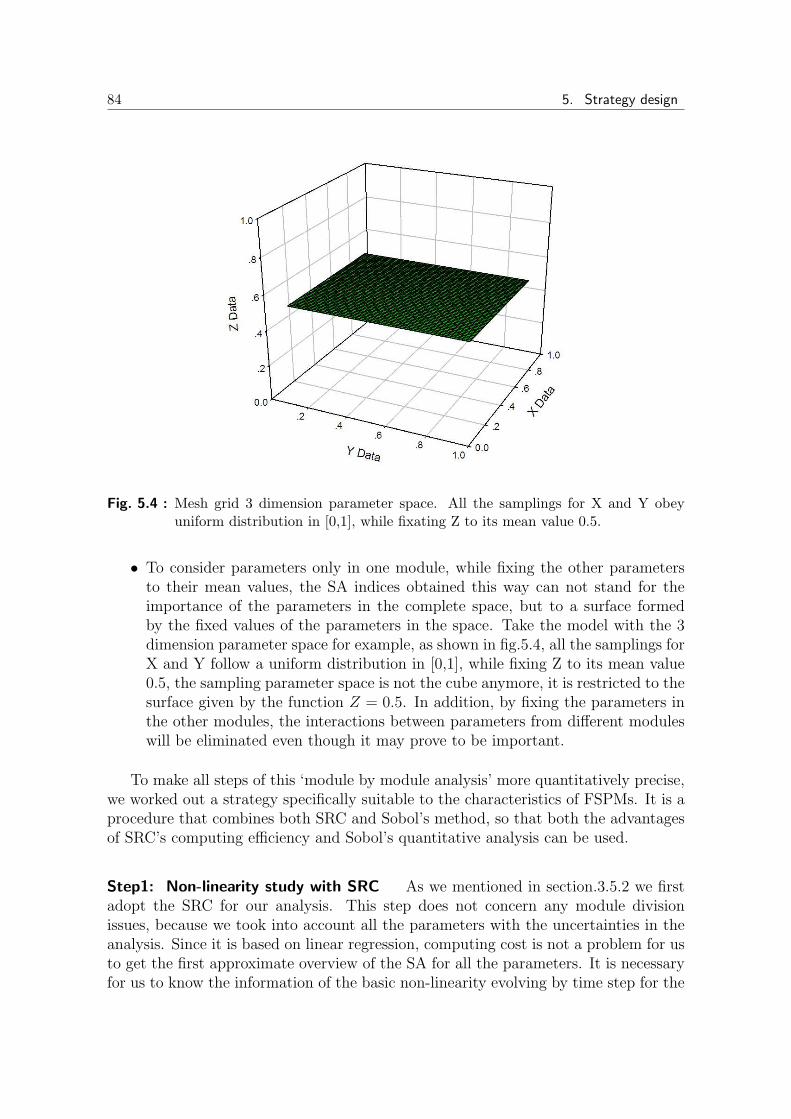
84 5. Strategy design
Fig. 5.4 : Mesh grid 3 dimension parameter space. All the samplings for X and Y obeyuniform distribution in [0,1], while fixating Z to its mean value 0.5.
• To consider parameters only in one module, while fixing the other parametersto their mean values, the SA indices obtained this way can not stand for theimportance of the parameters in the complete space, but to a surface formedby the fixed values of the parameters in the space. Take the model with the 3dimension parameter space for example, as shown in fig.5.4, all the samplings forX and Y follow a uniform distribution in [0,1], while fixing Z to its mean value0.5, the sampling parameter space is not the cube anymore, it is restricted to thesurface given by the function Z = 0.5. In addition, by fixing the parameters inthe other modules, the interactions between parameters from different moduleswill be eliminated even though it may prove to be important.
To make all steps of this ‘module by module analysis’ more quantitatively precise,we worked out a strategy specifically suitable to the characteristics of FSPMs. It is aprocedure that combines both SRC and Sobol’s method, so that both the advantagesof SRC’s computing efficiency and Sobol’s quantitative analysis can be used.
Step1: Non-linearity study with SRC As we mentioned in section.3.5.2 we firstadopt the SRC for our analysis. This step does not concern any module divisionissues, because we took into account all the parameters with the uncertainties in theanalysis. Since it is based on linear regression, computing cost is not a problem for usto get the first approximate overview of the SA for all the parameters. It is necessaryfor us to know the information of the basic non-linearity evolving by time step for the

5.3. A methodology for complex biophysical models 85
model, so that we can make an analysis decision qualified by the SRC result for thenext step. And it also helps for checking the basic ranking of the parameters. ThoughSRC does not necessarily give out the precisely ‘correct’ ranking of the parametersespecially for the system with low linearity, normally the first overview given by SRCcould be a general background information for the model.
Step2: Group analysis Our objective at this step is to compute the sensitivityindices of the total set of parameters corresponding to each module of the model. Firstwe need to make a partition of the parameters with uncertainty, so that each subsetin the partition corresponds to one biological function module of our model. Then wecompute the group indices: Sg
Ωi, ST g
Ωi, Sg
Ωijand the difference ST g
Ωi−Sg
Ωias defined in
section.3.5.2. As far as numerical computing is concerned, we use the similar matrixdefinition from section.4.1.3, except when we configure the matrix U ′
N×k and W ′N×k,
we exchange the corresponding multi-columns of WN×k and UN×k with the columnidentity of i1, i2, · · · , is, where the set of parameter identities i1, i2, · · · , is includesall the parameters belong to the module under analysis. We rewrite the matrix here:
UN×k =
x1(1) · · · xi(1) · · · xk(1)
x1(2) · · · xi(2) · · · xk(2)
.... . .
...x1(N) · · · xi(N) · · · xk(N)
,
WN×k=
x1(N+1) · · · xi(N+1) · · · xk(N+1)
x1(N+2) · · · xi(N+2) · · · xk(N+2)
.... . .
...x1(2N) · · · xi(2N) · · · xk(2N)
,
U ′N×k=
x1(1) · · · xi(N+1)1
xi(N+1)2
· · · xi(N+1)s
· · · xk(1)
x1(2) · · · xi(N+2)1
xi(N+2)2
· · · xi(N+2)s
· · · xk(2)
.... . .
...x1(N) · · · x
i(2N)1
xi(2N)2
· · · xi(2N)s
· · · xk(N)
,
W ′N×k=
x1(N+1) · · · xi(1)1
xi(1)2
· · · xi(1)s
· · · xk(N+1)
x1(N+2) · · · xi(2)1
xi(2)2
· · · xi(2)s
· · · xk(N+2)
.... . .
...x1(2N) · · · x
i(N)1
xi(N)2
· · · xi(N)s
· · · xk(2N)
.
Based on those four matrices and the method in section.4.1.3, we obtained the SgΩi,
ST gΩi
for each module and SgΩij
for each pair of modules. To distinguish from thesensitivity index of one parameter, we use a superscript ‘g’ to identify the index ofone group (one module) in this step. The computing cost for this step is not so heavybecause there are 5 modules which is much fewer than the number of parameters,with the sampling number N , the model evaluations we need here is 2N(k + 1) withk = 5. There are several small steps that relate to how to use the different SA indexgenerated by Sobol’s method to complete our analysis aims:
• Ranking module’s importance given by SgΩi. Different function modules may

86 5. Strategy design
dominate different main biological processes at different stages. This groupanalysis can help us to know the main biological process in plant growth stages.By this step, the general scheme of the sensitivity distribution among modulesis given. It is necessary to know the percentage of the first order sensitivity eachmodule takes from the whole model, because it is the background informationof the next step which provids us a quantitative clue for screening parameters.
• Identifying the intermodule interactions by computing the difference betweenST g
Ωiand Sg
Ωifor each module. It helps us to locate where the main interactions
exist, and to which extend a module can be studied independently from theother modules.
• Identifying the interactions from pairs of modules by SgΩij
. It is the specifiedinformation about the interactions inter-modules, so that it indicate us the in-teractions between biological processes.
Step3: Internal module analysis The main aim of this step is to identify themost sensitive parameters in each specific module quantitatively. On one hand weneed to consider each module separately, on the other hand, it is necessary for us tokeep one common analysis framework for all the modules, so that the quantitativecomparison can be possible between modules. So here we choose to make the analysiswith the same sampling points in the same sampling space to make the variance foreach module analysis to be the same. We stick to the improved Sobol’s mentioned insection.4.1.3 to make the analysis. We rewrite the four matrices used here to makethe basis of the two analysis basis clear:
UN×k =
x1(1) · · · xi(1) · · · xk(1)
x1(2) · · · xi(2) · · · xk(2)
.... . .
...x1(N) · · · xi(N) · · · xk(N)
WN×k=
x1(N+1) · · · xi(N+1) · · · xk(N+1)
x1(N+2) · · · xi(N+2) · · · xk(N+2)
.... . .
...x1(2N) · · · xi(2N) · · · xk(2N)
U ′N×k=
x1(1) · · · xi(N+1)m
· · · xk(1)
x1(2) · · · xi(N+2)m
· · · xk(2)
.... . .
...x1(N) · · · x
i(2N)m
· · · xk(N)
W ′N×k=
x1(N+1) · · · xi(1)m
· · · xk(N+1)
x1(N+2) · · · xi(2)m
· · · xk(N+2)
.... . .
...x1(2N) · · · x
i(N)m
· · · xk(2N)
In matrices U ′N×k and W ′
N×k, the parameter identity im means any item in the param-eters’ identity set i1, i2, · · · , is corresponding to the module we focus on. So actually

5.3. A methodology for complex biophysical models 87
for each module analysis, we used the same sampling and re-sampling matrix: UN×k
and WN×k, in this case, the output variance would be the same for all the modules,and the sum of the variance from each module would be equal to the one obtained forthe Sobol’s analysis for the overall model based on the same UN×k and WN×k.
One side advantage is that every module analysis shares the same 2N model eval-uations of UN×k and WN×k, and we simply add the model evaluations for their re-spective U ′
N×k and W ′N×k. For example, if we have r modules, and k1, k2, · · · , kr
are the numbers of parameters for each module, k1 + k2 + · · · + kr = k, k is thetotal number of parameters with uncertainty for the computed model. Using theimproved Sobol’s method in section.4.1.3, if we use the strategy in [Ruget et al.,2002], the computing cost would be 2N(k1 + 1) + 2N(k2 + 1) + · · · + 2N(kr + 1) =2N(k1+k2+ · · ·+kr)+2Nr = 2N(K+r), instead in our strategy, the computing costwould be 2N +2Nk1 +2Nk2 + · · ·+2Nkr = 2N(1+ k1 + k2 + · · ·+ kr) = 2N(K +1),it can save 2N(r − 1) model evaluations, the most important point is that it keepsall the independent module analysis being comparable by keeping them in the sameparameter space.
In fact the computing cost for module by module analysis in our strategy is thesame if we make the analysis of the overall model. So why do not we just do theoverall model analysis? Why bother to do this ‘module by module analysis’? Firstlyin [Cariboni et al., 2007], the author pointed out that the choice of most suitabletechnique for sensitivity analysis depends on the number of factors of the model and onthe CPU time required to run it. As we cut the whole set of factors into several groupsfor the model, for each module when we do the SA, the number of factors is moreappropriate for variance based technique which Sobol’s method belongs to. Secondlyit helps to get the analysis objectives more clearly, especially with the complex modelwith large number of parameters. And indeed for the computing cost, to computeseparately module by module or all modules together have the same cost. But bycombining the result of module by module analysis and group analysis, we can save alot of higher order SA index computing cost.
• In section.3.5.2, we have mentioned that the total sensitivity index STi is usedfor screening parameters: when STi ≈ 0 parameter Xi can be screened from theparameters with uncertainty, which means that the variance of this ith parameterbrings for the output can be ignored. So the module by module analysis in thisstep, we first check the index STi to screen the ignorable parameters in eachmodule. Based on this strategy, the different indices obtained in the differentmodules can be compared together. Then STi is the quantitative standard topick the most important parameters from each module.
• The comparable results of all the modules provide a quantitative standard togive the percentage of the variance explained by the selected parameters moreprecisely.
• Comprehensively consider the result in step 2 ‘group analysis’: if we computethe sum of each Si from step3 for the parameters in the module, and get the

88 5. Strategy design
Fig. 5.5 : STgΩi
for one module decomposition scheme. a.The sum of all the Si for theparameters from one module in Step 3, b.Sg
Ωifor the module minus a, intra-
module interactions from step 2, c.ST gΩi
minus SgΩi
for one module, inter-moduleinteractions in step 2
difference of it with the SgΩi
(the first order sensitivity of each parameter plusthe interactions between them within the module), for the corresponding modulewe will get the inner module interactions, which means the interactions betweenthe parameters only in the module. Moreover as we mentioned in step 2, thedifference between ST g
Ωiand Sg
Ωifor one module stands for the interactions of the
module to the others. These three parts: a. The sum of each Si from step3 forthe module, b. Sg
Ωifor the module minus a, c. ST g
Ωiminus Sg
Ωifor one module,
composite the ST gΩi
of one module as shown in fig.5.5.
Step4: Overall model analysis To make a complete sensitivity analysis with theselected parameters by the steps before. It is a ‘loop’ back to the general SA practicesteps we presented in section.3.6, except that the decision for the input factors hasbeen made.
5.4 Processing for functional output case
As we mentioned before, functional-structural plant models are dynamic models andthe output of interest evolve with time. Screening methods in sensitivity analysis gen-erally consider the case that the output is scalar. Although SA could be performedseparately at each time step for FSPMs, in the case of dynamic crop models, simu-lations are usually computed at a daily time step and the sequential implementationof global sensitivity analysis at each simulation date can result in several hundreds ofsensitivity indices, with one index per parameter per simulation date. It is not easyto identify the most important parameters based on such a large number of values.Moreover, this technique has the disadvantage of introducing a high level of redun-dancy because of the strong correlations between responses from one time step to thenext one. Likewise, intuitively, to screen one parameter, the requirement should bethat the sensitivity response curve is always near zero at all time steps, which is rarelythe case in our analysis. We therefore devise a methodology to deal with the screeningof the parameters in this dynamic context.

5.4. Processing for functional output case 89
Fig. 5.6 : NEMA: Si for 35 parameters in module dry mass fluxes (DMflux), with outputof total green area (AreaGreenTotal).
We use here a unitary concept based on the processing of averaging across time.Some parameters may have the biggest sensitivity indices at some stages for whichthe output variance is negligible. For this reason, with an averaging process, we weighthe sensitivity indices with the output variance at time t. In this way, we select theparameters that not only have the most important sensitivity at certain time steps,but also indicate the duration of this effect. We show a result for one module in NEMAmodel as example, see fig.5.6 and fig.5.7. There are 35 curves of parameter indicesin fig.5.6, and few are close to zero through the whole time period, but if we checkthe output variance through time, we will see that until thermal time 450 Cd, thetotal variance is very small, which means that the parameters dominating this periodshould be considered differently from the one dominating the period afterwards.
As such, we define a unitary index for each curve describing the first order andtotal order sensitivity averaging through time, and we call it ‘Time Generalized Index(TGI)’ for parameter with identity i:
TGISi =
∑T
t=1 V (Y (t))Si(t)∑T
t=1 V (Y (t))(5.1)
TGISTi =
∑T
t=1 V (Y (t))STi(t)∑T
t=1 V (Y (t))(5.2)
T is the total number of time steps, V (Y (t)) means the output variance at timestep t, Si(t) and STi(t) means the sensitivity indices evolving with time t.

90 5. Strategy design
Fig. 5.7 : NEMA: Total variance of output, for 35 parameters in module dry mass fluxes(DMflux), with output of total green area (AreaGreenTotal).
TGISi and TGISTi are convex combinations of Si(t) (1 ≤ t ≤ T ) so that the sameproperties as classical Si remain the same. For example, if the model is linear, for allthe parameters: ∑
i
TGISi = 1 (5.3)
TGISTi − TGISi =
∑T
t=1 V (Y (t))∑T
t=1 V (Y (t))(STi(t)− Si(t)) (5.4)
so it is characteristic of the total level of interaction for parameters.
The TGI helps us to simplify the screening processing, and at the same time,consider the evolution of the index with time, in order to guarantee that the generalizedindex we get can reflect the overall effect of the index on the output.
There has been other works that dealt with this issue. In [Ruget et al., 2002], theauthor calculated the average slope of the curve representing the output variable inrelation to the modified input parameters. In [Campbell et al., 2006], the author useda principal component analysis of output temporal curves, then compute sensitivityindices of each input on each principal component coefficient; in [Lamboni et al.,2011] they developed the multivariate global sensitivity analysis method. It allows toaggregate the different sensitivity indices of the principal component coefficients ina unique index, called the generalized sensitivity index. Each generalized sensitivityindex explains the influence of the corresponding input on the overall output curvevariability. A comparison with these methods is currently under study.

5.5. Concluding remarks and discussions 91
5.5 Concluding remarks and discussions
The objective of this study is to explore how global sensitivity analysis (SA) can helpthe design of complex models in two aspects:
• To choose proper sensitivity analysis method to fulfill different aims.
• To combine more than one SA method in order to make best use of each method’sadvantages and to make them be complementary to each other.
For the first aspect, we specially presented the SRC method and non-linearityassessment to investigate the intrinsic non-linearity of the model and of its dynamicevolution throughout plant growth, thus to study model behavior and properties, tounderline the occurrence of particular biological phenomena and hopefully, to improvethe statistical analysis when confronting models to experimental data.
For the second aspect, we developed a methodology for complex biophysical mod-els: module by module analysis inspired by [Ruget et al., 2002]. In contrast withprevious types of module by module analysis, we proposed a more reliable and effec-tive strategy of use:
• First, linearity analysis gives us the non-linearity stage information of the over-all model. This preliminary information is also useful to adapt the followingstrategy accordingly.
• Second, group analysis provides the evolution of module importance SgΩi, and
help us check inter-module interactions by ST gΩi
− SgΩi
and SgΩij
.
• Thirdly, based on the same sampling points, we run the SA module by module,in order to provide index STi of each parameter for screening. It is the basicindex for screening procedure but not the only standard. The question of howmany parameters should be selected is decided by comprehensively consideringthe results of the first and second steps. Moreover, by analyzing the compo-sition of ST g
Ωi, we get to know the intra-module and inter-module interaction
quantitatively.
• Finally, we run the SA for the overall model with the parameters selected moduleby module and check the parameter sensitivity indices for the overall model.
Conducted simulations using Sobol’s method and an efficient computation tech-nique derived from [Wu et al., 2011] will be presented in Chapter.7, and several outputsof interest are considered specially for NEMA to check how parameter effects changewith the the outputs of interest.
Moreover, since we consider a dynamic system, the evolution of the sensitivityindices is computed. And when it is related to parameter screening, we proposed

92 5. Strategy design
a time averaging index called TGI to reduce the time dimension of the sensitivityindices. Though it has not been strictly proven to be valid, it worked very well forour application. Still it is interesting to try the method in [Campbell et al., 2006] and[Lamboni et al., 2011] based on principal component analysis to see which method ismore effective and reliable.
Other methods of SA for screening for complex models can also be used, like Morris.There are references using the combination of Morris method and Sobol’s method forthe analysis of complex models. Though improved by [Campolongo and Braddock,1999] and [Cropp and Braddock, 2002], Morris method can only compute indices up tosecond order and there are two indices for one parameter: µ which assesses the overallinfluence of the factor on the output and σ which estimate the ensemble of the factor’shigher order effect [Campolongo et al., 2007]. Though it has the advantage that itcan get the coarse screening conclusion with a lower cost of model evaluations, thetwo indices for one parameter make it not so convenient to draw overall conclusions.Since the computing efficiency problem of Sobol’s method got improved the estimatorand hopefully by parallel computing, the Sobol’s method remains the most interestingfor us. That is the reason why we tried to devise a strategy to make full use of itsadvantage like STi, that can help to avoid higher order index computing and to getthe interaction information for parameters. If we can get over the problem of time-consuming model evaluation, the real convenience of Sobol’s method especially forquantitative analysis is obvious. In some situation, it might however be necessary toresort to Morris method.
What we have devised here is our practice for FSPM. It would be interesting tostudy how this method can be generalized to other types of complex systems, likeindustrial ones [Zio, 2009].

6. SOFTWARE PLATFORM: PYGMALION
6.1 Background and objectives
In the plant growth modelling community, many models have been developed fol-lowing different formalisms to understand plant growth and physiology. Several plantmodelling platforms have been proposed with the objective to ease the development ofmethods, with bricks (organogenesis, radiosity module to compute light interception,graphical tools, etc.) that can be combined.
• L-studio [Federl and Prusinkiewicz, 1999] and GroIMP [Hemmerling et al., 2008]offer integrated environment to develop new models: based on sophisticated for-malisms and providing the 3D-geometric classes for modelling and visualization.
• OpenAlea [Pradal et al., 2008] is an open source project for plant research. Itis developed with Python libraries and tools in plant architecture modelling.OpenAlea includes modules to analyse, visualize and model the functioning andgrowth of plant architecture.
These platforms allow the simulation of models but do not provide enough statis-tical tools for their analysis and evaluation, thought GroIMP does provide a range ofbasic statistical tools applicable to simulated and imported measured structures stillit does not have the tools for sensitivity analysis. On the other hand, there are alsoa lot of excellent platforms for sensitivity analysis of generic models like R packageFME [Team, 2009], Open TURNS [Andrianov et al., 2007], SimLab [Saltelli et al.,2004], etc.
The R package ‘Sensitivity’ implements sensitivity analysis methods: linear andmonotonic sensitivity analysis (SRC, PCC, SRRC, PRCC), the screening methodof Morris, and non-linear global sensitivity analysis (the Sobol indices, the FASTmethod). The functions of this package generate the design of experiments (depend-ing on the method of analysis) and compute the sensitivity indices based on the modelinputs and outputs. All sensitivity indices can be estimated with the bootstrap tech-nique which allows to estimate the bias, and basic bootstrap confidence intervals. Textand graphical outputs display the results of the analysis. 1.
1 http://cran.r-project.org/web/packages/sensitivity/index.html

94 6. Software platform: PyGMAlion
Open TURNS 2 is a Unix/Linux software, for Treatment of Uncertainty, Risk’NStatistics in a structured industrial approach. It has three main components :a scien-tific C++ library including an internal data model and algorithms dedicated to thetreatment of uncertainty; an independent application with a graphical user interface;a python module with high level operators in the probabilistic and statistical field.The targeted users are here research centers and the academic community.
SimLab 3 is a didactical software designed for Monte Carlo based uncertainty andsensitivity analysis. It is a professional tool for model developers to learn and useglobal uncertainty and sensitivity analysis techniques. Especially SimLab 3 supportsa set of coding environments such as C, C++, Matlab and Fortran.
The softwares for plant growth mostly focus on the implementation and develop-ment of plant growth modelling, but rarely on tools for model evaluation, especially forsensitivity analysis. The mentioned platforms for sensitivity analysis are not specifi-cally designed for plant or biological models.
Digiplant [Cournede et al., 2006; Cournede et al., 2011] is a first step towardsintegrating the plant growth models development and model evaluation with para-metric identification on real experimental data. It is a quite flexible and efficient tool.It has been used for parameter estimation of maize, sugar beet, sunflower, tomato,grapevine, rice, etc. It provides powerful estimation tools, but has strong limitationssince it is restricted to the GreenLab model.
An objective of the Digiplante team is to develop models of plant growth in in-teraction with the environment, to improve their predictive capacity, and to comparedifferent models. Thus, it is of great interest to integrate the models within a gen-eral platform providing the evaluation and analysis tools. On the platform, the usersdevelop models in the specific language grammar in order to plug them into the simula-tion kernel: all mathematical tools relating to model design like parameter estimation,sensitivity and uncertainty analysis can be shared for every model. PyGMAlion (Aplatform for ”Plant Growth Models’ Analysis and Identification”) is developed basedon this objective.
6.2 PyGMAlion
We recall here the steps of model design as detailed in section.2.2:
1. The conceptual model (mental work): identifying a system, state variables, in-puts; writing the different state equations involving model parameters
2 http://www.openturns.org/3 Simlab (2011) Software package for uncertainty and sensitivity analysis. Joint Research Centre
of the European Commission. Downloadable for free at: http://simlab.jrc.ec.europa.eu

6.3. Implementation in PyGMAlion 95
2. Numerical implementation: giving values to inputs, parameters and runningmodel simulations
3. Mathematical analysis: behavior, limits, stability; parametric sensitivity analy-sis
4. Parameter identification and model evaluation: ‘fitting’ experimental data; es-timate the model parameters from experimental data; estimate uncertainty ofthe estimated parameters; predictive capacity
5. Model comparison and model selection: computing some information criteria tocompare models
PyGMAlion is a C++ template based framework which embeds the routines for:
• Numerical implementation of models
• Parameter estimation
• Sensitivity and uncertainty analysis
• Model comparison and selection
Thus PyGMAlion is a platform that concerns most steps of the modelling process.For modelling methodology study, the different mathematic tools can be reused underthe same implementation scheme for different models. From a methodology point ofview, it can be figured out whether the algorithm can be applied to all types of modelsor must be adapted for some models with special characteristics. From a modellingpoint of view, the integration of the same methodology with different models makes itpossible to compare their performances in order to evaluate how well the models canachieve our modelling aims like predictive capacity, or the robustness.
6.3 Implementation in PyGMAlion
For plant growth models, we often describe the model as discrete dynamic systems orwith discretized processes of a continuous dynamic system:
Xn+1 = Fn(Xn, Un, P ) (6.1)
In which: Xn is the vector of state variables (e.g. in GreenLab it stands for massesof plant components), Fn gives the biophysical laws (e.g. the biomass production anddistribution of the organs, the photosynthesis formalism, etc.); P stands for the modelparameters which are often of genetic origin; Un is the control variables, which areoften environmental conditions like soil water and nitrogen contents, temperature, etc.
In PyGMAlion, a model is implemented as a Class Template Reference:

96 6. Software platform: PyGMAlion
PGMA::Model <StateClass , ParameterClass , EnvironmentClass >
which means that to define a model, you “simply” need:
• to define the 3 classes StateClass, ParameterClass, EnvironmentClass
• to implement a state function describing how to compute X(n + 1) from X(n)as in eqn.6.1
We provide a simple example for an equation of the Lotka-Volterra family todemonstrate how to implement a model in PyGMAlion. The Lotka-Volterra equa-tions, also known as the predator-prey equations, are a pair of first order, non-linear,differential equations frequently used to describe the dynamics of biological systemsin which two species interact, a predator and its prey. They evolve in time accordingto the pair of equations:
X(n+ 1) = X(n) + (aX(n)− bX(n)Y (n))E (6.2)
Y (n+ 1) = Y (n)− (cY (n) + dX(n)Y (n))E (6.3)
where X is population of preys, Y is the population of predators, n is the time step,a, b, c, d are the parameters representing the interaction of the two species, and E isecological environmental factor.
StateClass:
struct LVState
double X;
double Y;
LVState ()
X = 1.0;
Y = 1.0;
ParameterClass:
struct LVParameters
double a;
double b;
double c;
double d;
LVParameters ()

6.3. Implementation in PyGMAlion 97
a = 0.1;
b = 0.02;
c = 0.15;
d = 0.03;
EnvironmentClass:
struct LVEnvironment
double E;
LVEnvironment ()
E = 1.0;
State function (the body of model):
class LVModel: public PGMA::Model <LVState , LVParameters ,
LVEnvironment >
LVModel ();
LVState * nextState(PGMA::StateList <LVState > & list ,
const LVParameters & p, const LVEnvironment &env)
const LVState & Xn(list.last());
LVState * Xnplus1 = new LVState;
Xnplus1 ->X = (p.a+1)*Xn.X*env.E - p.b*Xn.X*Xn.Y*
env.E;
Xnplus1 ->Y = (-p.c+1)*Xn.Y*env.E + p.d*Xn.X*Xn.Y*
env.E;
return Xnplus1;
;
;
Beside State, Parameters, Environment, and Model, there exist two other fun-damental objects: Observer and ObservationList. Observer is a mechanism to savevalues or function of State variables during a Simulation. Observer will only be trig-gered thanks to a Timeline. ObservationList can be understood as a Database inwhich we will save these informations.
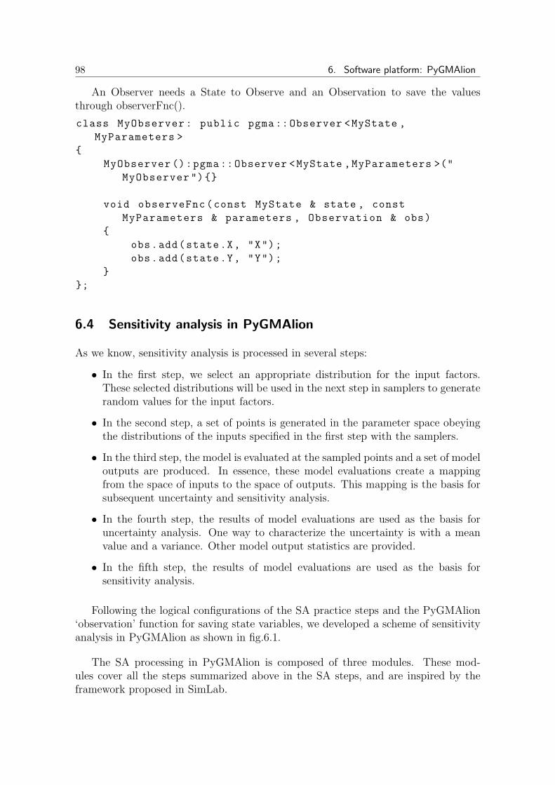
98 6. Software platform: PyGMAlion
An Observer needs a State to Observe and an Observation to save the valuesthrough observerFnc().
class MyObserver: public pgma::Observer <MyState ,
MyParameters >
MyObserver ():pgma::Observer <MyState ,MyParameters >("
MyObserver ")
void observeFnc(const MyState & state , const
MyParameters & parameters , Observation & obs)
obs.add(state.X, "X");
obs.add(state.Y, "Y");
;
6.4 Sensitivity analysis in PyGMAlion
As we know, sensitivity analysis is processed in several steps:
• In the first step, we select an appropriate distribution for the input factors.These selected distributions will be used in the next step in samplers to generaterandom values for the input factors.
• In the second step, a set of points is generated in the parameter space obeyingthe distributions of the inputs specified in the first step with the samplers.
• In the third step, the model is evaluated at the sampled points and a set of modeloutputs are produced. In essence, these model evaluations create a mappingfrom the space of inputs to the space of outputs. This mapping is the basis forsubsequent uncertainty and sensitivity analysis.
• In the fourth step, the results of model evaluations are used as the basis foruncertainty analysis. One way to characterize the uncertainty is with a meanvalue and a variance. Other model output statistics are provided.
• In the fifth step, the results of model evaluations are used as the basis forsensitivity analysis.
Following the logical configurations of the SA practice steps and the PyGMAlion‘observation’ function for saving state variables, we developed a scheme of sensitivityanalysis in PyGMAlion as shown in fig.6.1.
The SA processing in PyGMAlion is composed of three modules. These mod-ules cover all the steps summarized above in the SA steps, and are inspired by theframework proposed in SimLab.

6.4. Sensitivity analysis in PyGMAlion 99
Fig. 6.1 : PyGMAlion: Sensitivity analysis configuration
• The Pre-Processor module mainly works with samplers. It is in charge of thefirst and second steps. Most of the samplers come from Boost 4, the standardC++ library. But when special samplers are needed like Morris sampling, weimplement the samplers within PyGMAlion and add them to the function li-brary.
• The Model Execution module accomplishes the third step with the simulationkernel of PyGMAlion.
• The Post-Processor module carries out the fourth and fifth steps. Differentsensitivity index estimators are implemented in this module. Notice that bothinputs and outputs are saved in a data file: the input sampling point are savedas parameter files, and the outputs are saved in observation list files for thechosen observation variables of the model as a function of time. So that for theusers, the change of the analysis objective regarding the output of interest onlyleads to one command of observation function. It is not necessary to obtain themodel evaluations again.
So far the SA module in PyGMAlion contains SRC, Sobol’s method and Morrismethod to fulfill the SA requirements of models with different complexity. The SRCfunction generate the SRC index of each model factor and the non-linearity assessmentof the model by giving the determination coefficient R2. The Morris method is forthe qualitative analysis to screen factors. As for the Sobol’s method, we have imple-mented the classical Sobol’s method [Sobol, 1993], the H-S Sobol’s method [Hommaand Saltelli, 1996] [Saltelli, 2002] and the new Sobol’s proposed [Wu et al., 2011] inthis thesis. Test cases of the methods on Ishigami function and Lotka-Volterra modelare also given as examples for users. Graphical outputs are also produced to illustratethe results of the analysis.
4 http://www.boost.org/

100 6. Software platform: PyGMAlion

Part III
APPLICATIONS AND SIMULATIONS


7. METHODOLOGY PRACTICE:APPLICATION TO FSPMS
In the previous part, we discussed two important issues of SA for FSPMs:
• The computation issue for which we proposed an effective computational methodto evaluate Sobol’s indices and deduced the Monte Carlo simulation error esti-mation to a good control of the estimation accuracy.
• The strategy design for which we discussed the non-linearity assessment fromSRC method and ‘module by module analysis’ that analyzes the model by func-tional modules and comprehensively use diverse sensitivity methods to combinedifferent indices to avoid unnecessary high order index computing but still getthe decomposition of the portions of higher order interaction.
In this chapter, we will present the result of the application of these methodologiesto the three FSPMs with different levels of complexity introduced in section.2.4, andinfer in each case what information can be drawn from this analysis.
7.1 GreenLab maize
We first practice local SA method and its normalized version, then SRC, lastly Sobol’smethod. Our objective is to study the interest of global sensitivity analysis and its lastdevelopments for the GreenLab model, and more generally for a better understandingof source-sink dynamics and internal driving forces during plant growth.
7.1.1 Local sensitivity analysis and its normalized version
The time evolution of the biomass allocated to each type of organ qo(i) (with o = b:leaf blade; o = s: sheath; o = e: internode; o = f : cob; o = m: tassel) for the meanvalues of uncertain input factors is given in fig.7.1.
We perform the local sensitivity analysis and its normalized version (presented ineqn.3.4 and eqn.3.5) respectively to the output variables q(i) (biomass production atgrowth cycle i). The results are shown in fig.7.2.

104 7. Methodology practice: application to FSPMs
Fig. 7.1 : GreenLab Maize: biomass allocated to the different types of organs at each GC
We used numerical simulation to get the derivatives of output q(i). There are twoways to compute the standard deviations σ
Y: the first one is through Monte Carlo
simulation, which we used and is more reliable but with heavy computing cost. Toavoid this shortcoming, another possibility is to use the following approximation:
(σY)2 ∼=
∑
i
(σXi)2(∂Y
∂Xi
)2
(7.1)
Such an approximation is justified when the system is highly linear, which we willevaluate in the following section.
In fig.7.2, we see the advantage of the normalized version. The pure local SA onlyreveals the importance of µ. As for Sp, we can not even pick it out from other factorsin the pure local analysis, but with the normalized one, the great contribution of Sp ismore clearly demonstrated from about GC 12 to the end of plant growth. The basicknowledge we get from this local analysis is that the factor µ contributes the most tothe variance of biomass generation from the beginning to the end.
Note that the point at which we calculate the derivatives is important, it could benot reliable for systems with parameter-to-output curve with many apices: the valuesat these special points are not representative of the whole information of sensitivityfor this parameter. The results could be misleading, and we may miss the importantdetails of the system. Therefore more reliable methods will be applied in the nextsection.

7.1. GreenLab maize 105
(a)
(b)
Fig. 7.2 : (a). Pure local sensitivity of q with respect to the factors listed in table.2.1 asfunctions of the growth cycle (absolute values). (b). Normalized local sensitivityof qt with respect to the factors listed in table.2.1 (absolute values). Y stands forq(i) and X for the respective factors.
7.1.2 Standardized Regression coefficients
We perform a Standardized Regression method (see section.3.5.2) for the biomass pro-duction q across time with respect to all the parameters usually obtained by estimation

106 7. Methodology practice: application to FSPMs
from experimental data in GreenLab. The input factorsXi being the parameters listedin table.2.1 and the output function Y being the biomass production at a given GC,we make a linear regression according to eqn.3.6 and eqn.3.7.
The SRC indices for each parameter evolving with time are shown in fig.7.3. Thesum of SRC indices for all the parameters at each time step
∑(γ
Xi)2 and model
determination coefficient R2 are shown in fig.7.4. In Table.7.1, we present the SRCindices for all the parameters and R2 at the classical time steps which stand fordifferent growth stage for maize.
Note that the SRCs results in fig.7.3 are really close to the squared normalizedlocal measures, which is not a coincidence: for the linear system, the two should beequal. Fig.7.4 shows a very high R2,(most of the time above 0.98) proving that theSRCs indices are reliable here. The regression analysis could be used as a preliminarystep in SA to save computing time before we really do some more detailed analysis.
The crucial importance of the Radiation Use Efficiency µ is demonstrated (SRCalways above 0.6). It shows that a special care should be taken in its determination,including complementary experiments. The change of light interception can bringgreat variance for biomass production. Sp is the parameter that relates to compe-tition between plants: at the beginning when blade and sheath are forming and thecompetition for the light has not start yet, the density does not bring so much vari-ance. But at the 11th GC when the whole plant is grown and the fruit (cob for maize)appears, competition becomes dramatical and keeps increasing to the end. Alloca-tion to blades (characterized by αb and βb ) keeps a relative high importance, in thecontrast Pm keeps low. Note that for Pf which relates to the cob sink strength, theranking raises at the last stage of the whole plant growth.
Tab. 7.1 : GreenLab maize: SRC index of all the parameters and R2 at selected typical GCthat can stand for growth stages
Si of qt 1th 5th 11th 19th 30th
αb 0.0797 0.0928 0.0335 0.0017 0.0205βb 0.0062 0.0251 0.0156 0.0015 0.0117αs 0.1571 0.1997 0.0736 0.0013 0.0001βs 0.0040 0.0220 0.0135 0.0002 0.0000Ps 0.0011 0.0118 0.0178 0.0010 0.0018αe 0.0000 0.0015 0.0039 0.0000 0.0000βe 0.0000 0.0001 0.0009 0.0001 0.0000Pe 0.0000 0.0001 0.0041 0.0017 0.0044αf 0.0000 0.0000 0.0000 0.0004 0.0115βf 0.0000 0.0000 0.0000 0.0003 0.0095Pf 0.0000 0.0000 0.0000 0.0003 0.0927Pm 0.0000 0.0000 0.0000 0.0000 0.0000µ 0.6972 0.6315 0.8150 0.9778 0.8463
R2 0.9453 0.9845 0.9778 0.9863 0.9983

7.1. GreenLab maize 107
Fig. 7.3 : GreenLab maize:SRCs for the outputs q as functions of the growth cycle.
Fig. 7.4 : GreenLab maize:∑
(γXi)2 and R2
Y for the output q
7.1.3 Variance decomposition-based sensitivity measure: Sobol’smethod
The results of Sobol’s method are similar to those of local and SRC methods due tothe high linearity of the system: the parameters Sp and µ take as much as 75%∼98%of the sum for first-order index and the whole first-order sensitivity index contribute

108 7. Methodology practice: application to FSPMs
Fig. 7.5 : GreenLab model for maize:Si and STi for parameter µ
to 93%∼99% of the system variance. We computed Sobol’s first order index Si andtotal order index STi. The difference between the two indices can show whether theinteraction of this parameter to others contributes significantly to the variance of themodel output. From this point, we can still get that for the most important parameterµ, the first order SA index can totally stand for its sensitivity to the model, which isshown in fig.7.5.
So as one alternative parameter space, we fixed Sp and µ to their mean values. Infig.7.6, we show the two linearity indexes of the system, along with the summation of allSi. We note that the trends of the three curves agree with each other. The summationof Si is also characteristic of the system linearity. Actually it can be explained by thedefinition of Si: the closer to 1 the sum of the first-order indexes is in eqn.3.16, themore mutually independent the factors are, and the more linear the system is. In thenew parameter space without Sp and µ, the system linearity is weaker, especially from10th GC to 23th GC, which is the most non-linear stage of the growth, correspondingto abrupt changes in the allocation dynamics due to cob appearance. Since parametricestimation for GreenLab relies on multi-stage observations, it seems important not tomiss this crucial period in the experimental data collection.
The first order Sobol’s indices of the new set of parameters are illustrated in fig.7.7.Note that without the variance contributed by Sp and µ, αs and αb play the mostimportant roles in the system during the first 20 GCs. Afterwards the sensitivityto αf becomes the biggest until the 30th GC, after which the sensitivity to Pf risesdrastically while the sensitivities to all the other parameters drop. This trend can beexplained by analyzing maize functioning. At the beginning of maize growth, beforethe fruit appears, the factors that control the competition for biomass acquisition must

7.1. GreenLab maize 109
Fig. 7.6 : GreenLab maize: The three kinds of linearity indexes with parameter space of Spand µ fixed
play an important role, and the foliage is also privileged in the early stages of growth.It explains why the sensitivities to αs and αb are the most important ones. Theycorrespond to the parameters driving the initial form of the sink variation functionsof sheaths and blades. After the fruit (cob) appearance, it begins to attract biomass.The influence of αf (that is to say the parameter driving the initial form of the cob sinkfunction) gets bigger. But its value remains relatively low because during this timeperiod, the biomass demand of the other organs is still high. So the whole variance ofthe system output tends to be shared more uniformly during this stage between mostparameters. Towards the end of the growth, the majority of biomass production isallocated to the cob and the sensitivity to Pf increases drastically.
One thing we are more interested in is the interaction information that SA canbring us to know more about the source-sink dynamics and internal driving forcesduring plant growth. So Si and STi are compared to see if interactions exist. Takeαb for example in fig.7.8: we can see that the interaction for this parameter is activeduring the most dynamic growth duration: cob generation and internode expansion.
One more interesting point is that as we explore all the second-order Sobol’s in-dices, we found that most of the interactions concentrate between αb and the others,in which the interaction between αb and αs outmatches by far the others, see fig.7.9.
If we suppose that model parameterization can be linked to plant genes as illus-trated by [Letort et al., 2008b], the understanding of parameter interaction may beinteresting for genetic improvement. FSPM parameters may be linked to plant genes,and thus may help breeders to design ideotypes. If a parameter has little interactionwith others (like Pf ), we can directly concentrate on this trait to improve plant per-
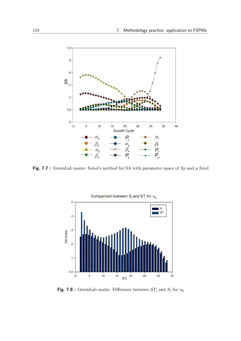
110 7. Methodology practice: application to FSPMs
Fig. 7.7 : GreenLab maize: Sobol’s method for SA with parameter space of Sp and µ fixed
Fig. 7.8 : GreenLab maize: Difference between STi and Si for αb

7.1. GreenLab maize 111
Fig. 7.9 : GreenLab maize: Interactions between αb and the other parameters
formance. If the interaction is strong, like for αb (cf fig.7.9, the interaction between αb
and αs being the most important), it is more complex. If the parameters are stronglygenetically related (determination by the same genes, which for αb, αs is probable sincethey are both characteristic of leaf geometry), the model parameterization should beimproved to take into account this fundamental interaction. If they are not geneticallyrelated, breeding strategy should rely on multi-dimensional optimization to handle theinteracting processes [Qi et al., 2010].
7.1.4 Discussion
The most important parameters for plant growth model of maize are µ (energeticefficiency) and Sp(characteristic surface related to competition between plants), whichrepresent from 75% to 98% of the first-order sensitivity index. During the process ofparameter estimation from experimental data, there is not usually a direct convergenceto the proper set of parameters because of the non-convexity of the generalized least-square function used as fitting criteria. Moreover, it was shown that the confidenceinterval on the estimated parameters might be improved by fixing some parameters[Guo et al., 2006], [Lamboni et al., 2011]. The sensitivity analysis gives us hints onhow to improve the calibration process for Maize: first fix all parameters to reasonablevalues from literature, then find estimates of µ and Sp, then find simultaneouslynew estimates for the set of αo parameters together with µ and Sp, and finally findsimultaneously new estimates for the set of sink parameters Po, together with theset of αo parameters and µ and Sp. The sensitivity analysis indicates that fixing βo
parameters is reasonable since their influence is limited.

112 7. Methodology practice: application to FSPMs
Fig. 7.10 : Poplar tree: Oscillation of the ratio of available biomass to organs’ demand(Q/D). First the ratio increases due to an increase in biomass production ata constant level of demand. When its value exceeds a threshold, new organsappear, which leads to an increase in plant demand and hence a decrease ofthe ratio. The ratio falls below the threshold, reducing the appearance of neworgans, and a decrease in the demand and so on.
7.2 Poplar tree model with retroaction of functioning onorganogenesis
In fig.7.10, is shown the evolution of the ratio of biomass production to organs’ de-mand, which is the key variable controlling tree organogenesis in the GreenLab modelof tree growth. The sensitivity analysis method was applied to the tree annual biomassproduction computed with eqn.2.7. As mentioned in [Wu and Cournede, 2009], lin-earity index is firstly checked before starting global SA. The linearity index is shownin fig.7.12. The initial states show the high linearity indices, but it decreases rapidlywith the increasing influence of the trophic competition on organogenesis, particularlythe appearance of the first branch at growth cycle 5. At this stage, the biomass pro-duction is low, because of the small number of leaves (fig. 7.11) induced by a lowerratio of biomass to demand(fig.7.10). The sensitivity index of the model for parameterµ follows the pattern of biomass production (fig.7.13).
Due to the exponential negative function, the biomass production is very sensitiveto changes in total leaf surface area when this one is small, but on the contrary, thereis a value beyond which an increase in leaf surface area will induce a very little increasein biomass production. As the leaf surface area depends on the number of organs, thebiomass production alternates between the phase close to saturation and the linearphase. In the linear phase, the model is more sensitive to the parameter Sp. On the

7.2. Poplar tree model 113
Fig. 7.11 : Poplar tree: Number of phytomers of physiological age 4. Their number dependson the ratio of available biomass to demand.
Fig. 7.12 : Poplar tree: Evolution of linearity index

114 7. Methodology practice: application to FSPMs
Fig. 7.13 : Poplar tree: Sensitivity indexes for all the model parameters
contrary, in the saturation phase, the model is more sensitive to the parameter µ asillustrated by fig.7.13.
These two parameters are the most important ones regarding biomass production.As in the study of GreenLab maize, we exclude these two parameters to get closerinsight in the other parameters driving biomass allocation - sink strengths - thatimpact plant production through the computation of leaf surface area (eqn.2.8), asshown in fig.7.14. During the youth of the tree, the trunk starts growing and no branchappears due to the low value of the ratio of biomass to demand. At this point, themodel is mainly sensitive to the parameters of phytomers of physiological age 1 ((SB)0and (SI)0 in fig.7.14. Then, the ratio of available biomass to demand increases fast,and several branches appear together. The phytomers of physiological age 4 are themost numerous in the tree as they correspond to the twigs. Their number increasestill time step 15 and then oscillates (fig.7.11), with a period corresponding to that ofthe ratio of biomass to demand (fig.7.10). Hence, the model output is sensitive totheir sink strengths ((SB)3, (SL)3 and (SI)3 on fig.7.14) with the same period, in thephases corresponding to high levels of Q/D, when a large number of twigs will appear.In the phase of low levels of Q/D, the most important parameter is the layer sinkfor secondary growth since it corresponds to the largest part of plant demand whenprimary growth is restricted.
We inspected 14 parameters related to tree biomass production and allocation, andfollow dynamically the sensitivity indices for 50 years. Note that the computation of

7.3. Model of C-N dynamics (NEMA) 115
Fig. 7.14 : Poplar tree: Sensitivity indices when fixing µ and Sp
such a long period of growth remains quite reasonable for the GreenLab model thanksto the structural factorization described in [Cournede et al., 2006]. The test casechosen corresponds to a specific model showing alternating patterns in growth phasesresulting from the complex interactions between functioning and organogenesis. Thesensitivity analysis offered interesting insight in the understanding of this interaction.Moreover, by using variance-based techniques, an analyst is capable not only of ob-taining the parameter contribution to the output variance but also of gaining insightson the model structure by using moment-independent indicators [Borgonovo, 2006].Such method provides insights on the influence of the input uncertainty on the outputdistribution [Borgonovo, 2007]. So it would be interesting for our future work to gaininsight about the output distribution (in our tree modelling case, for the variablesdescribing tree height and diameter for example). It should open a new way to deeperstudies on more complex functional-structural plant models.
7.3 Model of C-N dynamics (NEMA)
Basic biological modules are identified: namely in our test case Carbon distribution(DMflux), Nitrogen distribution (Nflux), Carbon acquisition via photosynthesis (Pho-tosynthesis), Nitrogen acquisition by roots (RootNuptake), Senescence (TissueDeath).
Several outputs of interest are considered for both intra-module and inter-moduleanalysis: a) total green area of the plant (AreaGreenTotal), b) total dry mass pro-duction of the plant (Production), c) dry mass of the grains (DMgrains), d) nitrogen

116 7. Methodology practice: application to FSPMs
mass of the grains (Ngrains) and e) root nitrogen uptake (RootNuptake). Moreover,the evolution of the sensitivity indices are computed for a better investigation of thedynamics of plant growth. When we aim at screening parameters, we consider the TGImentioned in section.5.4. The full model involves around 80 parameters. Full modeldescription can be found in [Bertheloot et al., 2011a]. We used the parameterizationof [Bertheloot et al., 2011b].
We use subscriptions to identify the factors for different plant organs as follows: gfor Grain, r for Root, La for Lamina, Sh for Sheath, In for Internode, Pe for Peduncle,Ch for Chaff.
As shown in tab.7.2, we present the result summary of our analysis following thestrategy design mentioned in section.5.3. We will present the result according to thedifferent outputs first, then we will make a comparison to see the common pointsand differences. Some steps are skipped due to the intermediate conclusions reached,for example, by the linearity analysis at the first step, we may be able to skip theinteraction analysis, either for the group analysis or for the overall model analysisbased on selected parameters.
Tab. 7.2 : NEMA: List of tables and figure describing the results of SA. Five main outputsconsidered, a) AreaGreenTotal, b) Production, c) DMgrains, d) Ngrains and e)RootNuptake, so each output was checked separately. The mark ‘-’ means thecorresponding step was skipped for the output.
a b c d e
Linearity fig.7.15 fig.7.21 fig.7.27 fig.7.30 fig.7.36
GroupSgΩi
fig.7.16 fig.7.22 fig.7.28 fig.7.31 fig.7.37
STgΩi
− SgΩi
fig.7.17 fig.7.23 - fig.7.32 fig.7.38
SgΩij
fig.7.18 fig.7.24 - fig.7.33 fig.7.39
Intra moduleTGISi, TGISTi
tab.7.3,7.4,7.5,tab.7.12,7.13 tab.7.14,7.15 tab.7.16,7.17 tab.7.21,7.22
7.6,7.7,7.8TGIS
gΩi
−∑
TGISi tab.7.9 - - tab.7.18 tab.7.23
Inter module TGISTgΩi
− TGISgΩi
tab.7.10 - - tab.7.19 tab.7.24
Overall modelSi fig.7.19 fig.7.25 fig.7.29 fig.7.34 fig.7.40
STi − Si fig.7.20 fig.7.26 - fig.7.35 fig.7.41Sij tab.7.11 - - tab.7.20 -
7.3.1 Output AreaGreenTotal
As we mentioned in section.5.3, we first applied SRC to check the linearity informationevolving with time as in fig.7.15. Between 374 Cd and 531 Cd, there is one valleyfor the linearity, during which the lowest linearity appears at 417 Cd to the linearityof 0.48. Such a period in which a strong non-linearity occurs may be characteristic ofvery specific biological phenomena during plant growth and of high level of interactions

7.3. Model of C-N dynamics (NEMA) 117
Fig. 7.15 : NEMA: Linearity: Output AreaGreenTotal, the turn point of linearity starts at374 Cd and ends at 531 Cd, the lowest linearity appears at 417 Cd.
between parameters, either known by the modeler or unknown, in which case theyshould probably be investigated more.
We then check the result of group analysis for each module, as shown in fig.7.16,fig.7.17 and fig.7.18. Fig.7.16 shows the evolution of the first order group index Sg
Ωiand
we observe a change in importance ranks of modules around 411 Cd. For ST gΩi
− SgΩi
in fig.7.17 and SgΩij
in fig.7.18, which stand for the inter-module interactions, the peaksof most of the curves overlap also around 411 Cd, which is coincides with the lowestlinearity of the model.
Our analysis points out this important stage and guides us for the parameterselection procedure in the module by module analysis part. After the parameterselection we can see that the lowest sum of first order Si in fig.7.19 and highest valueof STi − Si in fig.7.20 still appear at the same stage. After the parameter selectionstep, it is important to check if the simplified analysis keeps the same attribute suchas non-linearity period. Moreover, it also helps us focus on the Sij matrix at thistypical time point to know the parameter interaction attribute as shown in tab.7.11.
From fig.7.16, we can see that the first order sensitivity mainly goes to moduleDMfluxes and Nfluxes, and for short period of the module Tissuedeath. Fig.7.17 andfig.7.18 show that the interactions between modules mainly exist for DMfluxes andNfluxes. We also noticed that for the output AreaGreenTotal, the module Photo-synthesis and RootNuptake contribute little to the variance of the output from thebeginning to the end. Moreover, the inter-module interactions ST g
Ωi− Sg
Ωifor the two
modules are also very low at all stages. This information leads us to screen the param-eters for output AreaGreenTotal. Thus we do not need to consider the uncertainty

118 7. Methodology practice: application to FSPMs
Fig. 7.16 : NEMA: SgΩi: Output AreaGreenTotal, module Nfluxes and Tissuedeath domi-
nate the first period between 131 Cd and 411.15 Cd, the turning point of theSgΩi
for the modules’ ranking change is at 411.15 Cd, afterwards, the importanceof module DMfluxes increases dramatically, and on the contrary the indices ofNfluxes and Tissuedeath start to decrease. So module DMfulxes is the most im-portant module after 411.15 Cd. Module Photosythesis and RootNuptake keeplow sensitivity to system output AreaGreenTotal from the beginning to the end.
from these parameters while performing parameter estimation and the other modeldesign steps that the number of parameters could be a bottleneck for processing.
As for the third step: internal module analysis, we list the TGI Si and TGISTi of all the parameters module by module here to present the whole parameterselection procedure. The selected parameters from the 5 modules are marked withgrey colour in the tables. From tab.7.3 to tab.7.7, all the parameters are listed bymodules, and besides the TGI Si and TGI STi, we give out the ranking of each indexintra-module and the ranking of TGI STi in the overall model. The two types ofintra-module ranking let us see the different positions of each parameter for differentindices. And based on the same sampling points in the parameter space, the indicescan be compared inter-module, so that the overall model ranking can be used here forthe main standard of selection.
We have mentioned before in the group analysis for output AreaGreenTotal thatthe parameters belonging to modules Photosynthesis and RootNuptake may be screenedbecause the Sg
Ωiand ST g
Ωi− Sg
Ωiare nearly nil all through the whole time period. It
gets validated when we check the ranking of TGI STi for the overall model analysis.The best ranking in these two modules is for parameter ωLa,2, whose index is about0.6%. Moreover, the difference between TGI STi and TGI Si is less than 0.2%, whichcan be neglected in terms of interactions. As such, we can confirm that we can screen

7.3. Model of C-N dynamics (NEMA) 119
Fig. 7.17 : NEMA: STgΩi
− SgΩi: Output AreaGreenTotal. The first peak of the curves
appears at 127 Cd, but it only lasts for several discrete time points, and thendisappears. We can consider that the appearance of the first peak comes fromthe adaptation stage from the zero output period to the beginning of response,so that the transition period is characterized by a lot of interactions but theydon not last long. The second peak of the curves appears at 411.15 Cd, whilemodule DMfluxes and Nfluxes share the same trend as the modules with thelargest inter-module interactions.
Fig. 7.18 : NEMA: SgΩij
: Output AreaGreenTotal, the peaks of the three curves appearbetween 400 Cd and 420 Cd. The interaction between module DMfluxes andNfluxes is the most important one and lasts for the longest time.

120 7. Methodology practice: application to FSPMs
the parameters of these two modules without any risk.
We stopped the selection procedure at the 12th parameter dLa. It is related to thecomputation accuracy issue. If we check the indices after the TGI STi ranking 12th,the TGI STi < 0.65%, TGI Si < 0.48% and TGI STi − Si < 0.37%. The indices onone hand are too little for us to consider, on the other hand, their values are close tothe error of computing accuracy, therefore we only selected the first 12 parameter forthe overall model analysis. In tab.7.8, we compare the effect of the analysis beforeand after the selection. We can see that after the selection, the abandoned main effectof all the parameters to the model is 1.9% which only takes about 2% of the overallmain effect 87.3%. So we can be sure that the selected parameters can represent thewhole model by most.
Tab. 7.3 : NEMA: Module:DMfluxes; Output:AreaGreenTotal
FactorTGI Si TGI STi
IndexIntra-Module
IndexIntra-Module Model
Ranking Ranking Ranking
σMg 0.012301 4 0.040917 5 7αg 0.003365 7 0.006452 9 13βg 0.000367 11 0.011586 7 9
ttMaccg 0.008182 6 0.057255 3 4
σMr 0.018347 3 0.043396 4 5αr 0.012154 5 0.030498 6 8βr 0.061913 2 0.136818 2 2
ttMaccr 0.621337 1 0.746507 1 1δMr 1.61E-05 32 0.000332 26 46σMLa 4.99E-05 24 0.000615 22 34
αLa 1.01E-05 34 8.09E-05 31 74βLa 1.8E-05 31 0.002305 13 21
ttMaccLa 9.32E-05 20 0.005109 11 16δMLa 4.28E-05 27 0.000899 19 30σMSh
9.96E-05 19 0.000634 21 33αSh 3.86E-05 29 0.000151 30 68βSh 0.000176 14 0.002018 15 25
ttMaccSh
0.001505 8 0.003112 12 20δMSh
0.000159 16 0.000343 25 44σMIn 0.000169 15 0.000784 20 31
αIn 8.35E-05 22 0.000324 27 47βIn 0.000152 17 0.001302 17 27
ttMaccIn 0.000889 9 0.002198 14 22δMIn 0.000222 13 0.001416 16 26σMPe 3.94E-05 28 3.97E-05 34 81
αPe 2.21E-05 30 5.3E-05 33 77βPe 4.84E-05 25 0.000316 28 50
ttMaccPe 0.000352 12 0.005502 10 15δMPe 9.16E-05 21 0.001274 18 28σMCh
4.31E-05 26 7.17E-05 32 75αCh 1.44E-05 33 0.000223 29 60βCh 0.000109 18 0.000403 24 41
ttMaccCh
0.000833 10 0.008561 8 11δMCh
5.75E-05 23 0.000511 23 37
As we have concluded in section.5.3 step 3 that the difference between TGISgΩi
and∑TGISi for each module stands for the intra-module interactions. And obviously,
the difference between TGIST gΩi
and TGISgΩi
means the inter-module interactions.

7.3. Model of C-N dynamics (NEMA) 121
Tab. 7.4 : NEMA: Module:Nfluxes;Output:AreaGreenTotal
FactorTGI Si TGI STi
IndexIntra-Module
IndexIntra-Module Model
Ranking Ranking Ranking
Pg 0 28 0.000216 16 61γ 0.08179 1 0.081467 1 3Pr -5.7E-10 29 0.000216 17 62δNr 1.02E-07 24 0.00017 19 65PLa 1.56E-08 27 0.000236 15 59
σNph
La0.009076 3 0.010294 3 10
δNLa 0.023419 2 0.041367 2 6kLa,1 0.000732 5 0.000516 5 36kLa,2 0.000743 4 0.003654 4 17PSh 1E-06 20 0.000157 20 66
σNph
Sh2.72E-05 11 3.61E-05 29 82
δNSh
0.000106 8 0.000127 23 69kSh,1 4.16E-06 14 0.000487 8 39kSh,2 6.47E-06 13 6.3E-05 27 76PIn 2.88E-06 16 0.000121 24 70
σNph
In3.47E-06 15 4.13E-05 28 80
δNIn 2.2E-05 12 0.00034 11 45kIn,1 6.26E-08 25 0.000195 18 63kIn,2 6.1E-07 21 0.000245 14 58PPe 5.63E-07 22 0.000358 9 43
σNph
Pe2.82E-05 10 0.0001 25 72
δNPe 0.000182 7 0.00049 6 38kPe,1 1.92E-06 18 0.000271 12 56kPe,2 1.35E-06 19 0.000151 21 67PCh 3.77E-08 26 0.000358 9 43
σNph
Ch8.89E-05 9 0.0001 25 72
δNCh
0.000493 6 0.00049 6 38kCh,1 1.99E-06 17 0.000271 12 56kCh,2 2.26E-07 23 0.000151 21 67
Tab. 7.5 : NEMA: Module:Photosynthesis;Output:AreaGreenTotal
FactorTGI Si TGI STi
IndexIntra-Module
IndexIntra-Module Model
Ranking Ranking Ranking
ǫLa 0.000158 3 0.00027 8 57ωLa,2 0.004761 1 0.00623 1 14ǫSh 5.73E-05 4 0.000322 5 49ωSh,2 3.21E-05 6 0.000378 3 42ǫIn 8.14E-07 9 0.000294 6 51ωIn,2 3.86E-07 10 0.000178 9 64ǫPe 3.25E-06 8 4.41E-05 10 79ωPe,2 3.83E-05 5 0.000324 4 48ǫCh 2.72E-05 7 0.000436 2 40ωCh,2 0.000169 2 0.00028 7 52

122 7. Methodology practice: application to FSPMs
Tab. 7.6 : NEMA: Module:RootNuptake;Output:AreaGreenTotal
FactorTGI Si TGI STi
IndexIntra-Module
IndexIntra-Module Model
Ranking Ranking Ranking
Ur,max 0.00134 2 0.002048 3 24kr,1 0.0003 3 0.002174 2 23kr,2 4.41E-05 4 0.000521 4 35βN 0.00169 1 0.003523 1 18βC 1.28E-05 5 0.000273 5 55
Tab. 7.7 : Module:Tissuedeath;Output:AreaGreenTotal
FactorTGI Si TGI STi
IndexIntra-Module
IndexIntra-Module Model
Ranking Ranking Ranking
dLa 0.004237 1 0.008199 1 12dSh 2.36E-05 3 4.96E-05 4 78dIn 5.01E-06 5 2.12E-05 5 83dPe 2.31E-05 4 0.000276 3 54dCh 4.89E-05 2 0.000648 2 32
Tab. 7.8 : NEMA: Overall parameter selection analysis;Output:AreaGreenTotal
∑TGISi
∑SelectedTGISi Difference
DMfluxes 0.7433 0.735434 0.007866Nfluxes 0.116733 0.114285 0.002448
Photosynthesis 0.005248 0 0.005248RootNuptake 0.003386 0 0.003386Tissuedeath 0.004338 0.004237 0.000101Overall model 0.873005 0.853955 0.019049

7.3. Model of C-N dynamics (NEMA) 123
Table.7.9 shows the decomposition for the intra-module part. Generally, most intra-module interactions exist in module DMfluxes, which is as high as 8.75% in TGI.And the total intra-module interactions for all the five modules is 8.79%. Table.7.10shows the decomposition for the inter-module part. Corresponding to the conclusionwe drew from fig.7.17, most of the inter-module interaction comes between moduleDMfluxes and Nfluxes.
Tab. 7.9 : NEMA: Intra-Module Interaction analysis;Output:AreaGreenTotal
TGISgΩi
∑TGISi Intra-Module Interaction
DMfluxes 0.830802 0.7433 0.087502Nfluxes 0.117132 0.116733 0.000399
Photosynthesis 0.00531 0.005248 6.18E-05RootNuptake 0.003411 0.003386 2.47E-05Tissuedeath 0.004348 0.004338 1.04E-05Overall model 0.961002 0.873005 0.087997
Tab. 7.10 : NEMA: Inter-Module Interaction; Output:AreaGreenTotal
TGISgΩi
TGISTgΩi
Inter-Module Interaction
DMfluxes 0.830802 0.874785 0.043983Nfluxes 0.117132 0.15515 0.038019
Photosynthesis 0.00531 0.005408 9.8E-05RootNuptake 0.003411 0.003518 0.000108Tissuedeath 0.004348 0.004679 0.000331
After we decided the set of selected parameters, we run the Sobol’s method with therelatively small number of parameters to evaluate the overall parameter sensitivity.Fig.7.19 shows the Si and fig.7.20 shows the STi − Si for the selected parameters.Factor γ from module Nfluxes which stands for the relative rate of potential grain Nfilling during cell division and factor ttMacc
r from module DMfluxes which stands forthe duration during which roots can accumulate dry mass are the two most activefactors for the model while output AreaGreenTotal is considered.
For the main effect Si, these two factors share the same shape at the first stagebefore the time point 411.15 Cd with the lowest sum of Si or linearity. Afterwards γreaches a peak at around 543 Cd and then decrease little by little while ttMacc
r keepsincreasing quasi linearly and surpasses γ at around the peak point of γ.
For the interaction distribution presented by fig.7.20, most of the interaction peaksappear in the period between 374 Cd and 531 Cd, which corresponds to the non-linearity stage we found in the step 1 linearity analysis. As such, we pick the timepoint 411.15 Cd that proves to be the most important time point (for all the importanttransit and interactions, etc). To locate the interactions between parameters at thismost non-linear and interaction-active stage, we present the Sij matrix as in tab.7.11.
As shown in the table, factor γ is the only one that has relative high interactionswith all the other factors, like the STi − Si curve for γ (black line) in fig.7.20 reaches

124 7. Methodology practice: application to FSPMs
Fig. 7.19 : NEMA: Selected factors: Si; Output AreaGreenTotal; the lowest sum of Si ofall the selected factors appears at 411.15 Cd, which means around this point,the higher order sensitivity should take more part of the system variance.
its maximum at this point. Besides, factor ttMaccr also has interactions with σ
Nph
La ,δNLa, dLa which we can not ignore. The interactions stand for the main part of inter-
module interactions between module DMfluxes (ttMaccr ) and module Nfluxes (σ
Nph
La ,δNLa), between module DMfluxes (ttMacc
r ) and module Tissuedeath (dLa).
Among all these factors that have interactions with γ, σMr has the strongest in-
teraction 10.97% with γ. Another typical example is dLa, though the total rankingof dLa is the last among the selected factors and the absolute value of its TGI Si
is only 0.004, but it still has 12.31% totally of interactions at 411.15 Cd when wedo the overall model analysis with the selected factors. We can see that it has evenhigher interactions at 374 Cd in fig.7.20. Thanks to the comprehensive considerationof group analysis and module by module analysis before, we can have an appropriatestandard to decide how many factors should be selected for the overall model analysisin order not to miss such important interactions when the main effect of certain factoris low but the interaction is strong.
To demonstrate the strategy for the module by module analysis specifically, as anexample, we have presented the related indices of all the parameters with uncertaintyfor the NEMA model in this section. In the next sections, for the other model outputof interest, we use the same procedure of parameters selection that we have illustratedin detail here, so we only list the indices for the finally selected factors, and focus onthe main features for the specified output.

7.3.
Model
ofC-N
dynam
ics(N
EMA)
125
Tab. 7.11 : NEMA: Sij for selected factors at thermal time after flowering 411.15 Cd, output AreaGreenTotal
γ σMg βg ttMacc
g σMr αr βr ttMacc
r σNph
LaδNLa dLa ttMacc
Ch
γ - 0.027509 0.047476 0.038851 0.10968 0.046097 0.056311 0.047124 0.042893 0.01245 0.055861 0.032027σMg 0.027509 - 0.000967 0.0008 0.003352 7.95E-05 0.003306 -0.00043 0.002496 0.003398 0.000969 0.000381βg 0.047476 0.000967 - -0.00086 -0.00011 -0.00169 -0.00492 -0.00062 0.004646 0.009388 0.003912 3.77E-05
ttMaccg 0.038851 0.0008 -0.00086 - -0.00044 -0.00185 -0.00333 0.001642 0.003269 0.003101 0.001038 -0.00013
σMr 0.10968 0.003352 -0.00011 -0.00044 - 0.001966 5.91E-05 0.001801 0.000651 0.002221 0.005045 0.000459αr 0.046097 7.95E-05 -0.00169 -0.00185 0.001966 - -0.00212 9.12E-05 0.010585 0.017425 0.002878 -0.00038βr 0.056311 0.003306 -0.00492 -0.00333 5.91E-05 -0.00212 - 0.004816 0.007596 0.008951 0.005149 0.003311
ttMaccr 0.047124 -0.00043 -0.00062 0.001642 0.001801 9.12E-05 0.004816 - 0.031849 0.054932 0.024656 0.012335
σNph
La0.042893 0.002496 0.004646 0.003269 0.000651 0.010585 0.007596 0.031849 - 0.000103 0.011705 0.001646
δNLa 0.01245 0.003398 0.009388 0.003101 0.002221 0.017425 0.008951 0.054932 0.000103 - 0.01029 0.000257dLa 0.055861 0.000969 0.003912 0.001038 0.005045 0.002878 0.005149 0.024656 0.011705 0.01029 - 0.001625
ttMaccCh
0.032027 0.000381 3.77E-05 -0.00013 0.000459 -0.00038 0.003311 0.012335 0.001646 0.000257 0.001625 -∑j Sij 0.516279 0.042822 0.058221 0.042092 0.124683 0.073079 0.079125 0.178195 0.117438 0.122515 0.123128 0.051574

126 7. Methodology practice: application to FSPMs
Fig. 7.20 : NEMA: Selected factors: STi − Si; Output AreaGreenTotal; the peaks of mostof the curves appear at the period between 375 Cd and 411.15 Cd.

7.3. Model of C-N dynamics (NEMA) 127
7.3.2 Output Production
As for the output Production, the linearity shown in fig.7.21 keeps a relatively highvalue above 0.86. So things are more or less simplified here, but since it is not typicallyquasi-linear (> 0.95) for nearly half of the whole period, to be cautious we still keepthe interaction checking between modules in the group analysis as in fig.7.23 andfig.7.24, and fig.7.26.
The main information given by fig.7.22 is that the first order sensitivity is mainlyshared by modules Photosynthesis, Nfluxes and DMfluxes in order. Furthermore,there is little effect from module RootNuptake and Tissuedeath, likewise for the inter-module interactions. The inter-module interactions only concentrate between modulesDMfluxes and Nfluxes as shown in fig.7.23 and fig.7.24. Combining the informationwe got from the group analysis with the STi we get from the intra-module analysisin our strategy, 12 factors among 83 total for the model were selected as shown intab.7.12. The distribution is 8 factors from DMfluxes, 3 from Nfluxes and 1 fromPhotosynthesis. In tab.7.13, we can see that the screening processing for the modelhas ignored 1.29% of the main effect from 84.8%, which is a very safe amount toguarrantee the reliability of the results afterwards.
As we can see in fig.7.25, in the first period before 465 Cd, ωLa,2 (the only factor
selected from module Photosynthesis), δNLa and σNph
La (the 2 out of 3 factors frommodule Nfluxes) take most portion of the uncertainty. For the last period, ttMacc
r frommodule DMfluxes and γ from module Nfluxes take the role in change. It correspondsto what was observed regarding module indices in the group analysis, as shown infig.7.22. Again, basic features are kept after the parameter selection.
For interactions between selected factors, the 3 ones γ, βr and ttMaccr were identified
for this issue as shown in fig.7.26, in which ttMaccr is responsible for most part of the
interaction.

128 7. Methodology practice: application to FSPMs
Fig. 7.21 : NEMA: Linearity: Output Production. There is a small slope between 360 Cdand 474 Cd, the drop is from 0.99 to 0.86. Before and after this slope, thereare two flat levels with the linearity around 0.99 and 0.86 respectively.
Fig. 7.22 : NEMA: SgΩi
Output Production. Module Photosynthesis ranks first from thebeginning to 165 Cd, at which point module Nfluxes surpasses it. ModuleDMfluxes starts to increase steadily at point 341 Cd with the index 0.08, afterwhich it crosses with module Photosynthesis at point 423 Cd with value 0.243and crosses with module Nfluxes at point 474 Cd with value 0.36. After thesetwo crossed points, module DMfluxes gets to dominate the model uncertainty.

7.3. Model of C-N dynamics (NEMA) 129
Fig. 7.23 : NEMA: ST gΩi
− SgΩi: Output Production. The negative values are caused by
the computing accuracy limitation. The only interaction is between modulesDMfluxes and Nfluxes. They share the same evolution. At 520 Cd, they reachthe highest value as 0.12.
Fig. 7.24 : NEMA: SgΩij
: Output Production. The peak value is 0.09 at 520 Cd.

130 7. Methodology practice: application to FSPMs
Tab. 7.12 : NEMA: Selected factors; Output:Production
FactorTGI Si TGI STi
IndexIntra-Module
IndexIntra-Module Model
Ranking Ranking Ranking
Module: DMfluxesσMg 0.010966 6 0.026162 6 9αg 0.001963 8 0.012057 8 12βg 0.001687 9 0.013025 7 11
ttMaccg 0.013809 5 0.06488 3 4
σMr 0.016135 3 0.046696 5 6αr 0.013812 4 0.051463 4 5βr 0.04353 2 0.105708 2 2
ttMaccr 0.629453 1 0.768214 1 1
Module: Nfluxesγ 0.067811 1 0.098038 1 3
σNph
La0.007753 3 0.024685 3 10
δNLa 0.017416 2 0.034581 2 8Module: PhotosynthesisωLa,2 0.010495 1 0.039516 1 7
Tab. 7.13 : NEMA: Overall parameter selection analysis;Output:Production
∑TGISi
∑SelectedTGISi Difference
DMfluxes 0.737226 0.731355 0.005871Nfluxes 0.095379 0.092979 0.002399
Photosynthesis 0.011457 0.010495 0.000962RootNuptake 0.00332 0 0.00332Tissuedeath 0.000443 0 0.000443Overall model 0.847825 0.834829 0.012996
Fig. 7.25 : NEMA: Selected factors Si; Output Production. ωLa,2, δNLa and σNph
La dominatethe model from beginning to 465 Cd. Afterwards, γ and ttMacc
r rank first, thedifference is that γ starts decreasing after a short period of increasing and ttMacc
r
keeps a steady increase.

7.3. Model of C-N dynamics (NEMA) 131
Fig. 7.26 : NEMA: Selected factors STi − Si; Output Production. The difference betweenSTi and Si concentrate only for γ, βr and ttMacc
r , which are the first 3 factorsin the overall model ranking (see tab.7.12).

132 7. Methodology practice: application to FSPMs
Fig. 7.27 : NEMA: Linearity: Output DMgrains
7.3.3 Output DMgrains
As in fig.7.27, the linearity of the model with DMgrains as the output is always above0.95, which is high enough for us to take the model as quasi-linear. So we can ignorethe interactions either between the modules or between the parameters in the analysis.So all the steps related to the interaction analysis are skipped here.
As for the group analysis in fig.7.28, we can see the module DMfluxes has theobvious priority over all the other modules all along time. Module Nfluxes and Photo-synthesis have the same trend over time. These two sets of curves go through a reversechange, from 446 Cd to 629 Cd, which is explained by fig.7.29: the transit is causedby the decrease in sensitivity of σM
g , αg from module DMfluxes and a small increaseof ωLa,2 from module Photosynthesis, δNLa from module Nfluxes. Module RootNuptakeand Tissuedeath have little effect upon the output variance.
Considering the group analysis result and the intra-module analysis, we selected12 factors out of 83 as shown in tab.7.15. Due to the high linearity of the system withoutput DMgrains, the selected factors shown in tab.7.15 have the same ranking for Si
and STi. The difference of the sensitivity indices ignored by the selection is 0.089 asshown in tab.7.15.
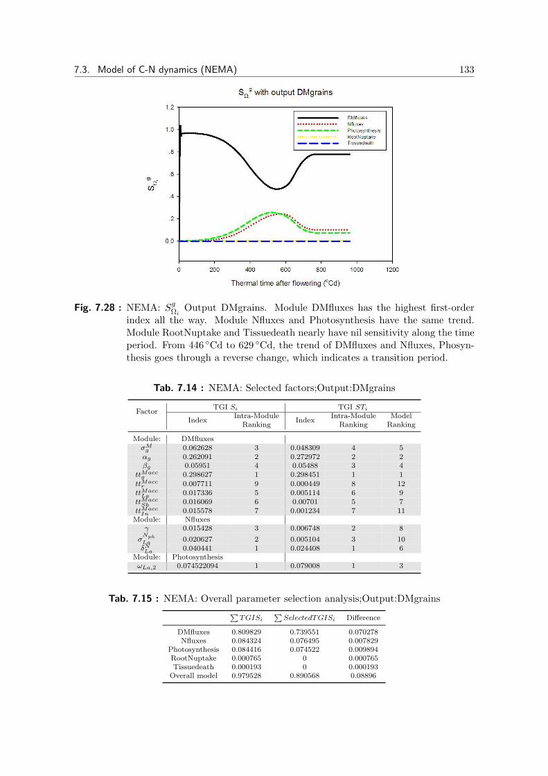
7.3. Model of C-N dynamics (NEMA) 133
Fig. 7.28 : NEMA: SgΩi
Output DMgrains. Module DMfluxes has the highest first-orderindex all the way. Module Nfluxes and Photosynthesis have the same trend.Module RootNuptake and Tissuedeath nearly have nil sensitivity along the timeperiod. From 446 Cd to 629 Cd, the trend of DMfluxes and Nfluxes, Phosyn-thesis goes through a reverse change, which indicates a transition period.
Tab. 7.14 : NEMA: Selected factors;Output:DMgrains
FactorTGI Si TGI STi
IndexIntra-Module
IndexIntra-Module Model
Ranking Ranking Ranking
Module: DMfluxesσMg 0.062628 3 0.048309 4 5αg 0.262091 2 0.272972 2 2βg 0.05951 4 0.05488 3 4
ttMaccg 0.298627 1 0.298451 1 1
ttMaccr 0.007711 9 0.000449 8 12
ttMaccLa 0.017336 5 0.005114 6 9
ttMaccSh
0.016069 6 0.00701 5 7ttMacc
In 0.015578 7 0.001234 7 11Module: Nfluxes
γ 0.015428 3 0.006748 2 8
σNph
La0.020627 2 0.005104 3 10
δNLa 0.040441 1 0.024408 1 6Module: PhotosynthesisωLa,2 0.074522094 1 0.079008 1 3
Tab. 7.15 : NEMA: Overall parameter selection analysis;Output:DMgrains
∑TGISi
∑SelectedTGISi Difference
DMfluxes 0.809829 0.739551 0.070278Nfluxes 0.084324 0.076495 0.007829
Photosynthesis 0.084416 0.074522 0.009894RootNuptake 0.000765 0 0.000765Tissuedeath 0.000193 0 0.000193Overall model 0.979528 0.890568 0.08896

134 7. Methodology practice: application to FSPMs
Fig. 7.29 : NEMA: Selected factors Si: Output DMgrains. αg starts with the first rankingwith high portion of sensitivity but decrease to nil until 549 Cd, after whichttMaccg increases until around 0.7 at the end period. The indices of Si for σ
Mg and
ωLa,2 meet at 446 Cd, and those of Si for ωLa,2 and ttMaccg meet at 629.125 Cd,
between the two points, ωLa,2 from module Photosynthesis and δNLa from moduleNfluxes rank the first two factors. It is interpreted by the transition period inmodule analysis in fig.7.28.

7.3. Model of C-N dynamics (NEMA) 135
Fig. 7.30 : NEMA: Linearity: Output Ngrains. The system is linear from the beginning to494 Cd. After a steady decrease until 748 Cd with linearity 0.78, the systembasically maintains the same linearity level though with a slight increase.
7.3.4 Output Ngrains
Shown in fig.7.30, as for the linearity when the system output is Ngrains, the model isslightly non-linear after 600 Cd. We followed the same analysis steps as when systemoutput is AreaGreenTotal.
In fig.7.31, modules DMfluxes and Nfluxes have the complementary trends for SgΩi
while the other three modules have nearly no effect. Then it is not a surprise that themain inter-module interaction goes directly between module DMfluxes and Nfluxes asshown in fig.7.32 and fig.7.33.
We follow the standard procedure for the parameter selection detailed in sec-tion.7.3.1. For the output Ngrains, the sensitivity main effect is very concentratedon 6 factors from two modules: DMfluxes and Nfluxes, as shown in tab.7.16. Fromtab.7.17, we can see that even only with 6 factors among 83 for the overall model,they have already explained the main effect 84.34% of the variance out of 86.37% forall the 83 factors, with only a loss of 2%.
A similar concentration also appears for the intra-module interaction shown intab.7.18 and the inter-module interaction shown in tab.7.19: most intra-module inter-action only exists in module DMfluxes and the inter-module interaction only happensbetween DMfluxes and Nfluxes.

136 7. Methodology practice: application to FSPMs
Fig. 7.31 : NEMA: SgΩi
Output Ngrains. Module Nfluxes has the most important effect tothe system until 685 Cd, after which DMfluxes gets more and more importanceand Nfluxes effect decreases steadily.
Fig. 7.32 : NEMA: ST gΩi
−SgΩi, Output Ngrains. It is obvious that only modules DMfluxes
and Nfluxes have interaction regarding the output Ngrains. Note that the peakalso appears at the transit point 685 Cd between Nfluxes and DMfluxes.

7.3. Model of C-N dynamics (NEMA) 137
Fig. 7.33 : NEMA: SgΩij
Output Ngrains
Tab. 7.16 : NEMA: Selected factors;Output:Ngrains
FactorTGI Si TGI STi
IndexIntra-Module
IndexIntra-Module Model
Ranking Ranking Ranking
Module: DMfluxesttMacc
g 0.004262 6 0.006578 5 6
σMr 0.014819 3 0.02549 3 4αr 0.011334 4 0.018858 4 5βr 0.035907 2 0.053437 2 3
ttMaccr 0.31217 1 0.438664 1 2
Module: Nfluxesγ 0.464929 1 0.553625 1 1
Tab. 7.17 : NEMA: Overall parameter selection analysis; Output:Ngrains
∑TGISi
∑SelectedTGISi Difference
DMfluxes 0.392619 0.378493 0.014126Nfluxes 0.467102 0.464929 0.002173
Photosynthesis 0.002535 0 0.002535RootNuptake 0.00142 0 0.00142Tissuedeath 1.18E-05 0 1.18E-05Overall model 0.863687 0.843421 0.020266
Tab. 7.18 : NEMA: Intra-Module Interaction analysis; Output:Ngrains
TGISgΩi
∑TGISi Intra-Module Interaction
DMfluxes 0.446579 0.392619 0.053961Nfluxes 0.467633 0.467102 0.000531
Photosynthesis 0.002995 0.002535 0.00046RootNuptake 0.001532 0.00142 0.000112Tissuedeath 2.02E-05 1.18E-05 8.37E-06Overall model 0.918759 0.863687 0.055072

138 7. Methodology practice: application to FSPMs
Tab. 7.19 : NEMA: Inter-Module Interaction; Output:Ngrains
TGISgΩi
TGISTgΩi
Inter-Module Interaction
DMfluxes 0.446579 0.535207 0.088628Nfluxes 0.467633 0.542965 0.075332
Photosynthesis 0.002995 0.00439 0.001396RootNuptake 0.001532 -0.00316 -0.0047Tissuedeath 2.02E-05 -0.00736 -0.00738
Fig. 7.34 : NEMA: Selected factors Si Output Ngrains. Similar transition exists betweenfactor γ from module Nfluxes and factor ttMacc
r from module DMfluxes as infig.7.31, which means that the two factors can represent most part of the variancefrom these two modules respectively.
Tab. 7.20 : NEMA: Sij for selected factors at thermal time after flowering 685 Cd, out-put Ngrains. The interaction between γ and ttMacc
r takes most part of theinteraction between parameters at this time point.
γ ttMaccg σM
r αr βr ttMaccr
γ - 0.005294 0.031051 0.003267 0.021093 0.129051ttMacc
g 0.005294 - 0.002653 -0.00193 0.001179 0.006328
σMr 0.031051 0.002653 - -0.00089 0.001278 0.009428αr 0.003267 -0.00193 -0.00089 - 0.000261 0.00506βr 0.021093 0.001179 0.001278 0.000261 - 0.011148
ttMaccr 0.129051 0.006328 0.009428 0.00506 0.011148 -
∑j Sij 0.189756 0.01352 0.043517 0.00576 0.034959 0.161015

7.3. Model of C-N dynamics (NEMA) 139
Fig. 7.35 : NEMA: Selected factors STi − Si Output Ngrains. γ and ttMaccr have the same
curve shape of the higher order interactions. At 685 Cd, besides the stronginteraction for γ and ttMacc
r , βr also cotribute around 10% to the higher ordersensitivity.

140 7. Methodology practice: application to FSPMs
Fig. 7.36 : NEMA: Linearity: Output RootNuptake. The non-linearity is very strong andpresents strong variability.
7.3.5 Output RootNuptake
Generally, the system for output RootNuptake is very non-linear and with strongvariability shown in fig.7.36. The first order sensitivity concentrates on module Root-Nuptake as for a short period at the beginning and then module DMfluxes as infig.7.37. However the interactions between modules are more complicated. By check-ing Sg
Ωiin fig.7.38 and Sg
Ωijin fig.7.39 together, two types of inter-module interactions
were identified: DMfluxes and Nfluxes, DMfluxes and Photosynthesis.
The factor selection procedure only cut 0.6% of the first order sensitivity as shownin tab.7.22, which means 16 factors out of 83 in total can reflect the main effect ofthe system when the output is RootNuptake. By analyzing the selected factors intab.7.21, intra-module interactions (mainly in DMfluxes as high as 24% when aver-aging with time) are stronger than inter-module interactions (between 0.11 and 0.14appropriately) as in tab.7.23 and tab.7.24.
In fig.7.40, we can see that parameter ttMaccr stands for most part of the main effect
of the system, but the interactions between parameters are distributed evenly for theselected factors as shown in fig.7.41. So it is necessary to check by modules for theinteractions to get more oriented precise insights.

7.3. Model of C-N dynamics (NEMA) 141
Fig. 7.37 : NEMA: SgΩi
Output RootNuptake. Module RootNuptake only dominates oneshort period at the beginning and module DMfluxes takes the most importantrole until the end. As for the main effect, module Nfluxes, Photosynthesis andTissuedeath keeps low values all the time.
Fig. 7.38 : NEMA: ST gΩi
− SgΩi
Output RootNuptake. Interactions exist among moduleDMfluxes, Nfluxes and Photosynthesis.

142 7. Methodology practice: application to FSPMs
Fig. 7.39 : NEMA: SgΩij
Output RootNuptake
Tab. 7.21 : NEMA: Selected factors;Output:RootNuptake
FactorTGI Si TGI STi
IndexIntra-Module
IndexIntra-Module Model
Ranking Ranking Ranking
Module: DMfluxesσMg 0.0082 5 0.169337 6 6αg 0.006524 7 0.089024 8 11βg 0.003358 8 0.123071 7 7
ttMaccg 0.024149 3 0.232268 3 3
σMr 0.012747 4 0.1813 5 5αr 0.007595 6 0.18315 4 4βr 0.042309 2 0.331893 2 2
ttMaccr 0.491072 1 0.857027 1 1
ttMaccLa 0.000751 10 0.070719 12 16
ttMaccSh
8.18E-05 22 0.0784 11 14ttMacc
In 0.000482 11 0.07992 10 13ttMacc
Ch0.001178 9 0.084181 9 12
Module: Nfluxesγ 0.007203 1 0.113062 1 8
σNph
La0.00126 3 0.075261 3 15
δNLa 0.002005 2 0.09054 2 10Module: PhotosynthesisωLa,2 0.001996381 1 0.101541 1 9
Tab. 7.22 : NEMA: Overall parameter selection analysis; Output:RootNuptake
∑TGISi
∑SelectedTGISi Difference
DMfluxes 0.600248 0.598448 0.0018Nfluxes 0.011304 0.010468 0.000837
Photosynthesis 0.002105 0.001996 0.000108RootNuptake 0.003351 0 0.003351Tissuedeath 7.08E-05 0 7.08E-05Overall model 0.617079 0.610912 0.006167

7.3. Model of C-N dynamics (NEMA) 143
Tab. 7.23 : NEMA: Intra-Module Interaction analysis; Output:RootNuptake
TGISgΩi
∑TGISi Intra-Module Interaction
DMfluxes 0.840487 0.600248 0.240238Nfluxes 0.01109 0.011304 -0.00021
Photosynthesis 0.003427 0.002105 0.001323RootNuptake 0.003808 0.003351 0.000457Tissuedeath 0.00013 7.08E-05 5.93E-05Overall model 0.858941 0.617079 0.241862
Tab. 7.24 : NEMA: Inter-Module Interaction; Output:RootNuptake
TGISgΩi
TGISTgΩi
Inter-Module Interaction
DMfluxes 0.840487 0.981854 0.141367Nfluxes 0.01109 0.127559 0.116469
Photosynthesis 0.003427 0.087084 0.083657RootNuptake 0.003808 0.021292 0.017484Tissuedeath 0.00013 0.009546 0.009416
Fig. 7.40 : NEMA: Selected factors Si: Output RootNuptake

144 7. Methodology practice: application to FSPMs
Fig. 7.41 : NEMA: Selected factors STi − Si: Output RootNuptake

7.3. Model of C-N dynamics (NEMA) 145
7.3.6 Comprehensive comparison
Mathematically for sensitivity analysis, the definition of one model for the analysisincludes the equations describing the phenomenon and one scalar output variable. Sowhen the outputs are different though the equations are the same for our analysis, wetake each case as different mathematical model. That’s the reason why we presentedthe results for each output in the previous sections.
Even though from a mathematical point of view the models are different, as for themodelers, we still hope that from the result of several outputs we can get a commonview for the model. So we listed the selected parameters for all the interesting outputswe have analyzed in tab.7.25 along together with their rankings corresponding to thefirst order index Si in the overall model.
From tab.7.25 we can see that though with differences, the selected factors thatcan take most portion for the variance of the system concentrate on 17 factors out of83 in total for the model. This conclusion has already helped us a lot to reduce thenumber of parameters with uncertainties when doing the parameter estimation.
What’s more, if we check the diversity in details, we can find that the distributionof the selected factors is 12 out of 34 factors for module DMfluxes, 3 out of 28 factorsfor module Nfluxes, 1 out of 5 factors for module Tissedeath, 1 out of 10 factors formodule Photosynthesis and 0 out of 5 for module RootNuptake. And as we usedSTi for the screening, when we check the Si ranking here, we can see that not allthe parameters selected are the ones with the biggest Si. For example, within the12 selected factors, βg, output AreaGreenTotal ranks 21st regarding Si . So as wementioned in section.5.3, we can not rely on selecting the factors according to Si
ranking in the intra-module analysis. The right way is to check the STi ranking onthe basis of the same sampling points for each module analysis, plus comprehensivelyconsidering the group analysis for each module.
For NEMA model itself, the most important factors set for module Nfluxes arepretty steady for all the outputs: 1) γ standing for the relative rate of potential
grain N filling during cell division, 2) σNph
La standing for relative rate of photosyntheticN synthesis associated to xylem influx for entity Lamina, 3) δNLa standing for relativedegradation rates of remobilizable N for entity Lamina, in which γ rules all the outputsand most of the time has the very high ranking. γ appears to be a crucial factor forthe general NEMA model. For the 28 factors in this module, the sensitivity is veryconcentrated on these 3 ones. However, for module DMfluxes, it is not the case.The 12 factors for DMfluxes have different rankings for different outputs. Generally,1) ttMacc
r standing for the duration during which roots can accumulate dry mass 2)ttMacc
g standing for stands for the duration during which grains can accumulate drymass, those two rank among the most important for all the 5 outputs. Secondarily,1) σM
g standing for relative sink strength of grains, 2) σMr standing for relative sink
strength of roots, 3) αr, βr standing for Beta function indices for roots, have also

146 7. Methodology practice: application to FSPMs
noticeable effect for 4 of the outputs. Compared to modules DMfluxes and Nfluxes,modules Tissuedeath and Photosynthesis tend to have specific important parametersfor different outputs, like dLa (standing for proportion of maximum specific N mass atwhich tissues die for Lamina) for output of AreaGreenTotal and ωLa,2 (standing forproportion coefficient linking photosynthesis at saturating PAR and N mass per unit)specially for output DMgrains.
If we categorize the factors in tab.7.25 by organs, we can see that in the 4 typesof parameters presented in tab.2.3 for module DMfluxes, the ones for organ grain androot tend to have significant effect for all outputs. The parameter characteristic oflamina tend to have the control for Nfluxes, Tissuedeath and Photosynthesis.
Tab. 7.25 : NEMA: Summary of selected factors’ Si ranking in overall model for differentoutputs. There are 5 main outputs we considered in the analysis, a) AreaGreen-Total, b) Production, c) DMgrains, d) Ngrains and e) RootNuptake. Factorsthat are selected for all the 5 outputs are marked in dark grey and for 4 outputsare marked in light grey. ‘-’ means the factor is not selected for output.
Si ranking a b c d e
Module:DMfluxes
σMg 6 8 4 - 5αg - 12 2 - 8βg 21 13 5 - 9
ttMaccg 9 7 1 7 3
σMr 5 5 - 4 4αr 7 6 - 5 6βr 3 3 - 3 2
ttMaccr 1 1 13 2 1
ttMaccLa - - 8 - 16
ttMaccSh
- - 9 - 32ttMacc
In - - 10 - 17ttMacc
Ch17 - - - 15
Module:Nfluxes
γ 2 2 11 1 7
σNph
La8 10 7 - 14
δNLa 4 4 6 - 10
Module:Tissuedeath
dLa 11 - - - -
Module:Photosynthesis
ωLa,2 - 9 3 - 11

7.4. Conclusions and discussion 147
7.4 Conclusions and discussion
In this chapter, we implemented the strategy developed in this thesis to 3 FSPMswith different levels of complexity, and inferred in each case what information can bedrawn from this analysis.
Firstly we practiced on a simple source-sink model of maize growth, which is usedto specifically study the process of carbon (C) allocation among expanding organsduring plant growth, with simple plant structure, multi-stage and detailed observa-tions. We first practiced local SA method and its normalized version, then SRC, lastlySobol’s method. We studied the interest of global sensitivity analysis and its latestdevelopments for the GreenLab model. SA helped us to get better understanding ofsource-sink dynamics and internal driving forces during plant growth.
Secondly we practiced on the GreenLab model of tree growth (applied to poplartree) characterized by the retroaction of plant functioning on its organogenesis, whichdescribes tree structural plasticity in response to trophic competition. We inspected 14parameters related to tree biomass production and allocation, and follow dynamicallythe sensitivity indices for 50 years. The test case chosen corresponds to a specific modelshowing alternating patterns in growth phases resulting from the complex interactionsbetween functioning and organogenesis.
Lastly we practiced on a functional-structural model, NEMA, describing C andnitrogen (N) acquisition by a wheat plant as well as C and N distributions betweenplant organs after flowering. This model is more mechanistic and more complex thanthe two previous ones. Basic biological modules are identified: namely in our test caseCarbon distribution, Nitrogen distribution, Carbon acquisition via photosynthesis,Nitrogen acquisition by roots, Senescence. Several outputs of interest are consideredfor both intra-module and inter-module analysis: a) total green area of the plant, b)total dry mass production of the plant, c) dry mass of the grains, d) Nitrogen mass ofthe grains and e) root Nitrogen uptake. Basically, for each output of interest, we did1) the non-linearity assessment, 2) the analysis of function module rankings, 3) theintra module analysis, 4) the inter module analysis, and finally 5) the overall modelanalysis based on the result of the 4 analyse before.
The real advantage of Sobol’s method was particularly illustrated for the differentsteps of our method for module by module analysis, and its application to NEMA.For the specific analysis of NEMA, an important step has not been fully completed.It corresponds to the biological diagnosis of the model. Once sensitivity analysisrevealed the importance of some very specific stage of growth, it would be interestingto really analyze from a biological point of view the processes that make these stagesof interest. From a modelling point to view, being able to show that 17 parametersout of 83 can explain most of the variance is an important step forward, particularlyfor parameterization. However, we should also question why no parameter from themodule of RootNuptake was selected: either the uncertainty of the parameters in

148 7. Methodology practice: application to FSPMs
this module was underestimated, or level of description of the model structure is notappropriate.

Part IV
CONCLUSIONS AND PERSPECTIVES


8. CONCLUSIONS AND PERSPECTIVES
8.1 Contributions
Global sensitivity analysis has a key role to play in the design and parameterizationof functional-structural plant growth models (FSPM) which combine the descriptionof plant structural development (organogenesis and geometry) and functional growth(biomass accumulation and allocation). Models of this type generally describe manyinteracting processes, count a large number of parameters, and their computationalcost can be important. The general objective of this thesis is to develop a propermethodology for the sensitivity analysis of functional structural plant models and toinvestigate how sensitivity analysis can help for the design and parameterization ofsuch models as well as providing insights for the understanding of underlying biologicalprocesses. Our contribution can be summarized as follows:
• In order to face the challenge of the computing cost and to meet the necessity ofusing Sobol’s indices for the quantitative information about sensitivity of mod-els, especially the interaction information, we improved a computing methodinspired by [Homma and Saltelli, 1996] so that the model evaluations can bemade best use of. We derived an estimator of the error of sensitivity indicesevaluation with respect to the sampling size for this generic type of computa-tional methods so that better control of the convergence of the estimations ofSobol’s indices can be achieved.
• We designed a methodology adapted to FSPMs. We first discussed the use ofnon-linearity assessment to identify the occurrence of particular biological phe-nomena, and then processed a strategy to conduct ‘module by module analysis’in order to comprehensively integrate different SA methods and indices when acomplex biophysical system characterized by the interaction of several processesdescribed by sub-models/modules is analyzed.
• We applied the developed methodology of sensitivity analysis to 3 FSPMs withdifferent levels of complexity, and inferred in each case what information canbe drawn from this analysis. Better understanding of source-sink dynamics andinternal driving forces during plant growth are achieved. Especially for NEMAmodel,‘module by module analysis’ helped to understanding the model behaviorfrom the classical simulation approach.

152 8. Conclusions and perspectives
Fig. 8.1 : Brief illustration of improved Sobol’s estimator. ‘Sobol 1993’ see [Sobol,1993],‘Homma et Saltelli’ see [Homma and Saltelli, 1996]. Matrices in the frameof the same line type are involved in one factor index estimation. y: model outputof sampling matrix, yR: model output of re-sampling matrix, y′: model outputof sampling matrix with ith column re-sampled, y′
R: model output of re-samplingmatrix with ith column re-sampled.
Computational issue
It is necessary for us to use a precise global sensitivity analysis method like Sobol’s tolocate the quantitative interaction information between parameters. However FSPMsusually have a large number of parameters and the model evaluation is computation-ally heavy, so the implementation of the SA strategy faces a great challenge regardingthe computing cost issue. It is crucial to not only devise efficient computing tech-niques, in order to make best use of model evaluations, but also to have a good errorestimation to check whether the SA computing has properly converged.
Based on the idea of ‘making best use of model evaluations’ and making thesampling-resampling processing ‘smoother’ by ‘averaging’, we proposed a new Sobol’sestimator to improve the computing efficiency and convergence of the method. For theHomma-Saltelli method, to estimate each of the k first order indices, the computingcost is N(k + 2) model runs, with N model runs for the initial sampling matrix out-put evaluation y, N model runs for the initial re-sampling matrix output evaluationyR, Nk model runs for the re-sampling matrix generated for conditional variance ofoutput y′
R. What we proposed is to add the complementary ‘sampling’ matrix y′ intothe evaluation which increases the number of sampling matrices involved for the SAindex for one factor from 3 to 4. With the 4 matrices, when the role of ‘sampling’ and‘re-sampling’ matrices change, we get two sets of SA index evaluations. As in fig.8.1,the set of matrices within real line frame and dashed line frame are two sets of SAindex evaluations. When we average the two sets of indices, since the sampling getsmore ‘balanced’, a better convergence has been achieved by the improved estimator.Plus, by adding with Nk more model runs, that is to say with the computing cost ofN(2k + 2) model runs while we make full use of the 2N samplings, two sets of SAindices estimation can be done, so that some computing cost has been saved. Thecomputing test on Ishigami function has proved to yield the better performance ofour new Sobol’s estimator.
Previous work as in [Homma and Saltelli, 1996] gave interesting result about error

8.1. Contributions 153
estimation, but the conclusions are based on some restrictive assumptions. We alsoderived for the generic type of computational methods as illustrated in fig.8.1 an errorestimation of sensitivity indices with respect to the sampling size. It is based on somerules to compute ‘the moments of functions of random variables’. It allows a detailedcontrol of the balance between accuracy and computing time and can also be used togive confidence bounds of the result.
Strategy design
A good sensitivity analysis practice does not only need well designed estimators (whichis one of the thesis objectives as recalled in the previous paragraph), but it also requiresa good understanding of the issues that can be tackled by different methods, and howthese methods can be combined to benefit from their respective advantages. Theseconsiderations underlies the strategy design for SA.
Typically to show how to make best use of SRC for FSPMs, we discussed the non-linearity assessment based on a side result of SRC: the determination coefficient R2.The knowledge of the intrinsic non-linearity of the model and of its dynamic evolutionthroughout plant growth identified by R2 proved to be useful to study model behaviorand properties, to underline the occurrence of particular biological phenomena or toimprove the statistical analysis when confronting models to experimental data.
For complex biological systems which are characterized by several interacting pro-cesses with sub-modules describing each of them, especially for some FSPMs, thestrategy design should be divided into several steps for which we choose different SAmethods to fulfill different requirements. An interesting point is the evaluation of theimportance of the ‘function’ modules of FSPMs, which means checking the sensitiv-ity effects of the groups of parameters. This is how ‘module by module’ analysis forcomplex biophysical systems is proposed.
In our ‘module by module’ analysis, the following sensitivity indices and some oftheir combinations are used. We recall the type of information the different indicesand methods provide:
• Non-linearity index from SRC: The level of non-linearity evolution of the modeland the general view of the model dynamic property.
• Sobol’s first order index Si: The main effect of factor Xi, mainly used for ‘FactorPriorization’.
• Sobol’s total order index STi: The total effect of factor Xi, mainly used for‘Factor fixing’ or screening.
• The difference between STi and Si: The sum of interactions of all orders betweenXi and the other factors.

154 8. Conclusions and perspectives
• Sobol’s second order index Sij: The interaction between factors Xi and Xj.
• First order group indices SgΩi: The main effect of the set of factors Ωi which
usually gathers the inputs of one module.
• Total order group index ST gΩi: The total effect of factor set Ωi.
• The difference between ST gΩi
and SgΩi: The sum of interactions of all orders
between factor set Ωi and the other sets.
• Second order group indices SgΩij
: The interaction between factor sets Ωi and Ωj.
The proposed strategy follows the steps:
• First, linearity analysis gives us the non-linearity stage information of the over-all model. This preliminary information is also useful to adapt the followingstrategy accordingly.
• Second, group analysis provides the evolution of module importance SgΩi, and
helps us to check inter-module interactions by ST gΩi
− SgΩi
and SgΩij
.
• Thirdly, based on the same sampling points, we run the SA module by module,in order to provide index STi of each parameter for screening. It is the basicindex for screening procedure but not the only standard. The question of howmany parameters should be selected is decided by comprehensively consideringthe results of the first and second steps. Moreover, by analyzing the compo-sition of ST g
Ωi, we get to know the intra-module and inter-module interaction
quantitatively.
• Finally, we run the SA for the overall model with the parameters selected moduleby module and check the parameter sensitivity indices for the overall model.
Analyses are conducted using Sobol’s method and the efficient computation tech-nique derived from [Saltelli, 2002], and several outputs of interest are considered spe-cially for NEMA to check how parameter effects change with the outputs of interest.
Moreover, since we consider a dynamic system, the evolution of the sensitivity in-dices is computed. When it is related to parameter screening, we use a time averagingindex called TGI to reduce the time dimension of the sensitivity indices.
SA practice for FSPMs
We implemented the strategy developed in this thesis to 3 FSPMs with differentlevels of complexity, and inferred in each case what information can be drawn fromthis analysis.

8.1. Contributions 155
1. Firstly we practiced on a simple source-sink model of maize growth, which isused to specifically study the process of carbon (C) allocation among expandingorgans during plant growth, with simple plant structure, multi-stage and detailedobservations. We first practiced local SA method and its normalized version,then SRC, lastly Sobol’s method. We studied the interest of global sensitivityanalysis and its latest developments for the GreenLab model. SA helped usto get better understanding of source-sink dynamics and internal driving forcesduring plant growth. The following conclusions can be noted:
• The most important parameters for GreenLab maize are µ (energetic ef-ficiency) and Sp (characteristic surface related to competition betweenplants). A non-linear period was identified thanks to R2 index. It indicatesa key stage in terms of biophysical processes corresponding to the transi-tion between two allocation phases: the first one corresponding mostly toleaf area increase and the second one to grain filling.
• The parametric estimation of GreenLab by model inversion relies on multi-stage observations, so the information given by the linearity analysis canbe taken advantage of. For maize, it is important to have detailed andfrequent observations between cycles 14 and 20, while the measurementscan be less frequent after cycle 20.
• The sensitivity analysis gives us hints on how to improve the calibrationprocess for maize model: first fix all parameters to reasonable values fromliterature, then find estimates of µ and Sp, then find simultaneously newestimates for the set of αo parameters together with µ and Sp, and fi-nally find simultaneously new estimates for the set of sink parameters Po,together with the set of αo parameters and µ and Sp. The sensitivity anal-ysis indicates that fixing βo parameters is reasonable since their influenceis limited.
• The interaction information given by SA enlightens the source-sink dynam-ics and internal driving forces during plant growth. Most of the interactionsconcentrate between αb and the others, in which the interaction betweenαb and αs outmatch by large.
• The understanding of parameter interaction is crucial for genetic improve-ment. FSPM parameters may be linked to plant genes, and thus may helpbreeders to design ideotypes. If a parameter has little interaction with oth-ers, we can directly concentrate on this trait for the design of ideotypes.If the interaction is strong, it is more complex. If the parameters arestrongly genetically related (determination by the same genes), the modelparameterization should be improved to take into account this fundamen-tal interaction. If they are not genetically related, breeding strategy shouldrely on multi-dimensional optimization to handle the interacting processes.
2. Secondly we practiced on the GreenLab model of tree growth (applied to poplartree) characterized by the retroaction of plant functioning on its organogenesis,

156 8. Conclusions and perspectives
which describes tree structural plasticity in response to trophic competition. Weinspected 14 parameters related to tree biomass production and allocation, andfollow dynamically the sensitivity indices for 50 years. The test case chosencorresponds to a specific model showing alternating patterns in growth phasesresulting from the complex interactions between functioning and organogenesis.The sensitivity analysis offered interesting insight in the understanding of thisinteraction:
• Due to the exponential negative function in the production function inGreenLab, the biomass production is very sensitive to changes in total leafsurface area when it is small, but on the contrary, there is a value beyondwhich an increase in leaf surface area will induce very little increase inbiomass production. In the linear phase, the model is more sensitive to theparameter Sp. On the contrary, in the saturation phase, the model is moresensitive to the parameter µ.
• In the youth stage of the tree, the trunk starts growing and no branchappear due to the low value of the ratio of biomass to demand. At thispoint, the model is mainly sensitive to the parameters of phytomers ofphysiological age 1 ((SB)0: blade sink and (SI)0:internode sink). The ratioof available biomass to demand increases fast, and several branches appeartogether. The phytomers of physiological age 4 are the more numerous inthe tree as they correspond to the twigs. Their number increases till timestep 15 and then oscillates. The model output is sensitive to their sinkstrengths ((SB)3, (SL)3 and (SI)3) with the same period.
• In the phases corresponding to high levels of Q/D, a large number ofbranches will appear. In the phase of low levels Q/D, the most impor-tant parameter is the layer sink for secondary growth since it correspondsto the largest part of plant demand when primary growth is restricted.
3. Lastly we practiced on a functional-structural model, NEMA, describing C andnitrogen (N) acquisition by a wheat plant as well as C and N distributions be-tween plant organs after flowering. This model is more mechanistic and morecomplex than the two previous ones. Basic biological modules are identified:namely in our test case Carbon distribution, Nitrogen distribution, Carbon ac-quisition via photosynthesis, Nitrogen acquisition by roots, Senescence. Severaloutputs of interest are considered for both intra-module and inter-module anal-ysis: a) total green area of the plant, b) total dry mass production of the plant,c) dry mass of the grains, d) Nitrogen mass of the grains and e) root Nitrogenuptake. Basically, for each output of interest, we did 1) the non-linearity assess-ment, 2) the analysis of function module rankings, 3) the intra module analysis,4) the inter module analysis, and finally 5) the overall model analysis based onthe result of the 4 analyse before. Some detailed conclusions can be drawn:
• The most important achievement of this practice work for NEMA is that 17factors out of 83 total can be selected as priority factors for all the 5 outputs

8.2. Discussion and perspectives 157
of interest. It is a big step towards the model simplification of NEMA andcan potentially lead to more optimized work on parameter estimation inthe next modelling step.
• Relying on selecting the factors according to Si ranking in the intra-moduleanalysis is not appropriate. The right way is to check the STi rankingon the basis of the same sampling points for each module analysis, pluscomprehensively considering the group analysis for each module.
• The most important factors for module Nfluxes are fairely steady for all theoutputs: 1) γ (relative rate of potential grain N filling during cell division),
2) σNph
La (relative rate of photosynthetic N synthesis associated to xyleminflux for entity Lamina), 3) δNLa (relative degradation rates of remobilizableN for entity Lamina), in which γ rules all the outputs and most of the timehas the very high ranking. γ appears to be a crucial factor for the generalNEMA model. For the 28 factors in this module, the sensitivity is veryconcentrated on these 3 ones.
• For module DMfluxes, the later statement is not appreciate. The 12 factorsfor DMfluxes have different rankings for different outputs. Generally, 1)ttMacc
r (the duration during which roots can accumulate dry mass) 2) ttMaccg
(the duration during which grains can accumulate dry mass), those tworank among the most important for all the 5 outputs. Secondarily, 1) σM
g
(relative sink strength of grains), 2) σMr (relative sink strength of roots), 3)
αr, βr (Beta function indices for roots), have also a noticeable effect on 4of the outputs.
• Compared to modules DMfluxes and Nfluxes, modules Tissuedeath andPhotosynthesis tend to have specific important parameters for differentoutputs, like dLa (proportion of maximum specific N mass at which tissuesdie for Lamina) for output of AreaGreenTotal and ωLa,2 (proportion co-efficient linking photosynthesis at saturating PAR and N mass per unit)specially for output DMgrains.
• If we categorize the factors by organs, for module DMfluxes, the ones fororgan grain and root tend to have a significant effect on all outputs. Theparameter characteristic of lamina tend to have the control over Nfluxes,Tissuedeath and Photosynthesis.
• The module RootNuptake has very little influence on the 5 outputs ofinterest. It questions the modelling part for this module and invites towork again on the structure and parameterization of this module.
8.2 Discussion and perspectives
Sensitivity analysis (SA) is a fundamental tool in the building, use and understandingof mathematical models [Saltelli et al., 2008]. Though we have done some work onthis topic in this thesis, a lot more is expected for us to keep improving SA’s role inFSPMs community.

158 8. Conclusions and perspectives
Evaluation of the distribution of the inputs
Most of the time, the distributions of input factors are not easy to obtain. A possiblestrategy is to perform an initial exploratory analysis with rather crude definition forthe distribution of the inputs and use sensitivity analysis to identify the most impor-tant inputs; then, resources can be concentrated on characterizing the uncertainty ofthese inputs and a second sensitivity analysis can be carried out with these improveduncertainty characterizations [Helton et al., 2006b]. In this thesis, we have imple-mented the first step. A study to explore the variability of parameters in a family ofgenotypes for the SUNFLO model [Lecoeur et al., 2011] will be implemented in ourfuture work.
Computational issue
Fighting with computation cost is a key issue in the case of a model with a huge num-ber of parameters as potentially for FSPMs. Though we have proposed an improvedSobol’s estimator to achieve better computing efficiency and convergence characteris-tics compared to its previous version, there is still room for improvement. In a recentpaper [Saltelli et al., 2010], the authors compared different types of estimators for STi,and Jansen’s estimator [Jansen, 1999] is shown to be the most efficient. It would thusbe interesting to adapt our strategy to make best use of model evaluations to otherestimators to check whether the same convergence characteristics can be obtained. Aproper sampling design is also an important aspect of computational issue. It relatesto the convergence properties of the Monte Carlo simulation [Tarantola et al., 2012].Thus it is also interesting for us to investigate which type of sampling design is themost appropriate for our SA practice in FSPM.
Parallel computing
As the main bottleneck of the computing cost is model evaluation for the outputmatrices, and model evaluations are actually independent from each other, it wouldbe interesting to use parallel computing to reduce the computing time for sensitivityanalysis. Efficient exchange of data would still be a challenge. A study on this issueis in process in the Digiplante team.
Sensitivity analysis and model selection
The estimation of the uncertain parameters from experimental data is an importantstep and model performances depend a lot on the accuracy of the parameter estima-tion ([Butterbach-Bahl et al., 2004]; [Gabrielle et al., 2006]; [Lehuger et al., 2009];[Makowski et al., 2006]). In general, it is impossible to estimate all parameters ofcomplex models simultaneously [Bechini et al., 2006]. During the process of parame-ter estimation from experimental data, there is not usually direct convergence to theproper set of parameters because of the non-convexity of the generalized least-square

8.2. Discussion and perspectives 159
function used as fitting criterion. Moreover, it was shown that the confidence inter-val on the estimated parameters might be improved by fixing some parameters [Guoet al., 2006], [Lamboni et al., 2011]. A common strategy consists in selecting a subsetof parameters to be calibrated using sensitivity analysis, and fixing the others to somenominal values ([Monod et al., 2006]; [Wallach et al., 2002]).
Parameters fixed as recommended values are treated as constants in models. There-fore the problem to choose parameters needed to be estimated turns out to be a statis-tical model selection problem in which candidate models may have different numbersof parameters. Thus, model selection procedure need to be done after processing pa-rameter estimation by the help of sensitivity analysis for ‘Factor priorization’ so thatthe model can be validated.
Sensitivity analysis with dynamic output and multi-variate outputs
Dynamic functional structural plant models frequently simulate state variables acrossdiscrete time step. The dynamic structure of these models introduces a strong tempo-ral correlation between the different model outputs. For a discrete-time model, globalsensitivity analysis methods can be applied sequentially at each simulation time step.The sequential implementation of global sensitivity analysis at each time step canresult in several hundreds of sensitivity indices, with one index per time step. It isnot easy to identify the most important parameters based on such a large number ofvalues [Campolongo et al., 2007]. In addition, there is a high level of redundancy fromthe discrete-time outputs.
Another problem is that when we analyze one model, usually, there is not only onemodel output of interest. Generally there are several variables of interest, as usually inmore general complex systems [Zio, 2003]. Therefore, one factor has several differentsensitivity indices for the different outputs. It is difficult to consider all the indicesfor all outputs for a given factor to evaluate its effect on the whole model.
We used in this thesis a unitary concept based on the averaging across time called‘Time Generalized Index (TGI)’ to resolve the problem of time dimension redundancyof the SA indices. Since the final result we obtained in NEMA is that all the analysisfor different outputs of interest underlines the important effect to a relatively similarset of factors, we did not consider a synthetic index to summarize the indices for alltypes of outputs.
In [Campbell et al., 2006], the author used a principal component analysis of out-put temporal curves, then compute sensitivity indices of each input on each principalcomponent coefficient; in [Lamboni et al., 2011] they developed the multivariate globalsensitivity analysis method. It allows to aggregate the different sensitivity indices ofthe principal component coefficients in a unique index, called the generalized sensi-tivity index. Each generalized sensitivity index synthesizes the effects of uncertain

160 8. Conclusions and perspectives
factors on all the dynamic outputs obtained from dynamic models, and thus explainsthe influence of the corresponding factor on all outputs at all time steps. It will beinteresting to use this kind of index for the analysis of a broader range of models.
Deterministic and stochastic models
All the models we considered in this thesis are deterministic models and the methodswe used are mostly appropriate for this type of model. However, in the FSPM mod-elling community, stochastic models have been widely developed in the past decades[Kang et al., 2008] [Loi and Cournede, 2008] [Pallas et al., 2011]. They also needsensitivity analysis to help for the parameter priorization or for model simplification.There are several references about this issue [Ginot et al., 2006], [Lurette et al., 2009].
Correlated input factors
Though it is not easy to know the correlation between input parameters , it may beof interest and was not considered in this thesis. In [Saltelli and Tarantola, 2002], theauthors devised a strategy for sensitivity analysis that could work for correlated inputfactors, based on the first-order and total-order indices from variance decomposition.Specially, we will use this strategy to investigate SA of plant models with uncertaininputs representing genotype parameters [Buck-Sorlin et al., 2005] in a family linkedthrough correlation matrix [Letort et al., 2008b].
Influence of the input uncertainty on the output distribution
Sensitivity analysis offers interesting insight for the understanding of the importanceranking and interactions of factors. Moreover, by using variance-based techniques, ananalyst is capable not only of obtaining the parameter contribution to the output vari-ance but also of gaining insights on the model structure by using moment-independentindicators [Borgonovo, 2006]. Such methods provide indications of the influence of theinput uncertainty on the output distribution [Borgonovo, 2007]. It would be interest-ing for our future work to gain insight about the output distribution (in our treemodelling case, for the variables describing tree height and diameter for example).
8.3 To conclude
In this thesis, we attempt to explore and demonstrate the benefit of SA to the FSPMcommunity in which we still find papers in the recent years processing SA by onlyconsidering local methods [Evers et al., 2007]. The potential use of SA in the plantmodelling process is very interesting, both in terms of model parameterization, butalso as a tool for model diagnosis. An effort to promote the recent methods andmake them easily available in the FSPM community is made through the platform

8.3. To conclude 161
PyGMAlion for plant modelling, which is now used in some other plant modellinggroups specifically for SA.

162 8. Conclusions and perspectives

APPENDIX


A. APPROXIMATION THE MOMENTS OFFUNCTIONS OF RANDOM VARIABLES
It is possible to approximate the moments of a function f of random variables X,Y using Taylor expansions, provided that f is sufficiently differentiable and that themoments of X and Y are finite [Bevington and Robinson, 2003]. Let us denote theexpectations E(X) = µX , E(Y ) = µY , and variances V (X) = σ2
X , V (Y ) = σ2Y . We
thus get the following results:
Theorem A.0.1: Suppose Z = f(X), then
E(Z) ≈ f(µX) +f ′′(µX)
2σ2X (A.1)
V (Z) ≈ [f ′(µX)σX ]2 (A.2)
Proof Make the second order Taylor expansion for Z = f(X) at the point of X = µ,get:
Z = f(X) = f(µ) + f ′(µ)(X − µ) +f ′′(µ)
2(X − µ)2 +R2(X)
where R2(X) is the remainder for the second order Taylor expansion, ignore thisremainder, then:
Z ≈ f(µ) + f ′(µ)(X − µ) +f ′′(µ)
2(X − µ)2
Add the expectation calculator to it:
E(Z) ≈ E[f(µ) + f ′(µ)(X − µ) +f ′′(µ)
2(X − µ)2]
= E[f(µ)] + E[f ′(µ)(X − µ)] + E[f ′′(µ)
2(X − µ)2]
= f(µ) + f ′(µ)E(X − µ) +f ′′(µ)
2E(X − µ)2
= f(µ) +f ′′(µ)
2σ2
Make the first order Taylor expansion for Z = f(X) at the point of X = µ, get:
Z = f(X) = f(µ) + f ′(µ)(X − µ) +R1(X)

166 A. Approximation of the moments of functions of random variables
where R1(X) is the remainder for the first order Taylor expansion, ignore this remain-der, then:
Z ≈ f(µ) + f ′(µ)(X − µ)
Add the variance calculator to it:
V (Z) ≈ V [f(µ) + f ′(µ)(X − µ)]
= V [f(µ)] + V [f ′(µ)(X − µ)]
= 0 + f ′2(µ)V (X − µ)
= f ′2(µ)V (X)
= f ′2(µ)σ2
Theorem A.0.2: suppose Z = f(X, Y ), then
E(Z) ≈ f(µX , µY ) (A.3)
+1
2fxx(µX , µY )σ
2X
+ fxy(µX , µY )cov(X, Y )
+1
2fyy(µX , µY )σ
2Y
V (Z) ≈ [fx(µX , µY )σX ]2 (A.4)
+ [fy(µX , µY )σY ]2
+ 2fx(µX , µY )fy(µX , µY )cov(X, Y )
Proof Make the second order Taylor expansion for Z = f(X, Y ) at the point of(µX , µY ), get:
Z = f(X, Y )
= f(µX , µY ) + [fx(µX , µY )(X − µX) + fy(µX , µY )(Y − µY )]
+1
2[fxx(µX , µY )(X − µX)
2 + 2fxy(µX , µY )(X − µX)(Y − µY ) + fyy(µX , µY )(Y − µY )2]
+ R2(X, Y )
where R2(X, Y ) is the remainder for the second order Taylor expansion, ignor thisremainder, add the expectation calculator to it, then:
E(Z) ≈ E[f(µX , µY )] + E[fx(µX , µY )(X − µX) + fy(µX , µY )(Y − µY )]
+1
2E[fxx(µX , µY )(X − µX)
2 + 2fxy(µX , µY )(X − µX)(Y − µY ) + fyy(µX , µY )(Y − µy)2]
= f(µX , µY ) + 0 +1
2fxx(µX , µY )E[(X − µX)
2] + fxy(µX , µY )E[(X − µX)(Y − µY )]
+1
2fyy(µX , µY )E[(Y − µy)
2]
= f(µX , µY ) +1
2fxx(µX , µY )σ
2X + fxy(µX , µY )cov(X, Y ) +
1
2fyy(µX , µY )σ
2Y

167
Make the first order Taylor expansion for Z = f(X, Y ) at the point of (µX , µY ), get:
Z = f(X, Y ) = f(µX , µY ) + fx(µX , µY )(X − µX) + fy(µX , µY )(Y − µY ) +R1(X, Y )
where R1(X, Y ) is the remainder for the first order Taylor expansion, ignor this re-mainder, add the expectation calculator to it, then:
V (Z) ≈ V [f(µX , µY ) + fx(µX , µY )(X − µX) + fy(µX , µY )(Y − µY )]
= V [fx(µX , µY )(X − µX) + fy(µX , µY )(Y − µY )]
= V [fx(µX , µY )(X − µX)] + 2E[fx(µX , µY )(X − µX)fy(µX , µY )(Y − µY )]
+ V [fy(µX , µY )(Y − µY )]
= f 2x(µX , µY )V (X − µX) + 2fx(µX , µY )fy(µX , µY )E[(X − µX)(Y − µY )]
+ f 2y (µX , µY )V (Y − µY )
= f 2x(µX , µY )σ
2X + 2fx(µX , µY )fy(µX , µY )cov(X, Y ) + f 2
y (µX , µY )σ2Y
In particular,
• if Z = X2, thenE[Z] = µ2
X + σ2X (A.5)
V [Z] ≈ 4µ2Xσ
2X (A.6)
• and if Z = X ± Y , then:
E[Z] = µX ± µY (A.7)
V [Z] = σ2X + σ2
Y ± 2cov(X, Y ) (A.8)
• and if Z = X/Y , then:
E[Z] ≈ µX
µY
− 1
µ2Y
cov(X, Y ) +µX · µY
µ4Y
· σ2Y (A.9)
V [Z] ≈ 1
µ2Y
· σ2X − 2 · µX
µ3Y
· cov(X, Y ) +µ2X
µ4Y
· σ2Y (A.10)

168 A. Approximation of the moments of functions of random variables

BIBLIOGRAPHY
M. Allen, P. Prusinkiewicz, and T. Dejong. Using L-systems for modeling source-sinkinteractions, architecture and physiology of growing trees, the L-peach model. NewPhytologist, 166:869–880, 2005.
G. Andrianov, S. Burriel, S. Cambier, A. Dutfoy, I. Dutka-Malen, E. de Rocquigny,and B. Sudret. Open turns, an open source initiative to treat uncertainties, risks’nstatistics in a structured industrial approach. In Proceedings of ESREL 2007: The18th European Safety and Reliability Conference, 2007. ESREL2007, Stavenger,Norway.
D. Barthelemy and Y. Caraglio. Plant architecture: a dynamic, multilevel and com-prehensive approach of plant form, structure and ontogeny. Annals of Botany, 99:375–407, 2007.
L. Bechini, S. Bocchi, T. Maggiore, and R. Confalonieri. Parameterization of a cropgrowth and development simulation model at sub-model components level. an exam-ple for winter wheat (triticum aestivum l.). Environmental Modelling & Software,21(7):1042 – 1054, 2006.
J. Bertheloot, P. Martre, and B. Andrieu. Dynamics of light and nitrogen distributionduring grain filling within wheat canopy. Plant Physiology, 148(3):1707–1720, 2008.
J. Bertheloot, P.-H. Cournede, and B. Andrieu. Nema, a functional-structural modelof nitrogen economy within wheat culms after flowering. i. model description. Annalsof Botany, 108(6):1085–1096, 2011a.
J. Bertheloot, Q.-L. Wu, P.-H. Cournede, and B. Andrieu. Nema, a functional-structural model of nitrogen economy within wheat culms after flowering. ii. evalu-ation and sensitivity analysis. Annals of Botany, 108(6):1097–1109, 2011b.
P.-R. Bevington and D.-K. Robinson. Data reduction and error analysis for the phys-ical sciences. Boston, MA: McGraw-Hill, 2003.
B. Blocken and C. Gualtieri. Ten iterative steps in development and evaluation ofenvironmental models. Environmental Modelling & Software, 21(5):602 – 614, 2006.
E. Borgonovo. Measuring uncertainty importance: Investigation and comparison ofalternative approaches. Risk Analysis, 26:1349–1361, 2006.

170 BIBLIOGRAPHY
E. Borgonovo. A new uncertainty importance measure. Reliability Engineering &System Safety, 92(6):771 – 784, 2007.
G. Buck-Sorlin and K. Bachmann. Simulating the morphology of barley spike pheno-types using genotype information. Agronomie, 20:691–702, 2000.
G. Buck-Sorlin, O. Kniemeyer, and W. Kurth. Barley morphology, genetics and hor-monal regulation of internode elongation modelled by a relational growth grammar.New Phytologist, 166(3):859–867, 2005.
K. Butterbach-Bahl, M. Kesik, P. Miehle, H. Papen, and C. Li. Quantifying theregional source strength of n-trace gases across agricultural and forest ecosystemswith process based models. Plant and Soil, 260:311–329, 2004.
D. Cacuci. Sensitivity and Uncertainty Analysis: Theory, volume I. Chapman & Hall,2003.
D. Cacuci, I.-B. Mihaela, and N. Michael. Sensitivity And Uncertainty Analysis:Applications to Large-Scale Systems, volume II. Chapman & Hall, 2005.
K. Campbell, M. D. McKay, and B. J. Williams. Sensitivity analysis when modeloutputs are functions. Reliability Engineering & System Safety, 91(10-11):1468–1472, 2006.
F. Campolongo and R. Braddock. The use of graph theory in the sensitivity analysisof the model output: a second order screening method. Reliability Engineering &System Safety, 64(1):1 – 12, 1999.
F. Campolongo, J. Cariboni, and A. Saltelli. An effective screening design for sensitiv-ity analysis of large models. Environmental Modelling and Software, 22:1509–1518,2007.
J. Cariboni, D. Gatelli, R. Liska, and A. Saltelli. The role of sensitivity analysis inecological modelling. Ecological modelling, 203:167–182, 2007.
M. Chelle. Phylloclimate or the climate perceived by individual plant organes: Whatis it? how to model it? what for? New Phytologist, 166(3), 2005.
P.-H. Cournede, V. Letort, A. Mathieu, M.-Z. Kang, S. Lemaire, S. Trevezas, F. Houl-lier, and P. de Reffye. Some parameter estimation issues in functional-structuralplant modelling. Mathematical Modelling of Natural Phenomena, 6(2):133–159,2011.
P.-H. Cournede, M.-Z. Kang, A. Mathieu, J.-F. Barczi, H.-P. Yan, B.-G. Hu, andP. de Reffye. Structural Factorization of Plants to Compute their Functional andArchitectural Growth. Simulation, 82(7):427–438, 2006.
R. A. Cropp and R. D. Braddock. The new morris method: an efficient second-orderscreening method. Reliability Engineering & System Safety, 78(1):77 – 83, 2002.

BIBLIOGRAPHY 171
R. Cukier, C. Fortuin, K. Shuler, A. Petschek, and J. Schaibly. Study of the sensitivityof coupled reaction systems to uncertainties in rate coefficients. J. Chem. Phys., 59(i):3873–3878, 1973.
R. Cukier, H. Levine, and K. Shuler. Study of the sensitivity of coupled reactionsystems to uncertainties in rate coefficients. J. Chem. Phys., 26(1), 1978.
P. de Reffye and B.-G. Hu. Relevant choices in botany and mathematics for buildingefficient dynamic plant growth models: the greenlab case. In B. Hu and M. Jaeger,editors, Plant Growth Models and Applications, pages 87–107. Tsinghua UniversityPress and Springer, 2003.
P. De Reffye, F. Fourcaud, T.and Blaise, D. Barthelemy, and F. Houllier. A functionalmodel of tree growth and tree architecture. Silva Fennica, 31(3):297–311, 1997.
P. De Reffye, E. Heuvelink, D. Barthelemy, and P.-H. Cournede. Plant growth models.In S. Jorgensen and B. Fath, editors, Ecological Models. Vol. 4 of Encyclopedia ofEcology (5 volumes), pages 2824–2837. Elsevier (Oxford), 2008.
P. de Reffye, M.-Z. Kang, J. Hua, and D. Auclair. Stochastic modelling of tree annualshoot dynamics. Annals of Forest Science, 69(2), 2012.
E. De Rocquigny, N. Devictor, and S. Tarantola. Uncertainty in industrial practice:a guide to quantitative uncertainty management. John Wiley&Sons, the primeredition, 2008.
N. Draper and H. Smith. Applied Regression Analysis. John Wiley & Sons, New York,1981.
J.-L. Drouet and L. Pages. Graal-cn: A model of growth, architecture and allocationfor carbon and nitrogen dynamics within whole plants formalized at the organ level.Ecological Modelling, 206(3-4):231 – 249, 2007.
J. Evers, J. Vos, M. Chelle, B. Andrieu, C. Fournier, and P. Struik. Simulatingthe effects of localized red: far-red ratio on tillering in spring wheat (Triticumaestivum) using a three-dimensional virtual plant model. New Phytologist, 176(2):325–336, 2007.
J. Evers, J. Vos, X. Yin, P. Romero, P. Van Der Putten, and P. Struik. Simulation ofwheat growth and development based on organ-level photosynthesis and assimilateallocation. Journal of Experimental Botany, 61(8):2203–2216, 2010.
P. Federl and P. Prusinkiewicz. Virtual laboratory: An interactive software environ-ment for computer graphics. Computer Graphics International Conference, 0:93,1999.
T. Fourcaud, X. Zhang, A. Stokes, H. Lambers, and C. Korner. Plant growth modellingand applications: The increasing importance of plant architecture in growth models.Annals of Botany, 101(8):1053–1063, 2008.

172 BIBLIOGRAPHY
C. Fournier and B. Andrieu. A 3d architectural and process-based model of maizedevelopment. Annals of Botany, 81(2):233–250, 1998.
C. Fournier, B. Andrieu, S. Ljutovac, and S. Saint-Jean. Adel-wheat: a 3d architec-tural model of wheat development. In B. Hu and M. Jaeger, editors, Plant GrowthModels and Applications, pages 54–66. Tsinghua University Press and Springer,2003.
B. Gabrielle, P. Laville, O. Duval, B. Nicoullaud, J. C. Germon, and C. Henault.Process-based modeling of nitrous oxide emissions from wheat-cropped soils at thesubregional scale. Global Biogeochemical Cycles, 20(GB4018), 2006.
V. Ginot, S. Gaba, R. Beaudouin, F. Aries, and H. Monod. Combined use of localand anova-based global sensitivity analyses for the investigation of a stochasticdynamic model: Application to the case study of an individual-based model of afish population. Ecological Modelling, 193(3-4):479 – 491, 2006.
C. Godin, J. Hanan, W. Kurth, A. Lacointe, A. Takenaka, P. Prusinkiewicz, T. De-Jong, C. Beveridge, and B. Andrieu. Proceedings of the fourth international work-shop on functional-structural plant models (fspm04). 2004.
A. Grievank. Evaluating derivatives,Principles and techniques of algorithmic differen-tiation. SIAM publisher, 2000.
Y. Guo, Y. Ma, Z. Zhan, B. Li, M. Dinkuhn, D. Luquet, and P. de Reffye. Parameteroptimization and field validation of the functional-structural model greenlab formaize. Annals of Botany, 97:217–230, 2006.
M. Hafsi, W. Mechmeche, L. Bouamama, A. Djekoune, M. Zaharieva, and P. Mon-neveux. Flag leaf senescence, as evaluated by numerical image analysis, and itsrelationship with yield under drought in durum wheat. Journal of Agronomy andCrop Science, 185(4):275–280, 2000.
G. Hammer, M. Cooper, F. Tardieu, S. Welch, B. Walsh, F. van Eeuwijk, S. Chapman,and D. Podlich. Models for navigating biological complexity in breeding improvedcrop plants. Trends in plant science, 11(12):587–593, 10 2006.
J. Helton, J. Johnson, C. Salaberry, and C. Storlie. Survey of sampling based methodsfor uncertainty and sensitivity analysis. Reliability Engineering and System Safety,91:1175–1209, 2006a.
J. Helton, J. Johnson, C. Sallaberry, and C. Storlie. Survey of sampling-based methodsfor uncertainty and sensitivity analysis. Reliability Engineering & System Safety,91(10-11):1175 – 1209, 2006b. The Fourth International Conference on SensitivityAnalysis of Model Output-SAMO 2004.
R. Hemmerling, O. Kniemeyer, D. Lanwert, W. Kurth, and G. Buck-Sorlin. The rule-based language xl and the modelling environment groimp illustrated with simulatedtree competition. Functional Plant Biology, 35(10):739, 2008.

BIBLIOGRAPHY 173
T. Homma and A. Saltelli. Importance measures in global sensitivity analysis ofnonlinear models. Reliability Engineering and System Safety, 52:1–17, 1996.
G. M. Hornberger and R. C. Spear. An approach to the preliminary analysis ofenvironmental systems. Journal of Environmental Management, 12:7–18, 1981.
T. Ishigami and T. Homma. An importance quantification techinique in uncertaintyanalysis for computer models. In Proceedings of the ISUMA’90, First InternationalSymposium on Uncertainty Modelling and Analysis, pages 398–403, University ofMaryland,USA, 1990.
M. J. Jansen. Analysis of variance designs for model output. Computer PhysicsCommunications, 117(1-2):35 – 43, 1999.
S. Julier, J. Uhlmann, and H. Durrant-Whyte. A new method for the nonlinear trans-formation of means and covariances in filters and estimators. IEEE Transactionson Automatic Control, 45(3), 2000.
M. Kang, P.-H. Cournede, P. de Reffye, D. Auclair, and B. Hu. Analytical study ofa stochastic plant growth model: application to the greenlab model. Mathematicsand Computers in Simulation, 78(1):57–75, 2008.
M. Koda, G. J. Mcrae, and J. H. Seinfeld. Automatic sensitivity analysis of kineticmechanisms. International Journal of Chemical Kinetics, 11(4):427–444, 1979.
W. Kurth and B. Sloboda. Growth grammars simulating trees: An extension of L-systems incorporating local variables and sensitivity. Silva Fennica, 31(3):285–295,1997.
A. Lacointe. Carbon allocation among tree organs: A review of basic processes andrepresentation in functional-structural tree models. Ann. For. Sci., 57(5):521–533,2000.
M. Lamboni, H. Monod, and D. Makowski. Multivariate sensitivity analysis to measureglobal contribution of input factors in dynamic models. Reliability Engineering &System Safety, 96(4):450–459, 2011.
X. Le Roux, A. Lacointe, A. Escobar-Gutierrez, and S. Le Dizes. Carbon-based modelsof individual tree growth: A critical appraisal. Annals of Forest Sciences, 58:469–506, 2001.
J. Lecoeur, R. Poire-Lassus, A. Christophe, B. Pallas, P. Casadebaig, P. Debaeke,F. Vear, and L. Guilioni. Quantifying physiological determinants of genetic variationfor yield potential in sunflower. sunflo: a model-based analysis. Functional PlantBiology, 38:246–259, 2011.
S. Lehuger, B. Gabrielle, M. van Oijen, D. Makowski, J.-C. Germon, T. Morvan,and C. Henault. Bayesian calibration of the nitrous oxide emission module of anagro-ecosystem model. Agriculture, Ecosystems & Environment, 133(3-4):208–222,2009.

174 BIBLIOGRAPHY
V. Letort. Adaptation of the GreenLab growth model to plants with complex architec-tures and multi-scale analysis of source-sink relationships for parametric identifica-tion. PhD thesis, Ecole Centrale Des Arts et Manufactures(Ecole Centrale Paris),2008.
V. Letort, P.-H. Cournede, A. Mathieu, P. de Reffye, and T. Constant. Parametricidentification of a functional-structural tree growth model and application to beechtrees (fagus sylvatica). Functional Plant Biology, 35(10), 2008a.
V. Letort, P. Mahe, P.-H. Cournede, P. de Reffye, and B. Courtois. Quantitative genet-ics and functional-structural plant growth models: Simulation of quantitative traitloci detection for model parameters and application to potential yield optimization.Annals of Botany, 101(8), 2008b.
C. Loi and P.-H. Cournede. Generating functions of stochastic L-systems and ap-plication to models of plant development. Discrete Mathematics and TheoreticalComputer Science Proceedings, AI:325–338, 2008.
A. Lurette, S. Touzeau, M. Lamboni, and H. Monod. Sensitivity analysis to identifykey parameters influencing salmonella infection dynamics in a pig batch. Journalof Theoretical Biology, 258(1):43 – 52, 2009.
Y. Ma, M. Wen, B. Li, P.-H. Cournede, and P. de Reffye. Calibration of greenlabmodel for maize with sparse experimental data. In T. Fourcaud and X. Zhang, edi-tors, The Second International Symposium on Plant Growth Modeling, Simulation,Visualization and Applications (PMA06). IEEE (Los Alamitos, California), 2007.
Y. Ma, M. Wen, Y. Guo, B. Li, P.-H. Cournede, and P. de Reffye. Parameter opti-mization and field validation of the functional-structural model greenlab for maizeat different population densities. Annals of Botany, 101(8), 2008.
D. Makowski, C. Naud, M.-H. Jeuffroy, A. Barbottin, and H. Monod. Global sensi-tivity analysis for calculating the contribution of genetic parameters to the varianceof crop model prediction. Reliability Engineering & System Safety, 91(10-11):1142– 1147, 2006.
A. Mathieu. Essai sur la modelisation des interactions entre la croissance d’une planteet son developpement dans le modele GreenLab. PhD thesis, Ecole Centrale Paris,2006.
A. Mathieu, P.-H. Cournede, D. Barthelemy, and P. de Reffye. Rhythms and alter-nating patterns in plants as emergent properties of a model of interaction betweendevelopment and functioning. Annals of Botany, 101(8):1233–1242, 2008.
A. Mathieu, P.-H. Cournede, V. Letort, D. Barthelemy, and P. de Reffye. A dynamicmodel of plant growth with interactions between development and functional mech-anisms to study plant structural plasticity related to trophic competition. Annalsof Botany, 103:1173 – 1186, 2009.

BIBLIOGRAPHY 175
H. Monod, C. Naud, and D. Makowski. Uncertainty and sensitivity analysis for cropmodels. In D. Wallach, D. Makowski, and J. Jones, editors, Working with DynamicCrop Models, pages 55–100. Elsevier, 2006.
M. Morris. Factorial sampling plans for preliminary computational experiments. Tech-nometrics, 33:161–174, 1991.
J. Oakley and A. O’Hagan. Probabilistic sensitivity analysis of complex models: abayesian approach. J. Royal Stat. Soc, B66:751–769, 2004.
A. Pagano and M. Ratto. An extended use of the sobol’ estimator. In The FifthInternational Conference on Sensitivity Analysis of Model Output- SAMO 2007,2007.
B. Pallas, C. Loi, A. Christophe, P.-H. Cournede, and J. Lecoeur. Comparison of threeapproaches to model grapevine organogenesis in conditions of fluctuating temper-ature, solar radiation and soil water content. Annals of Botany, 107(5):729–745,2011.
T.-B. Pathak, C. Fraisse, C. Messina, and G. Hoogenboom. Use of global sensitivityanalysis for cropgro cotton model development. Transactions of the ASABE, 50(6):2295–2302, 2007.
J. Perttunen, R. Sievanen, and E. Nikinmaa. Lignum: a model combining the structureand the functioning of trees. Ecological Modelling, 108(1-3):189–198, 1998.
C. Pradal, S. Dufour-Kowalski, F. Boudon, C. Fournier, and C. Godin. Openalea: avisual programming and component-based software platform for plant modelling.Functional Plant Biology, 35(11):751¨C760, 2008.
R. Qi, Y. Ma, B. Hu, P. De Reffye, and P.-H. Cournede. Optimization of source-sinkdynamics in plant growth for ideotype breeding: a case study on maize. Computersand Electronics in Agriculture, 71(1):96–105, 2010.
J. C. Refsgaard and H. J. Henriksen. Modelling guidelines: terminology and guidingprinciples. Advances in Water Resources, 27(1):71 – 82, 2004.
J. Ricard. What do we mean by biological complexity? C.R. Biologies, 326:133–140,2003.
P. Room, J. Hanan, and P. Prusinkiewicz. Virtual plants: new perspectives for ecolo-gists, pathologists and agricultural scientists. Trends in Plant Science, 1(1):33–38,Jan. 1996.
F. Ruget, N. Brisson, R. Delecolle, and Faivre.R. Sensitivity analysis of a cropsimulation model, stics, in order to choose the main parameters to be estimated.Agronomie, 22:133–158, 2002.
A. Saltelli. Making best use of model evaluations to compute sensitivity indices.Computer Physics Communications, 145:280–297, 2002.

176 BIBLIOGRAPHY
A. Saltelli and S. Tarantola. On the relative importance of input factors in mathe-matical models: safety assessment for nuclear waste disposal. Journal of AmericanStatistical Association, 97:702–709, 2002.
A. Saltelli, T. Andres, and T. Homma. Sensitivity analysis of model output: Aninvestigation of new techniques. Computational Statistics & Data Analysis, 15(2):211 – 238, 1993.
A. Saltelli, S. Tarantola, F. Campolongo, and M. Ratto. Sensitivity Analysis in Prac-tice: A Guide to Assessing Scientific Models. John Wiley & Sons, 2004.
A. Saltelli, M. Ratto, S. Tarantola, and F. Campolongo. Sensitivity analysis practices:Strategies for model-based inference. Reliability Engineering and System Safety, 91:1109–1125, 2006.
A. Saltelli, M. Ratto, T. Andres, F. Campolongo, J. Cariboni, D. Gatelli, M. Saisana,and S. Tarantola. Global Sensitivity Analysis. John Wiley&Sons, the primer edition,2008.
A. Saltelli, P. Annoni, I. Azzini, F. Campolongo, M. Ratto, and S. Tarantola. Vari-ance based sensitivity analysis of model output. design and estimator for the totalsensitivity index. Computer Physics Communications, 181(2):259–270, 2010.
H. Scholten, R. Van Waveren, and S. Groot. Improving the quality of model-based de-cision support: good modelling practice in water management. In Congress regionalmanagement of water resources, Maastricht, July 2001. IAHS Press, Wallingford.
K. Shinozaki, K. Yoda, K. Hozumi, and T. Kira. A quantitative analysis of plant form- the pipe model theory i. basic analysis. Japanese Journal of Ecology, 14:97–105,1964.
R. Sievanen, E. Nikinmaa, P. Nygren, H. Ozier-Lafontaine, J. Perttunen, andH. Hakula. Components of a functional-structural tree model. Annals of ForestSciences, 57:399–412, 2000a.
R. Sievanen, E. Nikinmaa, P. Nygren, H. Ozier-Lafontaine, J. Perttunen, andH. Hakula. Components of functional-structural tree models. Ann. For. Sci., 57(5):399–412, 2000b.
R. Sievanen, J. Perttunen, E. Nikinmaa, and J. M. Posada. Invited talk: Functionalstructural plant models-case lignum. In Proceedings of the 2009 Plant Growth Mod-eling, Simulation, Visualization, and Applications, PMA09, pages 3–9, Washington,DC, USA, 2009. IEEE Computer Society.
H. Sinoquet and X. Le Roux. Short term interactions between tree foliage andthe aerial environment: An overview of modelling approaches available for treestructure-function models. Annals of Forest Sciences, 57(5):477–496, 2000.

BIBLIOGRAPHY 177
I. Sobol. Sensitivity analysis for non-linear mathematical models. Mathematical Mod-eling and Computational Experiment, 1:407–414, 1993.
S. Tarantola, W. Becker, and D. Zeitz. A comparison of two sampling methods forglobal sensitivity analysis. Computer Physics Communications, 183(5):1061 – 1072,2012.
R. Team. R: A Language and Environment for Statistical Computing, volume I. RFoundation for Statistical Computing, Vienna, Austria, 2009.
R. Tomovic and M. Vukobratovic. Modern analytical and computational methods inscience and mathematics. General Sensitivity Theory., 35, 1972.
E. Triboi and A.-M. Triboi-Blondel. Productivity and grain or seed composition: anew approach to an old problem-invited paper. European Journal of Agronomy, 16(3):163 – 186, 2002.
R. Van Waveren, S. Groot, H. Scholten, F. Van Geer, J. Wosten, R. Koeze, andJ. Noort. Good Modelling Practice Handbook, volume 99. STOWA report, 1stedition, 1999.
A. Varma, M. Morbidelli, and H. Wu. Parametric sensitivity in chemical systems.General Sensitivity Theory, 1999.
J. Vos, L. F. M. Marcelis, P. H. B. de Visser, P. C. Struik, and J. B. Evers. Functional-Structural Plant Modelling in Crop Production. Springer Publishing Company, In-corporated, 1st edition, 2007.
J. Vos, J. B. Evers, G. Buck-Sorlin, B. Andrieu, M. Chelle, and P. H. B. de Visser.Functional-structural plant modelling: a new versatile tool in crop science. Journalof Experimental Botany, 61(8):2101–2115, 2010.
D. Wallach, B. Goffinet, J. Bergez, P. Debaeke, D. Leenhardt, and J. Aubertot. Theeffect of parameter uncertainty on a model with adjusted parameters. Agronomie,22:159–170, 2002.
I. Wardlaw. The control of carbon partitioning in plants. New Phytologist, 116:341–381, 1990.
J. Warren-Wilson. Ecological data on dry matter production by plants and plantcommunities. In E. Bradley and O. Denmead, editors, The collection and processingof field data, pages 77–123. Interscience Publishers, New York, 1967.
A. Y. Weiβe. Global Sensitivity Analysis of Ordinary Differential Equations. PhDthesis, Freie Universitat Berlin, 2009.
P. Wernecke, J. Muller, T. Dornbusch, A. Wernecke, and W. Diepenbrock. The virtualcrop-modelling system ’vica’ specified for barley. In J. Vos, L. Marcelis, P. de Visser,P. Struik, and J. Evers, editors, Functional-structural plant modelling in crop pro-duction, Wageningen, volume Chapter 5, pages 58–69. Springer, 2007.

178 BIBLIOGRAPHY
Q.-L. Wu and P.-H. Cournede. Sensitivity analysis of greenlab model for maize. InProceedings of the 2009 Plant Growth Modeling, Simulation, Visualization, and Ap-plications, PMA’09, pages 311–318, Washington, DC, USA, 2009. IEEE ComputerSociety.
Q.-L. Wu and P.-H. Cournede. The use of sensitivity analysis for the design of func-tional structural plant models. Procedia - Social and Behavioral Sciences, 2(6):7768 – 7769, 2010. Sixth International Conference on Sensitivity Analysis of ModelOutput.
Q.-L. Wu, P.-H. Cournede, and A. Mathieu. An efficient computational method forglobal sensitivity analysis and its application to tree growth modelling. ReliabilityEngineering & System Safety, In Press, Accepted Manuscript:–, 2011.
H. Yan, M. Kang, P. De Reffye, and M. Dingkuhn. A dynamic, architectural plantmodel simulating resource-dependent growth. Annals of Botany, 93:591–602, 2004.
E. Zio. Importance measures of multi-state components in multi-state systems. Inter-national Journal of Reliability, Quality and Safety Engineering (IJRQSE), 10(3):289–310, 2003.
E. Zio. Reliability engineering: Old problems and new challenges. Reliability Engi-neering & System Safety, 94(2):125 – 141, 2009.

ACKNOWLEDGMENT
First and formost, I would like to thank each member of my dissertation jury, Prof. Ste-fano Tarantola, Prof. Gerhard Buck-Sorlin, Prof. Erico Zio, Dr. Amelie Mathieu andProf. Paul-Henry Cournede, for all of the ideas, feedback and opportunities you haveprovided to me. Your guidance has helped me a lot and I owe you my heartfelt appre-ciation. This work was financially supported by INRIA Saclay Ile-de-France. Theirsupport is gratefully acknowledged.
Along my doctoral journey, I have been shared it with many people. It has been agreat experience to spend several years in the DIGIPLANTE team of laboratory Math-ematique Appliquees aux Systemes (MAS) at Ecole Centrale Paris, and its memberswill always remain dear to me, no matter those who have left or those who are still inthe group.
My first debt of gratitude must go to my advisor, Prof. Paul-Henry Cournede.Thank you for your patience of providing me the vision, encouragement and advisenecessary to proceed through the thesis so that I can complete my dissertation. Youhave been a strong and supportive adviser to me, meanwhile, you have always given megreat freedom to pursue independent work. Thank you for passing me your wisdomof being a good researcher, no matter the way of thinking as a researcher, or theway of writing, of being creative and patient when facing difficulties. When I lookback of my three years and half PhD under your supervision, it was really a greatpleasure to work with you. I used to be in the area of communication and informationsystem during my master’s, and I felt lucky that I found the PhD proposal under yoursupervision several years ago. You helped me to know the brand new but excitingworld of plant modelling, what’s more, we found together the new interesting pointsthat are presented in the thesis. I believe that our work together next will also beinspiring and interesting.
During this work, I have collaborated with many colleagues for whom I have greatregard. I wish I could extend my warmest thanks to all those who have helped me withthe work. I own my sincere gratitude to Dr. Amelie Mathieu from AgroParisTech,UMR 1091 EGC Thiverval-Grignon, who helped me with the work of tree modelsand gave me valuable suggestions for the thesis. Great appreciation also goes toDr. Jessica Bertheloot from INRA, UMR 0462 Sciences Agronomiques Appliquees a

l’Horticulture, who helped me understand the NEMA model. The work with you wasso effective and pleasant. I hope that our close collaborated work can still continueafter the thesis. I also want to thank Dr. Veronique Letort, Dr. Qi Rui, Dr. WangXiujuan who have always been patient to help me for the problems I encounteredabout plant knowledge and thank Benoıt Bayol and Thomas Guyard for helping meabout the programming problem.
I also appreciate so much for my work and life in DIGIPLANTE group during myPhD. All the members of the group deserve my sincerest thanks. Your friendship andassistance has meant more to me than I could ever express. I could not complete mywork without invaluable friendly assistance from all of you. My life in France wouldbe bleak without all the diverse activities with you. Thank you for being there whenI need you.
I am deeply thankful to my parents who have raised me up and support me allthe way. You always thought that you could not really support me in my academiccareer, but you did. You put so many efforts into making the three of us childrenin our family appreciate education as the privilege it is. Thank you for giving mesuch a warm family within which I grew up. My dear sisters, thank you for backingme up without any condition. I am always proud to say that I am the youngestdaughter in my family who nearly gets spoiled by the great love all of you give to me.I hope you are proud of me now. My two cute nephews, thank you for bringing meso much happiness with your lovely smiling face. I wish that I could be there for allthe important moments of you growing up.
I want to thank my husband for being supportive, encouraging and understandingespecially during the tough period in my life. I also feel lucky to have such wonderfulparents in law. Thank you for taking me as your daughter, thank you for always beingthoughtful and helpful to us.
The list of people I want to thank can never be enough for one acknowledgment.Especially for me who pursuit my PhD as one foreigner, I want to express my thanksto all the people who have given me kind help during my stay in France.
Thanks to all.
Qiongli WUEcole Centrale Paris
July 2012

PUBLICATIONS
• Publications in peer-reviewed journal:
Q.-L. Wu, P.-H. Cournede, and A.Mathieu. An efficient computational method forglobal sensitivity analysis and its application to tree growth modelling. ReliabilityEngineering & System Safety, 2011. In Press, Accepted Manuscript.
J.Bertheloot, Q.-L. Wu, P.-H. Cournede and B.Andrieu. Nema, a functional-structuralmodel of nitrogen economy within wheat culms after flowering. II. Evaluation andsensitivity analysis. Annals Of Botany 2011;108(6):1097-1109.
• Publications in peer-reviewed conference/proceedings:
Q.-L. Wu, P.-H. Cournede. A methodology to study Complex Biophysical Systemswith Global Sensitivity Analysis. The European Safety and Reliability Conference(ESREL2011, Troyes, France.) Advances in Safety, Reliability and Risk Management,CRC press, Taylor&Francis Group, London, page 339, 2011.
Q.-L. Wu, P.-H. Cournede. The use of Sensitivity Analysis for the design of FunctionalStructural Plant Models. Sixth international conference on sensitivity analysis ofmodel output(SAMO2010,Milan, Italy.), Procedia - Social and Behavioral Sciences,Vol.2, pages 7768-776, 2010.
Q.-L. Wu, J.Bertheloot, A.Mathieu, B.Andrieu, P.-H. Cournede. Assessment of Non-Linearity in Functional-Structural Plant Models. Sixth International Workshop onFunctional-Structural Plant Models(FSPM2010, Davis, California, USA), pages 195-198,2010.
Q.-L. Wu, P.-H. Cournede. Sensitivity analysis of GreenLab model for maize. Thirdinternational symposium on Plant Growth and Applications (PMA2009, Beijing, China),IEEE Computer Society, pages 311-318, 2009.