sensitivity analysis for risk-related decision-making
TRANSCRIPT

Sensitivity analysisfor risk-related decision-making
Eric Marsden
What are the key drivers of my modelling results?
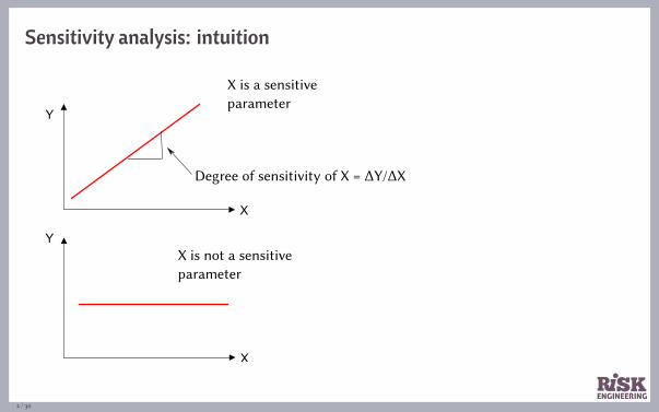
Sensitivity analysis: intuition
X is a sensitiveparameter
Degree of sensitivity of X = ΔY/ΔX
X is not a sensitiveparameter
2 / 30
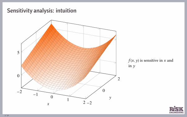
Sensitivity analysis: intuition
−2 −1 0 1 2 −2
0
20
5
𝑥𝑦
f (x , y) is sensitive in x andin y
3 / 30

Sensitivity analysis: intuition
−2 −1 0 1 2 −2
0
20
2
4
𝑥𝑦
f (x , y) is sensitive in x butnot in y
4 / 30
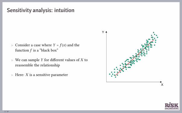
Sensitivity analysis: intuition
▷ Consider a case where Y = f (x ) and thefunction f is a “black box”
▷ We can sample Y for different values of X toreassemble the relationship
▷ Here: X is a sensitive parameter
5 / 30

Sensitivity analysis: intuition
▷ Here, X is not sensitive
▷ Can be “seen” visually
X
Y
6 / 30

Sensitivity analysis: intuition
▷ What can we say about the sensitivity of X?
▷ No graphical interpretation
▷ Consider also functions (or computer models,or spreadsheets) which have tens of inputs• you can’t draw graphs in dimension 23!
▷ We need a more sophisticated method thanscatterplots…
7 / 30

What is sensitivity analysis?
▷ The study of how the variation (uncertainty) in the output of amathematical model can be apportioned, qualitatively or quantitatively, todifferent sources of variation in the model inputs
▷ Answers the question “What makes a difference in this decision problem?”
▷ Can be used to determine whether further research is needed to reduceinput uncertainty before making a decision• information is not free
8 / 30

Sensitivity and uncertainty analysis
simulationmodel
f
Start with a simulation model thatyou want better to understand (oftena computer model). It may be a “blackbox” (you don’t know how it worksinternally).
parameter 1
parameter 2
parameter 3
outputs
uncertainty analysis
Uncertainty analysis: how doesvariability in the inputs propagatethrough the model to variability in theoutputs?
sensitivity analysis
feedback on modelinputs & model structure
Insights gained from the sensitivityanalysis may help to
▷ prioritize effort on reducing inputuncertainties
▷ improve the simulation model
Adapted from figure by A. Saltelli
9 / 30

Sensitivity and uncertainty analysis
simulationmodel
f
Start with a simulation model thatyou want better to understand (oftena computer model). It may be a “blackbox” (you don’t know how it worksinternally).
parameter 1
parameter 2
parameter 3
Define which uncertain input parametersyou want to analyze.
Characterize their probabilitydistributions.
outputs
uncertainty analysis
Uncertainty analysis: how doesvariability in the inputs propagatethrough the model to variability in theoutputs?
sensitivity analysis
feedback on modelinputs & model structure
Insights gained from the sensitivityanalysis may help to
▷ prioritize effort on reducing inputuncertainties
▷ improve the simulation model
Adapted from figure by A. Saltelli
9 / 30
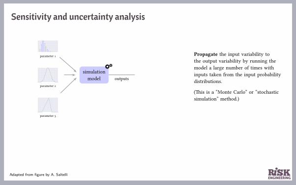
Sensitivity and uncertainty analysis
simulationmodel
f
parameter 1
parameter 2
parameter 3
outputs
Propagate the input variability tothe output variability by running themodel a large number of times withinputs taken from the input probabilitydistributions.
(This is a “Monte Carlo” or “stochasticsimulation” method.)
uncertainty analysis
Uncertainty analysis: how doesvariability in the inputs propagatethrough the model to variability in theoutputs?
sensitivity analysis
feedback on modelinputs & model structure
Insights gained from the sensitivityanalysis may help to
▷ prioritize effort on reducing inputuncertainties
▷ improve the simulation model
Adapted from figure by A. Saltelli
9 / 30

Sensitivity and uncertainty analysis
simulationmodel
f
parameter 1
parameter 2
parameter 3
outputs
uncertainty analysis
Uncertainty analysis: how doesvariability in the inputs propagatethrough the model to variability in theoutputs?
sensitivity analysis Sensitivity analysis: what is therelative contribution of the variabilityin each of the inputs to the total outputvariability?
feedback on modelinputs & model structure
Insights gained from the sensitivityanalysis may help to
▷ prioritize effort on reducing inputuncertainties
▷ improve the simulation model
Adapted from figure by A. Saltelli
9 / 30

Sensitivity and uncertainty analysis
simulationmodel
f
parameter 1
parameter 2
parameter 3
outputs
uncertainty analysis
Uncertainty analysis: how doesvariability in the inputs propagatethrough the model to variability in theoutputs?
sensitivity analysis
feedback on modelinputs & model structure
Insights gained from the sensitivityanalysis may help to
▷ prioritize effort on reducing inputuncertainties
▷ improve the simulation model
Adapted from figure by A. Saltelli
9 / 30
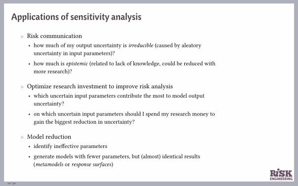
Applications of sensitivity analysis
▷ Risk communication• how much of my output uncertainty is irreducible (caused by aleatory
uncertainty in input parameters)?
• how much is epistemic (related to lack of knowledge, could be reduced withmore research)?
▷ Optimize research investment to improve risk analysis• which uncertain input parameters contribute the most to model output
uncertainty?
• on which uncertain input parameters should I spend my research money togain the biggest reduction in uncertainty?
▷ Model reduction• identify ineffective parameters
• generate models with fewer parameters, but (almost) identical results(metamodels or response surfaces)
10 / 30

Application areas
The European Commission recommends sensitivityanalysis in the context of its impact assessmentguidelines (2009):
‘‘When the assumptions underlying the baseline scenariomight vary as a result of external factors, you need to doa sensitivity analysis to assess whether the impacts of thepolicy options differ significantly for different values ofthe key variables.
Source: EC guidance document at ec.europa.eu/smart-regulation/impact/
11 / 30
Application areas
Principles for Risk Analysis published by the US Office ofManagement and Budget:
‘‘Influential risk assessments should characterize uncertainty with asensitivity analysis and, where feasible, through use of a numericdistribution.
[…] Sensitivity analysis is particularly useful in pinpointing whichassumptions are appropriate candidates for additional datacollection to narrow the degree of uncertainty in the results.Sensitivity analysis is generally considered a minimum, necessarycomponent of a quality risk assessment report.
Source: Updated principles for risk analysis, US OMB, whitehouse.gov/sites/default/files/omb/assets/regulatory_matters_pdf/m07-24.pdf
12 / 30

Sensitivity analysis: the process
1 Specify the objective of your analysis• Example: “Which variables have the most impact on the level of risk?”
2 Build a model which is suitable for automated numerical analysis• Example: spreadsheet with inputs in certain cells and the output of interest in
another cell
• Example: computer code that can be run in batch mode
3 Select a sensitivity analysis method• most appropriate method will depend on your objectives, the time available for
the analysis, the execution cost of the model
4 Run the analysis
5 Present results to decision-makers
13 / 30
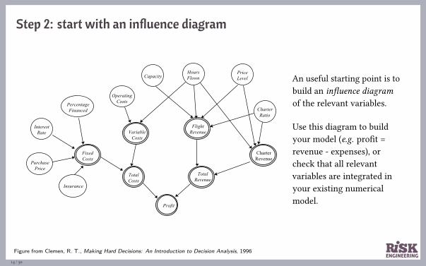
Step 2: start with an influence diagram
An useful starting point is tobuild an influence diagramof the relevant variables.
Use this diagram to buildyour model (e.g. profit =revenue - expenses), orcheck that all relevantvariables are integrated inyour existing numericalmodel.
Figure from Clemen, R. T., Making Hard Decisions: An Introduction to Decision Analysis, 1996
14 / 30

Step 3: sensitivity analysis methods
1 Basic approach: tornado diagram
2 Screening methods
3 oat “one at a time” methods
4 Local sensitivity analysis
5 Global sensitivity analysis
increasingsophistication
more informationavailable
15 / 30

Basic SA: tornado diagram
▷ Tornado diagram: way of presenting basic sensitivity information
• mostly used for project risk management or net present value estimates
• sometimes called “what-if” analysis
▷ Determine lower bound, upper bound and best estimate of each uncertain inputparameter
• = 10%, 90% and 50% quantiles of parameter’s probability distribution
▷ For each uncertain parameter, calculate model output for lower and upper bounds,while taking best estimate for all other uncertain parameters
▷ Draw a horizontal bar for each uncertain parameter between value for lowerbound and value for upper bound
▷ Vertical order of uncertain parameters given by width of the bar
• parameters which lead to large output “spread” (have more impact) at top
▷ Draw a vertical line at position of expected value (model using best estimate forall uncertain parameters)
Market Size
Our Share
Selling Price
Fixed Costs
Variable Cost
0 100 200 300 400 500 600
16 / 30

Tornado diagram example: profit calculation
Profit = (SellingPrice - VariableCost) × MarketSize × MarketShare - FixedCosts
Parameter Lower Expected Upper
Selling price 140 175 200
Market size 8 12 20
Our share 0.18 0.25 0.35
Variable cost 30 40 60
Fixed costs 150 180 300
Market Size
Our Share
Selling Price
Fixed Costs
Variable Cost
0 100 200 300 400 500 600
Interpretation: given these assumptions, the market size parameter hasmost influence on profitability.
Plot generated with free Excel plugin by home.uchicago.edu/ rmyerson/addins.htm
17 / 30

Relevant commercial tools
Example tools with Excel integration:
▷ Palisade TopRank®
▷ Oracle Crystal Ball®
Typically quite expensive…
18 / 30

Screening methods
▷ “Screening” is a preliminary phase that is useful when the model has alarge number of parameters• allows the identification, with a limited number of calculations, of those
parameters that generate significant variability in the model’s output
▷ Simple “oat” (one at a time) screening method: change one factor at atime and look at effect on output• while keeping other factors at their nominal value
, Intuitive approach, can be undertaken by hand
, If model fails, you know which factor is responsible for the failure
/ Approach does not fully explore input space, since simultaneousvariations of input variables are not studied
/ Cannot detect the presence of interactions between input variables
19 / 30

OAT screening method: example
Rosenbrock function: f (x1, x2) = 100(x2 − x21 )
2 + (1 − x1)2
over [-2, 2]²
−2 −1.5 −1 −0.5 0 0.5 1 1.5 2−2
−1
0
1
2
1
101
100
x1
x 2
Both x1 and x2 seem to be sensitive variables in thisexample
> def rosenbrock(x1, x2):return 100*(x2-x1**2)**2 + (1-x1)**2
> rosenbrock(0, 0)1> rosenbrock(1, 0)100> rosenbrock(0, 1)101> rosenbrock(1, 1)0> rosenbrock(-1, -1)404
R e a l m o d el l i n g s i t u a
t i o n s
h a v e m a n ym o r e t h a n
t w o
v a r i a b l e s ,s o o u t p u t
c a n n o t
b e p l o t t e d
20 / 30

The Elementary Effects screening method
▷ The elementary effect for the i-th input variable at x ∈ [0, 1]k is the firstdifference approximation to the derivative of f (·) at x:
EEi(x) =f (x + ∆ei) − f (x)
∆
where ei is the unit vector in the direction of the i-th axis
▷ Intuition: it’s the slope of the secant line parallel to the input axis
▷ Average EEi(x) for various points x in the input domain to obtain ameasure of the relative influence of each factor
𝜇i =1r
r
∑j=1
||EEi(xj )||
21 / 30

Elementary effects method: example
▷ Consider y(x) = 1.0 + 1.5x2 + 1.5x3 + 0.6x4 + 1.7x24 + 0.7x5 + 0.8x6 + 0.5(x5x6)
where• x = (x1, x2, x3, x4, x5, x6)
• 0 ≤ x1, x2, x4, x5, x6 ≤ 1
• 0 ≤ x3 ≤ 5
▷ Note:• y(·) is functionally independent of x1
• y(·) is linear in x2 and x3 and non-linear in x4
• y(·) contains an interaction in x5 and x6
▷ Sensitivity results:• 𝜇1 = 0 as expected
• influence of x4 is highest
• influence of x2 and x3 is equal, as expected
D o w n l o a df u l l d e t a i l s
a s a
P y t h o n n ot e b o o k a t
risk-
engineering.org
0.0 0.5 1.0 1.5 2.0 2.5 3.0Relative sensitivity
μ_1
μ_2
μ_3
μ_4
μ_5
μ_6
Elementary effects
22 / 30

Local sensitivity analysis methods
▷ Local sensitivity analysis: investigation of response stability over a smallregion of inputs
▷ Local sensitivity with respect to a factor is just the partial derivative wrtthat factor, evaluated at that location
▷ Simple example: Rosenbrock function• f (x1, x2) = 100(x2 − x2
1 )2 + (1 − x1)
2, x1, x2 ∈ [−2, 2]
• 𝜕f
𝜕x1= −400x1(−x2
1 + x2) + 2x1 − 2
• 𝜕f
𝜕x2= −200x2
1 + 200x2
23 / 30
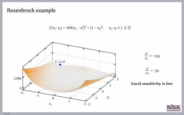
Rosenbrock example
f (x1, x2) = 100(x2 − x21 )
2 + (1 − x1)2, x1, x2 ∈ [−2, 2]
−2−1
01
2 −2
−1
0
1
2
0
2,000
(-1.5,2)
x1
x2
𝜕f
𝜕x1= -155
𝜕f
𝜕x2= -50
Local sensitivity is low
24 / 30

Rosenbrock example
f (x1, x2) = 100(x2 − x21 )
2 + (1 − x1)2, x1, x2 ∈ [−2, 2]
−2−1
01
2 −2
−1
0
1
2
0
2,000
(-2,-2)
x1
x2
𝜕f
𝜕x1= -4806
𝜕f
𝜕x2= -1200
Local sensitivity is high
24 / 30

Rosenbrock example
f (x1, x2) = 100(x2 − x21 )
2 + (1 − x1)2, x1, x2 ∈ [−2, 2]
−2−1
01
2 −2
−1
0
1
2
0
2,000(1,1)
x1
x2
𝜕f
𝜕x1= 0
𝜕f
𝜕x2= 0
Local sensitivity is zero
24 / 30

Local sensitivity analysis methods
▷ The calculation of partial derivatives can be automated for softwarepackages using automatic differentiation methods• the source code must be available
• autodiff.org
▷ This method does not allow you to detect interaction effects betweenthe input variables
▷ Method cannot handle correlated inputs
▷ Widely used for optimization of scientific software
25 / 30

Global sensitivity analysis methods
▷ Examine effect of changes to all input variables simultaneously• over the entire input space you are interested in (for example the uncertainty
distribution of each variable)
▷ Methods based on analysis of variance (often using Monte Carlo methods)
▷ Typical methods that are implemented in software packages:• Fourier Analysis Sensitivity Test (fast), based on a multi-dimensional Fourier
transform
• the method of Sobol’
▷ In general, this is the most relevant method for risk analysis purposes• allows the analysis of interactions between input variables
26 / 30

Sensitivity indices
▷ The sensitivity index of a parameter quantifies its impact on outputuncertainty• measures the part of output variance which can be attributed to variability in
the parameter
▷ Properties:• Si ∈ [0,1]
• ∑i Si = 1
▷ First-order index: Sj =Var(𝔼[z|xj])
Var(z)• measures “main effect”
▷ Total effect index: Tj =𝔼[Var(z|xj)]
Var(z)• measures residual variability due to interactions between xi and other
parameters
27 / 30
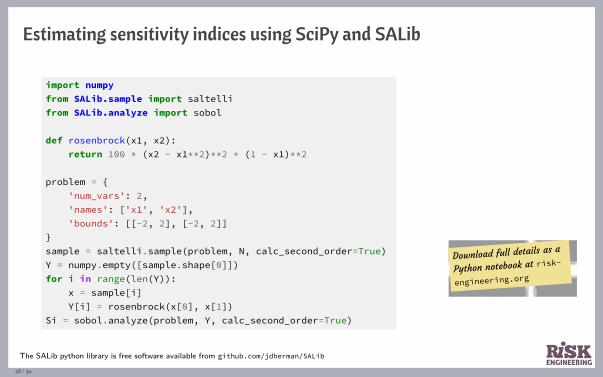
Estimating sensitivity indices using SciPy and SALib
import numpyfrom SALib.sample import saltellifrom SALib.analyze import sobol
def rosenbrock(x1, x2):return 100 * (x2 - x1**2)**2 + (1 - x1)**2
problem = {'num_vars': 2,'names': ['x1', 'x2'],'bounds': [[-2, 2], [-2, 2]]
}sample = saltelli.sample(problem, N, calc_second_order=True)Y = numpy.empty([sample.shape[0]])for i in range(len(Y)):
x = sample[i]Y[i] = rosenbrock(x[0], x[1])
Si = sobol.analyze(problem, Y, calc_second_order=True)
D o w n l o a df u l l d e t a i l s
a s a
P y t h o n n ot e b o o k a t
risk-
engineering.org
The SALib python library is free software available from github.com/jdherman/SALib
28 / 30

Further reading
▷ Appendix on sensitivity analysis of the epa guidance on risk assessment,epa.gov/oswer/riskassessment/rags3adt/pdf/appendixa.pdf
▷ OpenTURNS software platform for uncertainty analysis (free software),openturns.org
▷ Dakota software platform for uncertainty analysis (free software),dakota.sandia.gov
▷ Case study: Using @RISK for a Drug Development Decision: a ClassroomExample, from palisade.com/cases/ISU_Pharma.asp
For more free course materials on risk engineering,visit risk-engineering.org
29 / 30

Feedback welcome!
Was some of the content unclear? Which parts of the lecturewere most useful to you? Your comments [email protected] (email) or@LearnRiskEng (Twitter) will help us to improve these coursematerials. Thanks!
@LearnRiskEng
fb.me/RiskEngineering
google.com/+RiskengineeringOrgCourseware
This presentation is distributed under the terms of theCreative Commons Attribution – Share Alike licence
For more free course materials on risk engineering,visit risk-engineering.org
30 / 30