P O S I V A O Y

FI -27160 OLKILUOTO, F INLAND

Tel +358-2-8372 31

Fax +358-2-8372 3709

Per -Anders Eks t röm

Rober t Broed

May 2006

Work ing Repor t 2006 -31

Sensitivity Analysis Methods and a BiosphereTest Case Implemented in EIKOS

May 2006

Base maps: ©National Land Survey, permission 41/MYY/06

Working Reports contain information on work in progress

or pending completion.

The conclusions and viewpoints presented in the report

are those of author(s) and do not necessarily

coincide with those of Posiva.

Per -Anders Ekst röm

Robert Broed

Fac i l i a AB

Work ing Report 2006 -31

Sensitivity Analysis Methods and a BiosphereTest Case Implemented in EIKOS

ABSTRACT Computer-based models can be used to approximate real life processes. These models are usually based on mathematical equations, which are dependent on several variables. The predictive capability of models is therefore limited by the uncertainty in the value of these. Sensitivity analysis is used to apportion the relative importance each uncertain input pa-rameter has on the output variation. Sensitivity analysis is therefore an essential tool in simulation modelling and for performing risk assessments. Simple sensitivity analysis techniques based on fitting the output to a linear equation are often used, for example correlation or linear regression coefficients. These methods work well for linear models, but for non-linear models their sensitivity estimations are not accurate. Usually models of complex natural systems are non-linear. Within the scope of this work, various sensitivity analysis methods, which can cope with linear, non-linear, as well as non-monotone problems, have been implemented, in a software package, EIKOS, written in Matlab language. The following sensitivity analy-sis methods are supported by EIKOS: Pearson product moment correlation coefficient (CC), Spearman Rank Correlation Coefficient (RCC), Partial (Rank) Correlation Coef-ficients (PCC), Standardized (Rank) Regression Coefficients (SRC), Sobol' method, Jansen's alternative, Extended Fourier Amplitude Sensitivity Test (EFAST) as well as the classical FAST method and the Smirnov and the Cramér-von Mises tests. A graphi-cal user interface has also been developed, from which the user easily can load or call the model and perform a sensitivity analysis as well as uncertainty analysis. The implemented sensitivity analysis methods has been benchmarked with well-known test functions and compared with other sensitivity analysis software, with successful results. An illustration of the applicability of EIKOS is added to the report. The test case used is a landscape model consisting of several linked biosphere compartment models. The model was created in the tool Pandora [PG+05]. The test case serves as an example of how to apply the different sensitivity analysis methods to a model using EIKOS, and also presents results from actual performed model simulations. Keywords: models, uncertainty, sensitivity analysis, non-linear, non-monotone, EIKOS, software

HERKKYYSANALYYSIMENETELMÄT JA BIOSFÄÄRIMALLI TESTAUS-KÄYTTÖÖN TOTEUTETTUNA EIKOS-TYÖKALULLA TIIVISTELMÄ Tietokonepohjaisia malleja käytetään arvioimaan todellisen maailman prosesseja. Nämä mallit pohjautuvat useimmiten useasta muuttujasta riippuviin matemaattisiin yhtälöihin, joten niiden ennustamiskykyä rajoittavat näiden muuttujien arvojen epävarmuudet. Herkkyystarkasteluja käytetään kunkin epävarman syöttöparametrin suhteellisen mer-kityksen selvittämiseen, mikä tekee niistä välttämättömän työkalun simulaatiomallin-nuksessa ja laadittaessa riskiarvioita. Usein käytetään yksinkertaisia herkkyystarkastelumenetelmiä, jotka perustuvat lineaari-sen yhtälön sovitukseen, esimerkiksi korrelaatio- tai lineaarisia regressiokertoimia. Nä-mä menetelmät toimivat tietenkin hyvin lineaarisille malleille, mutta epälineaarisissa tapauksissa ne antavat epätarkkoja tuloksia. Toisaalta monesti monimutkaisten luonnol-listen ilmiöiden mallit ovat juuri epälineaarisia. Tämän työn puitteissa toteutettiin Matlab-kielellä useita eri herkkyystarkastelumenetel-miä, jotka pystyvät käsittelemään lineaarisia, epälineaarisia ja ei-monotonisia malleja. Menetelmistä muodostettiin yhtenäisen graafisen käyttöliittymän sekä mallien lataus- ja kutsutoimintojen avulla ohjelmistopaketti, joka sai nimen EIKOS. Siinä on toteutettuna seuraavat menetelmät: Pearsonin tulomomenttikorrelaatiokerroin (CC), Spearmanin jär-jestyskorrelaatiokerroin (RCC), osittaiset (järjestys)korrelaatiokertoimet (PCC), nor-mitetut (järjestys)regressiokertoimet (SRC), Sobolin menetelmä, Jansenin vaihtoehto, laajennettu Fourier-amplituditesti (EFAST) sekä klassinen FAST menetelmä ja Smirno-vin ja Cramér-von-Misesin testit. Näitä käyttämällä EIKOS-työkalulla voidaan suorittaa kattavasti niin herkkyys- kuin epävarmuusanalyysitkin. Toteutettujen menetelmien toi-minta on varmistettu onnistuneesti vertailemalla hyvin tunnettuihin testifunktioihin ja toisiin herkkyysanalyysiohjelmistoihin. Raportin toinen osa esittelee EIKOS-työkalun käyttöä erään Olkiluodon biosfäärilasku-harjoitusmallin avulla. Tämä malli käsittää useita toisiinsa kytkettyjä kulkeutumismal-leja, ja siten myös runsaasti parametreja, ja se on toteutettu käyttämällä Pandora-työka-lua [PG+05]. Raportissa esitetään miten EIKOS:lla voidaan analysoida eri menetelmiä käyttäen valmiiksi kehitettyä mallia sekä lisäksi tässä testitapauksessa saadut mallin-nustulokset. Avainsanat: mallinnus, epävarmuus, herkkyysanalyysi, epälineaarisuus, ei-monotoni-suus, EIKOS, ohjelmisto

1

TABLE OF CONTENTS ABSTRACT TIIVISTELMÄ TABLE OF CONTENTS........................................................................................... 1 LIST OF ABBREVIATIONS ..................................................................................... 3 1 INTRODUCTION ......................................................................................... 5 2 ANALYSING SENSITIVITY AND UNCERTAINTY ...................................... 7 2.1 Uncertainty analysis......................................................................... 7 2.2 Sensitivity analysis........................................................................... 8 3 SCREENING METHODS............................................................................. 11 3.1 Morris method .................................................................................. 12 3.2 Remarks on screening methods ...................................................... 14 4 SAMPLING-BASED METHODS .................................................................. 17 4.1 Graphical methods........................................................................... 17 4.2 Regression analysis......................................................................... 18 4.3 Correlation coefficients .................................................................... 20 4.4 Rank transformations....................................................................... 21 4.5 Two-sample tests............................................................................. 21 4.6 Remarks on sampling-based methods ............................................ 23 5 VARIANCE-BASED METHODS .................................................................. 25 5.1 Sobol' indices ................................................................................... 27 5.2 Jansen (Winding Stairs)................................................................... 29 5.3 Fourier amplitude sensitivity test...................................................... 31 5.4 Extended Fourier amplitude sensitivity test ..................................... 33 5.5 Remarks on variance-based methods ............................................. 34 6 SUMMARY OF SENSITIVITY ANALYSIS METHODS ................................ 35 7 EXAMPLE OF APPLICATION OF EIKOS ................................................... 37 7.1 The landscape model used in the study .......................................... 37 7.2 Input parameters.............................................................................. 39 7.3 The studied output variables............................................................ 40 7.4 Results of the sensitivity and uncertainty analysis........................... 42 7.4.1 Results of screening study ................................................... 42 7.4.2 Results of the sampling based methods .............................. 46 7.4.3 Results of the Variance based methods .............................. 51 7.4.4 Conclusion of sensitivity analysis......................................... 56 8 CONCLUDING REMARKS .......................................................................... 59 REFERENCES ............................................................................................. 61

APPENDIX 1: COAST MODEL APPLIED ............................................................... 65

APPENDIX 2: LAKE MODEL APPLIED................................................................... 67

APPENDIX 3: RIVER MODEL APPLIED................................................................. 69

2

APPENDIX 4: FOREST MODEL APPLIED ............................................................. 73

APPENDIX 5: REPRODUCING THE RESULTS OBTAINED IN SECTION 7. ........ 75

3

LIST OF ABBREVIATIONS UA Uncertainty Analysis SA Sensitivity Analysis MC Monte Carlo CC Pearson Product Moment Correlation Coefficient RCC Spearman Rank Correlation Coefficient SRC Standardized Regression Coefficient SRRC Standardized Rank Regression Coefficient PCC Partial Correlation Coefficient PRCC Partial Rank Correlation Coefficient FAST Fourier Amplitude Sensitivity Test EFAST Extended Fourier Amplitude Sensitivity Test PDF Probability Distribution Function LHS Latin Hypercube Sampling OAT One-at-a-time WS Winding Stairs eei Elementary effects (for parameter Xi) R2 Model coefficient of determination Si First order sensitivity index (for parameter Xi) STi Total order sensitivity index (for parameter Xi)

4

5

1 INTRODUCTION In the safety assessments and safety case for spent nuclear fuel repositories simulation modelling and environmental risk assessment is applied. Because of the complexity of such models, not to mention the nature itself, analyses of significance of different con-tributors to the uncertainties in predictions with the models are needed. The modern simulation models are usually too complex to allow this kind of assessment been done directly. Thus, software tools capable of the task are needed. EIKOS software is available from Facilia AB. Its development of EIKOS has been sponsored by the Norwegian Radiation Protection Authority (NRPA) and Posiva. The Pandora software [PG+05] used to construct the landscape model for this report has been developed for Posiva and SKB (Svensk Kärnbränslehantering AB) jointly. For testing the compliance of EIKOS with Pandora, testing the workflow and also to gain experience on landscape modelling, i.e. connected ecosystem-specific biosphere model blocks on the basis of terrain and ecosystem development forecasts, a modelling exercise was also conducted to be reported as a test case for EIKOS/Pandora system. This report has been organised into two main parts. The first part begins with a brief introduction to sensitivity analysis, followed by a theoretical text about main sensitivity analysis techniques incorporated in EIKOS, these methods are divided into

• Screening methods • Sampling-based methods • Variance-based methods

In the second part a biosphere test case implemented in Pandora and analysed using EIKOS is presented and thoroughly discussed.

6

7

2 ANALYSING SENSITIVITY AND UNCERTAINTY A simulation modelling and risk assessment tool, such as Pandora [PG+05], should in-clude procedures for sensitivity analysis, which can be used to assess the influence of different model parameters on simulation endpoints. Such assessments are needed for ranking the parameters in order of importance serving various purposes, for example:

• to identify major contributors to the uncertainties in the predictions with a model,

• to identify research priorities to improve risk assessments with a model. In the following text, the model is seen as a black box function f with k input parameters x=(x1, x2,…, xk) and one single scalar output y, i.e.

),...,,f( 21 kxxxy = . (1)

In an application y may have a higher dimensionality, for example it could be a vector instead of a scalar. The term input parameter is used to denote any quantity that can be changed in the model prior to its execution. It may be, for example, a parameter, an ini-tial value, a variable or a module of the model.

2.1 Uncertainty analysis The input parameters of models are not always known with a sufficient degree of cer-tainty. Input uncertainty can be caused by natural variability as well as by errors and uncertainties associated with measurements. In this context, the model is assumed to be deterministic, i.e. the same input data would produce the same output if the model was run twice. Therefore, the input uncertainties are the only uncertainty propagated through the model affecting the output uncertainty. The uncertainty of input parameters is often expressed in terms of probability distribu-tions; which can also be derived from samples of measured values, i.e. empirical prob-ability distributions. The different input parameters may have dependencies on each other, i.e. they may be correlated. Generally, the main reason of performing an uncertainty analysis is to assess the uncer-tainty in the model output that derives from uncertainty in the inputs. The question to be investigated is: How does y vary when x varies according to some assumed joint prob-ability distributions?

8

2.2 Sensitivity analysis Andrea Saltelli [Sal00] states that Sensitivity analysis (SA) is the study of how the varia-tion in the output of a model (numerical or otherwise) can be apportioned, qualitatively or quantitatively, to different sources of variation, and how the given model depends upon the information fed into it. Saltelli also lists a set of reasons why modellers should carry out a sensitivity analysis, these are to determine:

a) if a model resembles the system or processes under study; b) the parameters that mostly contribute to the output variability; c) the model parameters (or parts of the model itself) that are insignificant; d) if there is some region in the space of input parameters for which the model

variation is maximal; e) the optimal regions within the space of the parameters for use in a subsequent

calibration study; f) if and which (group of) parameters interact with each other.

Local and global sensitivity analysis Sensitivity analysis aims at determining how sensitive the model output is to changes in model inputs. When input parameters are relatively certain, we can look at the partial derivative of the output function with respect to the input parameters. This sensitivity measure can easily be computed numerically by performing multiple simulations vary-ing input-parameters around a nominal value. We will find out the local impact of the parameters on the model output and therefore techniques like these are called local sen-sitivity analysis. For environmental and health risk assessments, input parameters will often be uncertain and therefore local sensitivity analysis techniques will not be usable for a quantitative analysis. We want to find out which of the uncertain input parameters are more important in determining the uncertainty in the output of interest. To find this we need to consider global sensitivity analysis, which are usually implemented using Monte Carlo (MC) simulation and are, therefore, called sampling-based methods.

Choice of an appropriate method Different sensitivity analysis techniques will do well on different types of model prob-lems. At an initial phase, for models with a large amount of uncertain input parameters, a screening method could be used to qualitatively find out which the most important pa-rameters are and which are not important. The screening method implemented in EIKOS is the Morris design [Mor91]. A natural starting point in the analysis with sam-pling-based methods would be to examine scatter plots. With these, the modeller can graphically find out nonlinearities, nonmonotonicity and correlations between the input-output parameters.

9

For linear models, linear relationship measures like Pearson product moment correlation coefficient (CC), Partial Correlation Coefficients (PCC) and Standardized Regression Coefficients (SRC) will be adequate. For non-linear but monotonic models, measures based on rank transforms like Spear-man Rank Correlation Coefficient (RCC), Partial Rank Regression Coefficient (PRCC) and Standardized Rank Regression Coefficients (SRRC) will perform well. For non-linear non-monotonic models, methods based on decomposing the variance are the best choice. Examples of these methods are the Sobol' method, Jansen's alternative, the Fourier Amplitude Sensitivity Test (FAST) and the Extended Fourier Amplitude Sensitivity Test (EFAST). Methods of partitioning the empirical input distributions according to quantiles1 (or other restrictions) of the output distribution are called Monte Carlo filtering. Measures of their difference are called two-sample-tests. Two non-parametric2 two-sample-tests are implemented: the Smirnov and the Cramér-von Mises tests.

1 The q-quantile of a random variable X is any value x such that the probability P(X≤x)=q. 2 Non-parametric -- minimal or no assumptions are made about the probability distributions of the pa-rameters being assessed.

10

11

3 SCREENING METHODS When dealing with computationally laborious models, containing large amounts of un-certain input parameters, screening methods can be used to isolate the set of parameters that has the strongest effect on the output variability by performing only a few model runs. This way the number of uncertain input parameters to examine might be reduced. It is often the case that the number of significant input parameters is quite small com-pared to the total number of input parameters in a model. The most appealing property of the screening methods is their low computational costs i.e. the required number of model runs. A drawback of this feature is that the sensitivity measure is only qualitative in the sense that the input parameters are ranked in order of significance, but their absolute contribution is not quantified. There are various screening techniques described in the literature. One of the simplest is the one-parameter-at-a-time design (OAT). In this design the input parameters are var-ied in turn and the effect each has on the output is measured. Normally, the parameters that are not varied are fixed at nominal values. A maximum and minimum value is often used representing the range of likely values for each parameter. Usually the nominal value is chosen to be mean of these extremes. The OAT design can be used to compute the local impact of the input parameters on the model outputs thus this method is often referred to as local sensitivity analysis. It is usually carried out by computing partial derivatives of the output functions with respect to the input variables. The approach often seen in the literature is, instead of computing derivatives, to vary the input parameters in a small interval around the nominal value. The interval is usually a fixed (e.g. 5%) fraction of the nominal value and is not related to the uncertainty in the value of the parameters. In general, the number of model runs required for an OAT design is of the order O(k) (often, 2k+1), k being the number of parameters examined. An elementary OAT design for computing the local impact of the input parameters is implemented in EIKOS. In this design one choose a nominal value and extremes for each input parameter, or assign a fraction of variation of the nominal value. EIKOS then varies each parameter in turn to compute local sensitivities (partial derivatives) if the extremes are not too far away from the nominal values and the model relationship is lin-ear this approximation will be accurate.

12

−0.3562 0 0.3562

X1

X2

X3

X1: 5%

X2: 14%

X3: 32%

Unexplained: 49%

Figure 3.1. Example of results from performing a local sensitivity analysis, illustrated as a tornado and a pie chart. The result clearly indicates that parameter X3 has the most impact on the model prediction.

3.1 Morris method Morris [Mor91] came up with an experimental plan that is composed of individually randomised OAT designs. The data analysis is then based on the so-called elementary effects, the changes in an output due to changes in a particular input parameter in the OAT design. The method is global in the sense that it does vary the input values over their whole range of uncertainty. The Morris method can determine if the effect of the input parameter xi on the output y is negligible, linear and additive, nonlinear or in-volved in interactions with other input parameters x~i

3.

−30 −20 −10 0 10 20 30 40 500

10

20

30

40

50

60

70

80

90

←X1

←X2←X3

←X4

←X5

←X6

←X7

←X8

←X9←X10

←X11

←X12

←X13

←X14

←X15←X16

←X17

←X18←X19←X20

Estimated means (µ)

Sta

ndar

d D

evia

tions

(σ)

Figure 3.2. Example of results from performing a sensitivity analysis using Morris method 3 xi is the input parameter under consideration; x~i is all input parameters, except the input parameter un-der consideration.

13

According to Morris if:

a) f(xi+∆, x~i) - f(x) is nonzero, then xi affects the output. b) f(xi+∆, x~i) - f(x) varies as xi varies, then xi affects the output nonlinearly. c) f(xi+∆, x~i) - f(x) varies as x~i varies, then xi affects the output with interactions

with other inputs.

where ∆ is the variation size. The input parameter space is discretised and the possible input parameter values will be restricted to be inside a regular k-dimensional p-level grid, where p is the number of levels of the design. The elementary effect of a given value xi of input parameter Xi is defined as a finite-difference derivative approximation:

∆−∆+= +− /)]f(),...,,,,...,,[f()( 1121 xx kiiii xxxxxxee (2)

for any xi between 0 and 1-∆ where x 1),...,1/(2),1/(1,0 −−∈ ppx , and ∆ is a prede-termined multiple of 1/(p-1). The influence of xi is then evaluated by computing several elementary effects at randomly selected values of xi and x~i. If all samples of the elementary effect of the i'th input parameter are zero, then xi does not have any effect on the output y, the sample mean and standard deviation will both be zero. If all elementary effects have the same value, then y is a linear function of xi. The standard deviation of the elementary effects will then equal zero. For more complex in-teractions, due to interactions between parameters and nonlinearity, Morris state [Mor91] that if the mean of the elementary effects is relatively large and the standard deviation is relatively small, the effect of xi on y is mildly nonlinear. If the opposite, i.e. the mean is relatively small and the standard deviation is relatively large, then the effect is supposed to be strongly nonlinear. As a rule of thumb:

a) a high mean of elementary effects indicates a parameter with an important over-all influence on the output and

b) a high standard deviation in elementary effects indicates that either the parame-ter is interacting with other parameters or the parameter has nonlinear effects on the output.

To compute r elementary effects of the k inputs we need to do 2rk model evaluations. With the use of the Morris randomized OAT design the number of evaluations are re-duced to r(k+1). The design that Morris proposed [Mor91] is based on the construction of a (k+1)×k ori-entation matrix B*. Rows in B* represent input vectors x=x(1), x(2),…, x(k+1) that define a trajectory4 in the input parameter space, for which the corresponding experiment pro- 4 Trajectory -- A sequence of points starting from a random base vector in which two consecutive ele-ments differ only for one component.

14

vides k elementary effects, one for each input parameter. The algorithm of Morris de-sign is:

a) Randomly choose a base value x* for x, sampled from the set 0,1/(p-1),2/(p-1),…,1-∆.

b) One or more of the k elements in x are increased by ∆. c) The estimated elementary effect of the i'th component of x(1) is (if changed by ∆)

eei(x(1))=[f(x1(1),x2

(1),…,xi-1(1),xi

(1)+∆,xi+1(1),…,xk

(1))-f(x(1))]/∆ if x(1) has been increased by ∆, or eei(x(1))=[f(x(1))-f(x1

(1),x2(1),…,xi-1

(1),xi(1)+∆,xi+1

(1),…,xk(1))]/∆

if x(1) has been decreased by ∆ d) Let x(2) be the new vector (x1

(1),x2(1),…,xi-1

(1),xi(1)±∆,xi+1

(1),…,xk(1)) defined above.

Select a new vector x(3) such that x(3) differs from x(2) for only one component j: either xj

(3)=xj(2)+∆ or xj

(3)=xj(2)-∆, j≠i. Estimated elementary effect of parameter j

is then eej(x(2))=(f(x(3))-f(x(2)))/∆, if ∆ > 0, or eej(x(2))=(f(x(2))-f(x(3)))/∆, other-wise.

e) The previous step is then repeated such that a succession of k+1 input vectors x(1),x(2),…,x(k+1) is produced with two consecutive vectors only differing in one component.

To produce the randomised orientation matrix B* containing the k+1 input vectors, Mor-ris proposed:

)))2)((2/(( *1

*1

*1,1

* PJDJBJB ,kk,kkk x +++ +−∆+= , (3)

where Jk+1,k is a (k+1)×k matrix of ones, B is a (k+1)×k sampling matrix which has the property that for every of its column i=1, 2,…, k, there are two rows of B that differ only in their i'th entries. D* is a k-dimensional diagonal matrix with elements ±1 and finally P* is a k×k random permutation matrix, in which each column contains one ele-ment equal to 1 and all the others equal to 0, and no two columns have ones in the same position. B* provides one elementary effect per parameter that is randomly selected, r different orientation matrices B* have then to be selected in order to provide an r×k-dimensional sample.

3.2 Remarks on screening methods The main advantage of the Morris design is the relatively low computational cost. The design requires only about one model run per computed elementary effect. One drawback with the Morris design is that it only gives an overall measure of the in-teractions, indicating whether interactions exists, but it does not reveal which are the most significant. Also it can only be used with a set of orthogonal input parameters, i.e. correlations cannot be induced on the input parameters.

15

In an implementation, there is a need to think about the choice of the p levels among which each input parameter is varied. In EIKOS, these levels correspond to quantiles of the input parameter distributions, if the distributions are not uniform. For uniform dis-tributions, the levels are obtained by dividing the interval into equidistant parts. The choice of the sizes of the levels p and realizations r is also a problem; various ex-perimenters have demonstrated that the choice of p=4 and r=10 produces good results [STCR04].

16

17

4 SAMPLING-BASED METHODS The sampling-based methods are among the most commonly used techniques in sensi-tivity analysis. They are computed on the basis of the mapping between the input-output-relationship generated by Monte Carlo simulation. Sampling-based methods are sometimes called global since these methods evaluate the effect of xi while all other in-put parameters xj, j≠i, are varied simultaneously. All input parameters are varied over their entire range. This in contrast to local perturbation approaches where the effect of xi is evaluated when the others xj, j≠i, are kept constant at a nominal value. In the rest of this section various common sampling-based sensitivity analysis methods are described.

4.1 Graphical methods Providing a means of visualizing the relationships between the output and input parame-ters, graphical methods play an important role in sensitivity analysis. A plot of the points [Xij,Yj] for j=1,2,…,N, usually called a scatter plot Figure 4.1 can reveal nonlinear or other unexpected relationships between the input parameter xi and the output y.

0.01 0.02 0.03 0.04 0.05 0.06 0.07 0.08 0.090.91

0.92

0.93

0.94

0.95

0.96

0.97

0.98

0.99

Y

X

Figure 4.1. Example of a scatter plot with an overlay of a regression line.

18

Scatter plots are undoubtedly the simplest sensitivity analysis technique, and they are a natural starting point in the analysis of a complex model. They facilitate the understand-ing of model behaviour and the planning of more sophisticated sensitivity analysis. When only one or two inputs dominate the outcome, scatter plots alone often com-pletely reveal the relationships between the model input X and output Y. Using Latin hypercube sampling can be particularly revealing due to the full stratifica-tion over the range of each input variable. A tornado graph Figure 4.2 is another type of plot often used to present the results of a sensitivity study. It is a simple bar graph where the sensitivity statistics is visualized vertically in order of descending absolute value. All of the global sensitivity measures presented in this section can be presented with a tornado graph.

−0.084 0 0.084

X4

X6

X7

X1

X5

X3

X2

Figure 4.2. Example of a tornado chart.

4.2 Regression analysis A sensitivity measure of a model can be obtained using a multiple regression to fit the input data to a theoretical equation that could produce the output data with as small er-ror as possible. The most common technique of regression in sensitivity analysis is the least squares linear regression. Thus the objective is to fit the input data to a linear equa-tion ( baXY +=ˆ ) approximating the output Y, with the criterion that the sum of the squared difference between the line and the data points in Y is minimized. A linear re-gression model of the N×k input sample X to the output Y takes the form:

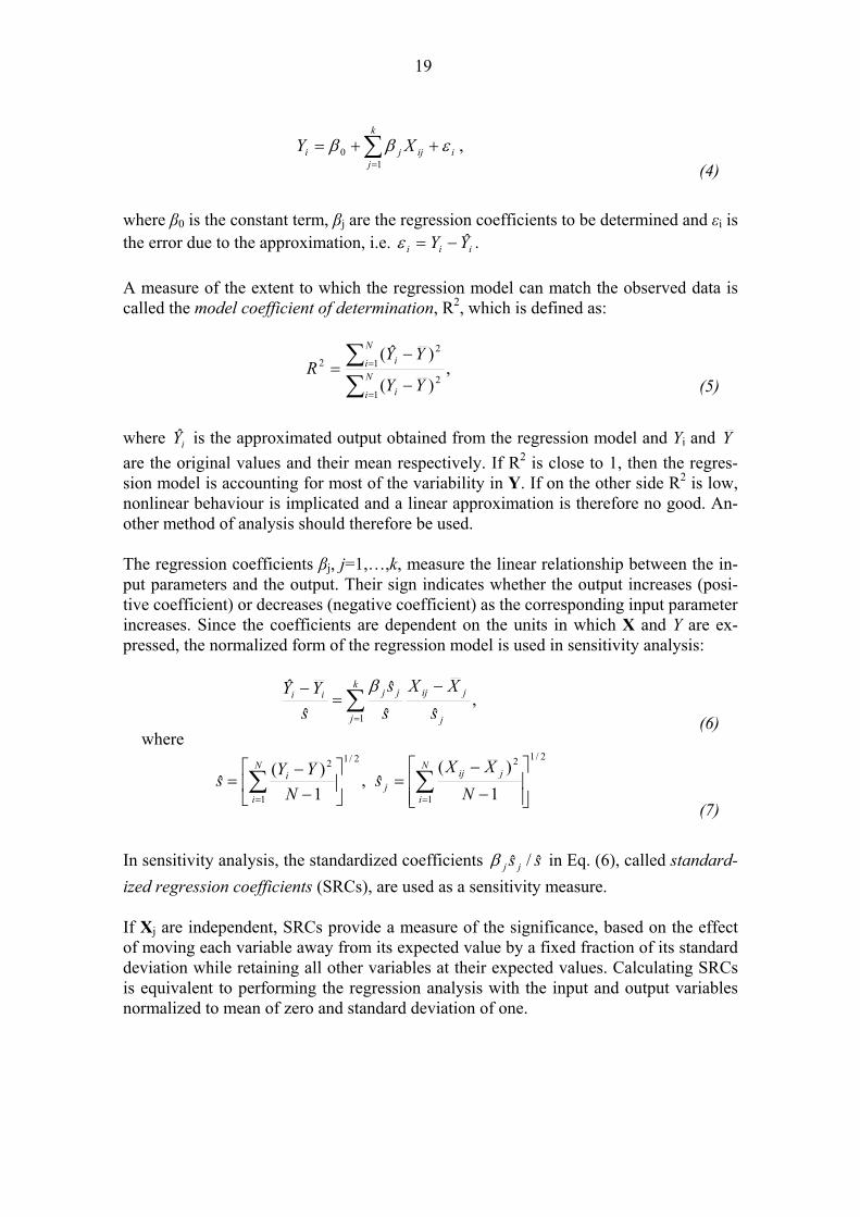
19

∑=

++=k

jiijji XY

10 εββ ,

(4)

where β0 is the constant term, βj are the regression coefficients to be determined and εi is the error due to the approximation, i.e. iii YY ˆ−=ε . A measure of the extent to which the regression model can match the observed data is called the model coefficient of determination, R2, which is defined as:

,)(

)ˆ(

12

12

2

∑∑

=

=

−

−= N

i i

N

i i

YY

YYR

(5)

where iY is the approximated output obtained from the regression model and Yi and Y are the original values and their mean respectively. If R2 is close to 1, then the regres-sion model is accounting for most of the variability in Y. If on the other side R2 is low, nonlinear behaviour is implicated and a linear approximation is therefore no good. An-other method of analysis should therefore be used. The regression coefficients βj, j=1,…,k, measure the linear relationship between the in-put parameters and the output. Their sign indicates whether the output increases (posi-tive coefficient) or decreases (negative coefficient) as the corresponding input parameter increases. Since the coefficients are dependent on the units in which X and Y are ex-pressed, the normalized form of the regression model is used in sensitivity analysis:

,ˆˆ

ˆˆ

ˆ

1 j

jijk

j

jjii

sXX

ss

sYY −

=− ∑

=

β

where

,1)(

ˆ2/1

1

2

⎥⎦

⎤⎢⎣

⎡−

−= ∑

=

N

i

i

NYY

s 2/1

1

2

1)(

ˆ⎥⎥⎦

⎤

⎢⎢⎣

⎡

−

−= ∑

=

N

i

jijj N

XXs

(6)

(7)

In sensitivity analysis, the standardized coefficients ss jj ˆ/ˆβ in Eq. (6), called standard-ized regression coefficients (SRCs), are used as a sensitivity measure. If Xj are independent, SRCs provide a measure of the significance, based on the effect of moving each variable away from its expected value by a fixed fraction of its standard deviation while retaining all other variables at their expected values. Calculating SRCs is equivalent to performing the regression analysis with the input and output variables normalized to mean of zero and standard deviation of one.

20

4.3 Correlation coefficients The correlation coefficients (CC) usually known as Pearson's product moment correla-tion coefficients, provide a measure of the strength of the linear relationship between two variables. The CC between two N-dimensional vectors x and y is defined by

[ ] [ ] ,)()(

))((2/1

122/1

12

1

∑∑∑

==

=

−−

−−=

N

k kN

k k

N

k kkxy

yyxx

yyxxρ

(8)

where x and y are defined as the mean of x and y respectively. The CC could be re-formulated as

,)()(),cov(

yxyx

xy σσρ =

(9)

where cov(x,y) is the covariance between the data sets x and y and σ(x) and σ(y) are the sampled standard deviations. Thus, the correlation coefficient is then the normalized covariance between the two data sets and, as SRC, it produces a unitless index between -1 and +1. The CC is equal in absolute value to the square root of the model coefficient of determination R2 associated with the linear regression. The CC only measures the linear relationship between two variables without consider-ing the effect that other possible variables might have. So when more than one input pa-rameters are under consideration, as it usually is, partial correlation coefficients (PCCs) can be used instead to provide a measure of the linear relationships between two vari-ables when all linear effects of other variables have been removed. The PCC between an individual variable Xi and Y can be obtained from the use of a sequence of regression models. The procedure begins with constructing the following regression models:

∑≠=

+=k

ijjjji XccX

,10

ˆ and ∑≠=

+=k

ijjjji XbbY

,10

ˆ . (10)

Then PCC is defined by the CC of ii XX ˆ− and YY ˆ− . PCC can also be written in terms of simple correlation coefficients by denoting the PCC of X1 and Y while holding Z=X2,…, Xk fixed as ρX1Y|X2,…,Xk, then

)1)(1( 22|11

1

YZZX

YZZXYXZYX

iρρ

ρρρρ

−−

−= .

(11)

21

Partial correlation coefficients characterize the strength of the linear relationship be-tween two variables after a correction has been made for the linear effects of the other variables in the analysis. Standardized regression coefficients on the other hand charac-terize the effect on the output variable that results from perturbing an input variable by a fixed fraction of its standard deviation. Thus, PCC and SRC provide related, but not identical, measures of the significance of the variable. When input parameters are un-correlated, results from PCC and SRC are identical.

4.4 Rank transformations Since the above methods are based on the assumption of linear relationships between the input-output parameters, they will perform poorly if the relationships are nonlinear. Rank transformation of the data can be used to transform a nonlinear but monotonic re-lationship to a linear relationship. When using rank transformation, the data is replaced with their corresponding ranks. Ranks are defined by assigning 1 to the smallest value, 2 to the second smallest and so-on, until the largest value has been assigned the rank N. If there are ties in the data set, then the average rank is assigned to them. The usual regres-sion and correlation procedures are then performed on the ranks instead of the original data values. Standardized rank regression coefficients (SRRC) are SRC calculated on ranks, spearman rank correlation coefficient (RCC) are corresponding CC calculated on ranks and partial rank correlation coefficients (PRCC) are PCC calculated on ranks. The model coefficient of determination R2 in Eq. (5) can be computed with the ranked data and measures then how well the model matches the ranked data. Rank-transformed statistics are more robust, and provide a useful solution in the pres-ence of long tailed input-output distributions. A rank-transformed model is not only more linear, but it is also more additive. Thus the relative weight of the first-order terms is increased on the expense of higher-order terms and interactions.

4.5 Two-sample tests Two-sample tests were originally designed to check the hypothesis of two different samples belonging to the same population [Con99]. In sensitivity analysis, two-sample tests can be used together with Monte Carlo filtering. In Monte Carlo filtering the input samples are partitioned into two sub-samples according to restrictions on the output dis-tribution. The two-sample test is then performed on the two empirical cumulative distri-butions of the sub-samples, and measured if their difference is significant or not, i.e. if the two distributions are different, it can be said that the parameter influences the out-put. The Smirnov test is defined as the greatest vertical distance between the two empirical cumulative distributions:

22

0 0.2 0.4 0.6 0.8 10

0.1

0.2

0.3

0.4

0.5

0.6

0.7

0.8

0.9

1

PriorF

n(x

i|Bhat)

Fm

(xi|B)

Figure 4.3. Example of difference plot of two empirical samples.

|,)(F)(F|max),smirnov( 21 jjXj XXXYj

−= (12)

where F1(x) and F2(x) are the cumulative distributions of Xi estimated on the two sub-samples and the difference is estimated at all the xij points, i=1,…,N. A test similar to the Smirnov test, but with slightly more calculations, is the Cramér-von Mises test, which is given by:

,))(F)((F)(

),cramer( 2212

21

21 ∑ −+

=jX

iij XXNN

NNXY

(13)

where the squared difference in the summation is computed at each xij, i.e. the statistic depends upon the total area between the two distributions.

23

4.6 Remarks on sampling-based methods According to Saltelli et al. [SM90, SH91] the estimators PRCC and SRRC appears to be, in general, the most robust and reliable methods of the ones described in this section, followed by Spearman's RCC and the Smirnov test. Nevertheless, all above tests have been included in EIKOS since they could be of use in different contexts. The rankings of SRCC and PRCC are usually identical, so they could be considered re-dundant. Differences occur only when there are significant correlations amongst the in-put parameters. Predictions using SRRC are strongly correlated to those of Spearman's RCC and the Smirnov test. Therefore, the value of the model coefficient of determination R2 plays a crucial role, as it indicates the degree of reliability of the regressed model in SRRCs as well as the other techniques.

24

25

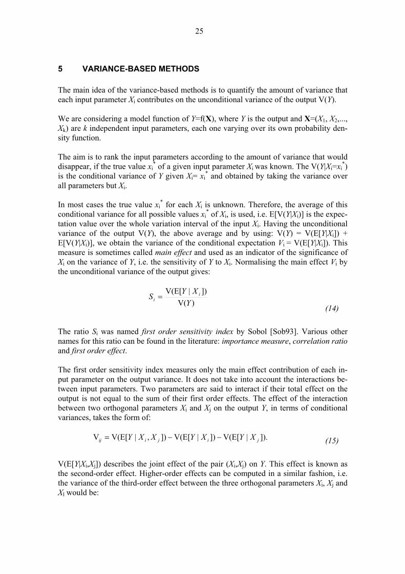
5 VARIANCE-BASED METHODS The main idea of the variance-based methods is to quantify the amount of variance that each input parameter Xi contributes on the unconditional variance of the output V(Y). We are considering a model function of Y=f(X), where Y is the output and X=(X1, X2,..., Xk) are k independent input parameters, each one varying over its own probability den-sity function. The aim is to rank the input parameters according to the amount of variance that would disappear, if the true value xi

* of a given input parameter Xi was known. The V(Y|Xi=xi*)

is the conditional variance of Y given Xi= xi* and obtained by taking the variance over

all parameters but Xi. In most cases the true value xi

* for each Xi is unknown. Therefore, the average of this conditional variance for all possible values xi

* of Xi, is used, i.e. E[V(Y|Xi)] is the expec-tation value over the whole variation interval of the input Xi. Having the unconditional variance of the output V(Y), the above average and by using: V(Y) = V(E[Y|Xi]) + E[V(Y|Xi)], we obtain the variance of the conditional expectation Vi = V(E[Y|Xi]). This measure is sometimes called main effect and used as an indicator of the significance of Xi on the variance of Y, i.e. the sensitivity of Y to Xi. Normalising the main effect Vi by the unconditional variance of the output gives:

)V(])|V(E[

YXY

S ii =

(14)

The ratio Si was named first order sensitivity index by Sobol [Sob93]. Various other names for this ratio can be found in the literature: importance measure, correlation ratio and first order effect. The first order sensitivity index measures only the main effect contribution of each in-put parameter on the output variance. It does not take into account the interactions be-tween input parameters. Two parameters are said to interact if their total effect on the output is not equal to the sum of their first order effects. The effect of the interaction between two orthogonal parameters Xi and Xj on the output Y, in terms of conditional variances, takes the form of:

]).|V(E[])|V(E[]),|V(E[V jijiij XYXYXXY −−= (15)

V(E[Y|Xi,Xj]) describes the joint effect of the pair (Xi,Xj) on Y. This effect is known as the second-order effect. Higher-order effects can be computed in a similar fashion, i.e. the variance of the third-order effect between the three orthogonal parameters Xi, Xj and Xl would be:

26

.VVVVVV]),,|V(E[V ljijlilijljiijl XXXY −−−−−−= (16)

A model without interactions is said to be additive, for example a linear model is always additive. The first order indices sums up to one in an additive model with orthogonal inputs. For additive models, the first order indices coincide with outputs of regression methods (described in section 3.2). For non-additive models information from all inter-actions is seeked for, as well as the first order effect. For non-linear models the sum of all first order indices can be very low. The sum of all the order effects that a parameter accounts for is called the total effect [HS96]. So for an input Xi, the total sensitivity in-dex STi is defined as the sum of all indices relating to Xi (first and higher order). Having a model with three input parameters (k=3), the total sensitivity index for input parameter X1 would then be

123131211SSSSST +++= . (17)

Computing all order-effects to obtain the total effect by brute force is not advisable when the number of input parameters k increases, since the number of terms needed to be evaluated are as many as 2k-1. In the following subsections, four methods to obtain these sensitivity indices are de-scribed. These are the Sobol' indices, Jansen's Winding Stairs technique, Fourier Ampli-tude Sensitivity Test (FAST) and the Extended Fourier Amplitude Sensitivity Test (EFAST). All four methods, except FAST, can obtain both the first and total order ef-fect in an efficient way. The standard FAST method only computes the first order effect. The Sobol method can achieve all order effects, but the need of model runs increases too much to be practical. The input parameter space Ωk is hereafter assumed to be the k-dimensional unit hyper-cube: Ωk = (X | 0 ≤ Xi ≤ 1, i = 1,…, k). This does not give any loss of generality since the parameters can be deterministically transformed from the uniform distributions to a general probability distribution function. The input parameters are also assumed to be orthogonal against each other, thus no correlation structure can be induced on the input parameters. The expected value of the output E(Y) can be evaluated by the k-dimensional integral as

,)f()p()f()E( ∫∫ ΩΩ==

kkddY XXXXX (18)

where p(X) is the joint probability density function assumed to be uniform for each in-put parameter.

27

5.1 Sobol' indices Sobol [Sob93] introduced the first order sensitivity index by decomposing the model function f into summands of increasing dimensionality:

).,...,(f...),(f)(ff),...,f( 1...11 11

01 kk

k

l

k

ijjiij

k

iiik XXXXXXX ∑ ∑∑

= +==

++++= (19)

This representation of the model function f(X), holds if f0 is a constant (f0 is the expec-tation of the output, i.e. E(Y)) and the integrals of every summand over any of its own variables are zero, i.e.:

,0),...,(f1

1

0=∫ ksi iiii dXXX if sk ≤≤1 . (20)

As a consequence of this, all the summands are mutually orthogonal. The total variance V(Y) is defined as

20

2 f)(f)V( −= ∫ΩkdY XX (21)

and the partial variances are computed from each of the terms in Eq. (19)

ssss iiiiiiii dXdXXX ,...,),...,(f...V1111

1

0

2...

1

0... ∫∫= , (22)

where 1 ≤ i1 <…< is ≤ k. The sensitivity indices are then obtained by

,)V(

V ......

1

1 YS s

s

iiii =

(23)

for 1 ≤ i1 <…< is ≤ k. The integrals in Eq. (21) and Eq. (22) can be computed with Monte Carlo methods. For a given sample size N the Monte Carlo estimate of f0 is:

∑=

=N

mmN 1

0 )f(1f X , (24)

where Xm is a sampled point in the input space Ωk.

28

The Monte Carlo estimate of the output variance V(Y) is

20

1

2 f)(f1)(V −= ∑=

N

mmN

Y X , (25)

The main effect of input parameter Xi is estimated as

.f),f()f(1V 20

1

)1()2(~

)1(~ −= ∑

=

N

m

Mim

Mim

Mimi X

NXX

(26)

where two sampling matrices, X(M1) and X(M2), are used; both of size N×k. )1(~MimX identi-

fies the full set of samples from X(M1) except the i'th one. Matrix X(M1) is usually called the data base matrix while X(M2) is called the resampling matrix [CST00]. For formulas of computing partial variances of higher order than in Eq. (26), a separate Monte Carlo integral is required to compute any effect, as further discussed in [HS96]. Counting the Monte Carlo integrals needed for computing 0f , a total of 2k Monte Carlo integrals are therefore needed for a full characterization of the system. In 1996, Homma and Saltelli proposed an extension for direct evaluation of the total sensitivity index STi [HS96]: STi can be evaluated with just one Monte Carlo integral instead of computing the 2k integrals. They suggested dividing the set of input parame-ters into two subsets, one containing the given variable Xi and the other containing its complementary set Xci. The decomposition of f(X) would then become:

),(f)(f)(ff)f( ,0 ciiciiciciii XX XXX +++= . (27)

The total output variance V(Y) would be

ciiciiY ,VVV)V( ++= , (28)

and the total effect sensitivity index STi

ciciiiT SSSSi

−=+= 1, . (29)

Thus, to obtain the total sensitivity index for variable Xi we only need to obtain its com-plementary index Sci=Vci/V(Y). Homma and Saltelli [HS96] shows that Vci can be esti-mated with just one Monte Carlo integral, as

.f),f(),f(1V 20

1

)2()1(~

)1()1(~ −= ∑

=

N

m

Mim

Mim

Mim

Mimci XX

NXX (30)

29

The first and total order sensitivity indices can be computed as: )(V/V YS ii = and )(V/V1 YS ciTi

−= respectively. To obtain both first and total order sensitivity indices for k parameters and N samples, with Sobol' method, we need to make N(2k+1) model runs if either X(M1) or X(M2) is used to compute the unconditional variance V(Y) as described in Eq. (25). When the mean value (f0) is large, a loss of accuracy is induced in the computation of the variances by the Monte Carlo methods presented above [Sob01]. If c0 is defined as an approximation to the mean value f0, the new model function f(x)-c0 can be used in-stead of the original model function (f(x)) in the analysis. For the new model function, the constant term will then be very small, and the loss of accuracy, due to a large mean value, will disappear. This transformation is, however, not implemented in EIKOS. When computing Sobol' indices, the standard Monte Carlo sampling schemes are usu-ally not used, in favour of Sobol's LPτ sequences. LPτ sequences are quasi-random se-quences used to produce points uniformly distributed in the unit hypercube. The differ-ence between quasi-random numbers and uncorrelated pseudo-random numbers is that the quasi-random numbers maintain a nearly uniform density of coverage of the domain while pseudo-random numbers may have places that are relatively undersampled and other places that have clusters of points. The main reason to use quasi-random numbers instead of pseudo-random numbers in a Monte Carlo simulation is that the former con-verge faster [Sob01]. Algorithms to produce LPτ sequences have not yet been incorporated in EIKOS, thus the Sobol' indices has to be computed on the basis of pseudo-random numbers.

5.2 Jansen (Winding Stairs) Chan, Saltelli and Tarantola [CST00] proposed the use of a new sampling scheme to compute both first and total order sensitivity indices in only N×k model runs. The sam-pling method used to measure the main effect was called Winding Stairs, developed by Jansen, Rossing and Deemen in 1994 [JRD94]. The main effect is computed as

,)],f(),E[f(21)V(V 2'

~~ iiiiJ

i XXY XX −−= (31)

and the total effect is computed as

.)],f(),E[f(21V 2

~'

~ iiiiJ

T XXi

XX −= (32)

Here (Xi,X´~i) denotes that all variables are resampled, except for the i'th one. Jansen's method uses the squared differences of two sets of model outputs to compute the indices

30

whereas the Sobol' method uses the product [CTSS00]. It has been shown that the co-variance’s in

)],f(),,cov[f()V()],f(),E[f(21 '

~~2'

~~ iiiiiiii XXYXX XXXX −=− (33)

and

)],f(),,cov[f()V()],f(),E[f(21

~'

~2

~'

~ iiiiiiii XXYXX XXXX −=− (34)

are equivalent to those of the Sobol' first and total partial variances. The Winding Stairs (WS) sampling scheme was designed to make multiple use of the number of model runs. With a single series of N model evaluations, it can compute both the first-order and the total sensitivity indices. The winding stairs method consists of computing the model outputs after each drawing of a new value for an individual pa-rameter and building up a so-called WS-matrix. The WS-matrix is set up in such a way that no two observations within a column share common input parameters. Therefore, the output within each column of the matrix is independent and can be used to estimate the variance of the output. In total, k×(N+1) input points are generated. [CST00] discusses further on the theory on how the WS-matrix cyclically is built up. An example of the output Winding Stairs matrix for k=3 and N=4:

⎥⎥⎥⎥

⎦

⎤

⎢⎢⎢⎢

⎣

⎡

=

⎥⎥⎥⎥

⎦

⎤

⎢⎢⎢⎢

⎣

⎡

),,f(),,f(),,f(),,f(

),,f(),,f(),,f(),,f(

),,f(),,f(),,f(),,f(

352514

342413

332312

322211

342514

332413

322312

312211

342414

332313

322212

312111

12

9

6

3

11

8

5

2

10

7

4

1

XXXXXXXXXXXX

XXXXXXXXXXXX

XXXXXXXXXXXX

yyyy

yyyy

yyyy

(35)

The WS sample estimate of V(Y) is then computed as

,),(1),()1(

1)(V1 1

2

1

2∑ ∑ ∑= = = ⎥

⎥⎦

⎤

⎢⎢⎣

⎡⎥⎦

⎤⎢⎣

⎡−

−=

k

i

N

m

N

m

WS imyN

imyNk

Y

(36)

Where y(m,i) is the (m,i)'th element in the WS-matrix. Estimates of the main effect Vi are computed as

31

,][21)(VV 2

1)11(∑=

−++− −−=N

ijikjjk

WSWSi yy

NY

(37)

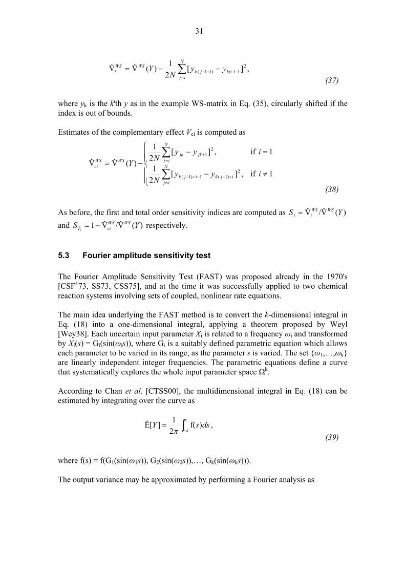
where yk is the k'th y as in the example WS-matrix in Eq. (35), circularly shifted if the index is out of bounds. Estimates of the complementary effect Vci is computed as

⎪⎪⎩

⎪⎪⎨

⎧

≠−

=−−=

∑

∑

=+−−+−

=+

N

ijijkijk

N

ijjkjk

WSWSci

iyyN

iyyNY

1if,][21

1if,][21

)(VV2

)1(1)1(

21

(38)

As before, the first and total order sensitivity indices are computed as )(V/V YS WSWSii =

and )(V/V1 YS WSWSciTi

−= respectively.

5.3 Fourier amplitude sensitivity test The Fourier Amplitude Sensitivity Test (FAST) was proposed already in the 1970's [CSF+73, SS73, CSS75], and at the time it was successfully applied to two chemical reaction systems involving sets of coupled, nonlinear rate equations. The main idea underlying the FAST method is to convert the k-dimensional integral in Eq. (18) into a one-dimensional integral, applying a theorem proposed by Weyl [Wey38]. Each uncertain input parameter Xi is related to a frequency ωi and transformed by Xi(s) = Gi(sin(ωis)), where Gi is a suitably defined parametric equation which allows each parameter to be varied in its range, as the parameter s is varied. The set ω1,…,ωk are linearly independent integer frequencies. The parametric equations define a curve that systematically explores the whole input parameter space Ωk. According to Chan et al. [CTSS00], the multidimensional integral in Eq. (18) can be estimated by integrating over the curve as

∫−=

π

ππdssY )f(

21][E ,

(39)

where f(s) = f(G1(sin(ω1s)), G2(sin(ω2s)),…, Gk(sin(ωks))). The output variance may be approximated by performing a Fourier analysis as

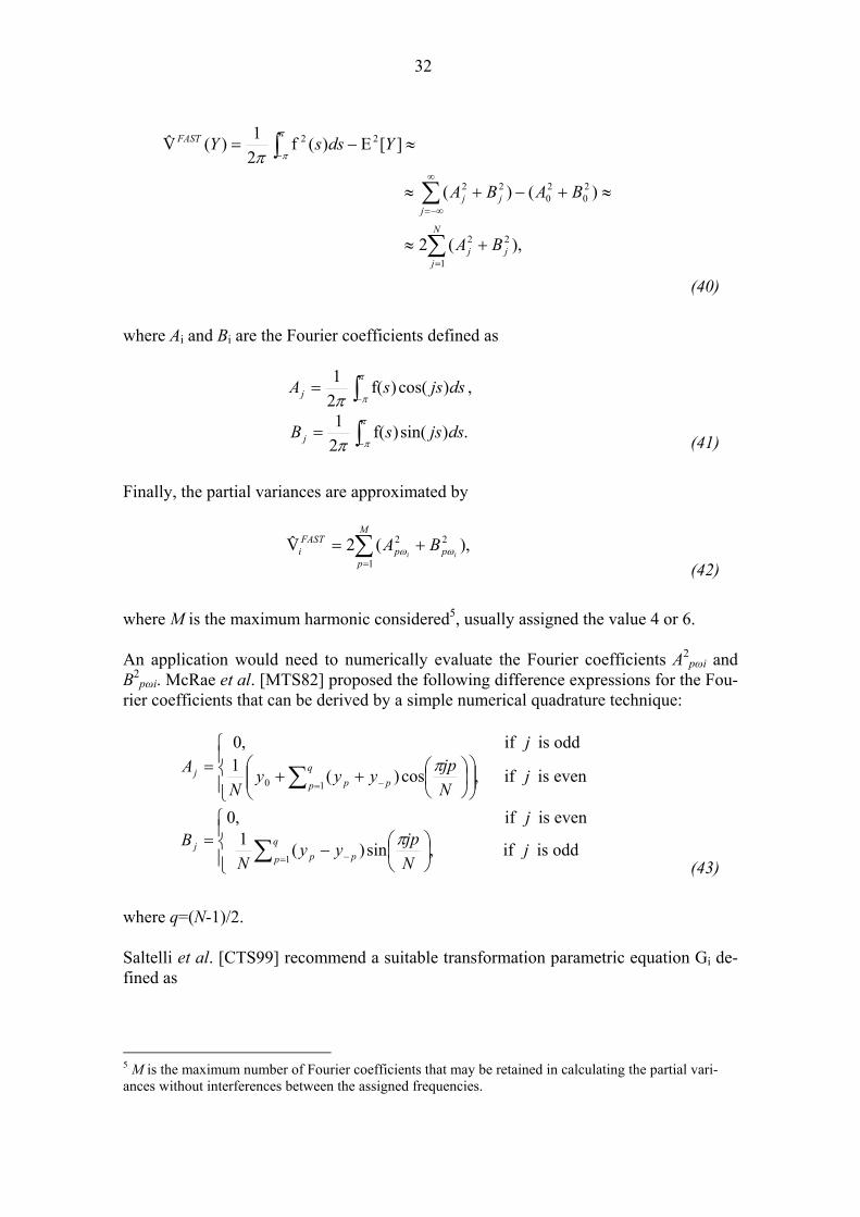
32

,)(2

)()(

][E)(f21)(V

1

22

20

20

22

22

∑

∑

∫

=

∞

−∞=

−

+≈

≈+−+≈

≈−=

N

jjj

jjj

FAST

BA

BABA

YdssYπ

ππ

(40)

where Ai and Bi are the Fourier coefficients defined as

∫−=

π

ππdsjssAj )cos()f(

21 ,

∫−=

π

ππ.)sin()f(

21 dsjssB j

(41)

Finally, the partial variances are approximated by

,)(2V1

22∑=

+=M

ppp

FASTi ii

BA ωω (42)

where M is the maximum harmonic considered5, usually assigned the value 4 or 6. An application would need to numerically evaluate the Fourier coefficients A2

pωi and B2

pωi. McRae et al. [MTS82] proposed the following difference expressions for the Fou-rier coefficients that can be derived by a simple numerical quadrature technique:

⎪⎩

⎪⎨⎧

⎟⎟⎠

⎞⎜⎜⎝

⎛⎟⎠⎞

⎜⎝⎛++= ∑ = − evenisif,cos)(1

oddisif,0

10 jNjpyyy

N

jA q

p ppj π

⎪⎩

⎪⎨⎧

⎟⎠⎞

⎜⎝⎛−= ∑ = − oddisif,sin)(1

evenisif,0

1j

Njpyy

N

jB q

p ppj π

(43)

where q=(N-1)/2. Saltelli et al. [CTS99] recommend a suitable transformation parametric equation Gi de-fined as

5 M is the maximum number of Fourier coefficients that may be retained in calculating the partial vari-ances without interferences between the assigned frequencies.

33

)).(arcsin(sin121))(sin(G)( sssX iiii ω

πω +==

(44)

According to Saltelli et al. this transformation better provides uniformly distributed samples for each parameter Xi in the unit hypercube Ωk than has been proposed by vari-ous others, among them Cukier et al. [CFS+73]. Saltelli et al. [STC99] has shown that according to the Nyquist criterion, the minimum sample size required to compute FAST

iV is 2Mωmax+1, where ωmax is the largest fre-quency in the set ω1,…,ωk. In 1998, Saltelli and Bolado [SB98] proved that the ratio )(V/V YFASTFAST

i computed with the FAST method is equivalent to the first order sensitivity indices proposed by Sobol [Sob93].

5.4 Extended Fourier amplitude sensitivity test In 1999, Saltelli et al. [STC99] proposed an improvement of the FAST method. They called it the Extended Fourier Amplitude Sensitivity Test (EFAST). With this method they could estimate the total effect indices, as in the Sobol method, by estimating the variance in the complementary set FAST

ciV . This is done by assigning a frequency ωi for the parameter Xi, usually high, and almost identical frequencies to the rest ω~i, usually low). The partial variance of the complementary set is then computed as

∑=

+=M

ppp

FASTci ii

BA1

22~~

2V ωω (45)

A modification of the parametric equation in Eq. (44) was also introduced to get a more flexible sampling scheme. Since Gi in Eq. (44) always returns exactly the same points in Ωk, a random phase-shift iϕ was added. The new equation now becomes

))(arcsin(sin121))(sin(G)( isssX iiii ϕω

πω ++== .

(46)

Because of symmetry properties, the curve now must be sampled over (-π, π). The tech-nique of using many phases generating different curves in Ωk and doing independent Fourier analysis over them and finally taking the arithmetic means over the estimates is called resampling.

34

A whole new set of model runs is needed to compute each of the k complementary vari-ances FAST

ciV , so the computational cost to obtain all first and total order indices are k(2Mωmax+1)Nr, where Nr is the number of resamples that was done.

5.5 Remarks on variance-based methods The variance-based methods described in this section are considered being quantitative sensitivity analysis methods. All methods can compute the main effect contribution of each input parameter to the output variance. The total sensitivity index can also be ob-tained by the Sobol', Jansen and EFAST methods. The total effect index is a more accu-rate measure of the influence of a parameter on the model output, since it takes into ac-count all interaction effects involving that parameter. To compute the main effect contribution, the FAST method only requires a single set of model runs. EFAST needs k(2Mωmax+1)Nr model runs to compute both the main effect as well as the total effect contribution. To compute the Sobol' indices, the required model runs are N(2k+1) using the Sobol' method and only Nk runs using the WS-sampling scheme designed to make multiple uses of the runs. Chan et al. [CTSS00] ex-pressed a concern that the reduction of model runs in Jansen's method might affect the accuracy of the obtained estimates. Quasi-random sampling has not been implemented in EIKOS, and as it is the commonly used sampling scheme in computing the Sobol' indices, the other methods might be preferable.

35

6 SUMMARY OF SENSITIVITY ANALYSIS METHODS In general, which sensitivity analysis method should be used? It depends on several pa-rameters, such as how ”heavy” the needed model computations are, the number of un-certain input parameters and whether the model output depends linearly, monotonically or non-monotonically on the input parameters under consideration. The methods for parameter screening, for example the Morris method, are useful as a first step in dealing with computationally laborious models containing large number of input parameters. The parameters that control most of the output variability can be iden-tified at low computational costs. Local sensitivity analysis is used to investigate the impact of the input parameters on the model, locally. It measures how sensitive the model is to small perturbations of the in-put parameters. When the model is nonlinear and various input parameters are affected by uncertainties of different order of magnitude, local sensitivity analysis should not be used. If the model is nonlinear, correlation and regression coefficients can not be trusted. To determine if there are nonlinearities in the model, the model coefficient of determination can be examined. A R2-value that is lower than 0.6 indicates that the regression model does not describe the dependency between the inputs and the outputs accurately enough. Another way to detect nonlinearities in the model is to examine scatter plots of the in-puts versus outputs. The coefficients computed on the basis of rank-transformed data can handle non-linear models that still are monotone. Using ranked data, the R2 value will be improved but a drawback is that the model under analysis has been altered. The analysis based on rank transformed data is more robust than for untransformed data, but for small sample sizes the results are not as trustworthy, due to loss of information from the transformation. According to Saltelli et al. [SM90] and [SH91], the most robust and reliable of the sam-pling-based methods are PRCC and SRRC. Therefore, the results obtained with these methods should be trusted more, than results obtained with other sampling-based meth-ods. Latin Hypercube sampling can be used instead of simple random sampling in the Monte Carlo analysis. Latin hypercube sampling forces the samples to be drawn from the full range of the desired distribution functions. Thus, a lower number of samples can be used to emulate the distribution functions. A drawback is that it can give a biased esti-mation of the variance of the distributions; therefore, Latin hypercube sampling should not be used to generate sample distributions used in the variance-based methods. Variance-based methods that can compute the total effect contribution of the input pa-rameters on the model output should be used if the model is thought to be non-monotone. These methods require more model evaluations, increasing with the number of input parameters, than the other methods. For models with a moderate number of in-

36

put parameters and not too long model execution time, these methods are ideal. All variance-based methods give the same type of results: first-order and total sensitivity indices. Different amount of model runs are required for the different methods. Sobol' method requires N(2k+1) model evaluations while the Jansen method only requires Nk model evaluations. For the Fourier amplitude sensitivity test the number of model evaluations required is in the order of O(k2), while for the extended version k(2Mωmax+1)Nr model evaluations are required. Drawbacks of the variance-based methods are their higher computational costs and their assumption that all information about the uncertainty in the output is captured by its variance. Overall, sensitivity analysis provides a way to identify the model inputs that have the strongest effect on the uncertainty in the model predictions. However, sensitivity analy-sis does not provide an explanation for such effects. This explanation must come from the analysts involved and, of course, be based on the mathematical properties of the model under consideration. Sensitivity analysis methods are essential tools in risk assessment and simulation modelling. Due to difficulties of implementing the methods, most sensitivity analyses are today performed using local methods, correlation or regression coefficients. The variance-based methods described here are recommended for studies of environmental risk assessment models, since these are often non-linear and can be also non-monotonic.

Figure 6.1. Flowchart of sensitivity analysis and selection of appropriate methods.

Screening, preliminary step to find the significant parameters

Model relationship is linear Model relationship is nonlin-ear but still monotonic

Spearman rank correlation coefficients

Model relationship is non-monotonic

Pearson product moment correlation coefficients

Standardized regression coefficients

Partial correlation coefficients

Standardized ranked regres-sion coefficients

Partial ranked correlation coefficients

Morris method may reduce thenumber of parameters

Fourier amplitude sensitivity test (First order index Si)

Scatter plots show relationshipbetween inputs and outputs

First and total order sensitivityindex (Si, STi)

Extended Fourier ampli-tude sensitivity test

Sobol’s Method

Jansen’s method using Winding Stairs sampling

Two-sample tests (Smirnov or Cramér-von Mises test)

37

7 EXAMPLE OF APPLICATION OF EIKOS To estimate the effect on man of radionuclide releases from a deep geological repository it is necessary to know the distribution of radionuclides in the biosphere over time. By identifying a likely release path from the discharge point, it is possible to develop a landscape model consisting of a set of linked biosphere models. Such case was imple-mented in the tool Pandora [PG+05] and sensitivity and uncertainty analyses were car-ried out with EIKOS. The objective of this example application was to study the relative performance of the different methods implemented in EIKOS for this specific type of simulation modeling problem. The model, input parameters and selected output variables used in the study are in sections 7.1, 7.2 and 7.3 respectively. The sensitivity analysis started with a screening of the input parameters (see section 3), using Morris and the Local sensitivity methods, to identify which parameters should be included in more detailed studies. Further sensitivity analyses were carried out using sampling-based (see section 4) and variance-based methods (see section 5) in order to compare the performance of the different methods available in EIKOS.

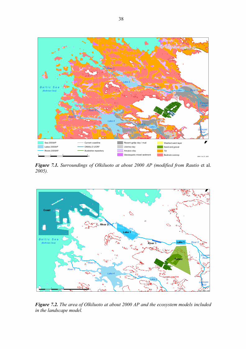
7.1 The landscape model used in the study The model describes the future terrain and ecosystem development on the basis of sea depth data and on the approximation that 2000 years after present there will be a land uplift of 10 meters above the current depth and elevation values (Rautio et al. 2005). It was assumed that there will be no significant sea level changes during this period. The discharge was assumed to go directly to an area above the repository, which at the time will be covered by forest. The succession of linked biosphere models was identified from maps of the terrain and will also involve lakes, rivers and coastal areas, as illus-trated in figure 7.1. From the depressions remaining under the sea level, locations of lakes can be estimated. Likely some of the lakes will be larger, or smaller, than the depression, but for testing the tools and modelling methods these estimates were judged to be adequate. Based on the type of current sea bottom sediments (Fig. 7.1), future forest types on the area can be forecasted [RAI05]. The current prevailing forest types will prevail also in the future, but somewhat more wetlands and deciduous forests around the water bodies are predicted. On the basis of the terrain and ecosystems forecast for the selected time period the cor-responding landscape model (Fig. 7.2) was built using ecosystem-specific biosphere modules taken from earlier assessments and modelling exercises (see Appendices 1-4). A view of the implementation in Pandora [PG+05] of the interlinked ecosystem models is shown in Fig. 7.3.

38

´0 2 41

km ARIK / Oct 27, 2005

B a l t i c S e a(Bothnian Sea)

Lake 2

Lake 1River 1

River 2

Lake 4

Lake 3River 3

River 4

River 5

River 0

EurajokiRiver

LapinjokiRiver

Sea 2000AP

Lakes 2000AP

Rivers 2000AP Illustrative repository

Current coastline

ONKALO UCRF

Washed sand layer

Sand and gravel

Till

Bedrock outcrop

Recent gyttja clay / mud

Litorina clay

Glaciaquatic mixed sediment

Ancylus clay

Figure 7.1. Surroundings of Olkiluoto at about 2000 AP (modified from Rautio et al. 2005).

Coast

Forest

Lake 1

Lake 1River 1

River 2

´

0 2 41km

ARIK / Oct 27, 2005

B a l t i c S e a(Bothnian Sea)

Lake 4

Lake 3River 3

River 4

River 5

River 0

EurajokiRiver

LapinjokiRiver

Current coastline

Figure 7.2. The area of Olkiluoto at about 2000 AP and the ecosystem models included in the landscape model.

39

in soluble

conc water

out souluble

River2

in soluble

conc water

out souluble

River1

Cl-36 301000 Cs-137 30

I-129 15700000Ni-59 76000 Pu-239 24110 Ra-226 1600 Tc-99 211000

PANDORA

influx soluble

backflux soluble

conc water

Outer Coast

influx water

outflux water

conc water

Lake2

influx water

outflux water

conc water

Lake1

influx soluble

outflux soluble

conc water

Inner Coast

In1

conc soil

outflux

Forest

C_River2

C_River2

C_River1

C_River1

C_OuterCoas

C_OuterCoast

C_Lake2

C_Lake2

C_Lake1

C_Lake1

C_InnerCoas

C_InnerCoast

C_Forest

C_Forest-C-

1 Bq/Yr Input

Figure 7.3 The landscape model implemented in Pandora, the main level view.

The ecosystem models included in the landscape model were:

• a coast model taken from [KB00], see Appendix 1. • a lake model taken from [KB00], see Appendix 2, • a river model taken from [JE05], see Appendix 3, • a forest model taken from [Avi06], see Appendix 4

7.2 Input parameters The parameters of the landscape model were divided into three types: radionuclide spe-cific (for example the distribution coefficients (Kd) and the soil-to-plant concentration ratios CR), object specific and system specific. Object specific parameters are parame-ters that have specific values for each particular object, such as the mean depth of a lake. System specific parameters are parameters that have the same value for all objects of the same type.

40

The probability density functions assigned to the parameters (see Tables 7.1-7.3) were taken from [KB00], except for the parameters of the forest model, which were taken from [Avi06] and the parameters of the river model, which were taken from [JE05]. All parameters were assigned the used triangular distribution, and the distributions are specified by minimum, mode (most probable) and maximum values. Note that not much attention was given to the uncertainty in the parameter data since the goal was to test EIKOS performance, and get some first impressions of a real-case use of the tool on a landscape model.

7.3 The studied output variables The model supports calculations of time-dependent inventories and concentrations of multiple radionuclides in several environmental media of the objects included in the landscape (see Figure 7.3). For sensitivity analysis three output variables were consid-ered: • The Cl-36 concentration in the soil of the forest ecosystem after 1000 years of con-

tinuous release of 1 Bq/y into the forest. • The Cl-36 concentration in the water of Lake 2 after 1000 years of continuous re-

lease of 1 Bq/y into the forest. • The Cl-36 concentration in the water of outer coast after 1000 years of continuous

release of 1 Bq/y into the forest. Table 7.1 The object-specific parameters used in the simulations. “GIS” refers to data acquired from the geographical information described in section 7.1. Parameter Name in model Unit Min Mode Max Ref. Forest area area_Forest m2 5,0E+05 2,2E+06 4,4E+06 GIS Forest catchment area Acatch_Forest m2 2,5E+05 4,4E+06 7,0E+06 GIS Bulk density of forest soil density_soil Kg/m3 7,0E+02 1,2E+03 1,5E+03 [Avi06] Thickness of forest soil rooting layer h M 0.2 0.3 0.5 [Avi06] Yearly production of tree leaves LP Kg dw/m2/yr 0.05 0.08 1.7 [Avi06] Yearly production of understorey plants UP Kg dw/m2/yr 0.02 0.08 0.25 [Avi06] Yearly production of tree wood WP Kg dw/m2/yr 0.018 0.18 1.8 [Avi06] Average tree lifetime Tlife Year 2,0E+01 4,0E+01 6,0E+01 [Avi06] Volumetric water content in soil theta m3/m3 0.1 0.2 0.5 [Avi06] Average depth of river 1 R1_Depth M 0.1 0.3 1,0E+00 GIS Length of river 1 R1_deltax M 1,0E+02 4,1E+02 1,5E+03 GIS Average depth of river 2 R2_Depth M 0.1 0.3 1,0E+00 GIS Length of river 2 R2_deltax M 6,7E+01 1,7E+03 2,9E+03 GIS Area of inner coast area_InnerCoast m2 1,0E+08 2,0E+08 3,0E+08 GIS Average depth of inner coast IC_D M 2.5 3,0E+00 3.5 [KB00] Area of outer coast area_OuterCoast M2 2,0E+11 2,3E+11 2,6E+11 GIS Average depth of outer coast OC_D M 6,0E+00 7,0E+00 8,0E+00 [KB00] Yearly average flowrate of Eurajoki River Flowrate_Eurajoki m3/yr 2,0E+08 3,0E+08 4,0E+08 GIS Area of lake 1 L1Area m2 2,6E+05 8,6E+05 1,3E+06 GIS Average depth of lake 1 L1D M 0.1 0.3 0.9 [KB00] Area of lake 2 L2Area m2 5,0E+04 1,4E+05 2,2E+05 GIS Average depth of lake 2 L2D M 0.1 0.3 0.6 [KB00]

41

Table 7.2 The system-specific parameters used in the simulations. Parameter Name in model Unit Min Mode Max Ref. Plant biomass in rivers M_biomass Kg·fw/m2 4,0E+00 5,0E+00 6,0E+00 [JE05] Cross-sectional angle in rivers Alpha Rad 0.5 0.7 0.9 [JE05] Diffusion coefficient in rivers D m2/yr 0.0079 0.0158 0.0237 [JE05] Particle size distribution, rivers (50% percentile)

D_50 m 0.0005 0.0007 0.0009 [JE05]

Particle size distribution, rivers (90% percentile)

D_90 m 0.0017 0.0019 0.0021 [JE05]

Resuspension of surface sediment (coast)

Resusp Year-1 0.1 0.2 0.3 [KB00]

Water retention time, inner coast RetTime_IC Year 0.0014 0.002 0.0027 [KB00] Specific density in rivers S [-] 2.4 2.6 2.8 [JE05] Gross sedimentation rate, inner coast SR_Coast Kg·dw/(m2·yr) 0.5 1.1 1.5 [KB00] Gross sedimentation rate, outer coast SR_Sea Kg·dw/(m2·yr) 0.05 0.2 0.4 [KB00] Gross sedimentation rate, lakes SR_lake Kg·dw/(m2·yr) 0.5 1.1 1.5 [KB00] Suspended matter, inner coast Susp_Coast Kg·dw/m3 0.003 0.009 0.03 [KB00] Suspended matter, outer coast Susp_Sea Kg·dw/m3 0.0005 0.001 0.002 [KB00] Suspended matter, lakes Susp_lake Kg·dw/m3 0.005 0.01 0.06 [KB00] Sedimentation velocity in rivers V_partsed m/yr 3,0E+02 4,0E+02 5,0E+02 [JE05] Advective transport velocity in bed siediment

Vz m/yr 157.68 315.36 473.04 [JE05]

Suspended particulate matter in stream water

cp Kg/m3 0.01 0.02 0.03 [JE05]

Depth of surface sediment in rivers deltaz1 m 0.25 0.5 0.75 [JE05] Depth of deep sediment in rivers deltaz2 m 0.25 0.5 0.75 [JE05] Sediment porosity in rivers porosity_sed [-] 0.7 0.8 0.9 [JE05] Sediment density in rivers rho_sed Kg/m3 7,0E+02 1,1E+03 1,5E+03 [JE05] Dry mass of surface sediment, inner coast

rho_sed_Sea Kg/m2 5,0E+00 1,0E+01 1,5E+01 [KB00]

Table 7.3 The radionuclide-specific parameters used in the simulations. Parameter Name in model Unit Min Mode Max Ref. Half-time to reach sorption equilib-rium

Tk Year 0.0005 0.001 0.0015 [JE05]

Bioconcentration factor BCF[Cl-36] (Bq/kg·fw)/(Bq/l)

1,0E+02 2,0E+02 3,0E+02 [JE05]

Conc. ratio of nuclide from soil to tree leaves

CR_L[Cl-36] [-] 0.8 1,0E+01 2,8E+01 [Avi06]

Conc. ratio of nuclide from soil to understorey plants

CR_U[Cl-36] [-] 3,0E+00 2,8E+01 1,7E+02 [Avi06]

Conc. ratio of nuclide from soil to tree wood

CR_W[Cl-36] [-] 0.8 3,0E+00 1,1E+01 [Avi06]

Distribution coefficient in sediment in rivers

KB[Cl-36] m3/kg 0.003 0.03 0.3 [JE05]

Distribution coefficient in stream water

Kd[Cl-36] m3/kg 0.03 0.3 3,0E+00 [KB00]

Distribution coefficient, lakes Kd_lake[Cl-36] m3/kg 0.1 1,0E+00 1,0E+01 [KB00]

Distribution coefficient soil Kd_soil[Cl-36] m3/kg 0.0001 0.001 0.01 [KB00]

42

7.4 Results of the sensitivity and uncertainty analysis 7.4.1 Results of screening study The Morris method was used to screen out the parameters with negligible influence on the outputs. The total number of realisations was 13750 and the quantiles of the distri-butions were used to define the p levels among which each input parameter was varied. The results obtained with the Morris method for the three studied outputs are shown in figures 7.4-7.6. In addition to the Morris method, local sensitivity indexes were calculated for screening out unimportant parameters. These were obtained by varying each parameter by 5% of its nominal value. The results from the local method for the three studied outputs are shown in figures 7.7-7-9. It can be seen that the Local method only shows the parameters that are indicated as the most significant by the Morris method as significant. The parameters indicated by the Local method as significant are however coherent with the results from the Morris method, and no additional parameters are indicated as important. The results of the Morris and the Local screening methods are given in Table 7.4, listing the parameters that were indicated as important for the selected outputs, in ranked order (constituting totally 9 unique parameters of the model).

Figure 7.4 The results of the Morris method for the concentration of Cl-36 in forest soil.

0 1 2 3 4 5 6

x 10-9

0

0.2

0.4

0.6

0.8

1

1.2

1.4

1.6x 10-9

Estimated means (µ)

Sta

ndar

d D

evia

tions

( σ)

Estimated means and standard deviations of elementary effects, for output ConcForest

Acatch Forest

Kd soil

43

Figure 7.5 The results of the Morris method for the concentration of Cl-36 in the water of Lake 2.

Figure 7.6 The results of the Morris method for the concentration of Cl-36 in the water of the outer coast area.

0 0.5 1 1.5 2 2.5 3 3.5 4 4.5 5

x 10-10

0

1

2

3

4

5

6

7

8x 10-11

Estimated means (µ)

Sta

ndar

d D

evia

tions

( σ)

Estimated means and standard deviations of elementary effects, for output ConcLake

Flowrate Eurajoki

Kd_soil, WP,

Acatch_Forest, CR_W,

Area_Forest

0 1 2 3 4 5 6 7 8

x 10-16

0

0.2

0.4

0.6

0.8

1

1.2x 10-16

Estimated means (µ)

Sta

ndar

d D

evia

tions

( σ)

Estimated means and standard deviations of elementary effects, for output ConcCoast

OC_D

area_OuterCoast

Kd Soil, Acatch_Forest,

WP, CR_W,

area_Forest, Tlife

44

Figure 7.7. The local sensitivity indices for the concentration of Cl-36 in the forest soil .

Figure 7.8 The local sensitivity indices for the concentration of Cl-36 in water of Lake 2.

-1 -0.8 -0.6 -0.4 -0.2 0 0.2 0.4 0.6 0.8 1

WP

Acatch Forest

Kd soil

area Forest

Flowrate Eurajoki

local on output ConcLake

-1 -0.8 -0.6 -0.4 -0.2 0 0.2 0.4 0.6 0.8 1

CR W

WP

area Forest

Kd soil

Acatch Forest

local on output ConcForest

45

Figure 7.9 The local sensitivity indices for the concentration of Cl-36 in water of the outer coast area.

Table 7.4 The most influential parameters as indicated by the screening methods. Output: Parameters: Conc. In forest soil 1) Forest catchment area (‘Acatch_Forest’)

2) Distribution coefficient soil (‘Kd_Soil’)

Conc. In lake water 1) Yearly average flowrate of Eurajoki River (‘Flowrate_Eurajoki’) 2) Distribution coefficient soil (‘Kd_Soil’) 3) Yearly production of tree wood (‘WP’) 4) Forest catchment area (‘Acatch_Forest’) 5) Conc. ratio of nuclide from soil to tree wood (‘CR_W’) 6) Forest area (‘area_Forest’)

Conc. In coast water 1) Average depth of outer coast (‘OC_D’) 2) Area of outer coast (‘area_OuterCoast’) 3) Distribution coefficient soil (‘Kd_Soil’) 4) Forest catchment area (‘Acatch_Forest’) 5) Yearly production of tree wood (‘WP’) 6) Conc. ratio of nuclide from soil to tree wood (‘CR_W’) 7) Forest area (‘area_Forest’) 8) Average tree lifetime (‘Tlife’)

-1 -0.8 -0.6 -0.4 -0.2 0 0.2 0.4 0.6 0.8 1

Acatch Forest

Kd soil

area Forest

OC D

area OuterCoast

local on output ConcCoast

46

7.4.2 Results of the sampling based methods A total of 10000 simulations were carried out with samples from all parameters gener-ated using Latin Hypercube Sampling. LHS evaluations are presented in figures 7.16-7.24. They are further discussed together with the results from other methods in section 7.4.4 below. In figures 7.20, 7.22 and 7.24, the data plotted are the ranked values. It is worth noticing that in all applied methods, the whole set of parameters listed in ta-bles 7.1-7.3 were used, to be able to study how the results compare with the screening methods. In a real assessment, only the nine most influential parameters from table 7.4 might have been used for further analysis.

Figure 7.16 Histogram-plot from EIKOS showing the distribution of the concentration of Cl-36 in forest soil (at t=1000 years).

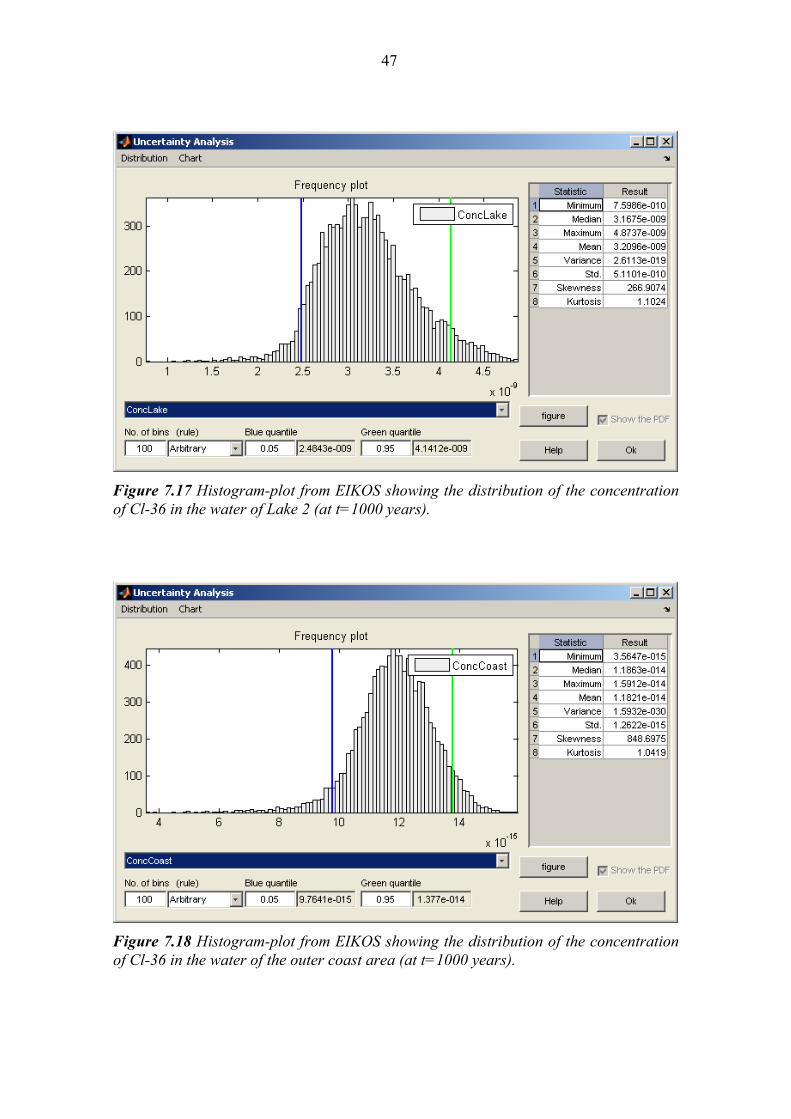
47

Figure 7.17 Histogram-plot from EIKOS showing the distribution of the concentration of Cl-36 in the water of Lake 2 (at t=1000 years).

Figure 7.18 Histogram-plot from EIKOS showing the distribution of the concentration of Cl-36 in the water of the outer coast area (at t=1000 years).

48

-1 -0.8 -0.6 -0.4 -0.2 0 0.2 0.4 0.6 0.8 1

CR W

theta

WP

Acatch Forest

Kd soil

SRRC on output ConcForest

Figure 7.19 Sensitivity indices (using SRRC) for the concentration of Cl-36 in the forest soil

.

1000 2000 3000 4000 5000 6000 7000 8000 9000 10000

1000

2000

3000

4000

5000

6000

7000

8000

9000

10000

ConcForest

Kd soil

Figure 7.20 The concentration of Cl-36 in the forest soil vs. Kd_Soil.

49

-1 -0.8 -0.6 -0.4 -0.2 0 0.2 0.4 0.6 0.8 1

CR W

Acatch Forest

Kd soil

WP

Flowrate Eurajoki

SRRC on output ConcLake

Figure 7.21 Sensitivity indices (using SRRC) for the concentration of Cl-36 in the water of Lake 2.

1000 2000 3000 4000 5000 6000 7000 8000 9000 10000

1000

2000

3000

4000

5000

6000

7000

8000

9000

10000

ConcLake

Flowrate Eurajoki

Figure 7.22 The concentration of Cl-36 in the water of Lake 2 vs. the Eurajoki flowrate.

50

-1 -0.8 -0.6 -0.4 -0.2 0 0.2 0.4 0.6 0.8 1

CR W

Kd soil

WP

area OuterCoast

OC D

SRRC on output ConcCoast

Figure 7.23 Sensitivity indices (using SRRC) for the concentration of Cl-36 in the water of the outer coast area.

1000 2000 3000 4000 5000 6000 7000 8000 9000 10000

1000

2000

3000

4000

5000

6000

7000

8000

9000

10000

ConcCoast

area OuterCoast

Figure 7.24 The concentration of Cl-36 in the water of the outer coast area vs. the outer coast mean depth.

51

7.4.3 Results of the Variance based methods The results of the EFAST evaluations are presented in figures 7.25-7.27. They are fur-ther discussed together with the results from other methods in section 7.4.4 below. A total of 8946 model evaluations were performed. The results of the Sobol evaluations are presented in figures 7.28-7.30. They are further discussed together with the results from other methods in section 7.4.4 below. A total of 10000 model evaluations were performed. The results of the Jansen evaluations are presented in figures 7.31-7.33. They are further discussed together with the results from other methods in section 7.4.4 below. A total of 9000 model evaluations were performed.

0 0,2 0,4 0,6 0,8

OC_D

area Forest

Flowrate_Eurajoki

Tlife

WP

CR_W

area_OuterCoast

Kd_soil

Acatch_Forest

TSI on output ConcForest

Figure 7.25 Total sensitivity indices (using EFAST) for the concentration of Cl-36 in forest soil.

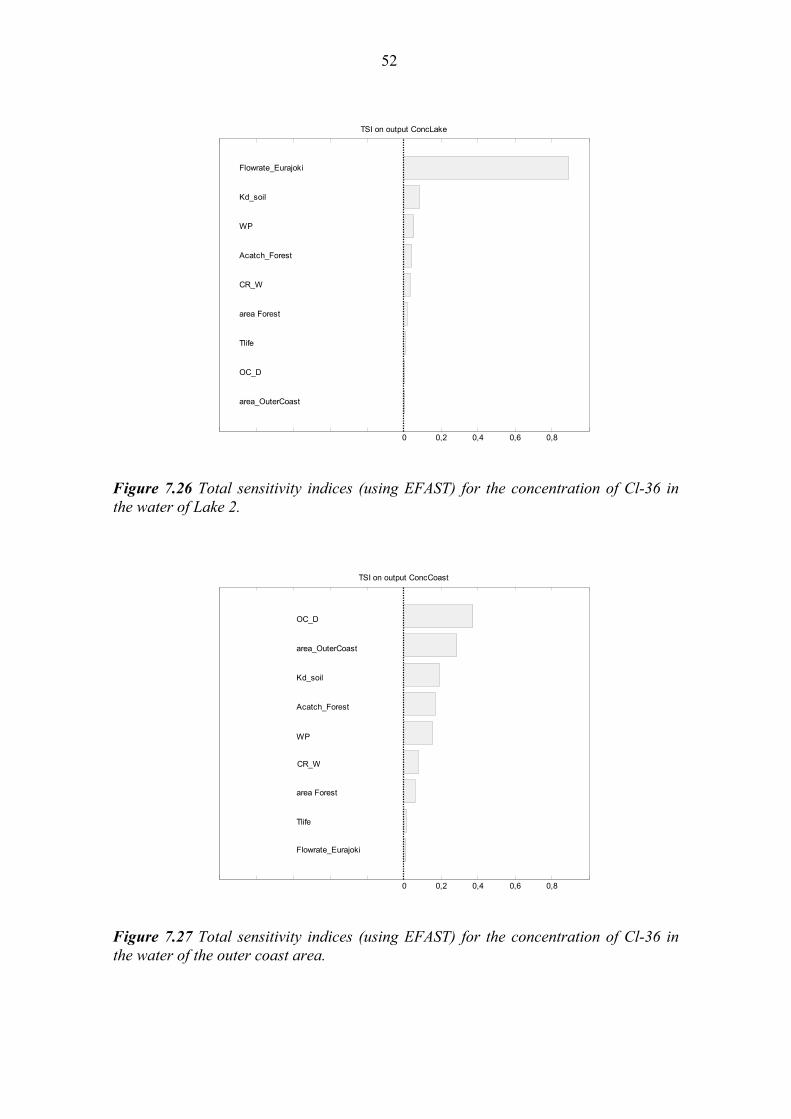
52

0 0,2 0,4 0,6 0,8

area_OuterCoast

OC_D

Tlife

area Forest

CR_W

Acatch_Forest

WP

Kd_soil

Flowrate_Eurajoki

TSI on output ConcLake

Figure 7.26 Total sensitivity indices (using EFAST) for the concentration of Cl-36 in the water of Lake 2.

0 0,2 0,4 0,6 0,8

Flowrate_Eurajoki

Tlife

area Forest

CR_W

WP

Acatch_Forest

Kd_soil

area_OuterCoast

OC_D

TSI on output ConcCoast

Figure 7.27 Total sensitivity indices (using EFAST) for the concentration of Cl-36 in the water of the outer coast area.

53

-1 -0.8 -0.6 -0.4 -0.2 0 0.2 0.4 0.6 0.8 1

area_OuterCoast

OC_D

Flowrate_Eurajoki

area Forest

Tlife

WP

CR_W

Kd_soil

Acatch_Forest

TSI on output ConcForest

Figure 7.28 Total sensitivity indices (using Sobol) for the concentration of Cl-36 in the forest soil.

-1 -0.8 -0.6 -0.4 -0.2 0 0.2 0.4 0.6 0.8 1

area_OuterCoast

OC_D

Tlife

CR_W

area Forest

Acatch_Forest

WP

Kd_soil

Flowrate_Eurajoki

TSI on output ConcLake

Figure 7.29 Total sensitivity indices (using Sobol) for the concentration of Cl-36 in the water of Lake 2.

54

0 0,2 0,4 0,6 0,8

Flowrate_Eurajoki

Tlife

areaForest

CR_W

WP

Kd_soil

Acatch_Forest

area_OuterCoast

OC_D

TSI on output ConcCoast

Figure 7.30 Total sensitivity indices (using Sobol) for the concentration of Cl-36 in the water of the outer coast area.

0 0,2 0,4 0,6 0,8

area_OuterCoast

OC_D

Flowrate_Eurajoki

Tlife

area Forest

CR_W

WP

Kd_soil

Acatch_Forest

TSI on output ConcForest

Figure 7.31 Total sensitivity indices (using Jansen) for the concentration of Cl-36 in the forest soil.

55

0 0,2 0,4 0,6 0,8

area_OuterCoast

OC_D

Tlife

area Forest

CR_W

Acatch_Forest

WP

Kd_soil

Flowrate_Eurajoki

TSI on output ConcLake

Figure 7.32 Total sensitivity indices (using Jansen) for the concentration of Cl-36 in the water of Lake 2.

0 0,2 0,4 0,6 0,8

Flowrate_Eurajoki

Tlife

area Forest

CR_W

WP

Kd_soil

Acatch_Forest

area_OuterCoast

OC_D

TSI on output ConcCoast

Figure 7.33 Total sensitivity indices (using Jansen) for the concentration of Cl-36 in the water of the outer coast area.

56

7.4.4 Conclusions of the sensitivity analysis The results obtained with the different sensitivity analysis methods used are summa-rized in tables 7.5-7.7. The quantitative contribution of the parameters to the output variance is given in percentages (for the variance based methods). The parameters con-tributing less than 2 % were not included in the tables. The distribution coefficient in forest soil and the catchment area of the forest are the overall dominating parameters for the concentration in the forest soil. It can be seen from Table 7.5 that the order of importance of the distribution coefficient and catchment area are reversed for the sampling based method (with Latin Hypercube Sampling), al-though the difference between them is small, as shown by the variance-based methods. For the variance-based methods, the agreement is very good, with the minor difference being that EFAST indicates a somewhat lower overall contribution to the output vari-ance. It was realized during the calculations that when EFAST is applied to models with many input parameters, the noise level is high compared to the methods of Sobol and Jansen. This explains why the area of the outer coast contributes (3%) to the uncertainty of the estimate of the concentration in forest soil. As the area of the outer coast cannot influence at all on the concentration in soil, this result indicates that the noise level of EFAST is higher than for the other methods. This is probably caused by the presence of interference in the sampling scheme of EFAST, and should be further investigated. From Table 7.6 it can be seen that the overall agreement between methods is also very good for the concentration in water of Lake 2, but still the noise-level for EFAST is somewhat high. For the concentration in the water of Lake 2, the flow rate of the Eura-joki River is totally dominating. This is expected since the only release of radionuclides into the water of Lake 2 is directly from the forest, and the flow rate of the Eurajoki River, used to calculate the water retention time in the lake, is much higher than the run-off from the surrounding catchment areas of Lake 2. Table 7.5 Ranking of the parameters with significant influence on the concentration in the Forest soil by the different SA methods used. Sampling based (LHS) EFAST Sobol Jansen Kd soil Acatch Forest [44%] Acatch Forest [52%] Acatch Forest [51%] Acatch Forest Kd soil [42%] Kd soil [44%] Kd soil [45%] - area_OuterCoast

[3%] - -

Table 7.6 Ranking of the parameters with significant influence on the concentration in the water of Lake 2 by the different SA methods used. Probabilistic (LHS) EFAST Sobol Jansen Flowrate Eurajoki Flowrate Eurajoki

[78%] Flowrate Eurajoki [77%]

Flowrate Eurajoki [73%]

WP Kd soil [7%] Kd soil [11%] Kd soil [7%] Kd soil WP [5%] WP [5%] WP [7%] Acatch Forest Acatch Forest [3%] Acatch Forest [4%] Acatch Forest [7%] CR_W CR_W [3%] - CR_W [4%]

57

Table 7.7 Ranking of the parameters with significant influence on the concentration in the water of the outer coast by the different SA methods used. Probabilistic (LHS) EFAST Sobol Jansen OC_D OC_D [28%] OC_D [28%] OC_D [26%] area_OuterCoast area_OuterCoast [21%] area_OuterCoast [26%] area_OuterCoast [21%]WP Kd soil [14%] Acatch Forest [11%] Acatch Forest [14%] Kd soil Acatch Forest [13%] Kd soil [11%] Kd soil [14%] CR_W WP [12%] WP [8%] WP [13%] - CR_W [6%] CR_W [8%] CR_W [8%] - area Forest [5%] area Forest [6%] area Forest [4%] The concentration in the water of the outer coast is the only output that can be depend-ant on any parameter of the model, since the radionuclides flow directly with water from the release point in the forest to the coast, via the network of rivers and lakes. This explains why a larger number of parameters contribute to this output (Table 7.7). Yet, almost perfect agreement is obtained between the variance based methods. Improvements to the results could be made by increasing the number of total model evaluations for the different methods used, thereby minimizing any statistical error in-troduced. Still, the obtained correlation between the screening methods and the sam-pling- and variance-based methods was very good. The Morris method has shown being a very robust screening method, and therefore the results could be improved by applying the variance based methods only to those pa-rameters indicated by Morris as important. This is because the parameters that are not indicated as important by the Morris method will only increase the overall statistical noise level in the variance based methods. Further, in this test case no selective mapping was made between input parameters and outputs, meaning that the analyses included irrelevant parameters for several model out-puts (for instance the area of the outer coast was considered in the SA for the concentra-tion in the forest soil). Had such a selective mapping been made, the noise-level might have been lower and the results, especially for the EFAST method, would have been better.

58

59

8 CONCLUDING REMARKS Overall, sensitivity analysis provides a way to identify the model inputs that have the strongest effect on the uncertainty in the model predictions. However, sensitivity analy-sis does not provide an explanation for such effects. This explanation must come from the analysts involved and, of course, be based on the mathematical properties of the model under consideration. Sensitivity analysis methods are essential tools in risk assessment and simulation modelling. Due to difficulties of implementing the methods, most sensitivity analyses are today performed using local methods, correlation or regression coefficients. The variance-based methods described here are recommended for studies of environmental risk assessment models, since these are often non-linear and can be also non-monotonic. The test application has shown that EIKOS is an easy to use and robust tool for performing SA studies of models developed with Pandora. For this test, the model created in Pandora was simply loaded into EIKOS, and all SA and simulation settings, as well as the parameter management, was handled from within EIKOS. A full assessment could also be saved from within EIKOS and later opened to reproduce the results. Also the landscape modelling procedure was found technically feasible and the work-flow combining Pandora and EIKOS seen well controlled, although some streamlining is recommended in future.

60

61

REFERENCES [Avi06] R. Avila. Model of the long-term transfer of radionuclides in forest. Svensk Kärnbränslehantering Ab, SKB Technical report, in print. [CFS73] R. I. Cukier, C. M. Fortuin, Kurt E. Shuler, A. G. Petschek, and J. H. Schaibly. Study of the sensitivity of coupled reaction systems to uncertainties in rate coefficients. I theory. The Journal of Chemical Physics, 59(8):3873–3878, October 1973. [Con99] William Jay Conover. Practical Nonparametric Statistics. John Wiley & Sons, Inc., 3rd edition, 1999. [CSS75] R. I. Cukier, J. H. Schaibly, and Kurt E. Shuler. Study of the sensitivity of coupled reaction systems to uncertainties in rate coefficients. III analysis of the ap-proximations. The Journal of Chemical Physics, 63(3):1140–1149, August 1975. [CST00] Karen Chan, Andrea Saltelli, and Stefano Tarantola. Winding stairs: A sam-pling tool to compute sensitivity indices. Statistics and Computing, 10(3):187–196, July 2000. [CTSS00] Karen Chan, Stefano Tarantola, Andrea Saltelli, and Ilya M. Sobol0. Vari-ance-based methods. In Sensitivity analysis, Wiley Ser. Probab. Stat., pages 167–197. Wiley, Chichester, 2000. [HS96] Toshimitsu Homma and Andrea Saltelli. Importance measure in global sensitiv-ity analysis of nonlinear models. Reliability Engineering and System Safety, 52(1):1–7, 1996. [IC82] Ronald L. Iman and W. J. Conover. A distributionfree approach to inducing rank correlation among input variables. Communications in Statistics: Simulation and Com-putations, 11(3):311–334, 1982. [JE05] Jonsson, K. and Elert, M. Model for radionuclide transport in running waters. Svensk Kärnbränslehantering Ab, SKB TR 05-03. [JRD94] M.J.W. Jansen, W.A.H. Rossing, and R.A. Daamen. Monte Carlo estimation of uncertainty contributions from several independent multivariate sources. Predictabil-ity and Nonlinear Modelling in Natural Sciences and Economics, pages 334–343, 1994. [KB00] Karlsson, S. and Bergström, U. Dose rate estimates for the Olkiluoto site using the biospheric models of SR 97. Posiva Working report 2000-20. [Mor91] Max D. Morris. Parameterial sampling plans for preliminary computational experiments. Technometrics, 33(2):161–174, May 1991.

62

[MTS82] Gregory J. McRae, James W. Tilden, and John H. Seinfeld. Global sensitivity analysis - a computational implementation of the Fourier amplitude sensitivity test (FAST). Computers and Chemical Engineering, 6(1):15–25, 1982. [PG05] Åstrand, P-G., Jones, J., Broed, R. & Avila, R. Pandora technical description and user guide. Posiva Working report 2005-64. [RAI05] Rautio, P., Aro, L. & Ikonen, A. T. K. Terrain development at Olkiluoto site and implications to biosphere assessment. Proceedings of the 2nd International Confer-ence on Radioactivity in the Environment, Nice, October 2-6, 2005. Norwegian Radia-tion Protection Authority (printed by). pp. 372-375. [Sal00] Andrea Saltelli. What is sensitivity analysis? In Sensitivity analysis, Wiley Ser. Probab. Stat., pages 3–13. Wiley, Chichester, 2000. [SB98] Andrea Saltelli and Ricardo Bolado. An alternative way to compute Fourier am-plitude sensitivity test (FAST). Computational Statistics and Data Analysis, 26:445–460, 1998. [SH91] Andrea Saltelli and T Homma. Lisa package user’s guide, part III: SPOP (Sta-tistical POst Processor) uncertainty and sensitivity analysis for model output program description and user guide. Technical report, CEC/JRC Nuclear Science and Technol-ogy, 1991. [SM90] Andrea Saltelli and J Marivoet. Non-parametric statistics in sensitivity analysis for model output: A comparison of selected techniques. Reliability Engineering and System Safety, 28:229–253, 1990. [Sob93] I. M. Sobol0. Sensitivity analysis for nonlinear mathematical models. Mathe-matical Modeling and Computational Experiment, 1(4):407–414, 1993. [Sob01] I. M. Sobol0. Global sensitivity indices for nonlinear mathematical models and their Monte Carlo estimates. Math. Comput. Simulation, 55(1-3):271–280, 2001. The Second IMACS Seminar on Monte Carlo Methods (Varna, 1999). [SS73] J. H. Schaibly and Kurt E. Shuler. Study of the sensitivity of coupled reaction systems to uncertainties in rate coefficients. II applications. The Journal of Chemical Physics, 59(8):3879–3888, October 1973. [STC99] Andrea Saltelli, Stefano Tarantola, and Karen Chan. A quantitative model-independent method for global sensitivity analysis of model output. Technometrics, 41(1):39–56, February 1999. [STCR04] Andrea Saltelli, Stefano Tarantola, Francesca Campolongo, and Marco Ratto. Sensitivity analysis in practice. John Wiley & Sons Ltd., Chichester, 2004. A guide to assessing scientific models.

63

[Wey38] H. Weyl. Mean motion. American Journal of Mathematics, 60(4):889–896, October 1938.

64

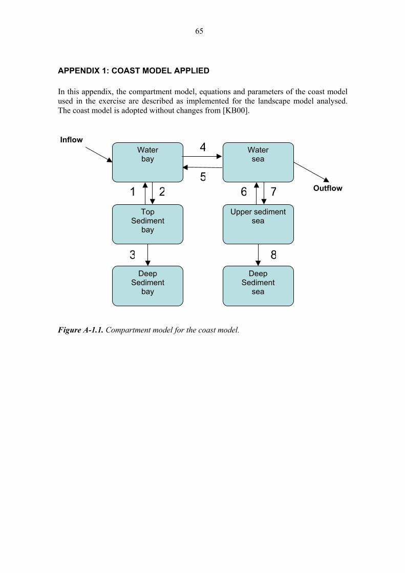
65

APPENDIX 1: COAST MODEL APPLIED In this appendix, the compartment model, equations and parameters of the coast model used in the exercise are described as implemented for the landscape model analysed. The coast model is adopted without changes from [KB00].

Figure A-1.1. Compartment model for the coast model.

Water bay

Top Sediment

bay

Deep Sediment

bay

Water sea

Upper sediment sea

Deep Sediment

sea

Inflow

Outflow1 2

3

4

56 7

8

66

Table A-1.1. Equations used in the coast model.

Transfer Nr.: Transfer Coefficient (Bq/Yr): 1, 6

sedρResusp

2, 7

)1( SuspKdDSRKd⋅+⋅

⋅

3, 8

sedρResuspSR −

4

tTimeRe1

5

Sea

bay

VV

⋅tTimeRe1

Table A-1.2. Parameters used in the coast model.

Parameter Name Description Resusp Resuspended fraction

sedρ Mass of upper sediment

Kd Distribution factor SR Gross sediment rate D Mean depth Susp Concentration of suspended matter in water RetTime Retention Time for inner coast water (bay)

SeaV Water volume of sea (outer coast)

bayV Water volume of bay (inner coast)

67

APPENDIX 2: LAKE MODEL APPLIED In this appendix, the compartment model, equations and parameters of the lake model used in the exercise are described as implemented for the landscape model analysed. The lake model is adopted without changes from [KB00].

Figure A-2.1. Compartment model for the lake model.

Water

Top Sediment

Deep Sediment

Inflow Outflow

1 2

3

4

68

Table A-2.1. Equations used in the lake model.

Transfer Nr.: Transfer Coefficient (Bq/Yr): 1

sedρResusp

2

)1( SuspKdDSRKd⋅+⋅

⋅

3

sedρResuspSR −

4

tTimeRe1

Table A-2.2. Parameters used in the lake model.

Parameter Name Description Resusp Resuspended fraction

sedρ Mass of upper sediment

Kd Distribution factor SR Gross sedimentation rate D Mean depth Susp Concentration of suspended matter in water RetTime Retention time in lake

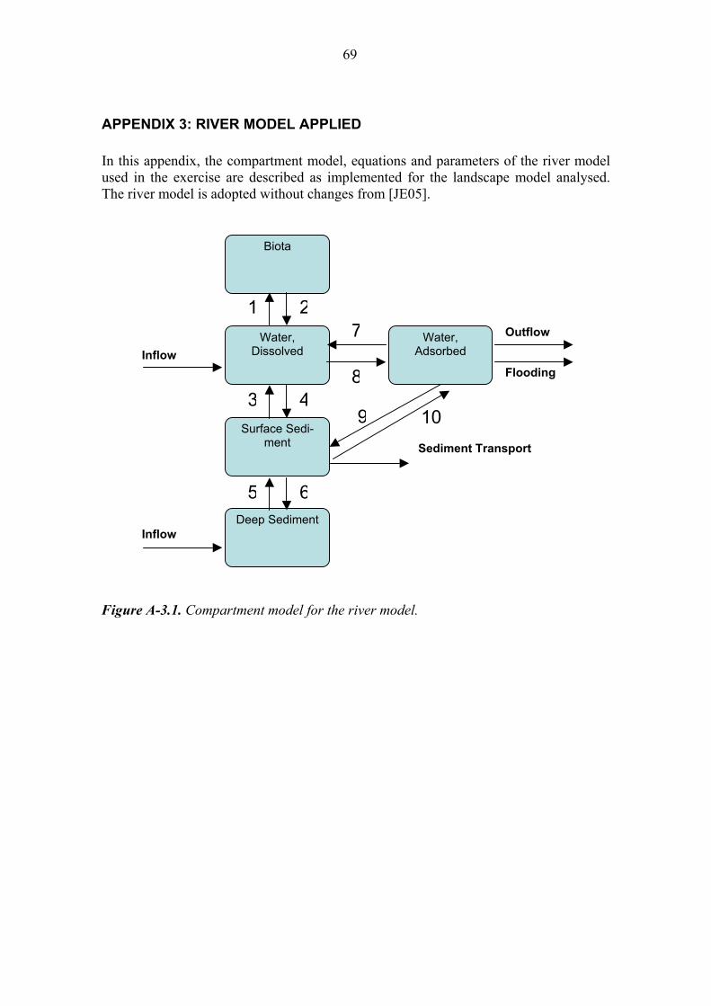
69

APPENDIX 3: RIVER MODEL APPLIED In this appendix, the compartment model, equations and parameters of the river model used in the exercise are described as implemented for the landscape model analysed. The river model is adopted without changes from [JE05].

Figure A-3.1. Compartment model for the river model.

Biota

Inflow

Sediment Transport

Water, Dissolved

Surface Sedi-ment

Deep Sediment

Water, Adsorbed

Flooding Inflow

1 2

3 4

5 6

8

7

9 10

Outflow

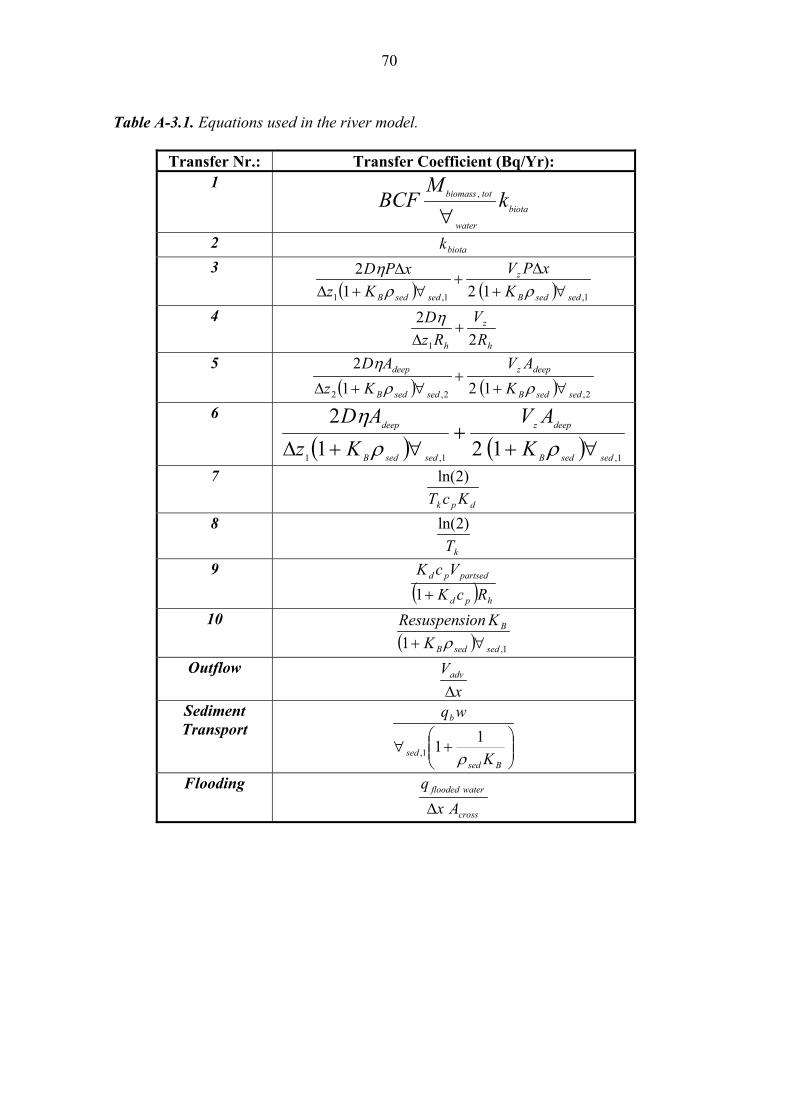
70

Table A-3.1. Equations used in the river model.

Transfer Nr.: Transfer Coefficient (Bq/Yr): 1

biota

water

totbiomass kM

BCF∀

,

2 biotak 3

( ) ( ) 1,1,1 1212

sedsedB

z

sedsedB KxPV

KzxPD

∀+∆

+∀+∆

∆ρρ

η

4

h

z

h RV

RzD

22

1

+∆

η

5 ( ) ( ) 2,2,2 121

2

sedsedB

deepz

sedsedB

deep

KAV

KzAD

∀++

∀+∆ ρρη

6

( ) ( ) 1,1,1 1212

sedsedB

deepz

sedsedB

deep

KAV

KzAD

∀++

∀+∆ ρρη

7

dpk KcT)2ln(

8

kT)2ln(

9 ( ) hpd

partsedpd

RcKVcK

+1

10 ( ) 1,1 sedsedB

B

KKonResuspensi

∀+ ρ

Outflow x

Vadv

∆

Sediment Transport

⎟⎟⎠

⎞⎜⎜⎝

⎛+∀

Bsedsed

b

K

wq

ρ111,

Flooding

cross

waterflooded

Axq∆

71

Table A-3.2. Parameters used in the river model. Some of the parameters in table A-3.2 is used to calculate other parameters, or are calculated from other parameters. For full model-description see [JE05].

Parameter Name Description Kd Distribution coefficient in the stream water KB Distribution coefficient in the sediment Tk Half-time to reach sorption equilibrium BCF Bioconcentration factor qs Specific run-off Aws Watershed area α Cross-sectional angle Sb Slope of the channel ∆x Length of the channel ymax Maximum depth in main channel ρsed Sediment density Vz Advective transport velocity in bed sediment D50, D90 Particle size distribution in the sediment cp Suspended particulate matter in stream water η Sediment porosity D Diffusion coefficient ∆zi Depth of surface and deep sediment Mbiomass Plant biomass n Manning friction coefficient

1,sed∀ Volume of upper sediment

2,sed∀ Volume of deep sediment

water∀ Volume of water

Across Cross-sectional area of water stream Adeep Area of deep sediment equal to area of upper

sediment Vadv Advective velocity Resuspension Resuspension factor Rh Hydraulic radius qflooded water Yearly average of flooded water flowing out of

water stream Vpartsed Sedimentation velocity

72

73

APPENDIX 4: FOREST MODEL APPLIED In this appendix, the compartment model, equations and parameters of the forest model used in the exercise are described as implemented for the landscape model analysed. The forest model from [Avi06] is modified to distribute the input over the full forest area instead of calculating the activity per square meter as originally.

Figure A-4.1. Compartment model for the forest model.

Leaves

Input Outflow

Wood

Litter

Soil

Fauna

Understorey

1

2

3

4

5

6

7

74

Table A-4.1. Equations used in the forest model.

Transfer Nr.: Transfer Coefficient (Bq/Yr): 1

hCRWP W

⋅⋅

ρ

2

hCRLP L

⋅⋅ρ

3

hCRUP U

⋅⋅ρ

4 LToLiTC

5 WToLiTC

6 UToLiTC

Outflow

)( ρθ ⋅+⋅−

KdhETP

Table A-4.2. Parameters used in the forest model. Some of the parameters in table A-4.2 is used to calculate other parameters. For full model-description see [Avi06].

Parameter Name

Description

WP Yearly production of tree wood CRW Concentration ratio of nuclides from soil to tree wood LP Yearly production of tree leaves CRL Concentration ratio of nuclides from soil to leaves UP Yearly production of understorey plants CRU Concentration ratio of nuclides from soil to understorey plants TCLToLi Yearly fractional loss of tree leaves biomass TCWToLi Yearly fractional loss of tree wood biomass TCUToLi Yearly fractional loss of understorey plants biomass ρ Soil bulk density H Thickness of the soil rooting layer P Precipitation rate ET Area normalised evapotranspiration rate θ Volumetric water content in soil Kd Distribution factor in soil

75

APPENDIX 5: Reproducing the results obtained in section 7.

Version of software used: Matlab Ver. 7.1.0.246 (R14) Service Pack 3 Simulink Ver. 6.3 (R14SP3) Pandora Ver 1.0 EIKOS Ver. 2.0

Required files: Apart from the software packages listed above, the following files are required and must be on the Matlab path: TestCase.mdl the model-file ConcEnd.m to extract the solution at t=tfinal Landscape2000AP.m to allow for post-processing within EIKOS (temporary solution only)

Step-by-step guide First the model created in Pandora is opened with EIKOS. At the Matlab prompt, type: > eikos2(Landscape2000AP) Note: the argument (‘Landscape2000AP’) is only necessary to specify for this example case. For other cases, EIKOS is started by simply typing ‘eikos2’ at the Matlab prompt. In the following dialog-window, locate the model file (‘TestCase.mdl’) and open it. In EIKOS we are then given an overview of the model settings, and inputs and outputs (Fig. A-5.1). Depending on what method is to be performed, select the parameters to be included in the analysis either from Table 7.1. (the parameters included in the screen-ing) or from Table 7.2 (the parameters selected for detailed analysis). The selection of inputs/outputs is done by selecting the “Parameters/Outputs” button (Fig. A-5.2). After this, it is necessary to update some of the assigned probability density functions (and min/max values if a method requiring it is to be applied), and this is done by select-ing the “Parameter Settings” option (Fig. A-5.3). The parameter data is then updated using the data listed in table 7.1. The next step is the selection of sensitivity analysis method. The method and method-specific settings are accessed by selecting the “Select SA Method” option (Fig. A-5.4). Once the required method and settings have been applied, the model can be simulated by selecting the “Simulate” option. After the simulation is finished, the results can be viewed graphically by clicking on the “Results” button or choosing any of the plot methods in the “Results” menu. It is also possible to view the results numerically by clicking on any of the four buttons below EIKOS main window (Summary, Input Data, Output Data and Results).

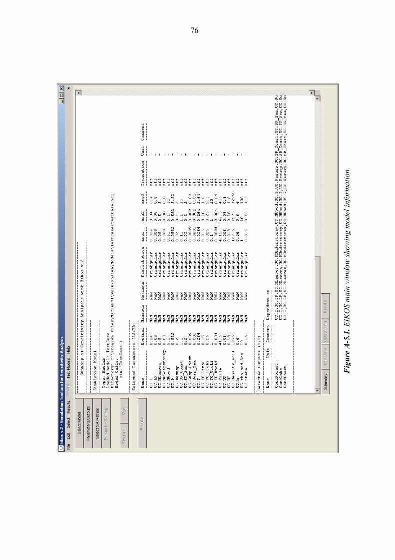
76

Fig

ure

A-5

.1. E

IKO

S m

ain

win

dow

show

ing

mod

el in

form

atio

n.

77

Figure A-5.2. The Parameters/Outputs selection window.

Figure A-5.3. The parameter settings window in EIKOS.

Figure A-5.4. Sensitivity Analysis Method window.