June 2006

Design Guide: UCPRC-DG-2006-01

Sensitivity Analysis of 2002 Design Guide Rigid

Pavement Distress Prediction Models

Authors:

Venkata Kannekanti and John Harvey

This work was completed as part of Partnered Pavement

Research Program Strategic Plan Element 4.1:

“Development of the First Version of a Mechanistic-Empirical Pavement

Rehabilitation, Reconstruction and New Pavement Design Procedure for Rigid and

Flexible Pavements

(pre-Calibration of AASHTO 2002)”

PREPARED FOR:

California Department of Transportation

Division of Research and Innovation Office of

Roadway Research

PREPARED BY:

University of California

Pavement Research Center

Berkeley and Davis

DOCUMENT RETRIEVAL PAGE

Report No: UCPRC-DG-2006-01

Title: Sensitivity Analysis of 2002 Design Guide Rigid Pavement Distress Prediction Models

Authors: Venkata Kannekanti and John Harvey

Prepared for: California Department of Transportation Division of Research and Innovation Office of Roadway Research

FHWA No.: F/CA/DG/2006/48

Date:June 2006,

Final version September 2006

Client Reference Number:

UCPRC-DG-2006-01

Status:

Final

Version No.:3

Abstract: The AASHTO 2002 Design Guide (2002DG) has been calibrated using LTPP sections throughout the nation but with very few sections from the state of California. This created the need to validate the models in 2002DG and recalibrate them if needed so that they may be used for pavement design and rehabilitation in California. In order to validate the design guide, a three-stage process has been identified: bench testing or sensitivity analysis, verification using accelerated pavement testing data, and verification using field data. The study presented in this report includes performing sensitivity analysis of the rigid part of 2002DG. Sensitivity analysis helps to check the reasonableness of the model predictions, to identify problems in the software, and to help understand the level of difficulty involved in obtaining the inputs. The reasonableness of the model predictions is checked by varying key design variables including traffic volume, axle load distribution, climate zone, thickness, shoulder type, joint spacing, load transfer efficiency, PCC strength, base type, and subgrade type. The chosen factorial resulted in approximately 8,500 simulations. The software outputs are transverse cracking, faulting, and IRI. A couple of related sensitivity studies have also been undertaken to study the effect of variables including surface absorptivity and coefficient of thermal expansion, which were not included in the primary sensitivity analysis. Results from all the simulations showed that almost all of the cases produce reasonable values for transverse cracking, faulting, and IRI. The transverse cracking model is sensitive to coefficient of thermal expansion, joint spacing, shoulder type, PCC thickness, and traffic volume. The faulting values are sensitive to dowels, shoulder type, climate zone, PCC thickness and traffic volume. However, there are cases for which model predictions disagree with prevailing knowledge in pavement engineering. This study also revealed some problems associated with the software.

Keywords: Mechanistic-empirical design; Sensitivity analysis; Axle loads; Climate; Pavement distress; Portland cement concrete; Sensitivity analysis; Soil types; Thermal expansion; Thickness; Traffic volume

Proposals for implementation: It is proposed to develop sample design catalogs for rigid pavements based on the DG2002 software coupled with Caltrans experience. Final designs should not be based exclusively on performance predictions from the current version of the software.

Related documents: Transportation Research Board Annual Meeting 2006 Paper #06-1893 (accepted for publication at the Transportation Research Records Journal)

Signatures:

Venkata Kannekanti

First Author

Erwin Kohler Technical Review

C. Scheffy, original. D. Spinner, revised material

Editor

John Harvey Principal

Investigator

Michael Samadian Caltrans Contract

Manager

UCPRC-DG-2006-01

iii

DISCLAIMER The contents of this report reflect the views of the authors who are responsible for the facts and accuracy of the

data presented herein. The contents do not necessarily reflect the official views or policies of the State of

California or the Federal Highway Administration. This report does not constitute a standard, specification, or

regulation.

UCPRC-DG-2006-01

iv

TABLE OF CONTENTS

List of Figures.....................................................................................................................................................vii List of Tables ....................................................................................................................................................... ix Executive Summary.............................................................................................................................................. x 1. Introduction....................................................................................................................................................... 1

1.1 NCHRP 1-37a Project Background......................................................................................................... 1 1.2 Objectives of the Study ........................................................................................................................... 2 1.3 Scope of the Report ................................................................................................................................. 2

2. Experiment Design ........................................................................................................................................... 3 2.1 Traffic Inputs........................................................................................................................................... 4

2.1.1 Two-way Annual Average Daily Truck Traffic (AADTT)............................................................. 4 2.1.2 Traffic Volume Adjustment Factors ............................................................................................... 4 2.1.3 Axle Load Distribution Factors....................................................................................................... 5 2.1.4 General Traffic Inputs..................................................................................................................... 5

2.2 Climate .................................................................................................................................................... 5 2.3 Pavement Design Features ...................................................................................................................... 7 2.4 Drainage and Surface Properties ............................................................................................................. 7 2.5 Pavement Structure ................................................................................................................................. 7 2.6 Layer Properties ...................................................................................................................................... 8

2.6.1 PCC Slab......................................................................................................................................... 8 2.6.2 Asphalt Concrete Base .................................................................................................................... 8 2.6.3 Cement Treated Base ...................................................................................................................... 9 2.6.4 Aggregate Subbase.......................................................................................................................... 9 2.6.5 Subgrade ......................................................................................................................................... 9

2.7 Difficulty in Obtaining Sufficient Input Data ......................................................................................... 9 2.7.1 Traffic ............................................................................................................................................. 9 2.7.2 Climate.......................................................................................................................................... 10 2.7.3 Pavement Design Features ............................................................................................................ 10 2.7.4 Drainage and Surface Properties................................................................................................... 10 2.7.5 PCC Layer Properties.................................................................................................................... 10 2.7.6 Cement Treated Bases................................................................................................................... 11 2.7.7 Asphalt Concrete Bases ................................................................................................................ 11 2.7.8 Unbound Materials (Aggregate Base and Subgrade).................................................................... 11

3. Results and Analysis....................................................................................................................................... 12 3.1 Effect of Variables on Transverse Cracking ......................................................................................... 13

UCPRC-DG-2006-01

v

3.1.1 Effect of Shoulder Type................................................................................................................ 13 3.1.2 Effect of Joint Spacing on Cracking ............................................................................................. 14 3.1.3 Effect of Climate on Cracking ...................................................................................................... 15 3.1.4 Effect of Traffic Volume............................................................................................................... 16 3.1.5 Effect of Subgrade Type ............................................................................................................... 16 3.1.6 Effect of Slab Thickness ............................................................................................................... 18 3.1.7 Effect of Base Type....................................................................................................................... 18 3.1.8 Effect of Load Spectra .................................................................................................................. 18 3.1.9 Effect of Dowels ........................................................................................................................... 20 3.1.10 Effect of PCC Flexural Strength ................................................................................................... 20 3.1.11 Summary ....................................................................................................................................... 20

3.2 Effect of Variables on Faulting ............................................................................................................. 23 3.3 Effect of Variables on IRI ..................................................................................................................... 28 3.4 Comparison of IRI Models from 2002DG and Ripper Study ............................................................... 36 3.5 Effect of Coefficient of Thermal Expansion on Transverse Cracking, Faulting, and IRI..................... 38 3.6 Summary of Sensitivity Analysis Results ............................................................................................. 40

4. Anomalies in the Predictions .......................................................................................................................... 43 4.1 Shortwave Surface Absorptivity ........................................................................................................... 43 4.2 Cases for which Thinner Pavement Sections Perform Better Than Thicker Sections........................... 47

4.2.1 Cases for which Structures with 7-in. Slabs Perform Better Than Those with 8-in. Slabs........... 47 4.2.2 Cases for which Structures with 8-in. Slabs Perform Better Than Those with 9-in. Slabs........... 47 4.2.3 Cases for which Structures with 9-in. Slabs Perform Better Than Those with 10-in. Slabs ......... 47 4.2.4 Cases for which Structures with 10-in. Slabs Perform Better Than Those with 12-in. Slabs ....... 48

4.3 Cases for which Structures with Asphalt Shoulders Perform Better Than Structures with Tied

Shoulders .......................................................................................................................................... 48 4.4 Cases for which Structures with Asphalt Shoulder Perform Better Than Structures with Widened

Truck Lanes ...................................................................................................................................... 48 4.5 Cases for which Tied Shoulder Structures Perform Better Than Structures with Wide Truck Lanes... 49 4.6 Subgrade................................................................................................................................................ 49 4.7 High K-value of Subgrade..................................................................................................................... 56

5. Limitations and Bugs in the Software............................................................................................................. 57 5.1 Inability to Reproduce Results .............................................................................................................. 57 5.2 Base Properties...................................................................................................................................... 57 5.3 Aggregate Type..................................................................................................................................... 59 5.4 Climate Data.......................................................................................................................................... 59 5.5 Running the Software in Batch Mode ................................................................................................... 60

UCPRC-DG-2006-01

vi

5.6 Spalling Not Included in Output ........................................................................................................... 60 5.7 Other Problems...................................................................................................................................... 61

6. Conclusions..................................................................................................................................................... 64 7. References....................................................................................................................................................... 66 8. Appendix A: Screen Shots from the Software ................................................................................................ 67

UCPRC-DG-2006-01

vii

LIST OF FIGURES

Figure 1. Axle load spectra from WIM located in a rural area (Site No. 2, Redding, SHA I-5)........................... 6 Figure 2. Axle load spectra from a WIM located in an urban area (Site No. 39, Redlands, SBD SR-30)............ 6 Figure 3. Pavement structure used for the sensitivity study.................................................................................. 8 Figure 4. Key to understanding the plots. ........................................................................................................... 13 Figure 5. Effect of shoulder type on transverse cracking.................................................................................... 14 Figure 6. Effect of joint spacing on transverse cracking..................................................................................... 15 Figure 7. Effect of climate region on transverse cracking. ................................................................................. 16 Figure 8. Effect of traffic volume on transverse cracking. ................................................................................. 17 Figure 9. Effect of subgrade type on transverse cracking. .................................................................................. 17 Figure 10. Effect of PCC thickness on transverse cracking................................................................................ 19 Figure 11. Effect of base type on transverse cracking. ....................................................................................... 19 Figure 12. Effect of load spectra on transverse cracking. ................................................................................... 20 Figure 13. Effect of PCC flexural strength on transverse cracking. ................................................................... 21 Figure 14. Relative effect of all variables on transverse cracking. ..................................................................... 22 Figure 15. Effect of dowels on faulting. ............................................................................................................. 23 Figure 16. Effect of climate region on faulting................................................................................................... 24 Figure 17. Effect of PCC thickness on faulting .................................................................................................. 24 Figure 18. Effect of traffic index (TI) on faulting............................................................................................... 25 Figure 19. Effect of shoulder type on faulting. ................................................................................................... 25 Figure 20. Effect of joint spacing on faulting. .................................................................................................... 26 Figure 21. Effect of base type on faulting........................................................................................................... 26 Figure 22. Effect of subgrade on faulting. .......................................................................................................... 27 Figure 23. Effect of load spectra on faulting. ..................................................................................................... 27 Figure 24. Effect of PCC flexural strength on faulting....................................................................................... 28 Figure 25. Relative effect of all variables on faulting......................................................................................... 29 Figure 26. Effect of PCC thickness on IRI. ........................................................................................................ 31 Figure 27. Effect of shoulder type on IRI. .......................................................................................................... 32 Figure 28. Effect of traffic index (TI) on IRI...................................................................................................... 32 Figure 29. Effect of dowels on IRI. .................................................................................................................... 33 Figure 30. Effect of joint spacing on IRI. ........................................................................................................... 33 Figure 31. Effect of load spectra on IRI. ............................................................................................................ 34 Figure 32. Effect of base type on IRI.................................................................................................................. 34 Figure 33. Effect of subgrade type on IRI. ......................................................................................................... 35 Figure 34. Effect of PCC flexural strength on IRI. ............................................................................................. 35

UCPRC-DG-2006-01

viii

Figure 35. Effect of climate region on IRI.......................................................................................................... 36 Figure 36. Relative effect of all variables on IRI................................................................................................ 37 Figure 37. Comparison of IRI models from 2002DG and Ripper study............................................................. 39 Figure 38. Effect of COTE on transverse cracking............................................................................................. 40 Figure 39. Effect of COTE on faulting. .............................................................................................................. 41 Figure 40. Effect of surface absorptivity on transverse cracking, an example. .................................................. 44 Figure 41. Effect of surface absorptivity on transverse cracking........................................................................ 45 Figure 42. Effect of surface absorptivity on faulting. ......................................................................................... 45 Figure 43. Effect of surface absorptivity on transverse cracking compared to other variables. ......................... 46 Figure 44. Effect of surface absorptivity on faulting compared to other variables............................................. 46 Figure 45. Pavement structure used to study the effect of soil type.................................................................... 50 Figure 46. Faulting for different subgrade types, undoweled pavements. .......................................................... 52 Figure 47. Faulting for different subgrade types, doweled pavements. .............................................................. 52 Figure 48. Cracking for different subgrade types, both doweled and undoweled pavements............................. 53 Figure 49. Effect of subgrade on DE for undoweled pavements according to 2002DG. ....................................... 55 Figure 45. Base Properties input screen shots..................................................................................................... 58 Figure 46. Structure window screen shot............................................................................................................ 59 Figure 47. Error message when Ukiah climate file was used. ............................................................................ 60 Figure 48. Batch file window.............................................................................................................................. 61 Figure 49. Error message. ................................................................................................................................... 61 Figure 50. Debug mode. ..................................................................................................................................... 62 Figure 51. Screen shot showing that inputs could not be entered. ...................................................................... 63 Figure 52. Error message when PCC thickness is chosen as 10 in. .................................................................... 63 Figure A1. General Traffic Inputs (Number Axles/Truck tab) ........................................................................... 67 Figure A2. General Traffic Inputs (Axle Configuration tab) .............................................................................. 68 Figure A3. General Traffic Inputs (Wheelbase tab)............................................................................................ 69 Figure A4. JPCP Design Features....................................................................................................................... 70 Figure A5. PCC Material Properties (Thermal properties tab). .......................................................................... 71 Figure A6. PCC Material Properties (Mix properties tab). ................................................................................. 72 Figure A7. PCC Material Properties (Strength tab). ........................................................................................... 73 Figure A8. Asphalt Material Properties (Asphalt Mix tab)................................................................................. 74 Figure A9. Asphalt Material Properties (Asphalt Binder tab). ........................................................................... 75 Figure A10. Asphalt Material Properties (Asphalt General tab)......................................................................... 76 Figure A11. Cement/Lime Stabilized Material (Cement Stabilized option)....................................................... 77 Figure A12. Unbound Layer #3 (Strength Properties tab, A-1-a option). .......................................................... 78 Figure A13. Unbound Layer #3 (ICM tab). ........................................................................................................ 79

UCPRC-DG-2006-01

ix

Figure A14. Unbound Layer #4 (Strength Properties tab, CH material option). ................................................ 80 Figure A15. Unbound Layer #4 (Strength Properties tab, SP material option) .................................................. 81 Figure A16. Unbound Layer #4 (ICM tab, CH material option). ....................................................................... 82 Figure A17. Unbound Layer #4 (ICM tab, SP material option). ........................................................................ 83

LIST OF TABLES

Table 1 Variables and Factor Levels Used for Sensitivity Analysis of 1-37a...................................................... 3 Table 2 Two-way AADTT at Both WIM Stations for All Three TI Values* ...................................................... 4 Table 3 Annual Average Weather Data for the Three Climate Regions Used in the Study................................. 7 Table 4 Experiment Design to for Study of the Effect of the Coefficient of Thermal Expansion (COTE) ....... 39 Table 5 Mean Results of Sensitivity Analysis for Each Variable and Factor Level .......................................... 42 Table 6 Experiment Design for Study of the Effect of Surface Absorptivity .................................................... 43 Table 7 Key Inputs Used to Study the Effect of Soil Type ................................................................................ 50 Table 8 Performance of Structures with Different Soil Types and without Dowels .......................................... 51 Table 9 Performance of Structures with Different Soil Types and with Dowels ............................................... 51 Table 10 DE Estimation Based on EverFE Runs......................................................................................... 55 Table 11 Default P200 Values Used in the Study.......................................................................................... 55 Table 12 Effect of P200 on Faulting, Cracking, and IRI for Undoweled Pavements .................................. 56

UCPRC-DG-2006-01

x

EXECUTIVE SUMMARY

The AASHTO 2002 Design Guide (2002DG) has been calibrated using Long Term Pavement Performance

(LTPP) sections scattered throughout the nation but with very few sections from the state of California. This

created the need to validate the models in 2002DG and recalibrate them if needed so that they may be used for

pavement design and rehabilitation in California. In order to validate the design guide, a three-stage process

has been identified: bench testing or sensitivity analysis, verification using accelerated pavement testing data,

and verification using field data. The study presented in this report includes performing sensitivity analysis of

the rigid part of 2002DG.

Sensitivity analysis helps to check the reasonableness of the model predictions, to identify problems in

the software and to help understand the level of difficulty involved in obtaining the inputs. The reasonableness

of the model predictions is checked by varying key design variables including traffic volume, axle load

distribution, climate zone, thickness, shoulder type, joint spacing, load transfer efficiency, PCC strength, base

type, and subgrade type. The chosen factorial resulted in approximately 8,500 simulations. The software

outputs are transverse cracking, faulting, and IRI. A couple of related sensitivity studies have also been

undertaken to study the effect of variables including surface absorptivity and coefficient of thermal expansion,

which were not included in the primary sensitivity analysis.

Results from all the simulations showed that almost all of the cases produce reasonable values for

transverse cracking, faulting, and IRI. The transverse cracking model is sensitive to coefficient of thermal

expansion, joint spacing, shoulder type, PCC thickness, and traffic volume. The faulting values are sensitive to

dowels, shoulder type, climate zone, PCC thickness and traffic volume. However, there are cases for which

model predictions disagree with prevailing knowledge in pavement engineering. This study also revealed some

problems associated with the software.

1

1. INTRODUCTION

The AASHO (American Association of State Highway Officials) road test was performed in 1958. It

has been over 40 years since empirical-based pavement design procedures were developed based on the

AASHO road test. Few changes were made to these procedures over the years despite the many limitations of

the test. Some of the limitations of the AASHO road test are:

• One climate region

• Limited traffic

• One vehicle type

• One subgrade type

Because of the limitations of the empirical procedures based on the road test, the AASHTO (American

Association of State Highway and Transportation Officials) Joint Task Force on Pavements (JTFP) took the

initiative to develop a new pavement design guide. The JTFP proposed that the new design guide should be

based on well-established mechanistic-empirical models and utilize more comprehensive data sets, such as

Long Term Pavement Performance (LTPP) data. The JTFP’s initiative resulted in NCHRP Project 1-37a.

1.1 NCHRP 1-37a Project Background

The objective of NCHRP 1-37a is to develop a pavement design tool based on mechanistic-empirical

principles. The resulting pavement design tool, called the 2002 Design Guide (2002DG), is intended to be

user-friendly software for analysis and design of new, reconstructed, and rehabilitated flexible, rigid, and

composite pavements. The 2002 Design Guide is a result of coordinated effort of NCHRP Project Panel C1-37

and AASHTO JTFP. The models in the design guide were calibrated using data from LTPP sections from all

over the nation. However, very few sections from California were used for calibration of the models in

2002DG.

AASHTO recommends that each state validate and, if necessary, recalibrate the models using the

climate, traffic, and materials data more representative of each state. The validation process adopted in

California consists of three steps:

• Bench testing or sensitivity analysis,

• Validation using accelerated pavement testing data, and

• Validation using field data.

The models will be recalibrated using California field data if validation results show serious

discrepancies between the observed distresses and the distresses predicted by the models. The study presented

in this report concentrates only on the sensitivity analysis of the software. The following section explains the

objectives of the sensitivity analysis.

2

1.2 Objectives of the Study

The objectives of the study presented herein are:

1. Evaluate the reasonableness of rigid pavement design models in 2002DG for California traffic and

climate conditions.

2. Estimate the level of difficulty in using 2002DG design procedures for designing new rigid

pavements in California.

3. Identify any problems or bugs evident in the software.

The reasonableness of the model predictions are checked by varying key design variables like traffic

volume, axle load distribution, climate zone, thickness, shoulder type, joint spacing, load transfer efficiency,

PCC strength, base type, and subgrade type. The software was run for all combinations of these key variables

and the results from cases were compared.

1.3 Scope of the Report

The experiment design used for sensitivity analysis is explained in Chapter 2. Chapter 2 also discusses

the inputs used to run the sensitivity analysis, the source of these inputs, and the level of difficulty in obtaining

the inputs to run the software.

The results of sensitivity analysis are discussed in Chapter 3. Various plots summarizing the effects of

different variables on transverse cracking, faulting and IRI are presented.

Chapter 4 describes cases in the sensitivity analysis where results disagree with the prevailing

knowledge in pavement engineering.

Chapter 5 discusses the problems and bugs associated with the software.

Conclusions from the sensitivity analysis are presented in Chapter 6.

3

2. EXPERIMENT DESIGN

Some important variables that affect the pavement design software were selected and the software was

run for several factor levels for the selected variables. The variables selected for the sensitivity study and the

factor levels used are shown in Table 1. To the extent possible, the variables and factor levels were chosen to

represent the practices adopted by the California Department of Transportation (Caltrans).

Table 1 Variables and Factor Levels Used for Sensitivity Analysis of 1-37a Variable Factor Levels

1 Axle Load Spectra (2) Urban Rural

2 Traffic Volume (3) TI: 12 13 16

3 Climate Region (3) South Coast (Los Angeles) Valley (Sacramento) Mountain (Reno)1

4 PCC Thickness (5)

7 in. 8 in. 9 in. 10 in. 12 in.

5 Base Type (2) Asphalt Concrete Base Cement Treated Base

6 Subgrade Type (2) High Plasticity Clay (CH) Poorly graded sand (SP)

7 Dowels (2) Dowels No Dowels

8 Shoulder Type (3) Asphalt Shoulders Tied Shoulders Widened Truck Lane

9 Joint Spacing (2) 15 ft. 19 ft.

10 Strength 2 (2) 626 psi 700 psi

Total Number of Cases: 8,640 1 Reno though in Nevada, has climate similar to high desert and mountain climate zones of California and has good climate data and so is used in this study. 2 28-day PCC flexural strength. All cases were run with a reliability level of 50% and a design life of 30 years. A detailed discussion

of the inputs and the sources of inputs are presented in the next section. The software allows a hierarchical

approach to enter the inputs at three levels. Level 1 inputs yield accurate results, but the inputs require lot of

lab and field testing and consume more time and resources. Level 2 inputs are obtained from agency databases

or estimated through correlations. Level 3 inputs are default values or typical averages for the project location

and materials used.

4

2.1 Traffic Inputs

Most of the traffic inputs are derived from Caltrans weigh-in-motion (WIM) data. WIM data at two

locations (Urban and Rural) with three volumes of traffic, in the form of Traffic Index (TI) have been used for

this study. Urban locations have more Class 5 trucks (short trailers) than Class 9 trucks (long trailers) and rural

locations have more Class 9 trucks.

The urban location used for this analysis is WIM station 02 located on I-5 at Redding. The rural

location is represented by WIM station 39 on SR-30 at Redlands. The three traffic volumes (TI values of 12,

13, and 16) correspond to approximately 11 million, 22 million, and 126 million ESALs, respectively.

2.1.1 Two-way Annual Average Daily Truck Traffic (AADTT)

The AADTT corresponding to the two locations and traffic spectra are given in Table 2. AADTT

information for each TI is estimated using WIM data. TI is first converted into axles. AADTT is calculated

based on the average number of axles per truck for that site.

Table 2 Two-way AADTT at Both WIM Stations for All Three TI Values* Spectra\TI 12 13 16

Rural (WIM 02) 990 1968 11256

Urban (WIM 39) 1766 3462 19820

*Erratum: Due to a misinterpretation, AADTTs in the table actually represent TIs of 11.4, 12.4, and 15.3 for rural spectra and TIs of 11.6, 12.6, and 15.5 for urban spectra. This correction has no effect on the observations/conclusions of this report.

2.1.2 Traffic Volume Adjustment Factors

Traffic volume adjustment factors are used to determine AADTT within each hour of the day for each

month and for each truck class. This determination requires the following:

• Hourly truck distribution factors

• Vehicle class distribution factors

• Monthly adjustment factors

Each of these factors is obtained from the WIM data. In addition to traffic volume adjustment factors,

the expected growth rate must be entered for the AADTT. In this study, growth rate is assumed to be zero

because all the truck traffic is uniformly distributed for the entire design life. This assumption has little effect

on the results because Miner’s law, which assumes a linear damage rate with traffic repetitions, is used for

damage accumulation in the distress prediction models. The only sensitivity of the results would be due to

PCC strength gain effects.

5

2.1.3 Axle Load Distribution Factors

The normalized axle load distributions used in this study are determined from the WIM data. The axle

load distribution is entered for single axles, tandem axles, tridem axles, and quad axles. Urban and rural

locations have significantly different axle load distributions. The axle load distributions for both the locations

chosen are shown in Figures 1 and 2. The 2002 Design Guide requires the axle load distribution factors for

each month and for each class of vehicle, however, Figures 1 and 2 give the axle load distribution frequency

for all truck classes combined and for all months. Nevertheless, the plots show the basic difference in axle load

distribution at the two locations. Very few trucks with quad axles operate in California, so the axle load

distribution factors for quad axles are assumed to be zero.

2.1.4 General Traffic Inputs

This category of inputs include information like mean wheel location, traffic wander standard

deviation, design lane width, wheel base information, tire dimensions, and tire inflation pressures. Default

values have been used for all of the general traffic inputs. The screen shots of the inputs used are shown in

Appendix A. Other information in this category includes the number of axle types per truck class and axle

configuration, which were obtained from WIM data and are also presented in Appendix A.

2.2 Climate

All of the necessary climate information at any given location can be generated by simply selecting

the weather station near the location of pavement construction. The three climate regions used for the

sensitivity analysis are:

• South Coast (Los Angeles)

• Valley (Sacramento)

• Mountain/High Desert (Reno)

Table 3 shows the differences in temperatures and precipitation for the three climate regions. These

values are obtained from Climate Database for Integrated Model (CDIM) software version 1.0, which is based

on daily and hourly weather data in the western half of the United States. The Mountain/High Desert climate

zone will be addressed as mountain climate zone for the rest of the report.

One other climate input required for analysis is the depth of the water table. A default value of 30 feet

is assumed for all the three climate regions.

6

0

0.02

0.04

0.06

0.08

0.1

0.12

0.14

0.16

0.18

0.2

0 5 10 15 20 25 30 35 40 45

Load Range

Axl

e Lo

ad F

requ

ency

SingleTandemTridem

Figure 1. Axle load spectra from WIM located in a rural area (Site No. 2, Redding, SHA I-5).

0

0.02

0.04

0.06

0.08

0.1

0.12

0.14

0.16

0.18

0.2

0 5 10 15 20 25 30 35 40 45

Load Range

Axl

e Lo

ad F

requ

ency

SingleTandemTridem

Figure 2. Axle load spectra from a WIM located in an urban area (Site No. 39, Redlands, SBD SR-30).

7

Table 3 Annual Average Weather Data for the Three Climate Regions Used in the Study Weather Data\Climate Region Los Angeles Sacramento Reno Lowest Air Temperature (ºC) 3 -3.3 -17.4 Highest Air Temperature (ºC) 36.5 41.4 38.4 Freezing Index (ºC–Days) 0 0 119 Number of Freeze-Thaw Cycles 0 3 116 Total Yearly Precipitation (mm) 325 446 193 Total Yearly Snowfall (mm) 0 1 627

2.3 Pavement Design Features

Pavement design features include joint spacing, shoulder type, load transfer efficiency, and PCC-base

interface. Joint spacing of 15 and 19 feet were used for this study. Three different shoulder types have been

considered: asphalt shoulders, widened truck lane, and tied shoulders. A default load transfer of 40% between

the slab and the shoulder is assumed for tied shoulders. Wide truck lanes are 14 feet wide, two feet wider than

the normal width. Two cases of load transfer efficiencies are considered, doweled and undoweled. For doweled

pavements, the diameter of dowels is 1.5 in. and dowel spacing is 12 in. The permanent curl/warp effective

temperature difference is assumed to be –10ºF (with the top of the slab cooler than the bottom of the slab). The

joint sealant type is assumed to be silicone. It is assumed that there is no bonding between the base and the

PCC slab. Erodibility Index of the base is assumed to be 3, meaning that the base material is erosion resistant.

A screen shot of the JPCP Design Features input window is shown in Appendix A.

2.4 Drainage and Surface Properties

This category of inputs includes surface shortwave absorptivity, infiltration, drainage path length, and

pavement cross slope. The default value used in the software for surface shortwave absorptivity is 0.85 and this

value is used for calibrating the models in the software. However, in this study surface absorptivity is assumed

to be 0.65, based on a study conducted by Lawrence Berkeley National Laboratory, which indicated that new

rigid pavements have surface absorptivity of 0.65.(1) Default values are used for drainage parameters. Values

assumed for infiltration, drainage path length, and pavement cross slopes are 10%, 12 ft., and 2% respectively.

2.5 Pavement Structure

The assumed pavement structure is a PCC slab of one of several thicknesses (7, 8, 9, 10, or 12 in.), 6

inches of cement treated base or asphalt concrete base, 6 inches of aggregate subbase, and CH or SP subgrade.

Figure 3 shows the pavement structure used for the study.

8

Figure 3. Pavement structure used for the sensitivity study.

2.6 Layer Properties

2.6.1 PCC Slab

The unit weight of PCC used is 150 pcf. Default values were used for thermal properties. Type II

cement is used with a cement content of 657 lb./cu. yd. and a water-to-cement ratio of 0.42. Default values

were used for shrinkage parameters. Values for 28-day flexural strength were 626 psi and 700 psi. Flexural

strength of 626 psi corresponds to the Ludlow mix used for the PPRC Maturity Project (2) and meets the

Caltrans standard specification.

The second factor level for strength is 700 psi, about 10% higher than the standard strength of 626 psi.

The same mix design parameters were used for both flexural strength cases. Screen shots of the PCC thermal,

mix, and strength input windows are shown in Appendix A.

2.6.2 Asphalt Concrete Base

Level 3 inputs are used for the asphalt concrete base. Conventional viscosity grade of AC 10 is used

for binder properties. The base is assumed to have 8% air-void content. Screen shots of asphalt mix, binder,

and general properties (including aggregate gradation) input windows are shown in Appendix A.

9

2.6.3 Cement Treated Base

The elastic modulus is assumed to be 2,000,000 psi. Default values are used for thermal properties of

the cement treated base. Appendix A includes a screen shot of the “Cement/Lime Stabilized Material” input

window.

2.6.4 Aggregate Subbase

Level 3 inputs are used for the subbase properties. Modulus of 40,000 psi is assumed. Screen shots of

subbase properties input windows are shown in Appendix A.

2.6.5 Subgrade

Two types of subgrades are assumed in this study: high plasticity clay and poorly graded sand with

CH and SP as corresponding USC soil classifications. Level 3 inputs are used for the subgrades. Default

moduli of 8,000 psi and 28,000 psi are assumed for CH and SP respectively. Screen shots of subgrade

properties input windows are shown in Appendix A.

2.7 Difficulty in Obtaining Sufficient Input Data

The most time-consuming and difficult part in designing a pavement using the mechanistic-empirical

approach is to get the required inputs. The 2002DG is no exception. To a great extent, the ability to implement

this software depends on the cost of getting these inputs. The designer can always fall back on Level 3 inputs

(default values) for almost all of the variables in the software, but will have to compromise on the accuracy of

the performance predictions. Level 3 inputs are recommended only for projects with minimal consequences of

early failure. In this section, the inputs that are difficult to estimate, forcing the designer to adopt Level 3

inputs, are addressed.

2.7.1 Traffic

Traffic inputs are the easiest to obtain, provided WIM data near the project location is available. In the

absence of WIM data, Level 3 default values need to be used or regional values can be used by deriving them

from WIM stations present in the vicinity.

However, some inputs cannot be obtained from the WIM data so default values have been used for

this study. Inputs that fall in this category are

• Traffic wander standard deviation,

• Mean wheel location from the lane markings, and

• Dual tire spacing.

The default values that were used in this analysis can be found in Appendix A.

10

2.7.2 Climate

Climate data can be obtained from the weather station present in the vicinity of the pavement

construction location. In the absence of a weather station, a virtual weather station can be used by interpolating

data from weather stations near the project site. Another climate input is the depth of water table, which can be

very difficult to estimate.

2.7.3 Pavement Design Features

Erodibility Index of the base and the number of months for loss of bond between the base and PCC

slab are very subjective and there is no method to estimate these values.

2.7.4 Drainage and Surface Properties

Surface absorptivity is generally not measured by agencies but it turns out that surface absorptivity is

the key variable in predicting transverse cracking. This will be discussed later in this report. Infiltration

potential of the pavement over its design life is again very subjective.

2.7.5 PCC Layer Properties

Thermal properties of the PCC layer (coefficient of thermal expansion, thermal conductivity, and heat

capacity) need to be estimated by laboratory tests according to standard methods. The coefficient of thermal

expansion is supposed to be determined using the test method AASHTO TP60. Thermal conductivity and heat

capacity are supposed to be determined by using test methods ASTM E 1952 and ASTM D 2766, respectively.

Currently, Caltrans is not equipped with the instruments required to perform these tests nor does it have

personnel trained to do such tests.

The other input parameters that are difficult to estimate are:

• PCC Zero stress temperature (option of computing internally by the software)

• Ultimate shrinkage at 40% relative humidity (AASHTO T 160 protocol)

• Reversible shrinkage as percent of ultimate shrinkage (option of computing internally by the

software)

• Time in days to develop 50% of ultimate shrinkage (AASHTO T 160 protocol)

The Level 1 and Level 2 strength properties require the user to enter values for 7-day, 14-day, 28-day,

90-day Young’s modulus, modulus of rupture, or compressive strength. These values must be pulled out of a

database based on the mix designs.

11

2.7.6 Cement Treated Bases

Thermal conductivity and heat capacity should be determined by using test methods ASTM E 1952

and ASTM D 2766, respectively. Caltrans is currently not equipped to perform these tests.

2.7.7 Asphalt Concrete Bases

Level 1 asphalt mix properties require triaxial frequency sweep test data at temperatures 10º, 40º, 70º,

100º, and 130ºF. It is very difficult to get any values at a temperature of 130ºF using the triaxial test.

2.7.8 Unbound Materials (Aggregate Base and Subgrade)

A representative value of resilient modulus or soil indices like CBR, R-value, Layer coefficient, or

Penetration (from Dynamic Cone Penetrometer) needs to be entered. Resilient modulus needs to be calculated

according to test methods from NCHRP 1-28, Harmonized Test Methods for Laboratory Determination of

Resilient Modulus for Flexible Pavement Design or AASHTO T 307, Determining the Resilient Modulus of

Soil and Aggregate Materials. The Enhanced Integrated Climate Model (EICM) is used to modify the

representative modulus of rupture (Mr) for the seasonal effects of climate changes. The inputs required by

EICM include gradation and Plasticity Index, which should be calculated using AASHTO T 99. In order to

estimate the moisture profile through the pavement structure, EICM requires the following inputs, which can

either be entered by the user or calculated internally by the 2002DG software:

• Maximum dry unit weight

• Specific gravity of solids

• Saturated hydraulic conductivity

• Optimum gravimetric content

Estimating these parameters requires additional testing of the sample and is difficult. The user also has

the option to enter the soil water characteristic curve parameters, which requires additional testing.

12

3. RESULTS AND ANALYSIS

All the variables and factor levels in Table 1 were run using the software and the results loaded into a

database. The software was run in batch mode for which the cracking and the faulting models need to be run

separately. Note that the batch mode option in the Tools menu of the software was not used here. Instead,

another way suggested by one of the developers of the software was used to run cracking and faulting models

separately in batch mode. Making this a standard feature in the software would facilitate large scale analysis.

Faulting and cracking values were obtained for all the cases for 50% reliability and after 30 years of

life. After getting the faulting and cracking values, empirical equations mentioned in the Design Guide’s user

manual are used to estimate spalling and IRI .

Sensitivity analysis was begun before an official version of the software was available from the

FHWA, so all cases were run using a draft version of the software. After receiving the official version of the

software some cases were re-run. Results from the latest software matched those from the pre-approved

version, indicating no major changes had been made.

The results from the cases run enabled the isolation of the effect of various variables on faulting,

transverse cracking, and IRI. The effect of all the variables in the sensitivity study on faulting, transverse

cracking, and IRI are discussed in the following sections.

In the plots presented in the following sections, the lowest horizontal line is the lowest value found in

the data set. The second horizontal line is the 25th percentile value, third line gives the median or the 50th

percentile value, fourth horizontal line gives the 75th percentile value and the top most horizontal line gives the

maximum value present in the data set. A key to understanding the plots is shown in Figure 4.

13

Key

highest value present in data set

75th percentile value

50th percentile (median) value

25th percentile value

lowest value present in data set

Figure 4. Key to understanding the plots.

3.1 Effect of Variables on Transverse Cracking

The transverse cracking model in 2002DG predicts transverse cracking as percent of slabs cracked.

The effects of different variables in the sensitivity study on transverse cracking, as predicted by the 2002DG,

are presented in the following sections.

3.1.1 Effect of Shoulder Type

Pavement structures with a widened truck lane have been shown to perform better than those with tied

shoulders or with asphalt shoulders.(3) Widened truck lanes reduce cracking considerably as shown in

Figure 5.

The plot shows that cases exist for which structures with widened truck lanes have 100% cracking.

These cases are structures with very high traffic loading in valley or mountain regions having joint spacing of

19 ft. and 7-in. slab thickness. The median values for the three shoulder types (shown as horizontal line with a

dot) indicate that on average, structures with widened truck lane or tied shoulders perform better than

structures with asphalt shoulders.

14

AsphaltShoulder

Tied WidenedLane

Shoulder Type

0

20

40

60

80

100

% S

labs

Cra

cked

Figure 5. Effect of shoulder type on transverse cracking.

3.1.2 Effect of Joint Spacing on Cracking

Joint spacing is the key variable that controls transverse cracking. The results from the sensitivity

analysis show a dramatic difference in cracking between structures with joint spacing of 19 ft. versus 15 ft.

Joint spacing of 19 ft. is very detrimental to the pavement. Figure 6 summarizes the effect of joint spacing. The

plot indicates that only 25% of the structures with 15-ft. joint spacing have more than 18% cracking whereas

75% of the structures with 19-ft. joint spacing have more than 20% cracking. The plot shows that there are

some cases with 15-ft. joint spacing that have a very high degree of cracking. These cases correspond to

structures subjected to heavy traffic loading, with asphalt shoulders and thin slabs. The cases having 19-ft.

joint spacing with low cracking are structures subjected to low traffic located in the south coast (Los Angeles)

climate zone.

15

15 19

Joint Spacing (ft.)

0

20

40

60

80

100

% S

labs

Cra

cked

Figure 6. Effect of joint spacing on transverse cracking.

3.1.3 Effect of Climate on Cracking

Among the three climate zones considered for sensitivity analysis, the models predict the least

cracking for the south coast (Los Angeles) climate zone followed by mountain (Reno) climate zone. Valley

climate (Sacramento) zone has the highest amount of cracking. Figure 7 shows the scatter present in the data

for these three climate zones.

16

Mountain(Reno)

South Coast(Los Angeles)

Valley(Sacramento)

Climate Region

0

20

40

60

80

100

% S

labs

Cra

cked

Figure 7. Effect of climate region on transverse cracking.

3.1.4 Effect of Traffic Volume

Traffic volume has significant impacts on predicted transverse cracking. As the traffic volume

increases the amount of predicted transverse cracking increases as shown in Figure 8.

3.1.5 Effect of Subgrade Type

The two subgrades used for sensitivity analysis are high plasticity clay (CH) and poorly-graded sand

(SP). The results from the sensitivity analysis show that on average, subgrade type has little effect on cracking.

This is illustrated in Figure 9. However, there are certain cases for which holding all other inputs constant

while changing the subgrade type does result in a dramatic change in cracking.

17

12 13 16

Traffic Index

0

20

40

60

80

100

% S

labs

Cra

cked

Figure 8. Effect of traffic volume on transverse cracking.

CH SP

Subgrade Type

0

20

40

60

80

100

% S

labs

Cra

cked

Figure 9. Effect of subgrade type on transverse cracking.

18

SP subgrade (Mr of 29,000 psi) is stiffer than CH subgrade (Mr of 8,000 psi), so it is expected to

contribute to better pavement performance. However, there are many cases for which structures with CH

subgrade perform significantly better than structures with SP subgrade. A more detailed discussion of this

anomaly is presented in Section 4.

3.1.6 Effect of Slab Thickness

As the thickness of the PCC slab increases, the amount of cracking observed in the pavement

decreases as shown in Figure 10. The plot shows that some pavement structures with 12-in. thick slabs still

have 100% cracking. These cases correspond to structures with asphalt shoulders and joint spacing of 19 ft.,

are located in the valley (Sacramento) climate region, and are subjected to heavy loading (TI of 16).

Though the general trend is that cracking decreases as thickness of the PCC slab increases, there are

some cases for which thinner structures perform better than thicker pavements. These cases are described in

detail in Chapter 4.

3.1.7 Effect of Base Type

Figure 11 shows the effect of base type on cracking. Base type does not have much effect on cracking.

Though on average cement treated base (CTB) performs better than asphalt concrete base (ACB), there are

almost equal numbers of cases for which CTB performs better than ACB and vice versa.

3.1.8 Effect of Load Spectra

Sensitivity analysis shows that the axle load spectrum has little effect on cracking, as shown in

Figure 12. When the axle load distribution is changed, then the other traffic characteristics associated with that

location such as vehicle class distribution, hourly traffic distribution, and AADTT have also been changed.

The plausible reasons that explain why spectra don’t have significant effects on cracking are:

• The other traffic inputs are changed along with the spectrum.

• Traffic Index, which is used to quantify the traffic volume, captures the effect of spectrum as well.

19

7 8 9 10 12

PCC Thickness (in.)

0

20

40

60

80

100

% S

labs

Cra

cked

Figure 10. Effect of PCC thickness on transverse cracking.

ACB CTB

Base Type

0

20

40

60

80

100

% S

labs

Cra

cked

Figure 11. Effect of base type on transverse cracking.

20

Rural Urban

Load Spectra

0

20

40

60

80

100

% S

labs

Cra

cked

Figure 12. Effect of load spectra on transverse cracking.

3.1.9 Effect of Dowels

Dowels are not considered in the cracking model inputs and hence do not have any effect on

transverse cracking.

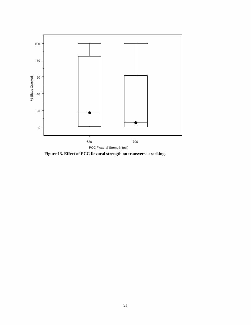
3.1.10 Effect of PCC Flexural Strength

Figure 13 shows that flexural strength of PCC doesn’t have much effect on transverse cracking.

3.1.11 Summary

Figure 14 summarize the effect of different variables on transverse cracking and their relative

importance in controlling cracking. The plots show the average amount of cracking for each factor level of all

the variables. Among the variables that a designer can control, joint spacing and shoulder type have significant

effects on transverse cracking. In general, model predictions for different factor levels of all the variables agree

with prevailing knowledge in pavement engineering. However, there are some exceptions. These anomalies are

discussed in Section 4.

21

626 700

PCC Flexural Strength (psi)

0

20

40

60

80

100

% S

labs

Cra

cked

Figure 13. Effect of PCC flexural strength on transverse cracking.

22

1020

3040

50

% S

labs

Cra

cked

Factors

Mountain

South Coast

Valley7

8

9

10

12

12

13

16

AsphaltShoulder

Tied

WidenedLane

626

700

ClimateRegion

PCCThickness (in.)

TI ShoulderType

PCCStrength (psi)

RuralUrban

ACB

CT B

CH

SP

15

19

LoadSpectrum

BaseType

JointSpacing (ft.)

SubgradeType

Figure 14. Relative effect of all variables on transverse cracking.

23

3.2 Effect of Variables on Faulting

The most important factor controlling faulting is dowels, as shown in Figure 15. Among the three

climate zones, the south coast climate zone shows the least faulting with mountain and valley climate zones

having slightly greater faulting. Structures in mountain and valley climate zones have similar faulting values.

Figure 16 summarizes the effect of climate zones on faulting. As thickness of the PCC slab increases, faulting

decreases as shown in Figure 17. As traffic volume increases faulting increases, as shown in Figure 18. This

figure shows wide truck lanes reduce faulting as well as help in controlling transverse cracking (see Figure 5

for effect of shoulder type on cracking). Figure 19 shows the effect of shoulder types on faulting. The effect of

joint spacing is shown in Figure 20, which shows less faulting with 15-ft. joint spacing than with 19-ft. joint

spacing. Base type, subgrade type, load spectra, and strength of PCC slab don’t have much effect on faulting as

shown in Figures 21, 22, 23, and 24, respectively.

No Dowels Dowels

Dowels

0.0

0.2

0.4

0.6

0.8

Faul

t (in

.)

Figure 15. Effect of dowels on faulting.

24

Mountain(Reno)

South Coast(Los Angeles)

Valley(Sacramento)

Climate Region

0.0

0.2

0.4

0.6

0.8

Faul

t (in

.)

Figure 16. Effect of climate region on faulting.

1210987

PCC Thickness (in.)

0.0

0.2

0.4

0.6

0.8

Faul

t (in

.)

Figure 17. Effect of PCC thickness on faulting

25

12 13 16

TI

0.0

0.2

0.4

0.6

0.8

Faul

t (in

.)

Figure 18. Effect of traffic index (TI) on faulting.

AsphaltShoulder

Tied WidenedLane

Shoulder Type

0.0

0.2

0.4

0.6

0.8

Faul

t (in

.)

Figure 19. Effect of shoulder type on faulting.

26

15 19

Joint Spacing (ft.)

0.0

0.2

0.4

0.6

0.8

Faul

t (in

.)

Figure 20. Effect of joint spacing on faulting.

ACB CTB

Base Type

0.0

0.2

0.4

0.6

0.8

Faul

t (in

.)

Figure 21. Effect of base type on faulting.

27

CH SP

Subgrade Type

0.0

0.2

0.4

0.6

0.8

Faul

t (in

.)

Figure 22. Effect of subgrade on faulting.

Rural Urban

Load Spectra

0.0

0.2

0.4

0.6

0.8

Faul

t (in

.)

Figure 23. Effect of load spectra on faulting.

28

626 700

28-day Flexural Strength of PCC (psi)

0.0

0.2

0.4

0.6

0.8

Faul

t (in

.)

Figure 24. Effect of PCC flexural strength on faulting.

Figure 25 summarize the effect of all the variables considered in the sensitivity study on faulting and

their relative importance. The plots show the average amount of faulting for each factor level of all the

variables. The plots show that faulting is mainly controlled by dowels. Among the variables that can be

controlled by the designer, shoulder type and PCC thickness have significant effects on faulting. There are

some anomalous cases with respect to faulting and these will be discussed in the next chapter.

3.3 Effect of Variables on IRI

In this study, faulting and cracking models are run separately. Subsequently, predicted values of

faulting and transverse cracking are plugged into Equation 1 and Equation 2 to estimate spalling and IRI.

29

0.02

0.04

0.06

0.08

0.10

0.12

0.14

Mea

n of

Fau

lt (in

.) Mountain

South Coast

Valley

7

8

9

10

12

No Dowels

Dowels

AsphaltShoulder

Tied

WidenedLane

12

13

16

Dowels

Factors

ClimateRegion

PCCThickness (in.)

ShoulderType

PCCStrength (psi)

LoadSpectrum

BaseType

JointSpacing (ft.)

TISubgradeType

Rural

Urban

626

700 ACB

CTB

CH

SP

15

19

Figure 25. Relative effect of all variables on faulting.

30

These empirical equations are mentioned in the Design Guide’s user manual.

( ) ⎥⎦⎤

⎢⎣⎡+⎥⎦

⎤⎢⎣⎡

+= +×− SCFAGEAGE

AGESPALL 12005.11100

01.0 (1)

where: SPALL = percentage joints spalled (medium and high severities) AGE = pavement age since construction, years, as shown in Equation 1a SCF = scaling factor based on site, design and climate related variables, as shown

in Equation 1b. ( )( ) 6

200 1015556.01 −∗+∗+ PFIAGE (1a)

where: AGE = pavement age, yr. FI = freezing index, ºF–days P200 = percent subgrade material passing No. 200 sieve

RatioWChAGEFTCYC

fPREFORMAIRSCF

PCC

c

_53643)(2.04.04.3)5.0(%3501400 '

−+×−×++××+−=

(1b)

where: AIR% = PCC air content, percent AGE = time since construction, years PREFORM = 1 if preformed sealant is present; 0 if not f'c = PCC compressive strength, psi FTCYC = average annual number of freeze thaw cycles hPCC = PCC slab thickness, in. WC_Ratio = PCC water/cement ratio

SFCTFAULTCSPALLCCRKCIRIIRI i ∗+∗+∗+∗+= 4321 (2)

where: IRI = predicted IRI, in./mi. IRIi = initial smoothness measured as IRI, in./mi. CRK = percent slabs with transverse cracks (all severities) SPALL = percentage of joints with spalling (medium and high severities) TFAULT = total joint faulting cumulated per mi., in. C1 = 0.8203 C2 = 0.4417 C3 = .4929 C4 = 25.24 SF = site factor

The spalling values estimated using Equation 1 were on the order of 10-9 and 10-10 and hence are not

discussed any further in this report.

Figures 26 to 35 show the effect of different variables on IRI. The variables that affect the IRI most

are the same ones that affect faulting and cracking significantly. So, dowels, traffic volume, joint spacing, PCC

thickness, climate zone, and shoulder type have a significant effect on IRI. On the other hand, base type,

31

subgrade type, and strength of PCC have little effect on IRI. In the following plots it can be seen that the

maximum IRI goes up to 500in./mi. (current Caltrans IRI limit is 224 in./mi. or 3.53 m/km). The cases that

correspond to such high IRI values are those structures that have one or more combinations of high traffic, no

dowels, thin PCC slabs, and 19-ft. joint spacing.

PCC Thickness (in.)

07 8 9 10 12

100

200

300

400

500

IRI (

in/m

ile)

Figure 26. Effect of PCC thickness on IRI.

32

AsphaltShoulder

Tied WidenedLane

Shoulder Type

0

100

200

300

400

500

IRI (

in./m

ile)

Figure 27. Effect of shoulder type on IRI.

12 13 16

TI

0

100

200

300

400

500

IRI (

in./m

ile)

Figure 28. Effect of traffic index (TI) on IRI.

33

No Dowels Dowels

Dowels

0

100

200

300

400

500

IRI (

in./m

ile)

Figure 29. Effect of dowels on IRI.

15 19

Joint Spacing (ft.)

0

100

200

300

400

500

IRI (

in./m

ile)

Figure 30. Effect of joint spacing on IRI.

34

Rural Urban

Load Spectra

0

100

200

300

400

500

IRI (

in./m

ile)

Figure 31. Effect of load spectra on IRI.

ACB CTB

Base Type

0

100

200

300

400

500

IRI (

in./m

ile)

Figure 32. Effect of base type on IRI.

35

CH SP

Subgrade Type

0

100

200

300

400

500

IRI (

in./m

ile)

Figure 33. Effect of subgrade type on IRI.

626 700

28-day PCC Flexural Strength (psi)

0

100

200

300

400

500

IRI (

in./m

ile)

Figure 34. Effect of PCC flexural strength on IRI.

36

Mountain(Reno)

South Coast(Los Angeles)

Valley(Sacramento)

Climate Region

0

100

200

300

400

500

IRI (

in./m

ile)

Figure 35. Effect of climate region on IRI.

Figure 36 summarizes the relative importance of all the variables on IRI. IRI is more sensitive to the

faulting term than the transverse cracking term. The plots show the average IRI for each factor level of all the

variables. Among the factors which a designer can control, dowels (which essentially control faulting) affect

the IRI most, followed by PCC thickness, shoulder type, and joint spacing

3.4 Comparison of IRI Models from 2002DG and Ripper Study

The IRI equation from the Ripper Study is shown in Equation 3.(4)

36 *28.2*84.1*6098.26.99 TcrackeSpallFaultTIRI −+++= (3)

where: FaultT = is total transverse joint faulting (inches/mile) Spall = is percentage of spalled joints, and Tcrack = is number of transverse cracks per mile

37

Rural

Urban 626

700

ACB

CTB

CHSP

15

19

LoadSpectra

PCCStrength (psi)

BaseType

SubcradeType

JointSpacing (ft.)

100

120

140

160

Mea

n of

IRI (

in./m

ile)

Factors

Mountain

SouthCoast

Valley

7

8

9

10

12

12

13

16

No Dowels

Dowels

AsphaltShoulder

Tied

WidenedLane

ClimateRegion

Thickness(in.)

TI Dowels ShoulderType

Figure 36. Relative effect of all variables on IRI.

38

In estimating IRI using the 2002DG IRI model, an initial IRI of 63 in./mile was used so Equation (3)

is modified to use an initial IRI of 63 in./mile, as shown in Equation (4).

36 *28.2*84.1*6098.263 TcrackeSpallFaultTIRI −+++= (4)

Equation (2) shows the IRI model used by 2002DG. It has a site factor term (SF) that depends on the

age, subgrade type, and location of the pavement structure. So, in estimating the IRI using 2002DG model, the

highest and lowest possible values for the site factor were chosen. The highest site factor value corresponds to

CH subgrade (P200 = 75) and Reno climate zone (Freezing Index is 340ºF–days); the lowest value

corresponds to Sacramento climate zone (Freezing Index is 0ºF–days) and SP subgrade (P200 = 10). IRI

predictions are evaluated for gradually progressing distresses of cracking, faulting, and spalling until each of

the distresses reaches its maximum or terminal value. Predicted IRI values using the modified Ripper model

[Equation (4)] and the 2002DG model [Equation (2)] are shown in Figure 37.

Figure 37 shows that the initial predictions from 2002DG and the modified Ripper model match very

well but predictions start diverging as the distresses continue to increase. The modified Ripper model predicts

much higher IRI than the 2002DG model. The current terminal IRI for Caltrans is 224 in./mile. Within this

range, the predictions from both the models are similar. Figure 37 also shows that site factor doesn’t have

much affect on the IRI.

3.5 Effect of Coefficient of Thermal Expansion on Transverse Cracking, Faulting, and IRI

Coefficient of thermal expansion (COTE) was not included in the sensitivity study initially. However,

a separate sensitivity study was performed in order to check the sensitivity of cracking and faulting models to

COTE. Table 4 shows the experimental design used for this satellite sensitivity study.

39

0

100

200

300

400

500

600

700

800

0%, 0

in.,

0%

0.5%

, 0 in

.,0%

1%, 0

.015

in.,

2.5%

5%, .

03 in

., 5%

10%

, 0.1

in.,

25%

20%

, 0.1

7 in

., 25

%

40%

, 0.2

5 in

., 25

%

60%

, 0.3

5 in

., 25

%

80%

, 0.5

in.,

25%

100%

, >0.

6 in

., 25

%

Distress Combination [Cracking (%), Faulting (in.), Spalling (%)]

IRI (

in./m

ile)

IRI_ripper(modified)2002DG(High SF)2002DG(Low SF)

Figure 37. Comparison of IRI models from 2002DG and Ripper study.

Table 4 Experiment Design to for Study of the Effect of the Coefficient of Thermal Expansion (COTE)

Variable Factor Levels

1 COTE (2) 4 × 10-6/ºF7 × 10e-6/ºF

2 Axle Load Spectra (2) Urban Rural

3 Traffic Volume (1) TI: 16

4 PCC Thickness (2) 9 in. 12 in.

5 Base Type (1) Cement Treated Base

6 Dowels (2) Dowels No Dowels

7 Shoulder Type (3) Asphalt Shoulders Tied Shoulders Widened Truck Lane

8 Joint Spacing (2) 15 ft. 19 ft.

9 Climate Regions (3) Mountain Valley South Coast

10 Subgrade Type (1) SP 11 Strength (1) 626 psi Total Number of Cases: 288

40

A COTE of 4 × 10-6/ºF corresponds to PCC mix with limestone or granite aggregate; a COTE of 7 ×

10-6/ºF corresponds to PCC mix with Quartzite, cherts. and gravels. All the cases were run at a reliability level

of 50% and for a design life of 30 years. Figures 38 and 39 summarize the effect of COTE on cracking and

faulting respectively. It can be seen that COTE significantly affects transverse cracking more than it affects

faulting.

3.6 Summary of Sensitivity Analysis Results

Table 5 summarizes the effects of all the variables used in the sensitivity analysis. The table shows the

mean values of transverse cracking, faulting, and IRI for each variable and each factor levels.

Though on an average the model predictions seem reasonable, some anomalies exist, as described in

Section 4.

4 7

COTE (× 10-6/ºF)

0

20

40

60

80

100

% S

labs

Cra

cked

Figure 38. Effect of COTE on transverse cracking.

41

0.0

0.2

0.4

0.6

Faul

itng

(in.)

4 7

COTE (× 10-6/ºF) Figure 39. Effect of COTE on faulting.

42

Table 5 Mean Results of Sensitivity Analysis for Each Variable and Factor Level

Variable Factor Level

Transverse Crack (% Slabs Cracked) Fault (in.) IRI (in./mile)

No Dowels 34 0.15 160 Load Transfer Efficiency Dowels 34 0.01 94

15 ft 15 0.07 111 Joint Spacing (ft.) 19 ft 52 0.09 144 7 in. 52 0.12 159 8 in. 43 0.10 142 9 in. 34 0.08 127 10 in. 26 0.07 114

Thickness (in.)

12 in. 13 0.04 93 Mountain (Reno) 44 0.09 144 South Coast (Los Angeles) 7 0.06 95 Climate Region

Valley (Sacramento) 51 0.09 143 CH 32 0.08 129 Subgrade SP 36 0.07 125 ACB 37 0.09 132 Base Type CTB 30 0.08 122 626 psi 38 0.07 129 PCC Strength 700 psi 29 0.08 125 Asphalt Shoulder 43 0.10 144 Wide Truck Lane 25 0.06 108 Shoulder Tied Shoulders 33 0.09 130 12 21 0.04 98 13 29 0.06 112 Traffic Index 16 51 0.15 171 Urban 34 0.08 125 Load Spectra Rural 33 0.09 129

43

4. ANOMALIES IN THE PREDICTIONS

4.1 Shortwave Surface Absorptivity

Surface absorptivity (SA) is one of the surface properties required by the 2002DG software. SA is

defined as the amount of solar radiation absorbed by the pavement surface. Though this variable was not

included in the sensitivity study presented in this report, it was found that the cracking model is highly

sensitive to SA. A separate experiment was run to understand the sensitivity of the 2002DG models to this

variable. The experiment design for the evaluation of SA was similar to the one used for the main sensitivity

study, but with fewer variables. The variables and factor levels are shown in Table 6.

Table 6 Experiment Design for Study of the Effect of Surface Absorptivity Variable Factor Levels 1 Axle Load Spectra (2) Urban

Rural 2 Traffic Volume (2) TI: 12

14 3 PCC Thickness (3) 8 in.

10 in. 12 in.

4 Base Type (2) Asphalt Concrete Base Cement Treated Base

5 Dowels (2) Dowels No Dowels

6 Shoulder Type (3) Asphalt Shoulders Tied Shoulders Widened Truck Lane

7 Joint Spacing (2) 15 ft. 19 ft.

8 Surface Absorptivity (SA) (2) 0.65 0.85

9 Subgrade Type (1) SP 10 Strength (1) 626 psi Total Number of Cases: 576 Two different values of surface absorptivity, 0.65 and 0.85, are used for surface absorptivity study.

The models in the software were calibrated with a SA value of 0.85 fixed and is not measured for calibration

sections. In the main sensitivity analysis SA was assumed to be 0.65.

Only desert climate, one subgrade type, and one PCC strength were used as opposed to the two values

that were used in the main sensitivity study. All cases were run at a reliability level of 50% and for a design

life of 30 years. After running the cases, it was found that faulting is not much affected by SA. However, some

cases were found for which there is a significant difference in cracking even when every other factor is the

same except surface absorption values. In some cases cracking increased by as much as 17 times when the

44

surface absorption was changed from 0.65 to 0.85. Figure 40 shows a case for which a significant increase in

cracking is predicted due to change in the surface absorption value. The inputs corresponding to this case are:

urban load spectra, 15-ft. joint spacing, wide truck lane, cement treated base, 8-in. PCC slab, design life of 30

years, and a reliability level of 50%.

A closer look at the results from the SA sensitivity study revealed that the thinner pavement sections

were more affected by surface absorptivity. Pavement sections that already have a high amount of cracking

with a SA value of 0.65 are not affected much when SA is changed to 0.85. Figures 41 and 42 summarize the

effect of SA on cracking and faulting, respectively. Figures 43 and 44 show the effect of SA on cracking and

faulting in comparison to the other key variables that affect these distresses. It can be seen that according to

2002DG, SA is as important as traffic volume and shoulder type in its impact on transverse cracking.

0 50 100 150 200 250 300 350Age (months)

0

20

40

60

80

SA 0.65SA 0.85

% S

labs

Cra

cked

Figure 40. Effect of surface absorptivity on transverse cracking, an example.

45

0.65 0.85

Surface Absorptivity

0

20

40

60

80

100

% S

labs

Cra

cked

Figure 41. Effect of surface absorptivity on transverse cracking.

0.65 0.85

Surface Absorptivity

0.00

0.05

0.10

0.15

0.20

0.25

Faul

ting

(in.)

Figure 42. Effect of surface absorptivity on faulting.

46

30

40

50

60

70

80

% S

labs

Cra

cked

Factors

AsphaltShoulder

Tied Shoulder

Wide TruckLane

12

14

8

10

12

15

19

0.65

0.85

Shoulder Type TI PCCThickness (in.)

JointSpacing (ft.)

SurfaceAbsorptivity

Figure 43. Effect of surface absorptivity on transverse cracking compared to other variables.

0.00

0.02

0.04

0.06

Faul

ting

(in.)

Factors

AsphaltShoulder

TiedShoulder

WideTruckLane

12

14

8

10

12

15

19

0.65

0.85

No Dowels

Dowels

ShoulderType

TI Thickness(in.)

JointSpacing (ft.)

SurfaceAbsorptivity

Dowels

Figure 44. Effect of surface absorptivity on faulting compared to other variables.

47

4.2 Cases for which Thinner Pavement Sections Perform Better Than Thicker Sections

There are many cases for which thinner pavement sections had less cracking and faulting when

compared with thicker pavement sections. The following sections present some details of these conditions.

4.2.1 Cases for which Structures with 7-in. Slabs Perform Better Than Those with 8-in. Slabs

Some cases exist for which 7-in. slabs perform better than 8-in. slabs in terms of cracking and

faulting. Out of all the sensitivity runs (8,640 cases), 126 cases showed 7-in. slabs perform better than 8-in.

slabs in terms of cracking and 136 cases showed the same for faulting. In most of these anomalous cases, the

difference in distresses between 7-in. and 8-in. slabs is not much, with a maximum difference in percent slabs

cracked being 12.5% and maximum difference in faulting being 0.27 inches. The second highest difference in

faulting is 0.059 inches. Most of the anomalous cracking cases have the SP subgrade type and 19-ft. joint

spacing. Most of the anomalous faulting cases have CH subgrade.

4.2.2 Cases for which Structures with 8-in. Slabs Perform Better Than Those with 9-in. Slabs

Some cases exist for which 8-in. slabs perform better than 9-in. slabs in terms of cracking and

faulting. In about 12 cases, 8-in. slabs have less cracking than 9-in. slabs with the maximum difference in

percent slabs cracked being 28.4%. The inputs that are common to these 12 cases are:

1. Asphalt concrete base

2. High plasticity clay (CH) subgrade

3. Mountain climate zone

4. 28-day PCC flexural strength of 626 psi

5. Widened truck lane

In about 155 cases, 8-in. slabs have more faulting than 9-in. slabs with a maximum difference in

faulting of 0.0064 inches. There are no inputs common to these 155 cases, however, most of them have 19-ft.

joint spacing.

4.2.3 Cases for which Structures with 9-in. Slabs Perform Better Than Those with 10-in. Slabs

There are 12 cases where 9” slabs have more cracking than 10” slabs with the maximum difference in

percent slabs cracked being 18%. The inputs common to these 12 cases are:

1. High plasticity clay (CH) subgrade

2. Mountain climate zone

3. 28-day PCC flexural strength of 626 psi

48

There are 461 cases for which 9-in. slabs have more faulting than 10-in. slabs with a maximum

difference in faulting of 0.008 inches. The only input common to all these 461 cases is that all of them have

dowels.

4.2.4 Cases for which Structures with 10-in. Slabs Perform Better Than Those with 12-in. Slabs

There are 419 cases for which 10-in. slabs have less faulting than 12-in. slabs with a maximum

difference in faulting of 0.014 inches. The only input common to all of these cases is the inclusion of dowels.

There are no cases for which 10-in. slabs perform better than 12-in. slabs in terms of percent slabs cracked.

4.3 Cases for which Structures with Asphalt Shoulders Perform Better Than Structures with Tied Shoulders

Tied shoulders are supposed to perform better than asphalt shoulders in terms of cracking. However,

there are 18 cases in this study for which structures with asphalt shoulders perform better than those with tied

shoulders. The maximum difference in percent slabs cracked is 24.4%. Inputs common to all these cases are:

1. High plasticity clay (CH) subgrade.

2. Mountain climate zone.

3. 28-day PCC flexural strength of 626 psi.

There is only one case for which a structure with asphalt shoulders has less faulting than a structure

with tied shoulders; the difference in faulting in this case is 0.3282 in.

4.4 Cases for which Structures with Asphalt Shoulder Perform Better Than Structures with Widened Truck Lanes

There are six cases for which structures with asphalt shoulders have less cracking than structures with

widened truck lanes, with the difference in the percent slabs cracking of 12.5%, 0.8%, and 0.2% for the six

cases. Three of the cases have dowels and three are undoweled; the cracking values are same for doweled and

undoweled pavements.

Inputs common to all these cases are:

1. High plasticity clay (CH) subgrade

2. Cement treated base,

3. 28-day PCC flexural strength of 626 psi

4. 15-ft. joint spacing

5. 9-in. slabs

6. Rural load spectra

7. Mountain climate zone

49

There is only one case where structures with asphalt shoulders have less faulting than structures with

tied shoulders; for this case, the difference in faulting is 0.1059 in.

4.5 Cases for which Tied Shoulder Structures Perform Better Than Structures with Wide Truck Lanes

There are eight cases for which structures with tied shoulders performed better than structures with

wide truck lanes in terms of cracking. The maximum difference in percent slabs cracked is 32.1%. The inputs

common to these eight cases are:

1. High plasticity clay (CH) subgrade

2. 12-in. slabs

3. Rural load spectra

4. Mountain climate zone

There are no cases for which tied shoulders perform better than wide truck lane in terms of faulting.

4.6 Subgrade

Poorly graded sand (SP) is stiffer than high plasticity clay (CH) so SP is supposed to be associated with better

pavement performance than CH in terms of faulting and cracking. However, there are 2,644 cases where

structures with CH subgrade are predicted to have less cracking than the structures with SP subgrade. There

are no inputs common amongst these 2,644 cases but most of the cases are in the Mountain climate zone. The

difference in percent slabs cracked goes up to as high as 80 percent in some cases but such cases are very few.

On an average there isn’t much difference in cracking performance between the two subgrade types used in

this study.

There are 735 cases where structures with SP subgrade have more faulting than CH subgrade with a

maximum difference in faulting of 0.16 inches. There are no inputs common to these 735 cases.

In order to understand better the effect of subgrade type on rigid pavement performance, a small

sensitivity analysis was done using 2002DG. Table 7 shows some of the key inputs used for this analysis and

Figure 45 shows the structure used for the analysis. A reliability level of 50 percent is used in this study. The

faulting, transverse cracking and IRI values for different cases at the end of thirty-year design life are shown in

Tables 8 and 9.

50

Table 7 Key Inputs Used to Study the Effect of Soil Type

Input Value

Traffic volume 225 million ESALs (TI of 17)

Climate Valley (Sacramento)

Coefficient of thermal expansion 5.5 x 10-6 /oF

Surface absorptivity 0.65

Shoulder type Asphalt shoulders

Soil types GW, SP, CL, CH

PCC slab thickness 9 in., 12 in.

Joint spacing 15 ft.

Base type CTB

Figure 45. Pavement structure used to study the effect of soil type.

Subgrade (CH/CL/SP/GW)

Aggregate Subbase (6 inches)

CTB (6 inches)

PCC slab (9 inches)

51

Table 8 Performance of Structures with Different Soil Types and without Dowels Soil Type Mr (psi) K (psi/in)* Faulting (in) Cracking (% slabs) IRI (in/mile)

GW 40000 900 0.519 97.6 416.1

SP 28000 775 0.478 96.7 394.1

CL 16000 300 0.402 92.6 350.9

CH 8000 180 0.372 89 332.3

Table 9 Performance of Structures with Different Soil Types and with Dowels Soil Type Mr (psi) K (psi/in.)* Faulting (in.) Cracking (% slabs) IRI (in./mile)

GW 40000 900 0.022 97.6 155.7

SP 28000 775 0.022 96.7 155.5

CL 16000 300 0.055 92.6 169.2

CH 8000 180 0.061 89 169.7

CH 5000 125 0.063 83.7 166.1

CH 1000 41 0.084 61 158.5

CH 500 25 0.099 75.1 177.6

* Approximate Dynamic k-value estimated by the software from the Mr value

The predicted faulting and transverse cracking versus age (months) for the pavement analyzed with

the four types of subgrade for no dowels, and the four moduli for the CH subgrade for the doweled pavement,

are shown in Figures 46 through 48.

52

0

0.1

0.2

0.3

0.4

0.5

0.6

0 50 100 150 200 250 300 350 400

Age (months)

Faul

ting

(in)

CHCLSPGW

Figure 46. Faulting for different subgrade types, undoweled pavements.

0

0.02

0.04

0.06

0.08

0.1

0.12

0 50 100 150 200 250 300 350 400

Age (months)

Faul

ting

(in)

CH (Mr-500 psi)CH (Mr-1000 psi)CH (Mr-5000 psi)CH (Mr-8000 psi)CLSPGW

Figure 47. Faulting for different subgrade types, doweled pavements.

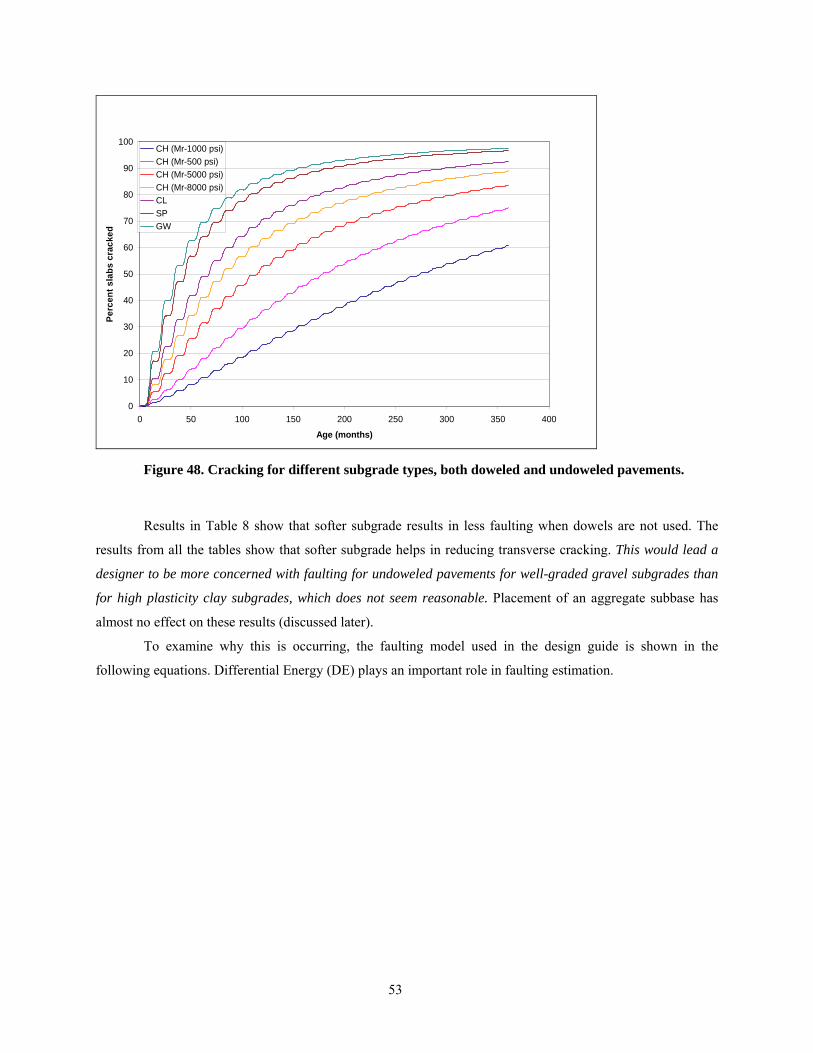
53

0

10

20

30

40

50

60

70

80

90

100

0 50 100 150 200 250 300 350 400

Age (months)

Perc

ent s

labs

cra

cked

CH (Mr-1000 psi)CH (Mr-500 psi)CH (Mr-5000 psi)CH (Mr-8000 psi)CLSPGW

Figure 48. Cracking for different subgrade types, both doweled and undoweled pavements.

Results in Table 8 show that softer subgrade results in less faulting when dowels are not used. The

results from all the tables show that softer subgrade helps in reducing transverse cracking. This would lead a

designer to be more concerned with faulting for undoweled pavements for well-graded gravel subgrades than

for high plasticity clay subgrades, which does not seem reasonable. Placement of an aggregate subbase has

almost no effect on these results (discussed later).

To examine why this is occurring, the faulting model used in the design guide is shown in the

following equations. Differential Energy (DE) plays an important role in faulting estimation.

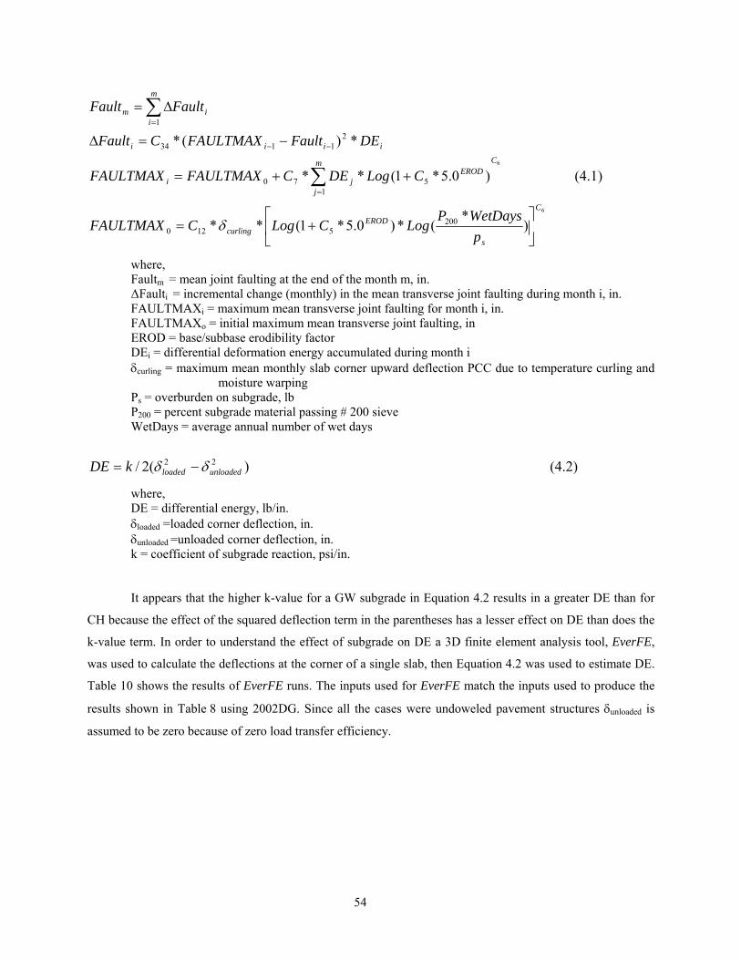
54

6

6

)*

(*)0.5*1(**

(4.1) )0.5*1(**

*)(*

2005120

1570

21134

1

C

s

ERODcurling

Cm

j

ERODji

iiii

m

iim

pWetDaysP

LogCLogCFAULTMAX

CLogDECFAULTMAXFAULTMAX

DEFaultFAULTMAXCFault

FaultFault

⎥⎦

⎤⎢⎣

⎡+=

++=

−=Δ

Δ=

∑

∑

=

−−

=

δ

where, Faultm = mean joint faulting at the end of the month m, in. ΔFaulti = incremental change (monthly) in the mean transverse joint faulting during month i, in. FAULTMAXi = maximum mean transverse joint faulting for month i, in. FAULTMAXo = initial maximum mean transverse joint faulting, in EROD = base/subbase erodibility factor DEi = differential deformation energy accumulated during month i δcurling = maximum mean monthly slab corner upward deflection PCC due to temperature curling and

moisture warping Ps = overburden on subgrade, lb P200 = percent subgrade material passing # 200 sieve WetDays = average annual number of wet days

(4.2) )(2/ 22unloadedloadedkDE δδ −=

where, DE = differential energy, lb/in. δloaded =loaded corner deflection, in. δunloaded =unloaded corner deflection, in. k = coefficient of subgrade reaction, psi/in.

It appears that the higher k-value for a GW subgrade in Equation 4.2 results in a greater DE than for

CH because the effect of the squared deflection term in the parentheses has a lesser effect on DE than does the

k-value term. In order to understand the effect of subgrade on DE a 3D finite element analysis tool, EverFE,

was used to calculate the deflections at the corner of a single slab, then Equation 4.2 was used to estimate DE.

Table 10 shows the results of EverFE runs. The inputs used for EverFE match the inputs used to produce the

results shown in Table 8 using 2002DG. Since all the cases were undoweled pavement structures δunloaded is

assumed to be zero because of zero load transfer efficiency.

55

Table 10 DE Estimation Based on EverFE Runs

Soil Type K(psi/in.) δloaded (in.) δunloaded (in.)

DE (lb-in.)

per Equation 4.2

CH 180 0.040 0 0.144

CL 300 0.027 0 0.109

SP 775 0.013 0 0.065

GW 900 0.012 0 0.064

According to EverFE, as the stiffness of the subgrade increases the differential energy decreases so

faulting is supposed to decrease. However, in the 2002DG DE increases as the stiffness of the subgrade

increases. This is shown in Figure 49. The figure also shows that the DE values are on order of few hundreds

in magnitude of (lb-in.) whereas EverFE estimation of DE results in values less than 1 for DE. The reasons for

this large a difference are not known. EverFE and ISLAB2000 have generally been shown to have similar

results.

0

100

200

300

400

500

600

700

800

0 50 100 150 200 250 300 350 400

Pavement Age (monts)

Diff

eren

tial E

nerg

y (lb

-in)

CHCLSPGW

Figure 49. Effect of subgrade on DE for undoweled pavements according to 2002DG.

The only other variable directly affected by the subgrade in the faulting equation is the percentage of

material passing the No. 200 sieve (P200 in Equation 4.1). The default values for the subgrade types were used

for this analysis.

56

Table 11 Default P200 Values Used in the Study Soil Type P200

CH 75

CL 75

SP 10

GW 5

Although the calculations in the software are not transparent, it appears that the P200 did not have

much effect on the predicted faulting. A couple of cases have been run with CH subgrade varying P200 values,

and the effect of P200 was found to be insignificant. The results are shown in Table 12.

Table 12 Effect of P200 on Faulting, Cracking, and IRI for Undoweled Pavements P200 Faulting (in.) Transverse

Cracking (%)

IRI (in./mile)

50 0.399 92.7 349.4

75 0.402 92.6 351.7

100 0.404 92.5 351.9

The Valley climate region is hot, which induces a great deal of curl, but it has almost no summer rainfall. The

effect of the wet days variable cannot be directly changed in the software and its effect on faulting could not be

studied. However, it appears from the equation that the faulting model may not be very sensitive to the number

of wet days.

4.7 High K-value of Subgrade

It is observed that in cases with SP subgrade, the k-value of the subgrade estimated by the software

(from the default E value of 28,000 psi) is about 800 psi/in., which is very high. The software doesn’t allow

direct input of the k-value of the subgrade, and instead it is computed from the E value of the subgrade.

Discussions with one of the developers of the rigid module of the 2002DG software indicated that the

maximum k-value used in developing the models was about 500 psi. This may partly explain some of the

anomalies.

A few cases were rerun to see if the discrepancy in the value of the surface absorptivity used could

explain the anomalies, but the same trend continued even with a surface absorptivity value of 0.85.

57

5. LIMITATIONS AND BUGS IN THE SOFTWARE

5.1 Inability to Reproduce Results

For some projects, it was found that two input files containing the same data produced totally different

outputs. This occurs when the file is saved using the ‘Save As’ option in the File menu of the software.

However, this doesn’t happen every time the ‘Save As’ option is used. This problem was detected for only a

very few cases. Cases for which this problem was observed showed unreasonable results, such as 0% cracking

for 7-in. slabs with 19-ft. joint spacing under very high traffic volume. When such cases were re-run with the

same input files, they gave different results that were reasonable. After identifying this problem, many cases

were selected randomly and were rerun to double-check the results. Almost all of them produced consistent

results. One variable that is common among all cases where results could not be reproduced is slab thickness of

7 in.

5.2 Base Properties

When the base type is changed, the default input values are not changed. Irrespective of the base type

chosen, the same default values for elastic modulus, unit weight, and thermal properties are assigned. An

example is shown in Figure 45. Generally, when the user changes the base type, the program automatically

changed thickness to zero or to a very low number. In addition, once some changes are made they cannot be

discarded by clicking on the ‘Cancel’ button. Figure 46 shows that in spite of clicking on the ‘Cancel’ button,

base type is changed as shown in Figure 45.

58

Figure 45. Base Properties input screen shots

59

Figure 46. Structure window screen shot.

5.3 Aggregate Type

The type of aggregate is a redundant input as it does not effect the calculations of the distresses. When

aggregate type is changed, the coefficient of thermal expansion of PCC is not changed automatically—it must

be changed manually. Also, other mix properties like PCC zero-stress temperature are not changed when the

user changes the aggregate type.

5.4 Climate Data

Some major California weather stations are not in the list of weather stations for which the software

has climate data. Some stations in the software’s list don’t have more than two years of data. If chosen, some

weather stations in the software list result in errors and the program shuts down. For example, Eureka is a

major weather station in California but the software has only 11 months of climate data. Because it has only 11

months of data, the software cannot be run. The software requires more than 12 months of data to run. Ukiah is

another major weather station in California but the software has only 12 months of data for this station

[Climate Database for Integrated Model (CDIM) has more 30 years of data for both Ukiah and Eureka].

Cases utilizing the Ukiah climate file can be run, but the software stops while running showing the

error message shown in Figure 47. Such problems cast a doubt on the credibility of the climate database in the

software. Also, when such error messages are encountered it is very hard to identify the input that caused the

error.

60

Figure 47. Error message when Ukiah climate file was used.

5.5 Running the Software in Batch Mode

The software provides the option of running several projects in a batch mode. This can be done by

clicking on the ‘Tools’ tab and then clicking ‘Batch File.’ When this is done, a window opens allowing the

user to enter file names of all the projects to run in batch mode. Figure 48 shows a batch file window where

several projects are selected to run in batch mode. However, as seen in the figure, the ‘Run’ tab is not

highlighted, so the user cannot use the batch mode option.

5.6 Spalling Not Included in Output

Spalling is estimated by the software using an empirical model [see Equation (1) in Chapter 3] but the

estimated spalling values are not shown in software output.

61

Figure 48. Batch file window.

5.7 Other Problems

The software occasionally shuts down while running. After the software shuts down and is reopened,

the program sometimes goes into ‘debug mode.’ The program then opens windows with confusing messages

and values could not be input to the software. Some of these windows are shown in Figures 49-52. This

problem occurred three times during the sensitivity study. After each occurrence, the software had to be

reinstalled in order to run again.

Figure 49. Error message.

62

Figure 50. Debug mode.

63

Figure 51. Screen shot showing that inputs could not be entered.

Figure 52. Error message when PCC thickness is chosen as 10 in.

64

6. CONCLUSIONS

Sensitivity analysis done as part of this study helped to identify the basic behavior of the models and

to identify some flaws in the 2002DG models and the software. From all the cases run as part of this study, the

following conclusions have been drawn:

1. In spite of requiring a large number of inputs, the software is very user-friendly with very useful

help files.

2. Some of the inputs required by the software are hard to obtain so the designer has to rely on

default values suggested by the Design Guide or use approximate values. Some of the inputs for

which default values are assumed have significant impact on predicted performance.

3. On average, both the cracking and faulting models show trends that agree with prevailing

knowledge in pavement engineering. According to 2002DG, transverse cracking is sensitive to

surface absorptivity, coefficient of thermal expansion, joint spacing, shoulder type, PCC

thickness, traffic volume, and climate zone. Faulting, according to 2002DG, is sensitive to

dowels, traffic volume, thickness, shoulder type, and climate zone.

4. There are some specific cases for which the models predict results that do not agree with

accepted pavement knowledge. Anomalies, applicable to both transverse cracking and faulting

models, are :

1. Some thinner pavement structures perform better than thicker pavement structures

2. Some structures with asphalt shoulders perform better than structures with tied shoulders and

widened truck lanes

3. Some structures on CH subgrade perform better than structures on SP subgrade.

4. Surface absorptivity is predicted to have a tremendous effect on cracking performance in some

cases. However, it is difficult to find commonalities in these cases. Results show that cases with

thinner pavement structure are most affected by changes in surface absorptivity.

5. Subgrade k-value in many cases is unusually high when SP subgrade is used. This suggests there

may be some flaws in the ‘E-to-k’ conversion model used in the software.

6. Inability to reproduce the results can confound the credibility of model predictions. This occurred

when two input files containing the same data produced totally different outputs. Fortunately, in

the current study it was easy to identify such cases because they predicted 0% cracking when they

were expected to crack substantially and there were very few such cases. A small percentage of

cases were re-run and they all yielded consistent and reasonable results.

7. Some major weather stations in California are not included in the climate database built into the

software. Some of the climate files are corrupt and cause the software to crash.

65

8. PCC properties like coefficient of thermal expansion are not changed automatically when the user

changes aggregate type, making it a redundant variable.

9. The software occasionally crashes and needs to generally be more robust.

This study is by no means exhaustive. A couple of related sensitivity studies have been performed to

evaluate the impact of some of the variables that were not included in the main experiment design. There could

still be some flaws that were unidentified and there still could be some variables that seem very innocuous but

have significant impact on cracking and faulting models. Overall the rigid part of the 2002DG produces

reasonable predictions of pavement performance. However, the accuracy of the predictions needs to be

validated by using field data in California. If 2002DG needs to be used for pavement design, it should be used

with some caution, keeping in mind the anomalies mentioned in the report.

66

7. REFERENCES

1. Pomerantz, M., B. Pon. The Effects of Pavements’ Temperatures on Air Temperatures in Large Cities. Lawrence Berkeley National Laboratory, Berkeley, California, April 2000.

2. Mancio, M., J. T. Harvey, A. Ali, J. Zhang. Evaluation of the Maturity Method for Flexural Strength Estimation in Concrete Pavement Draft report prepared for the California Department of Transportation. Pavement Research Center, University of California. May 2004.

3. du Plessis, L., F. Jooste, S. Keckwick, W. Steyn. Summary Report of HVS Testing of the Palmdale Test Site, North Tangent Sections: Evaluation of Long Life Pavement Rehabilitation Strategies—Rigid. Draft report prepared for the California Department of Transportation, CSIR Transportek, Pretoria, Republic of South Africa; Pavement Research Center, Institute of Transportation Studies, University of California Berkeley, University of California Davis, August 2005.

4. Yu, H., M. Darter, K. Smith, J. Jiang and L. Khazanovich, “Performance of Concrete Pavements, Volume III – Improving Concrete Pavement Performance,” Final Report, Contract No. DTFH61-C-00053, Federal Highway Administration, McLean, Virginia, 1996.

67

8. APPENDIX A: SCREEN SHOTS FROM THE SOFTWARE

Figure A1. General Traffic Inputs (Number Axles/Truck tab)

Number of axles per truck information is obtained from WIM data. Default values have been used for mean wheel location, traffic wander standard deviation, and design lane width.

68

Figure A2. General Traffic Inputs (Axle Configuration tab)

Default values have been used.

69

Figure A3. General Traffic Inputs (Wheelbase tab).

Wheel base information is obtained from WIM data.

70

Figure A4. JPCP Design Features.

Screen shot of design features inputs. It is assumed that there is no bonding between PCC and base.

71

Figure A5. PCC Material Properties (Thermal properties tab).

72

Figure A6. PCC Material Properties (Mix properties tab).

73

Figure A7. PCC Material Properties (Strength tab).

74

Figure A8. Asphalt Material Properties (Asphalt Mix tab).

75

Figure A9. Asphalt Material Properties (Asphalt Binder tab).

76

Figure A10. Asphalt Material Properties (Asphalt General tab).

77

Figure A11. Cement/Lime Stabilized Material (Cement Stabilized option).

78

Figure A12. Unbound Layer #3 (Strength Properties tab, A-1-a option).

79

Figure A13. Unbound Layer #3 (ICM tab).

80

Figure A14. Unbound Layer #4 (Strength Properties tab, CH material option).

81

Figure A15. Unbound Layer #4 (Strength Properties tab, SP material option)

82

Figure A16. Unbound Layer #4 (ICM tab, CH material option).

83

Figure A17. Unbound Layer #4 (ICM tab, SP material option).