DISCRETE APPLIED

ELWVIER Discrete Applied Mathematics 55 (1994) 145-162 MATHEMATICS

Sensitivity analysis of list scheduling heuristics

A.W.J. Kolena, A.H.G. Rinnooy Kanb, C.P.M. van Hoeselb-**, A.P.M. Wagelmans b, *

’ University qf’ Limburg. P.O. Bo.u 616. NL-6200 MD Maastricht, Netherlands b Erasmus University Rotterdam, P.O. Bo?c 1738, NL-3000 DR Rotterdam. Netherlands

Received 14 November 1990: revised 12 March 1993

Abstract

When jobs have to be processed on a set of identical parallel machines so as to minimize the makespan of the schedule, list scheduling rules form a popular class of heuristics. The order in which jobs appear on the list is assumed here to be determined by the relative size of their processing times; well-known special cases are the LPT rule and the SPT rule, in which the jobs are ordered according to non-increasing and non-decreasing processing time respectively.

When all processing times are exactly known, a given list scheduling rule will generate a unique assignment of jobs to machines. However, when there exists a priori uncertainty with respect to one of the processing times, then there will be, in general, several possibilities for the assignment that will be generated once the processing time is known. This number of possible assignments may be viewed as a measure of the sensitivity of the list scheduling rule that is applied.

We derive bounds on the maximum number of possible assignments for several list schedul- ing heuristics, and we also study the makespan associated with these assignments. In this way we obtain analytical support for the intuitively plausible notion that the sensitivity of a list scheduling rule increases with the quality of the schedule produced.

Key words: Sensitivity analysis; List scheduling; Heuristics; Robustness; Scheduling

1. Introduction

Combinatorial problems whose computational complexity effectively rules out

their optimal solution within a reasonable amount of time are frequently solved by

heuristics, fast methods that produce a suboptimal, but hopefully reasonable, feasible

solution. The analysis of their performance is a lively research area. In addition to

empirical analysis, the emphasis has mostly been on worst case and probabilistic

*Corresponding author.

**Present address: Eindhoven University of Technology, P.O. Box 513, 5600 MB Eindhoven, The Netherlands.

0166-218X/94/$07.00 0 1994-Elsevier Science B.V. All rights reserved

SD1 0166-218X(93)E0089-H

146 A. W.J. K&n et al. 1 Discrete Applied Mmhemarics 5.5 (1994) 145 162

analysis of the deviation between the heuristic solution value and the optimal

one.

There is, however, an important feature of algorithmic behavior that has hardly

received attention. It concerns the effect on algorithmic performance of perturhutions

in the problem data. This effect has been well studied for optimization methods, under

the general heading of sensitivity analysis or parametric optimizution (for a review see

Wagelmans [S]). Typically, one finds that the optimal solutions to hard (i.e., NP-hard)

optimization problems are highly unstable, in that a small change in the problem data

can produce a large change in the value or structure of the optimal solution. This

characteristic property provides an additional incentive to turn to heuristic methods

in which case a more robust behavior could be hoped for. Indeed, it is plausible to

conjecture an inverse relation between the quality of the solution produced by the

heuristic and its robustness under changes in problem data. At one end of the

spectrum, the optimal solution is very unstable; at the other end, very simplistic

heuristics that extract little information from the data will produce very poor but very

stable solutions. Most heuristics will be somewhere in between the two.

In this paper, we obtain some evidence supporting this general conjecture for the

special case of the minimization of makespan on parallel identical machines. In this

prototypical scheduling problem, n jobs with processing times p, , ..,pn have to be

distributed among m identical machines so as to minimize the time span of the

resulting schedule. If the completion time of the jth job is denoted by Cj, then this

criterion amounts to the minimization of Z = maxi = I,,,,,n{Cj). Note that a solution

corresponds to an assignment ofjobs to machines, because the exact order in which the

jobs are processed on the machines does not matter. Furthermore, since machines are

identical we do not distinguish between them. Therefore, an assignment of jobs to

machines is actually a partition of the jobs into m subsets.

The problem of minimizing makespan on parallel identical machines is NP-hard

and it has been the subject of extensive research; many heuristics for its solution have

been proposed (for a review see Lawler et al. [4]). We will concentrate on a class of

heuristics known as list scheduling rules. Such rules are defined by a priority list on

which the jobs appear in order of decreasing priority. Whenever a machine becomes

idle, the unscheduled job with the highest priority is assigned to this machine.

Depending on the way the priority list is constructed, the schedules produced by such

heuristics may be quite poor or quite good. Thus, this class of heuristics provides

a natural vehicle for the analysis of the relation between solution quality and

robustness.

To arrive at an exact formulation, we restrict our attention to priority lists that are

defined by the relative sizes of the processing times. To be more precise, it is assumed

that the jobs are initially ordered according to non-decreasing processing time, and

a list scheduling rule corresponds to a permutation 7c such that the jth job of this

initial order is always put in the ~(j)th position on the list. Hence, for given n, there

exists a mapping from these permutation list scheduling rules to the elements of S,, the

set of n-permutations. For given n it is actually sufficient to consider only the

A. W.J. Kolrn et ul. ! Disrrrte Applid Mntlwmatic~s 55 (1994) 145-162 147

permutation, i.e., we do not need to know the exact rule by which it was generated.

Therefore, we will often let the permutation represent the list scheduling rule. One

should keep in mind, however, that the permutation that corresponds to a given

permutation list scheduling rule in the case of II jobs, does, in general, not provide any

information about the permutations that the same rule will generate when the number

of jobs is unequal to n. In other words, a permutation list scheduling rule is only

completely specified by a set of permutations, namely one permutation for every

number of jobs.

Two well-known examples of permutation list scheduling rules are the SPT

(Shortest Processing Time) and the LPT (Longest Processing Time) rules, defined

by n(j) =j and n(j) = n -j + 1, j = l,..., n, respectively. The quality of the

solution produced by these rules is very different. The SPT rule yields schedules

whose value can exceed the optimal one by a factor of 2 - l/m (see Graham [2]);

for the LPT rule, this factor is at most $ - 1/(3m) (see Graham [3]); both bounds

are tight. A similar difference in quality emerges from a probabilistic analysis: if

the processing times of the jobs are independent and uniformly distributed, then

it can be shown that the expected absolute error of the LPT rule is 0(1/n), whereas the

expected absolute error of the SPT rule is Q(l) (see Frenk and Rinnooy Kan

Cl]). From now on we assume that the processing times of jobs 2 to n are exactly known

and that pz < p3 d ‘.. d p,, holds. Suppose that, for the time being, there exists

uncertainty with respect to the value of pl. Because of this uncertainty, we do not yet

know how a given list scheduling heuristic will eventually assign the jobs to the

machines. In general, there will be several possibilities for that assignment and which

one will actually be generated depends on the exact value of pl. The total number of

possible assignments can be taken as a measure of the sensitivity of the list scheduling

rule with respect to the value of p,. If this number is low, then this indicates that the

rule is robust, because for many values of p, the same assignment will result. On the

other hand, a high number of possible assignments means that the exact value of p1 is

obviously very important in constructing the solution. Therefore, in the latter case,

the list scheduling rule can be considered sensitive to uncertainty with respect

to Pl.

To be able to say something about the number of possible assignments that can be

generated by a given list scheduling rule when uncertainty exists with respect to one of

the processing times, we will actually carry out a parametric analysis with respect to

pl. This means that we will study the SPT rule, the LPT rule and other permutation

list scheduling rules when p, = 2, where jb gradually increases from zero to infinity.

For a given list scheduling heuristic 7c and given n we define A,” to be the worst case

number of’d$?rent assignments of jobs to machines that occur when 1 increases from

zero to infinity. Besides the number of solutions generated by the list scheduling rule it

is also natural to study the solution value Z:(A) as a function of 2. As we will see in

Section 2, Z,” is a continuous piecebvise linear function. The values of 3, in which this

function is not differentiable are called breakpoints. Note that 0 is a breakpoint. We

148 A. W.J. K&n et al. 1 Discrete Applied Mathematics 55 (1994) 145-162

define B,” to be the worst case number of breakpoints of 2:. This number may serve as

a first indication of how quickly the solution value adapts to changes in the problem

data.

In Sections 3 and 4, we look at the SPT rule and the LPT rule, respectively. We

establish that AfPT d n and BfPT < 2rn/ml; both upper bounds are tight. In contrast ALPT < 2”~” and &.PT < 2”-“+ 1;

foi which BfPT

the first bound is tight, and there exists an example

> 2(“pm)i2. These results nicely support the conjectured relationship

between solution quality and robustness. In Section 5, we show that the LPT rule is

almost an extreme case; for an arbitrary permutation n, A,” d 2n-mf1 and

B,” 6 2npm+2. A summary of the results and some concluding remarks are collected in

Section 6.

2. The function Zi

In this section we show that for any list scheduling rule defined by a permutation

x on the processing times p1 = J. and p2 < p3 < ... < pn, Zi is a continuous piecewise

linear function of i, 0 < 2 < co. Each of the linear parts of Z,” will be constant or have

a slope of one.

To illustrate the result, we first present an example with two machines and four jobs

having processing times p1 = 2, p2 = 1, p3 = 2, p4 = 4, that are scheduled according

to the LPT rule. The different schedules and corresponding linear parts of ZipT are

given in Fig. 1.

Let us now look at an arbitrary permutation list scheduling heuristic applied

to an arbitrary problem instance. When I is increased from zero to infinity

the ordering of the jobs according to non-decreasing processing times will change.

Hence the list will change too, although the relative order of the jobs 2,3, . . . . n will

remain the same. If 2 is equal to one of the processing times p2, . . . , p,,, then we may

assume that in the order according to non-decreasing processing time job 1 follows

directly after the job with largest index for which the processing time equals 1. Thus,

a further increase of i leaves the current ordering unchanged until 1 becomes equal to

the next larger processing time. It is easily verified that Z,” is continuous in J. = pj

(j = 2, . . . . n). To establish our result, it is sufficient to show that when 2 varies between

processing times pj and pj+ 1 with pj < pj+ 1, Z,” is a continuous piecewise linear

function.

Before analyzing Z:(J) for 1~ [pj, pi+ i) we will make one more assumption

about the schedule produced by the heuristic. Consider a job which is after job

1 on the list, and is ready to be scheduled. If there exists a choice of machines to

schedule this job on (i.e., at the same point in time more than one machine becomes

available), we will always choose a machine not containing job 1. This assumption

does not affect the distribution of total processing time among the machines and

therefore it does not affect Z;. Let us refer to this assumption as the tie breaking

assumption.

A. W.J. Kolen et al. 1 Discrete Applied Mathematics 55 (1994) 145-162 149

Ml 4 12)

Mz I 1 1 3 1

Ml 4 I 3 1

M2 I 1 I 2

0 2 x < 1 ZyyX) = 4

1 < x < 2 _ Z‘y(X) = 3 t x

2 < x < 3 = 5 - Z,LPT(X)

3 5 x < 4 ZkPT(X) = 2 t x

4 < X < 5 Z,LpT(X) = 6 _

5<X<6 Z,LPT(X)=ltX

6 < x < 7 Z,LPT(X) = 7

7 < x < co Z‘yT(X) = x _

Fig. 1. Example LPT-schedules

I I I f I I I I I I t I

0 1 2 3 4 5 6 7 8 9 10 11

b e

0 c d I

L ! I I I I I I I I I I 0 1 2 3 4 5 6 7 8 9 10 11

Fig. 2. A switch of tails.

Since we are analyzing Z,” over an interval in which the order of the jobs on the list

remains unchanged, the only way the schedule can be affected is by changes in the

times on which machines become available. This is illustrated in Fig. 2 for the case of

two machines Ml and M,. Assume that the jobs a, b, c, d, e occur on the list in alphabetical order. When the

processing time ofjob 1 is increased by ,U (0 < p < 1) the schedule does not change and

Zz increases linearly with slope one. For p = 1, machines Ml and M2 become

available at the same time, namely at the completion time of job 1. From our tie

breaking assumption, jobs b, e are now scheduled on Ml and jobs a, c, d on M2. Note

that Z; remains the same but the maximum machine, i.e., the machine for which Z,” is

attained, has changed. The motivation for the tie breaking assumption is that an

150 A. W.J. Kolen et al. / Discrete Applied Mathematics 55 (1994) 145-162

Ml Ill m+l I 2m+l

n/i, I 2 I m+2 I

Mm-1 I m-1 I 2m-1 I

M,z I m I 2n I

Fig. 3. SPT-schedule

incremental increase of p will now not affect the schedule. We refer to the transforma-

tion depicted in Fig. 2 as a switch of tails. If p would increase to 4, then another switch

of tails would occur; job e would switch to M2. Note that 2: is constant for 1 d p d 3,

whereas Z,” increases with slope one for 3 d p < 4.

In general, it is easy to see that before a switch of tails occurs Z,” is constant as long

as job 1 is not on the maximum machine. If the machine containing job 1 becomes the

maximum machine, then Z,” increases with slope one. A switch of tails does not affect

the value of the makespan and after a switch Z,” will be constant or increase with slope

one depending on whether or not job 1 is on the maximum machine. This establishes

the desired result.

3. The SPT rule

According to the SPT rule jobs appear on the list in order of non-decreasing

processing time. For n jobs with processing times pi = 2 < pz < ... < pn, the SPT-

schedule is illustrated in Fig. 3. For j = 1, 2, . . . , m we may assume that job j is scheduled

on machinej. Since Mi is the first machine which becomes available again, job m + 1 is

scheduled on M, . Because p1 + pm+ 1 2 pm machine Mi now is the maximum machine

and job m + 2 is scheduled on M2. Since pz z p1 and pm+ 2 3 pm+ 1 machine M2 has

now become the maximum machine and job m + 3 is scheduled on M3. Continuing this

way we find that an SPT-schedule can always be assumed to have the following

structure: job j is scheduled on machine Mi where i is given by i = r( j - l)mod ml + 1,

j=l , . . . , n, and the maximum machine is the machine processing job n. Let us now consider the case that the processing time p1 = 2 is increased from zero to

infinity. It follows from the structure of the SPT-schedule that there will be at most

n different assignments of jobs to machines, and this bound is attained if

P2~P3~“‘~Pn. Hence, AipT = n. On each machine in the SPT-schedule either

rn/mlorrn/ml- 1 ’ b JO s are scheduled. The maximum machine will always be machine

[(n- l)modml+ 1 d’t 1 an 1 a ways contains [n/ml jobs. Therefore job 1 can be on the

maximum machine at most r n/m 1 times. Since ZiPT can only have a slope of one if in the

corresponding interval job 1 is on the maximum machine, it follows that ZzPT has at

A. W.J. Kolen et al. / Discrete Applied Mathematics 55 (1994) 145-162 151

most [n/ml linear parts with slope one. Therefore there can be no more than 2rn/ml

breakpoints of ZtPT. It is easy to see that if we take a problem instance with n mod m # 1

and p2<p3<...<pn, then this upper bound on the number of breakpoints is

attained. Hence, BfPT = 2rn/ml As ZtPT 1s completely determined by its breakpoints

and their function value, we conclude that ZfPT can be computed in polynomial time.

4. The LPT rule

According to the LPT rule, jobs are assigned in order of decreasing processing

times. Again, let us assume that job 1 has processing time A, and that

p2 d p3 d ... d pn.

We first prove that the worst case number of different LPT-assignments, AkPT, is at

most equal to 2”-” for all n 3 m. We do so by induction. For n = m, the statement is

trivial since each machine is assigned exactly one job and we do not distinguish

between machines. Assume that the statement holds for n (n B m), and consider an

instance of the (n + 1)-job problem. Compare this instance to the n-job instance

obtained by deleting job 2. By induction, it is possible to partition the I-axis [0, co)

into at most 2”-” intervals, such that in the interior of each interval the assignment of

jobs to machines for this n-job instance remains the same. We will investigate how the

(n + 1)-job assignments are related to these n-job ones.

To facilitate our analysis we define for the n-job instance the minimum machine to be

the machine with minimal total processing time. QiPT will denote the completion time

of the minimum machine as a function of 2. Analogously to Section 2 one can prove

that QkPT is a continuous piecewise linear function.

Consider the (n -t 1)-job instance. First assume that 2 2 p2. Thus, job 2 is the

smallest one and the LPT rule assigns it (as the last job) to the minimum machine of

the n-job instance. Now consider an arbitrary A-interval in which the assignment of

the n-job instance does not change. What can happen to the minimum machine in the

interior of such an interval? Its index can change only once, namely when the initial

minimum machine contains job 1 and loses its status due to the increase of 2 (the slope

of Qn LPT changes from one to zero). Hence, each such interval generates at most two

intervals for the (n + I)-job instance and the corresponding assignments differ only in

the assignment of job 2.

We now turn to the case that i is less than p2. Let [0, a) be the first A-interval for the

n-job instance. Because the assignment of the n-job instance does not change as long

as 2 is less than the smallest processing time p3, it holds that a 2 p3 B p2. It follows

that [0, p2) is contained in [0, a). Hence, [0, a) is the only interval of the n-job instance

for which we have not proven yet that it corresponds to at most two similar intervals

of the (n + 1)-job instance. To prove that the latter does hold, first note that we have

already observed above that Q,, LPT has at most one breakpoint in (0, a). Furthermore, it

is obvious that the assignment of the (n + 1)-job instance can not change for 2 < p2.

Hence, if QiPT has no breakpoint in (~~,a), then there will be at most two different

152 A. W.J. K&n et al. / Discrete Applied Mathematics 55 (1994) 145-162

/

Ml

M2

b: jobs 1,3,...,n

Pz<X<p

M3

c: jobs 1,2,...,n

PzIX<p

M3

a: jobs 3,4,, . . , n

\

Ml M2

M3

d: jobs 2,3,. . . , n

Ml --2

M3

e: jobs 1,2,...,n

05X<Pz Fig. 4. Schedules for I E [0, p).

assignments of the (n + I)-job instance in [O,a), namely one in each of the intervals

[0,p2) and [p2, a). So we are left with the case that Q iPT has a breakpoint p in (pZ, a).

At first sight there may be three different assignments, corresponding to [0,p2),

[p2, v), and [,u, a). However, we will show that the assignments on [O,pZ) and [pZ,p)

are identical.

In Fig. 4(a) the LPT-schedule of the jobs 3, . . . , n is given, where we have assumed

that machines are numbered such that Mi has no more total processing time assigned

to it than Mi + 1, i = 1, . . . , m - 1. The fact that Q,“” has a breakpoint p E (pZ, a) means

that M1 is the minimum machine as long as the processing time ofjob 1 is less than or

equal to p. Hence, the difference between the total processing time of M, and M2 is

exactly equal to p. The schedule of the n-job instance on [p2, ,u) is given in Fig. 4(b).

The schedule of the (n + l)-job instance on [pZ, n) is obtained from the n-job instance

by scheduling job 2 on the minimum machine M, The schedule is given in Fig. 4(c).

On [O,p,) the schedule of the jobs 2,3, . . . . y1 is given by Fig. 4(d). This schedule is

obtained from the schedule in Fig. 4(a) by scheduling job 2, which is smallest among

the jobs we consider at this moment, on the minimum machine M1. Note that,

because pZ < p, M1 remains the minimum machine. Therefore, the schedule of the

(n + 1)-job instance on [0,p2) is obtained by scheduling job 1 also on Mi. This

schedule is given in Fig. 4(e). By comparing the schedules in Figs. 4(c) and 4(e) we

establish that there is only one assignment of jobs to machines on the interval CO,/*).

To summarize the discussion above, we have shown that every A-interval of the

n-job instance corresponds to at most two such intervals of the (n + 1)-job instance.

Therefore, A,!$ d 2AiPT < 2”-‘“+l, and this establishes the desired result.

A. W.J. Kolen er al. 1 Discrete Applied Mathematics 55 (1994) 145-162 153

Our final observation is that B, LPT, the worst case number of breakpoints, is at most

equal to 2A,LPT and, therefore, bounded by 2”-“+ ‘. The argument is simple: each

assignment defines at most two linear segments of .ZkPT, the worst case being the one

in which the index of the maximum machine changes as a result of the increase of i.

We now turn to the question whether the derived upper bounds of 2”-” on Ay and

2”- mfl on B,LPT are tight. The following example shows that this is the case for m = 2.

Example 1. Suppose m = 2, the processing time of job j is pj = 2jm2 for j = 2, . . , ~1,

and job 1 has processing time 2. It may be useful to note that for n = 4 this is actually

the example of Fig. 1. We will show that for each /E (0, 1, . . . ,2”-’ - 1) the following

statements hold.

(a) The assignment of jobs to machines is constant and unique for /1 E [21,21+ 2).

(b) Zk”(1.) = 2”-2 + 1 for 2~[21,21 + l), and

Z,LPT(;1)=2”-2+I+i,-L3,Jfor;1~[21+1,21+2).

Thus, for 2 ranging over the interval [0,2”- ‘) there are 2”-2 assignments and 2”- ’

breakpoints.

To prove claims (a) and (b), we will frequently make use of the fact that

2k - 1 = Ifid 2’ for every positive integer k. Let 1 = CT,,” Ui2’ with UiE {0, l}, i.e., 1 is written in binary representation, and let 2 E [21,21 + 2). Suppose that job n, the largest

one, is placed on machine M1. We will first show the following: job 1 is assigned to M2

and for each i E { 0, 1, . . . , n - 3) the job with processing time 2’ (job i + 2) is placed on

MI if and only if Ui = 1.

Clearly the statement holds if 1 = 0, because then ai = 0 for all i E (0, 1, . . . , n - 3)

and, except for job n, all jobs are scheduled on M2. So, suppose that 1 is positive and

let the integer k < n - 3 be maximal such that 3, 3 2k. Then, &+i = ... = un_3 = 0,

and it is obvious that all jobs with a processing time larger than ;L, except job n, are

scheduled on M2. Because the total processing times of these jobs is easily seen to be

less than pn, job 1 is also assigned to M2. We will now use induction to prove the

statement for i = 0, . . . , k. Assume that it holds for i + 1, . . . . y1 - 3. Define PM, and

PM2 to be the total processing time on MI respectively Mz after jobs i + 3, . . . , n and

job 1 have been placed. It follows from the induction hypothesis that

n-3

PM, = 2”p2 + 2 sj2j, j=i+I

n-3

PM2 = C (1 - Uj)L’j + 1

j=i+l

n-3 n-3

= j=; 1 t1 - uj)2j + 2 1 Uj2j + (A - 21). j=O

Thus,

(1)

(2)

(3) PM1 - PM2 = 2’+’ - 2 c uj2j + (21- 1). j=O

154 A. W.J. Kolen et al. / Discrete Applied Mathematics S5 (1994) 145-162

If Qi = 0, then PM1 - PM2 3 2’+’ - 2(2’ - 1) + 21- A = 2 + 21- A > 0. Hence,

PM, > PM,, which means that the job with processing time 2’ will be assigned to

MZ. If Ui = 1, then PM1 - PM2 d 2’+’ - 2(2’) + 21- A d 0. Now PM1 d PM, and,

because of the tie breaking assumption, the job with processing time 2’ will be

assigned to MI. Hence, we have proved that on the interval [21,21+ 2) the assignment of the jobs

can be determined from the binary representation of 1. In particular this means that

this assignment is constant and unique. Therefore, claim (a) holds.

Finally, if all jobs have been placed, then

n-3

PM1 = 2”-2 + c aj2j = 2”-2 f 1, j=O

(4)

n-3

PM2 = 1 (1 - aj)2’+ A j=O

n-3 n-3

= jgo (1 - Uj)2’ + C Uj2j - 1 + 1 j=O

n-3

=C2j-~+~=2"-2-1-1+2

j=O

= 2”-2 + I+ /I - (21+ 1). (5)

This proves claim (b).

The following example shows that AiPT = 2”-” also holds for m > 2.

Example 2. Let N = n - (m - 2), pj = 2jm2 for j = 2,3, . . . , N, pj = 2N-’ for j =

N+l , . . . . n. From Example 1 it follows that the m - 2 jobs with processing times

2N-’ will always be the only jobs scheduled on their machine. This means that the

number of different assignments of jobs to machines is determined by the jobs

1,2, . ..) N on two machines. Using the result of Example 1, we obtain 2N-2 = 2”-”

different assignments.

The upper bound of 2”-“‘+i on the number of breakpoints cannot always be

attained if m > 2. We have been able to show that for n = 7 and m = 3 there are at

most 14 breakpoints. The proof is rather long and tedious and is therefore omitted.

However, below we will give an example for which the number of breakpoints is at

least ($)n-m+2. This implies that in the worst case a complete description of ZfPT is

exponential in n - m.

Example 3. We first consider 2n jobs and 2 machines. The processing time of job 2 is

a positive integer p2, the processing times of jobs 3,4, . . . ,2n satisfy p2j + 1 = 2j+ 1 + p2,

A. W.J. Kolen et al. / Discrete Applied Mathematics 55 (1994) 145-162 155

p2j+2 = 2’+’ + 2’+ p2 (j = 1,2, . ..) n - 1). We consider the processing time II of job

1 with ,t~[p~,, - 2”-l,pzn + 2”-’ 1. In this interval job 1 and job 2n are the two jobs

with largest processing time and are therefore scheduled on different machines.

Assume job 1 is scheduled on M,. We claim that for A = p2,, - 2”-’ + 21

(1 = 0, . . .) 2”- ’ - 1) the LPT-schedule can be obtained by writing 1 in binary notation:

if I= 2::: ~~2’~ ’ (ai E (0, l}), then the LPT-schedule is obtained by scheduling on

M~thesubsetofjobsgivenby{1}~{2i~~~=1}~{2i+1(~~=0}.

The proof is again by induction. We claim that if ai = 1, then job 2i + 1 is scheduled

on Mz and job 2i is scheduled on MI, else job 2i + 1 is scheduled on Ml and job 2i on

Mz Let 2 < k < n and suppose the claim holds for uk, uk + 1, . . . , a, _ 1 (k = n corres-

ponds to the basis of induction). The total processing time of all jobs scheduled so far

on M 1 is given by

n-1

PM1 = p2,, - 2”-’ + 2 c ai2’-’ (the processing time of job 1) i=l

n-1

+ 1 Ui(2’ + 2’-’ + p2) (all even jobs scheduled on MI) i=k

n- 1

+ c (1 - ai)(2”’ + p2) (all odd jobs scheduled on Ml). i=k

And the total processing time of all jobs scheduled so far on M, is given by

It follows that

i=l

If q-1 = 1, then PM2 d PM1 and job 2k - 1 is scheduled on M2. Since

- CFI: Ui2’ + PZk- 1 = - C:If Ui2’ + (zk + ~2) > 0, job 2k - 2 is scheduled on Ml. If q-i = 0, then PM2 > PM1 and job 2k - 1 is scheduled on Ml. Since

c:r: Ui2’ - 2k-’ + p2k-l 3 0, job 2k - 2 is scheduled on Mz. Hence, the claim also holds for k - 1, and this completes the proof.

Because (7) is also valid for k = 1, PM2 - PM1 = 1 if 1 = pzn - 2”-’ + 21 (1 = 0, ,..) 2”-’ - 1). Combining this with the tie breaking assumption and the fact

that all data are integer, it follows that ZZL,PT is constant on [p2, - 2”-’ + 21, pzn - 2”_ 1 + 21 + 11. Because i increases by 2 over the interval [p2, - 2”-’ + 21,

pzn - 2”-’ + 21+ 21 and because in both endpoints the total processing time of

M2 exceeds the total processing time of Ml by 1, it can easily be deduced that

.z’(P2” - 2”- 1 + 21 + 2) - Z;:=(p2n - 2”- l + 21) = 1. Hence, Z,“,” must be strict-

ly increasing on [pzn - 2”- ’ + 21 + 1, pin - 2”- ’ + 21 + 21.

156 A. W.J. Kolen et al. 1 Discrete Applied Mathematics 55 (1994) 14S162

To summarize, we have proved that exactly every integer value in [pzn - 2”- ‘,

pln+2”-l- l] is a breakpoint of Zz,, LPT Therefore the number of breakpoints of

Z,“,” for this example is at least 2”.

For the case m > 2, take n jobs such that N = n - (m - 2) is even, take

p2 > 2(N/2)-1 and p3, . . . . pN as defined above for the 2-machine case. Furthermore,

takep,.,,..., pn equal to the makespan for the 2-machine case with N jobs when the

processing time ,J of job 1 equals pN - 2(N/2)P 1 The similarity to the 2-machine .

example will be clear. When /z = pN - 2’N’2)P1, jobs N + 1, . . . ,n are all scheduled as

the only jobs on their machine and jobs 1,2, . . . , N are scheduled on the two remaining

machines, say M 1 and MZ, in the same way as in the 2-machine case. For

AE(pN - 2’N’2’-‘,p, + 2(N’2)-1] thejobs 1,2, . . . . N will also be scheduled on Ml and

M2. To see this, recall that we have already derived for two machines that

ZkPT(pN + 2’N’2’-1) - Zr(pN - 2’N’2’-1) = 2’N’2’-‘. Since thejobs 1, . . ..N all have

processing time greater than 2 (Ni2)- ‘, it follows that these jobs always start before

ZkPT(pN - 2’N’2’-1), which is the completion time of jobs N + 1, . . . . n. Hence, jobs

1 7 ..*> N are never assigned to a machine that is already processing one of the jobs

N + 1, . . . . II. Applying now the result for the 2-machine case we conclude that there

are at least ($)” = ($‘)n-m+z breakpoints of ZkpT.

5. Permutation list scheduling rules

The upper bounds derived in the previous section are not valid for arbitrary list

scheduling heuristics. A counter-example is given by four jobs with processing times

p1 = II, p2 = 2, p3 = 3 and p4 = 4 to be scheduled on three machines using the

permutation n(l) = 1, 7t(2) = 2, n(3) = 4 and ~(4) = 3. For n = 4 and m = 3 the

previously derived bounds on the number of assignments and breakpoints are equal

to 2 and 4 respectively. However, this example has 4 different assignments and

6 breakpoints of Zz. In this section we show that when an arbitrary permutation list

scheduling rule is used to schedule n on m machines while the processing time of one

job changes, a valid upper bound on the number of different assignments of jobs to

machines is given by 2”-“+‘.

As in Section 4 the result will be proved by induction on n (n 2 m). Although the

analysis in this section is very much of the same flavor as that presented in Section 4,

there is one complicating factor which has led us to prove the upper bound for a more

general class of problems.

To motivate this class of problems consider the problem instance defined by

a permutation 71 E S,+ 1, n(q) = n + l(q # n + l), job 1 with processing time ,? and job

j with processing time pj, j = 2, . . . . n + 1, with p2 < p3 < ... Q p,,+ 1. When 3,, the

processing time of job 1, varies, three different situations occur as follows.

(a) For 0 < L < pq, job q is the last job scheduled and the remaining jobs are

scheduled according to UES, defined by a(j) = n(j), j = 1, . . . . q - 1, and

A. W.J. K&n rt al. / Discrete Applied Marhemarics 55 (1994) 145-162 157

o(j) = n( j + l), j = q, . . . , n. The processing times of the n-job instance corresponding

to the remaining jobs are ;I, pZ, . . . , pq_ 1, pq+ 1, pq+ 2, . . ., pn+ 1. To avoid confusion, we

should point out here that if a particular heuristic prescribes permutation n for

(n + 1)-job instances, then that heuristic does in general not correspond to permuta-

tion cr for n-job instances.

(b) Forp,dJ+<&+r,J ‘ob 1 is the last job scheduled.

(c) For P q+ 1 < A < co, job q + 1 is the last job scheduled and the remaining jobs

are scheduled according to CJ E S, defined under (a). The processing times of the n-job

instance corresponding to the remaining jobs are A, p2, . . . , pq- 1, pq, pq + 2, . . . , p,, + 1. If we want to prove our result by induction on n, then it is obvious that we should

take an n-job instance with permutation U, but it is not clear which processing times to

use since the processing times in (a) and (c) differ with respect to p4 and pq + 1. Hence,

we can not use induction in exactly the same way as in the previous section, because it

is not clear to which n-job instance the induction hypothesis should be applied.

To be able to use induction, we introduce a more general class of problems, which is

defined such that the data in (a) and (c) belong to the same problem instance. Note

that the data in (c) differ from the data in (a) in only one aspect: a job with processing

time p4+ 1 is replaced by a job with processing time pq. We may view this as if we are

considering the same job, which is crashed, i.e., it has its processing time reduced.

Therefore, we will analyze the number of different assignments ofjobs to machines for

the following class of problems:

Given are A = pl, p2 d p3 < ... < p,,, TCES, and 0 < tI < t2 < ... < t, (s arbit-

rary). The list scheduling rule corresponding to 7c is applied while increasing

/z from zero to infinity, and whenever /1 = ti for some i the current data changes as

follows: the lowest indexed job with a processing time greater than ti has its

processing time reduced to ti.

To see that this is a useful problem class, first note that the problem instance defined

by pr = 4 PZ, . . ..pq-l.pq+l,pq+z, . ..> P”+~,o,s = 1 and t, = pq, yields for 0 < 2 < pq and pq+ 1 < ,I < 03 the n-job instances described in (a) and (c) respectively. Moreover,

the subset of this problem class obtained by defining no t-values (s = 0) is the set of

permutation list scheduling problems we are ultimately interested in.

Finally, note that at most n - 1 t-values are efSectiue, i.e., there is a job such that the

processing time of that job is decreased to that t-value. This means that we may

assume that s < n holds and that all t-values are effective.

We define the set of reassignment points to consist of 0 and _ all values of A. for which a reassignment of jobs to machines actually occurs, _ all t-values, except those for which job 1 and the job that is crashed are both the

only jobs scheduled on their machines at the moment that /z becomes equal to the

t-value.

For the t-values that are excluded above it is clear that the assignment of jobs to

machines will not change. Of course, the set of reassignment points may still contain

t-values for which this is also the case. However, the property that we are going to use

158 A. W.J. Kolen et al. / Discrete Applied Mathematics 55 (1994) 145-162

is that the assignment of jobs does not change when ;1 is varied in the interior of the

interval defined by two consecutive reassignment points. Furthermore, because we

included the t-values, it is easy to verify that on the interior of such intervals the

completion time of the minimum machine is a non-decreasing, piecewise linear,

continuous function of 2.

Let us define a, to be the maximum number of reassignment points over all n-job

instances. Note that this definition is with respect to all permutation list scheduling

heuristics and all sequences of effective t-values. In particular a, = 1, since by definition

all t-values are not reassignment points in this case. Considering again all n-job instances,

we define b, to be the maximum number of breakpoints of Qz (the completion time of the

minimum machine) which occur in the interior of intervals defined by consecutive

reassignment points. Note that Q.” is continuous on each of these intervals and that each

open interval contains at most one breakpoint of this function. This implies that b, = 1.

Proposition. It holds that a,+ 1 d a,, + b, + 2 and a,, 1 + b,, 1 < 2(a, + b,) + 2 for all n 2 m.

Proof. Consider the problem instance defined by pi = A, pZ < p3 < ... < p,,+ I,

~~S,+1, n(q) = n + 1, and tr, . . . . t,. Define c and d to be the processing times of job

q respectively job q + 1 at the end of the procedure in which 1 is varied from zero to

infinity. Because jobs q and q + 1 may be crashed jobs, it holds that c 6 pq, d d pq+ 1. Furthermore, it is easily seen that c < d. Let us first assume that q # n + 1 and c < d. Three different situations occur when 1 is varied.

(i) For 0 d I < c job q is the last job scheduled. Job q and q + 1 have processing

times pq and pq+ 1 respectively.

(ii) For c d ;1< d job 1 is the last job scheduled.

(iii) For d d 1-c co job q + 1 is the last job scheduled. Job q and q + 1 have

processing times c and d respectively.

We will consider the n-job instance defined by p1 = A, p2 < ... d pq_ , d pq+ 1 d

. ..<p.+l,a~S,witha(j)=rr(j),j=l,..., q-l,o(j)=x(j+l),j=q ,..., n,and

t-values defined to ensure that for 0 < A 6 c and d Q A d co the schedules of the n-job

instance are identical to the partial schedules of the (n + 1)-job instance if the last

scheduled job (job q respectively job q + 1) is ignored. All other jobs are reduced to

the same value as in the (n + 1)-job instance. This can be achieved by first deleting

d from the set of t-values of the (n + 1)-job instance (if present) and then adding c to

the remaining set (if not yet present).

First we focus on situations (i) and (ii). Consider an open interval defined by two

consecutive reassignment points of the n-job instance. If the interval does not contain

a breakpoint of Qi, then there is a machine which is the minimum machine for the

whole interval. So in this case adding a job to the minimum machine will still lead to

only one assignment of jobs to machines in such an interval. By definition there are at

most b, intervals in which Q: does have a breakpoint. So we will have at most

b, additional reassignment points. Note that this statement is true irrespective of the

A. W.J. Kolen et al. / Discrete Applied Mathematics 55 (1994) 145-162 159

processing time of the job that is added. Therefore, if we forget about situation (ii), the

total number of reassignment points of the (n + 1)-job instance can be bounded by

a, + b,. Let us now look at how the interval [c, d) fits into this picture. First note that

since job 1 is scheduled last, there is only one assignment in [c, d). Hence, this interval

introduces at most two additional reassignment points, namely c and d. Therefore, the

number of reassignment points of the (n + 1)-job instance is bounded by a, + b, + 2.

This proves the first inequality of the proposition.

We are now going to prove the second inequality. Qi+i can have at most one

breakpoint in the open interval defined by consecutive reassignment points of the

(n + 1)-job instance. We have just proved that there are at most a, + b, of such

intervals if we forget about the interval [c, d). In the interior of [c, d) there can be at

most one breakpoint of Qf+i. Therefore, an upper bound on the total number of

reassignment points plus breakpoints of Q ,“+ 1 would be 2(a, + b,) + 3, where the last

term comes from the possible reassignment points c and d, and the possible break-

point of Qt+ 1 in (c, d). However, we will show that the constant 3 can be reduced to 2.

Note that the worst case of 3 additional points only occurs if [c,d) does not contain

a reassignment point of the n-job instance or a breakpoint of Qz, because otherwise

the bound a, + b, on the total number of different reassignment points, which was

derived ignoring the interval [c, d), could be lowered by at least 1. Therefore, we may

assume in the sequel that [c,d) does not contain a breakpoint of Qi and that this

interval is contained in an interval (e,f), with e and f two consecutive reassignment

points of the n-job instance. It suffices to show that in that case Q;+ 1 does not have

a breakpoint in (c,d). Since c is a t-value but not a reassignment point of the n-job instance, it follows from

the definition of reassignment points that when 1 equals c, both job 1 (with processing

time ;L) and the job that is crashed (from pq+ 1 to c) are scheduled as the only jobs on

their machine, say machine M1 and M2 respectively. Suppose Qz is strictly increasing

over the interval (e, c), i.e., M, is the minimum machine. Then there is a breakpoint at

A = c, because M2 becomes the minimum machine. This is a contradiction with our

assumption that [c,d) does not contain a breakpoint of Qf. Therefore, we only have

to consider the cases that Q: is constant on [e,c) or that it has a breakpoint in the

interior of this interval.

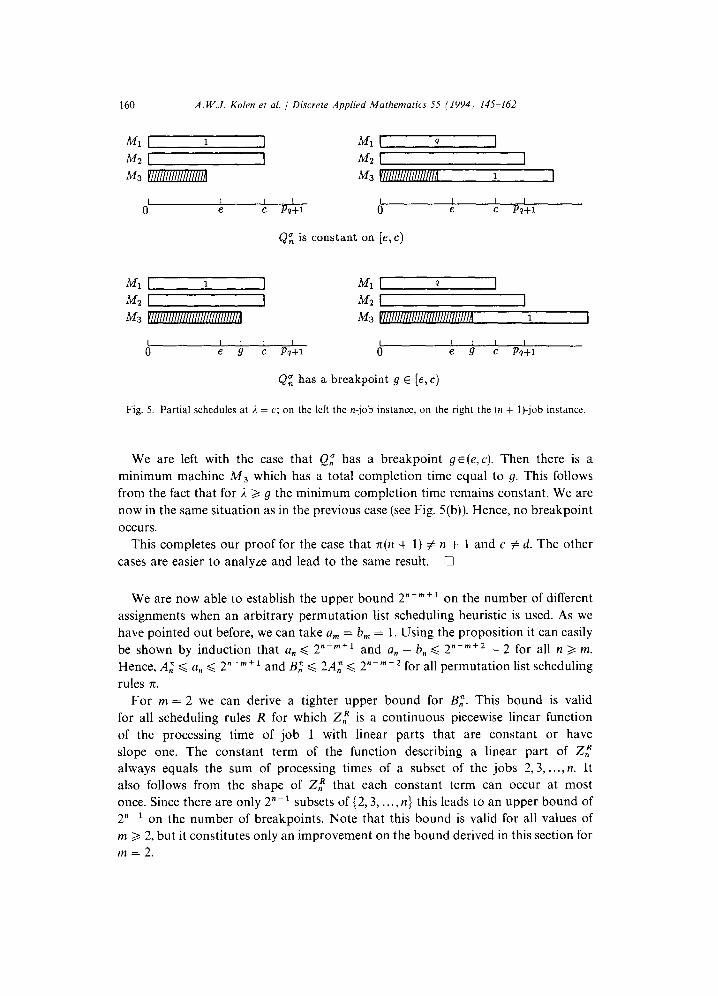
First assume that Ql is constant on [e, c). Consider the n-job instance for ;1 E [e,f).

There is a minimum machine M3 with total processing time less than or equal to e.

This follows from the fact that machine Ml containing only job 1 has a completion

time of e at 13. = e and is increasing as 1” increases. When /1. = c the schedule of the

(n + I)-job instance can be obtained from the schedule of the n-job instance by

replacing job 1 by job q, and placing job 1 on minimum machine M3 (see Fig. 5(a)).

Note that for the (n + 1)-job instance job q has been crashed to c. However, job q + 1

has not been crashed (yet). This explains the difference between the n-job and

(n + I)-job instance with respect to the processing time of the job on MZ. Since Ml (which only contains job q) has a smaller completion time than M3 (which contains

job I), Q;+I is constant on [c,d). Hence, no breakpoint occurs in this interval.

160 A. W.J. Kolen Ed

M3 -

ul. 1 Discrete Applied Mathematics 55 (1994) 145-162

Ml 1 Mz ,,

M3 1 1

I

0 I I I I I I I

e c Pq+l 0 e c Pq+l

Q”, is constant on [e,c)

Ml I I M2 +

MI r I M2 ,b,

M3 M3 1 I

I

0 I I I I

e 9 c Pq+l I

0 I I I I e 9 c P,+1

QE has a breakpoint g E [e,c)

Fig. 5. Partial schedules at i. = c; on the left the n-job instance, on the right the (n + I)-job instance.

We are left with the case that Q; has a breakpoint gE(e, c). Then there is a

minimum machine M3 which has a total completion time equal to g. This follows

from the fact that for ,? 2 g the minimum completion time remains constant. We are

now in the same situation as in the previous case (see Fig. 5(b)). Hence, no breakpoint

occurs.

This completes our proof for the case that n(n + 1) # n + 1 and c # d. The other

cases are easier to analyze and lead to the same result. Cl

We are now able to establish the upper bound 2”-“‘+l on the number of different

assignments when an arbitrary permutation list scheduling heuristic is used. As we

have pointed out before, we can take a, = b, = 1. Using the proposition it can easily

be shown by induction that a, < 2”-m+1 and a,, + b, < 2n-m’2 - 2 for all n > m.

Hence, A,” < a,, < 2”-“‘+’ and B,” d 2A,” < 2n-mf2 for all permutation list scheduling

rules 71.

For m = 2 we can derive a tighter upper bound for B,“. This bound is valid

for all scheduling rules R for which Z,” is a continuous piecewise linear function

of the processing time of job 1 with linear parts that are constant or have

slope one. The constant term of the function describing a linear part of Zf

always equals the sum of processing times of a subset of the jobs 2,3, . . . . n. It

also follows from the shape of Z, R that each constant term can occur at most

once. Since there are only 2”- ’ subsets of {2,3, . . . , n} this leads to an upper bound of

2”-’ on the number of breakpoints. Note that this bound is valid for all values of

m > 2, but it constitutes only an improvement on the bound derived in this section for

m = 2.

A. W.J. K&n et al. / Discrete Applied Mathematics 55 11994) 145-162 161

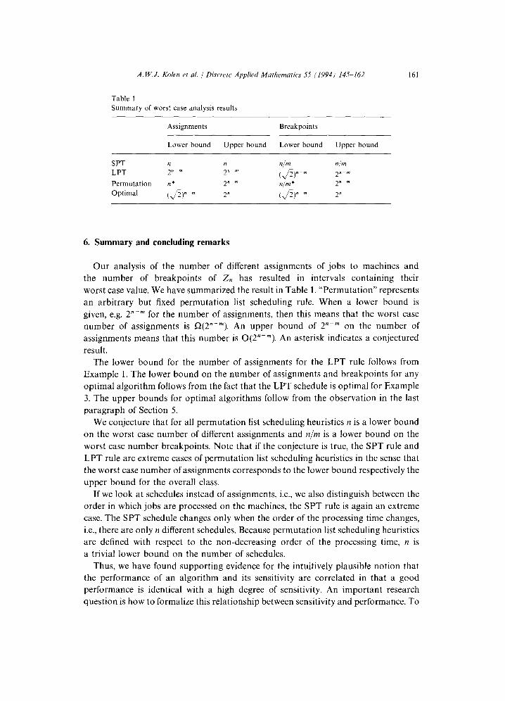
Table 1 Summary of worst case analysis results

Assignments Breakpoints

Lower bound Upper bound Lower bound Upper bound

SPT n

LPT 2”V”

Permutation n*

Optimal CJZY

n nlm nlm 2F” (J5y 2”-” 2°F” n/m * 2”-”

2” CJ;;Y 2”

6. Summary and concluding remarks

Our analysis of the number of different assignments of jobs to machines and

the number of breakpoints of 2, has resulted in intervals containing their

worst case value. We have summarized the result in Table 1. “Permutation” represents

an arbitrary but fixed permutation list scheduling rule. When a lower bound is

given, e.g. 2”-” for the number of assignments, then this means that the worst case

number of assignments is Q(2n-m). An upper bound of 2”-” on the number of

assignments means that this number is O(2”~“‘). An asterisk indicates a conjectured

result.

The lower bound for the number of assignments for the LPT rule follows from

Example 1. The lower bound on the number of assignments and breakpoints for any

optimal algorithm follows from the fact that the LPT schedule is optimal for Example

3. The upper bounds for optimal algorithms follow from the observation in the last

paragraph of Section 5.

We conjecture that for all permutation list scheduling heuristics n is a lower bound

on the worst case number of different assignments and n/m is a lower bound on the

worst case number breakpoints. Note that if the conjecture is true, the SPT rule and

LPT rule are extreme cases of permutation list scheduling heuristics in the sense that

the worst case number of assignments corresponds to the lower bound respectively the

upper bound for the overall class.

If we look at schedules instead of assignments, i.e., we also distinguish between the

order in which jobs are processed on the machines, the SPT rule is again an extreme

case. The SPT schedule changes only when the order of the processing time changes,

i.e., there are only n different schedules. Because permutation list scheduling heuristics

are defined with respect to the non-decreasing order of the processing time, n is

a trivial lower bound on the number of schedules.

Thus, we have found supporting evidence for the intuitively plausible notion that

the performance of an algorithm and its sensitivity are correlated in that a good

performance is identical with a high degree of sensitivity. An important research

question is how to formalize this relationship between sensitivity and performance. To

162 A. W.J. K&n et al. 1 Discrete Applied Mathematics 55 (1994) 145-162

answer this question we need a proper index to measure algorithmic sensitivity. The

functions A,” and B,” used in this paper are a first step in that direction.

Acknowledgements

We would like to thank three anonymous referees for their comments on an earlier

draft of this paper. The third author was supported by the Netherlands Organization

for Scientific Research (NWO) under grant no. 611-304-017. Part of this research was

carried out while the fourth author was visiting the Operations Research Center at the

Massachusetts Institute of Technology with financial support of NWO.

References

[l] J.B.G. Frenk and A.H.G. Rinnooy Kan, The asymptotic optimality of the Ipt rule, Math. Oper. Res. 12 (1987) 241-254.

[Z] R.L. Graham, Bounds for certain multiprocessing anomalies, Bell System Tech. J. 45 (1966) 1563-1581.

[3] R.L. Graham, Bounds on multiprocessing timing anomalies, SIAM J. Appl. Math. 17 (1969) 2633269. [4] E.L. Lawler, J.K. Lenstra, A.H.G. Rinnooy Kan and D.B. Shmoys, Sequencing and scheduling:

algorithms and complexity, in: SC. Graves, A.H.G. Rinnooy Kan and P.H. Zipkin, eds., Logistics of

Production and Inventory, Handbooks in Operations Research and Management Science 4 (North-

Holland, Amsterdam, 1993) Ch. 9, 445-522. [S] A.P.M. Wagelmans, Sensitivity analysis in combinatorial optimization, Ph.D. Thesis, Econometric

Institute, Erasmus University, Rotterdam, Netherlands (1990).