sensitivity analysis of spatial models using ... · pdf fileof spatial models using...

HAL Id: hal-00666755https://hal.archives-ouvertes.fr/hal-00666755

Submitted on 6 Feb 2012

HAL is a multi-disciplinary open accessarchive for the deposit and dissemination of sci-entific research documents, whether they are pub-lished or not. The documents may come fromteaching and research institutions in France orabroad, or from public or private research centers.

L’archive ouverte pluridisciplinaire HAL, estdestinée au dépôt et à la diffusion de documentsscientifiques de niveau recherche, publiés ou non,émanant des établissements d’enseignement et derecherche français ou étrangers, des laboratoirespublics ou privés.

Sensitivity analysis of spatial models using geostatisticalsimulation

Nathalie Saint-Geours, Christian Lavergne, Jean-Stéphane Bailly, FrédéricGrelot

To cite this version:Nathalie Saint-Geours, Christian Lavergne, Jean-Stéphane Bailly, Frédéric Grelot. Sensitivity analysisof spatial models using geostatistical simulation. Robert Marschallinger, Fritz Zobl. MathematicalGeosciences at the Crossroads of Theory and Practice - IAMG 2011 Conference, Sep 2011, Salzburg,Austria. pp.178-189, 2012, <10.5242/iamg.2011.0172>. <hal-00666755>

https://hal.archives-ouvertes.fr/hal-00666755

https://hal.archives-ouvertes.fr

1

Sensitivity analysis of spatial models using geostatistical simulation

Nathalie SAINT-GEOURS1, Christian LAVERGNE2, Jean-Stéphane BAILLY3 & Frédéric GRELOT4

1 AgroParisTech, UMR TETIS, I3M, France, [email protected]

2 I3M, Université Montpellier III, France, [email protected]

3 AgroParisTech, UMR TETIS, France, [email protected] 4 Cemagref, UMR G-EAU, France, [email protected]

Abstract

Geostatistical simulations are used to perform a global sensitivity analysis on a model Y = f(X1 ...

Xk) where one of the model inputs Xi is a continuous 2D-field. Geostatistics allow specifying uncertainty on Xi with a spatial covariance model and generating random realizations of Xi. These random realizations are used to propagate uncertainty through model f and estimate global sensitivity indices. Focusing on variance-based global sensitivity analysis (GSA), we assess in this paper how sensitivity indices vary with covariance parameters (range, sill, nugget). Results give a better understanding on how and when to use geostatistical simulations for sensitivity analysis of spatially distributed models.

1 Introduction

Numerous spatial models are developed to support decision making in various fields of environ-mental management. These models use environmental data that is spatially distributed, including maps derived from sampled data (e.g. digital elevation model, soil map, etc.). These spatial in-puts are always partly uncertain, due to measurement errors, lack of knowledge, aleatory vari-ability (see Refsgaard et al., 2007 for a discussion on the various sources of uncertainty in model inputs). In order to provide confidence in these models, uncertainty analysis (UA) and sensitivity analysis (SA) are increasingly recognized as important steps in the modelling process. They al-low robustness of model predictions to be checked and help identifying the input factors that account for most of model output variability (Saltelli et al., 2008).

Geostatistical simulation has an important role to play in UA/SA of models Y = f(X1 ... Xk) when some model input Xi is a continuous 2D-field. Geostatistics first offers a way to describe the un-certainty on spatial input Xi with a spatial covariance model. Then, random realizations of Xi can be generated through geostatistical simulation (Journel and Huijbregts, 1978). These random realizations can be used to propagate uncertainty through model f and discuss the resulting un-certainty on model output Y (Aerts et al., 2003 - on a problem of optimal location of a ski run; Ruffo et al., 2006 - on hydrocarbon exploration risk evaluation). Within variance-based global sensitivity analysis (GSA) framework, these random realizations can also be sampled alongside with other scalar model inputs to estimate sensitivity indices for each model input (Lilburne & Tarantola, 2009).

Saint-Geours, Lavergne & Bailly

2

Still, a practical problem remains for modellers who intend to use geostatistical simulations in UA/SA of a spatially distributed model: covariance parameters which describe uncertainty on input 2D-field Xi must be estimated carefully, but there is usually few data to support this estima-tion. At the same time, UA/SA results are known to depend heavily on the specification of un-certainty on model inputs. Thus, the following questions arise: to what extent are UA/SA results influenced by spatial covariance parameters? In which cases the uncertainty on input 2D-field Xi accounts for a large or a small part of total variability of model output? To answer these questions, this article aims at determining, in the context of spatial GSA, how sensitivity indices depend on the covariance parameters which describe uncertainty on spatially distributed model inputs. We first describe a simple spatial model Y = f(X, Z) with two inputs: a scalar input X and a 2D spatially distributed input Z(u) (section 2). Then we present variance-based global sensitivity analysis (section 3), and show into details how to estimate sensitivity indices on model M using geostatistical simulations of 2D-field Z(u) (section 4).We finally as-sess the impact of the three usual covariance parameters (range, sill, nugget) on sensitivity indi-ces in model M (section 5). Our results might well prove useful in better understanding the re-sults of a spatial GSA and in deciding whether it is necessary to carefully estimate spatial covari-ance parameters to describe uncertainty on input 2D-fields.

2 A simple spatially distributed model M

For sake of clarity, we will base our paper on a simple case-study. We describe in this section an example of a spatially distributed model M.

4.1 Description of model M

Consider a spatial domain 2RD ⊂ . For numerical application, we represent domain D by a regu-lar square grid G of size 5050 × . We will study in the following sections a model M with two inputs:

( )ZXMY ,=

where:

� ( )21 , XXX = is a vector of two scalars

� Z(u) is a 2D continuous field defined on domain D.

� model output Y(u) is also a 2D continuous field defined by :

( ) ( )( )uZXfuYDu ,, =∈∀

Function f(.,.) can be any mapping from ℝ3 to ℝ. For numerical application, we arbitrarily choose

the following mapping:

( ) ( ))(4010,, )(036.02

21

321 uZexxzxxf uZ ⋅+⋅+⋅= ⋅−

Model M is a “point-based model”: the value of model output Y(u) at any point Du ∈ only de-

pends on the scalar inputs ( )21, XX and on the value of Z(u) at the same point u. Point-based

models are encountered in many environmental applications. For example, M could be a spatially distributed model used for economic assessment of flood risk: in this case, model input Z(u) could be a map of the maximal water levels reached during a flood event over a given area D,

Using geostatistical simulations for sensitivity analysis of spatially distributed models

3

( )21 , XXX = would be a set of economic parameters, and model output Y(u) would be the map

of expected damages due to the flood over the area.

4.2 Output of interest

In order to perform sensitivity analysis of model M, we need to consider a single scalar quantity of interest derived from model output Y(u). In most applications, the output of interest is either the value of 2D-field Y(u) at some specific point u of the study area, or the mean (or total) value

of Y(u) over a given zone within the study area. Here we define the output of interest DY as the

mean value of field Y(u) over spatial domain D:

( )∫∈

⋅⋅=Du

D duuYD

Y1

In the following sections we will use variance-based global sensitivity analysis to assess the vari-

ability of DY due to the uncertainty on model inputs X and Z(u).

3 Variance-based global sensitivity analysis

Sensitivity analysis (SA) aims at a studying how uncertainty in the output of a model can be apportioned to different sources of uncertainty in the model inputs. Among the various available SA techniques (see Helton and Davis, 2006 for a review), variance-based global sensitivity analysis (GSA) has several advantages: it explores widely the space of uncertain input factors and is suitable for complex models with non-linear effects and interactions among factors. GSA is based on the decomposition of the variance of model output Y in conditional variances. It leads to the definition of two importance measures for each input factor Xi of a model: first-order sensitivity index Si and total-order sensitivity index STi. First-order sensitivity index of input factor Xi is defined by:

[ ]( )( )YVar

XYEVarS

i

i =

Si measures the main effect contribution of input factor Xi to the variance of model output Y. It is the expected part of output variance Var(Y) that could be reduced if input factor Xi was perfectly known. Total order sensitivity index STi of input factor Xi is defined as:

[ ]( )( )YVar

XYVarEST

i

i

~=

where X~i denotes all input factors but Xi. STi measures the contribution of input factor Xi and all its interactions with other input factors Xj to the variance of model output Y. It is the expected part of output variance Var(Y) that would remain if all input factors but Xi were perfectly known. Sensitivity indices can be used to identify the model inputs that account for most of model output variability (input factors Xi with high first order indices Si); it may lead to model simplification by identifying model inputs that have little influence on model output variance (input factors Xi with low total order sensitivity indices STi); it also allows discussing the contribution of interactions between input factors to the model output variance (comparison between first and total order sensitivity indices). For more details on GSA basics, see Saltelli et al., 2008.


4

4 Estimating sensitivity indices using geostatistical simulations

GSA was initially designed to study models with scalar inputs only. Some authors have sug-gested solutions to handle spatially distributed inputs as well (Volkova et al., 2008 ; Iooss & Ri-batet, 2009; Ruffo et al., 2006; Lilburne & Tarantola, 2009). We describe in this section how to estimate sensitivity indices in model M by associating randomly generated realizations of uncer-tain 2D-field Z(u) to scalar values, according to the approach developed by Lilburne and Taran-tola.

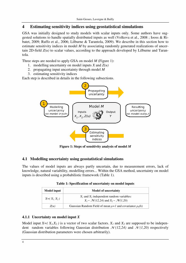
Three steps are needed to apply GSA on model M (Figure 1): 1. modelling uncertainty on model inputs X and Z(u) 2. propagating input uncertainty through model M 3. estimating sensitivity indices

Each step is described in details in the following subsections.

Figure 1: Steps of sensitivity analysis of model M

4.1 Modelling uncertainty using geostatistical simulations

The values of model inputs are always partly uncertain, due to measurement errors, lack of knowledge, natural variability, modelling errors... Within the GSA method, uncertainty on model inputs is described using a probabilistic framework (Table 1).

Table 1: Specification of uncertainty on model inputs

Model input Model of uncertainty

X=( X1, X2 ) X1 and X2 independent random variables:

X1 ~ N (12,24) and X2 ~ N (1,20)

Z(u) Gaussian Random Field of mean µ=1 and covariance ρθ(h)

4.1.1 Uncertainty on model input X

Model input X=( X1,X2 ) is a vector of two scalar factors. X1 and X2 are supposed to be indepen-dent random variables following Gaussian distribution N (12,24) and N (1,20) respectively (Gaussian distribution parameters were chosen arbitrarily).


5

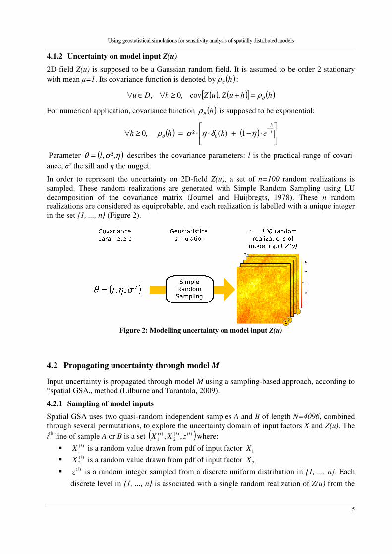
4.1.2 Uncertainty on model input Z(u)

2D-field Z(u) is supposed to be a Gaussian random field. It is assumed to be order 2 stationary

with mean µ=1. Its covariance function is denoted by ( )hθρ :

( ) ( )[ ] ( )hhuZuZhDu θρ=+≥∀∈∀ ,cov,0,

For numerical application, covariance function ( )hθρ is supposed to be exponential:

( ) ( )

⋅−+⋅⋅=≥∀

−l

h

ehhh ηδησρθ 1)(²,0 0

Parameter ( )ησθ ²,,l= describes the covariance parameters: l is the practical range of covari-

ance, σ² the sill and η the nugget.

In order to represent the uncertainty on 2D-field Z(u), a set of n=100 random realizations is sampled. These random realizations are generated with Simple Random Sampling using LU decomposition of the covariance matrix (Journel and Huijbregts, 1978). These n random realizations are considered as equiprobable, and each realization is labelled with a unique integer in the set {1, ..., n} (Figure 2).

Figure 2: Modelling uncertainty on model input Z(u)

4.2 Propagating uncertainty through model M

Input uncertainty is propagated through model M using a sampling-based approach, according to “spatial GSA„ method (Lilburne and Tarantola, 2009).

4.2.1 Sampling of model inputs

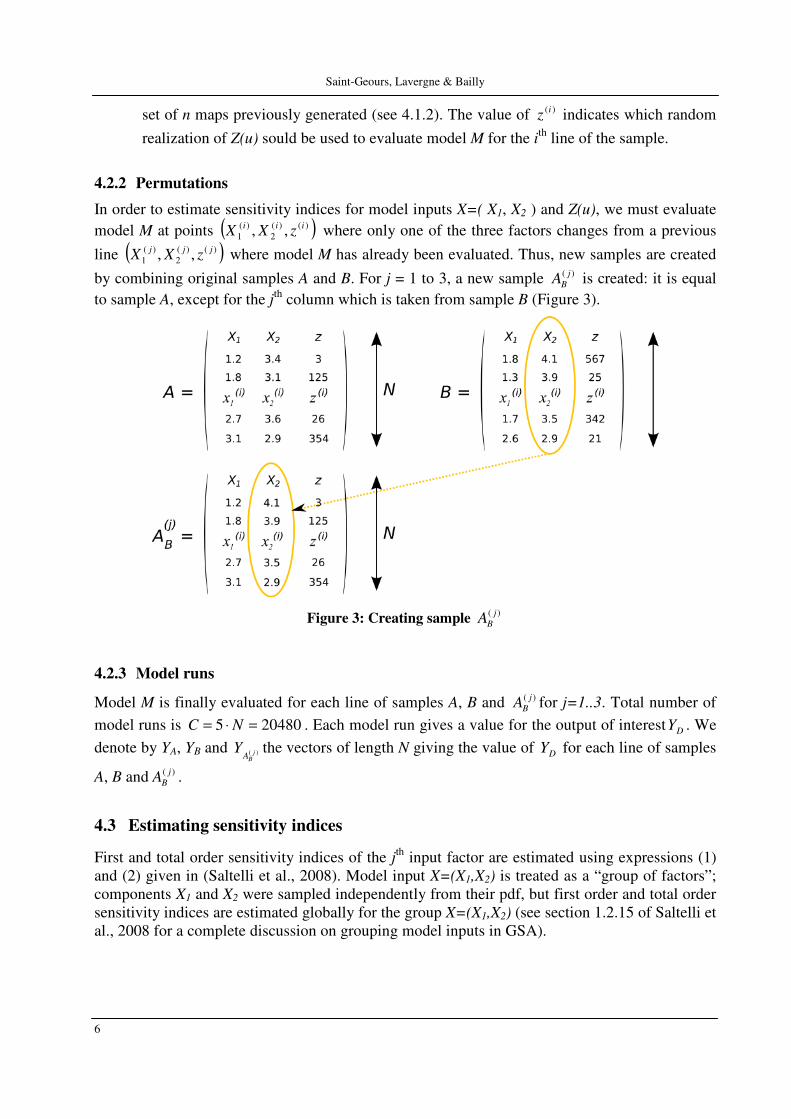
Spatial GSA uses two quasi-random independent samples A and B of length N=4096, combined through several permutations, to explore the uncertainty domain of input factors X and Z(u). The

ith line of sample A or B is a set ( ))()(

2)(

1 ,, iii zXX where:

� )(1

iX is a random value drawn from pdf of input factor 1X

� )(2

iX is a random value drawn from pdf of input factor 2X

� )(iz is a random integer sampled from a discrete uniform distribution in {1, ..., n}. Each

discrete level in {1, ..., n} is associated with a single random realization of Z(u) from the


6

set of n maps previously generated (see 4.1.2). The value of )(iz indicates which random

realization of Z(u) sould be used to evaluate model M for the ith line of the sample.

4.2.2 Permutations

In order to estimate sensitivity indices for model inputs X=( X1, X2 ) and Z(u), we must evaluate

model M at points ( ))()(2

)(1 ,, iii zXX where only one of the three factors changes from a previous

line ( ))()(2

)(1 ,, jjj zXX where model M has already been evaluated. Thus, new samples are created

by combining original samples A and B. For j = 1 to 3, a new sample )( j

BA is created: it is equal

to sample A, except for the jth column which is taken from sample B (Figure 3).

Figure 3: Creating sample )( j

BA

4.2.3 Model runs

Model M is finally evaluated for each line of samples A, B and )( j

BA for j=1..3. Total number of

model runs is 204805 =⋅= NC . Each model run gives a value for the output of interest DY . We

denote by YA, YB and )( jBA

Y the vectors of length N giving the value of DY for each line of samples

A, B and )( j

BA .

4.3 Estimating sensitivity indices

First and total order sensitivity indices of the jth input factor are estimated using expressions (1) and (2) given in (Saltelli et al., 2008). Model input X=(X1,X2) is treated as a “group of factors”; components X1 and X2 were sampled independently from their pdf, but first order and total order sensitivity indices are estimated globally for the group X=(X1,X2) (see section 1.2.15 of Saltelli et al., 2008 for a complete discussion on grouping model inputs in GSA).


7

⋅⋅

⋅−⋅⋅

⋅⋅−⋅⋅

=

∑∑∑

∑∑

===

==

N

i

i

B

N

i

i

A

N

i

i

A

i

A

N

i

i

A

i

B

N

i

i

A

i

B

j

YN

YN

YYN

YYN

YYN

S

jB

1

)(

1

)(

1

)()(

1

)()(

1

)()(

111

11)(

(1)

( )

⋅⋅

⋅−⋅⋅

−⋅

=

∑∑∑

∑

===

=

N

i

i

B

N

i

i

A

N

i

i

A

i

A

N

i

i

A

i

A

j

YN

YN

YYN

YYN

ST

jB

1

)(

1

)(

1

)()(

1

2)()(

111

2

1)(

(2)

We finally obtain four different sensitivity indices: first and total order sensitivity indices of model input X=( X1,X2 ), denoted by SX and STX ; first and total order sensitivity indices of model input Z(u), denoted by SZ and STZ. In the current case of a model with only two inputs (X and Z(u)), the following properties hold:

STX = SX + SX,Z and STZ = SZ + SX,Z

where SX,Z = 1 - SX - SZ is a second order sensitivity index which accounts for the contribution of the interaction between X and Z(u) to the variance of model output YD. Thus, we will only pay attention in the following sections to first order indices SX and SZ.

5 Influence of covariance parameters on sensitivity indices

In this section, we want to assess how GSA results on model M are influenced by covariance

parameters ( )ησ ²,,l . 26 different sets ( )kkkk l ησθ ²,,= of covariance range, sill and nugget are

defined (Table 2). For each set kθ of covariance parameters, GSA is performed as follows:

� a set of n=100 random realizations of input random field Z(u) is generated using geosta-tistical simulation as described in 4.1

� uncertainty is propagated through model M as described in 4.2

� total variance of model output YD is computed

� first order sensitivity indices SX and SZ are estimated as described in 4.3.

The whole procedure is replicated 100 times. Then, for each set of covariance parameters, mean value of Var(YD), SX and SZ and their 95% confidence interval over the 100 replicas are compu-ted.

Table 2: Sets of covariance parameters

Covariance parameters Set name

Range l Sill σ² (square root) Nugget η

θ1 to θ8 5 to 40 (step 5) 70 0.1

θ9 to θ16 60 20 to 55 (step 5) 0.1

θ17 to θ26 60 70 0.1 to 1 (step 0.1)


8

5.1 Influence of the ratio covariance range l / size of domain D

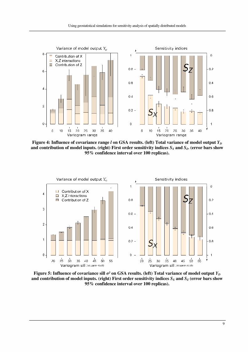
Fig 4. shows output variance Var(YD) and sensitivity indices SX and SZ for increasing covariance range l (sets θ1 to θ8). It appears that the absolute contribution of model input Z(u) to total output variance Var(YD) increases with covariance range l, while absolute contribution of model input X remains constant. Accordingly, sensitivity index of model input Z(u) increases with covariance range l, while sensitivity index of X decreases when covariance range l increases.

Let define the ratio r of covariance range l compared to the size of domain D: Dlr /= . This

numerical case-study illustrates the following property: the larger the ratio r, the larger the part of output variance Var(YD) explained by the uncertainty on Z(u). For a low ratio (i.e. when range l is small compared to the size of domain D), variability of Z(u) is mainly “local”, and spatial correlation of Z(u) variability over domain D is weak. This “local” variability averages over domain D when model output YD is computed. Thus the uncertainty on input 2D-field Z(u) has a small influence on output variance Var(YD). On the contrary, for a greater ratio r (i.e. when range l is large compared to the size of domain D), spatial correlation of Z(u) variability over domain D is strong. The averaging effect of “local” variability of Z(u) over domain D is weaker. Thus the uncertainty on input 2D-field Z(u) has a larger influence on output variance Var(YD).

5.2 Influence of covariance sill

Fig 5. shows output variance Var(YD) and sensitivity indices SX and SZ for increasing covariance sill σ² (sets θ9 to θ16). It appears that the absolute contribution of model input Z(u) to total output variance Var(YD) increases with covariance sill σ², while absolute contribution of model input X remains constant. Accordingly, sensitivity index of model input Z(u) increases with covariance sill σ², while sensitivity index of X decreases when covariance sill σ² increases. This numerical case-study illustrates the following straightforward property: the larger the covariance sill σ² in random field Z(u), the larger the part of output variance Var(YD) explained by the uncertainty on Z(u). Covariance sill σ² controls the overall variability of model input Z(u), thus sensitivity index of Z(u) with respect to model output YD is a monotonically increasing function of sill σ².

5.3 Influence of covariance nugget

Fig 6. shows output variance Var(YD) and sensitivity indices SX and SZ for increasing covariance nugget h (sets θ17 to θ26). It appears that the absolute contribution of model input Z(u) to total output variance Var(YD) decreases when covariance nugget h increases, while absolute contribution of model input X remains constant. Accordingly, sensitivity index of model input Z(u) decreases when covariance nugget h increases. Nugget parameter h controls the intensity of “noise” in Gaussian random field Z(u). When h is close to 1, the largest part of Z(u) variability is due to the “nugget effect”, i.e. to “local” noise at each point Du ∈ with no spatial correlation. This local noise averages over domain D when model output YD is computed. Thus the uncertainty on input 2D-field Z(u) has a small influence on output variance Var(YD). On the contrary, for a lower value of nugget parameter, (h close to 0), most of the uncertainty in random field Z(u) is spatially correlated, and local noise plays a small part. The averaging effect of uncorrelated variability of Z(u) over domain D is weaker. Thus the uncertainty on input 2D-field Z(u) has a larger influence on output variance Var(YD).


9

Figure 4: Influence of covariance range l on GSA results. (left) Total variance of model output YD

and contribution of model inputs. (right) First order sensitivity indices SX and SZ. (error bars show

95% confidence interval over 100 replicas).

Figure 5: Influence of covariance sill σ² on GSA results. (left) Total variance of model output YD

and contribution of model inputs. (right) First order sensitivity indices SX and SZ (error bars show



10

Figure 6: Influence of covariance nugget η on GSA results. (left) Total variance of model output YD

and contribution of model inputs. (right) First order sensitivity indices SX and SZ (error bars show


6 Discussion

This research sought to illustrate on a simple case-study how to use geostatistical simulation to perform variance-based global sensitivity analysis (GSA) on a spatially distributed model. We also aimed at exploring how GSA results depend on covariance parameters chosen to describe uncertainty on spatially distributed model inputs.

6.1 Using geostatistical simulation for spatial GSA

We demonstrated on a simple case-study the suitability of “spatial GSA” approach (Lilburne & Tarantola, 2009) to perform sensitivity analysis on a spatially distributed model with continuous 2D-fields inputs. Geostatistical simulation was used to generate a set of n random realizations of continuous 2D-field Z(u) and estimate sensitivity indices of uncertain model inputs Z(u) and X through a sampling-based approach. Spatial GSA makes it possible to account for the relative contribution of each uncertain model input to the total variance of model output. It helps assess-ing model robustness and should be systematically performed when developing a model with uncertain spatial inputs. Nevertheless, two limits of this approach must be highlighted:

� spatial GSA is a sampling-based approach which needs lots of model runs to estimate sensitivity indices. As a consequence, it is limited to models with low CPU-cost. For high CPU-cost models, other sensitivity analysis methods such as Elementary Effects or One-At-a-Time should be applied (see Saltelli et al., 2008).

� spatial GSA uses a set of n random realizations to represent the uncertainty on spatial in-put Z(u) (assumed to be a Gaussian Random Field). When n is too low, the small set of map simulations fails to capture the overall variability of Z(u), and sensitivity indices estimates SX and SZ are biased. Previous work had been carried out to compare the use of two different geostatistical simulation algorithms (Simple Random Sampling and Latin Hypercube Sampling) to generate realizations of spatial input Z(u) for GSA (Kyriakydis, 2005; Saint-Geours et al., 2010), but no optimal sampling strategy was found to reduce this bias.


11

6.2 Impact of spatial covariance parameters on spatial GSA

The influence of covariance range, sill and nugget on sensitivity indices was assessed on a sim-ple case-study. It was initially suggested that covariance parameters chosen to describe uncer-tainty on spatial input Z(u) would influence GSA results. Our results prove such to be the case. On our case-study, it appears that first order sensitivity index SZ of model input Z(u) is a monoti-cally increasing function of both covariance range l and covariance sill σ², and a decreasing func-tion of covariance nugget η.

These properties were only illustrated on a simple case-study with a specific model M and an exponential covariance function. Nevertheless, it can be analytically shown (on-going work) that these properties are actually verified for any monotically increasing covariance function and for any point-based model M where mapping f is square-integrable.

Results of this study may well help modellers when estimating spatial covariance parameters to describe uncertainty on a spatial input Z(u) for sensitivity analysis of a spatially distributed model. When field data is lacking to carefully estimate covariance parameters, at least the a-

priori impact of giving wrong values to these parameters will be known: over-estimating covari-ance range l or covariance sill σ² wil result in over-estimating sensitivity indices of spatial input Z(u) and under-estimating sensitivity indices of scalar inputs Xi. On the contrary, over-estimating covariance nugget η will result in under-estimating sensitivity indices of Z(u).

7 Conclusion

Variance-based global sensitivity analysis (GSA) was performed on a simple example of a spa-tially distributed model Y=M(X,Z) with two inputs: a scalar input X and a spatial input Z(u). In order to represent the variability on uncertain spatial input Z(u), it was assumed to be a Gaussian Random Field, and random realizations were generated using geostatistical simulation. These random realizations were used to propagate input uncertainty through model M. Sensitivity indi-ces of model inputs X and Z(u) were estimated with a sampling-based approach. The influence of spatial covariance parameters on GSA results was assessed by estimating sensitivity indices for different sets of covariance range, sill and nugget.

Results show that (1) first order sensitivity index SZ of spatial input Z(u) is a monotically increas-ing function of covariance range l (2) first order sensitivity index SZ of spatial input Z(u) is a monotically increasing function of covariance sill σ² (3) first order sensitivity index SZ of spatial input Z(u) is a monotically decreasing function of covariance nugget η.

These empirical results may be of importance when setting covariance parameters to describe uncertainty in spatial inputs for sensitivity analysis of a spatial model. Yet further research is needed to prove analytically that these properties hold for a large range of point-based models and monotonic covariance functions. Such study may help promoting the use of geostatistical simulation to perform sensitivity analysis of spatially distributed models.


12

References

AERTS, J. C. J. H., HEUVELINK, G. B. M., GOODCHILD, M. F. (2003): Accounting for spatial uncertainty in optimization with spatial decision support systems. Transactions in GIS, Vol. 7, 211-230

HELTON, J. C., DAVIS, F. J. (2006): Sampling-based methods for uncertainty and sensitivity analysis. Multimedia Environmental Models, Vol. 32, 135-154

IOOSS, B., RIBATET, M. (2009): Global sensitivity analysis of computer models with func-tional inputs. Reliability Engineering and System Safety, Vol. 94, 1194 - 1204

JOURNEL, A.G., HUIJBREGTS, C.J. (1978): Mining geostatistics. The Blackburn Press

KYRIAKIDIS, P. C. (2005): Sequential spatial simulation using Latin Hypercube Sampling. Geostatistics Banff 2004, 65-74

LILBURNE, L., TARANTOLA, S. (2009): Sensitivity analysis of spatial models. Interna-tional Journal of Geographical Information Science, Vol. 23, No. 2, 151-168

REFSGAARD, J. C., VAN DER SLUIJS, J. P., HØJBERG, A. L., VANROLLEGHEM, P. A. (2007): Uncertainty in the environmental modelling process: a framework and guidance. Envi-ronmental Modelling and Software, Vol. 22, 1543-1556

RUFFO, P., BAZZANA, L., CONSONNI, A., CORRADI, A., SALTELLI, A., TARANTO-LA, S. (2006): Hydrocarbon exploration risk evaluation through uncertainty and sensitivity analyses techniques. Reliability Engineering and System Safety, Vol. 91, 1155-1162

SAINT-GEOURS, N., BAILLY, J.-S., GRELOT, F., LAVERGNE, C. (2010): Is there room to optimise the use of geostatistical simulations for sensitivity analysis of spatially distributed models ? Accuracy 2010 : proceedings of the ninth International Symposium on Spatial Accu-racy Assesment in Natural Resources and Environmental Sciences, 81-84

SALTELLI, A., RATTO, M., ANDRES, T., CAMPOLONGO, F., CARIBONI, J., GATELLI, D., SAISANA, M., TARANTOLA, S. (2008): Global Sensitivity Analysis - The Primer. Wiley, New-York.

VOLKOVA, E., IOOSS, B., VAN DORPE, F. (2008): Global sensitivity analysis for a nu-merical model of radionuclide migration from the RRC Kurchatov Institute radwaste disposal site. Stochastic Environmental Research and Risk Assessment, Vol. 22, 17-31

sensitivity analysis of spatial models using ... · pdf fileof spatial models using...

Documents