sensor fusion for mechatronic systems - unipd.itpaduaresearch.cab.unipd.it/2817/1/phdthesis.pdf ·...
TRANSCRIPT
Methods and applications of “sensor fusion” for
mechatronic systems
Metodi e applicazioni di sensor fusion per sistemimeccatronici
Francesco Setti
January 28, 2010

ii

To Stefania
iii

iv

Acknowledgments
It is with great pleasure that I am here, once again, to thank those who madethis possible. First I want to thank my advisor, prof. Mariolino De Cecco;already three years ago he believed in me, he gave me the opportunity toreach this new goal and has always guaranteed its support.
For the same support I must also be grateful to all my colleagues in theMeasurement Group and, more generally, in the Mechatronics Group at theUniversity of Trento; to list all them would take too long, thanks collectively!
This work was partially supported by Delta R&S, thanks to them, whichI hope does not end there.
Many thanks to Alessio Del Bue and all the “Lisboetas” for three intensemonths of work, but not only...
I owe a special thanks to those who accompanied me in these years:Matteo and Bicio. Like three years ago, we are, this time away, to celebratea new degree.
I would also like to thank my parents Silvano and Patrizia, my sisterChiara, Robby and all my relatives for the support they provided me throughmy entire life and in particular in these last three years.
I can not forget Marco, Elena and Andrea who are now part of my family.I must acknowledge my best friends Matteo, Elena, Fabio, Anna, Roberto
and Veronica simply for being with me.
However, remember that the greatest acknowledgment is not a thanksbut a dedication!
v

vi

Abstract
In this paper we present a system for 3D shapes digitization. During the re-search we developed algorithms for 3D shapes reconstruction from multiplestereo images; this algorithms provide the use of colored markers lying overthe object surface. The procedure developed provides steps of image pro-cessing for markers detection, 3D reconstruction based on epipolar geometryand data fusion from different stereo-pairs. Particular attention was paid tothe latter point, developing an algorithm based on uncertainty analysis ofeach 3D point and compatibility analysis by the Mahalanobis distance. Werethen developed algorithms for modeling 3D objects in the scene based on aimages sequence of moving bodies. A physical prototype was created at theMeccaLab at University of Trento and it has been used for an experimentalverification of the proposed algorithms.
Sommario
In questo lavoro viene presentato un sistema di digitalizzazione di forme3D. Nel corso della ricerca sono stati sviluppati degli algoritmi per la ri-costruzione di forme 3D a partire da immagini acquisite da piu stereo-camere; questi algoritmi prevedono l’utilizzo di marker colorati posizionatisull’oggetto da digitalizzare. La procedura sviluppata prevede fasi di elabo-razione delle immagini per la localizzazione dei marker, ricostruzione 3Dbasata sulla geometria epipolare e fusione dei dati provenienti dalle di-verse stereocamere. Particolare attenzione e stata posta a quest’ultimopunto, sviluppando un algoritmo basato su analisi dell’incertezza di ognipunto e analisi di compatibilita dei punti mediante distanza di Mahalanobis.Vengono poi proesentati degli algoritmi per la modellazione degli oggetti3D presenti nella scena sulla base di una sequenza di immagini dei corpiin movimento. Un prototipo fisico e stato realizzato presso il MeccaLabdell’Universita di Trento ed e stato utilizzato per una fase sperimentale diverifica degli algoritmi proposti.
vii

viii
Contents
1 Introduction 1
I Introduction to computer vision 7
2 Camera model 9
2.1 What’s an image? . . . . . . . . . . . . . . . . . . . . . . . . 9
2.2 The thin lens model . . . . . . . . . . . . . . . . . . . . . . . 10
2.3 The pinhole model . . . . . . . . . . . . . . . . . . . . . . . . 11
2.4 Reference frames and conventions . . . . . . . . . . . . . . . . 12
2.5 Geometric model of projection . . . . . . . . . . . . . . . . . 13
2.6 Camera parameters . . . . . . . . . . . . . . . . . . . . . . . . 14
2.6.1 Intrinsic parameters . . . . . . . . . . . . . . . . . . . 14
2.6.2 Extrinsic parameters . . . . . . . . . . . . . . . . . . . 15
2.6.3 Distortion . . . . . . . . . . . . . . . . . . . . . . . . . 15
3 Geometry of two cameras 17
3.1 Epipolar geometry . . . . . . . . . . . . . . . . . . . . . . . . 17
3.2 Stereo camera model . . . . . . . . . . . . . . . . . . . . . . . 18
3.3 Triangulation . . . . . . . . . . . . . . . . . . . . . . . . . . . 19
3.3.1 Ideal case . . . . . . . . . . . . . . . . . . . . . . . . . 19
3.3.2 Real case . . . . . . . . . . . . . . . . . . . . . . . . . 20
II Proposed algorithms 23
4 Algorithm for static reconstruction 25
4.1 Feature extraction . . . . . . . . . . . . . . . . . . . . . . . . 26
4.1.1 Feature detection . . . . . . . . . . . . . . . . . . . . . 26
4.1.2 Feature description . . . . . . . . . . . . . . . . . . . . 28
4.2 Stereo-reconstruction . . . . . . . . . . . . . . . . . . . . . . . 29
4.2.1 Finding the starting stripe . . . . . . . . . . . . . . . . 30
4.2.2 Expansion from starting stripe . . . . . . . . . . . . . 30
4.3 Points fusion . . . . . . . . . . . . . . . . . . . . . . . . . . . 31
ix
x CONTENTS
4.3.1 Uncertainty analysis . . . . . . . . . . . . . . . . . . . 314.3.2 Uncertainty propagation . . . . . . . . . . . . . . . . . 34
4.4 Compatibility analysis . . . . . . . . . . . . . . . . . . . . . . 36
5 Algorithm for Motion Capture 395.1 Image acquisition and 3D reconstruction . . . . . . . . . . . . 395.2 Trajectory matrix . . . . . . . . . . . . . . . . . . . . . . . . . 41
5.2.1 Matching using Nearest Neighbor . . . . . . . . . . . . 425.2.2 Matching using NN and Procrustes analysis . . . . . . 43
5.3 Motion Segmentation . . . . . . . . . . . . . . . . . . . . . . . 455.3.1 GPCA algorithm . . . . . . . . . . . . . . . . . . . . . 455.3.2 RANSAC algorithm . . . . . . . . . . . . . . . . . . . 465.3.3 LSA algorithm . . . . . . . . . . . . . . . . . . . . . . 47
5.4 Joint Reconstruction . . . . . . . . . . . . . . . . . . . . . . . 545.4.1 Factorization method . . . . . . . . . . . . . . . . . . 54
III Experimental section 61
6 Experimental section 636.1 Experimental setup . . . . . . . . . . . . . . . . . . . . . . . . 636.2 Experiments of static reconstruction . . . . . . . . . . . . . . 65
6.2.1 Single stereo-pair verification . . . . . . . . . . . . . . 656.2.2 Data fusion verification . . . . . . . . . . . . . . . . . 66
6.3 Experiments of motion capture . . . . . . . . . . . . . . . . . 686.3.1 Rigid bodies . . . . . . . . . . . . . . . . . . . . . . . 696.3.2 Deformable bodies . . . . . . . . . . . . . . . . . . . . 70
7 Conclusions 73
List of Figures
2.1 Graphic representation of the thin lens model. . . . . . . . . . 10
2.2 Graphic representation of the pinhole model. . . . . . . . . . . 11
2.3 Graphic representation of the frontal pinhole model. . . . . . 12
2.4 The ideal pinhole camera model with all the reference framesused in this work. . . . . . . . . . . . . . . . . . . . . . . . . . 13
3.1 The epipolar geometry representation. . . . . . . . . . . . . . 18
3.2 The triangulation geometry in an ideal case. . . . . . . . . . . 19
3.3 The triangulation geometry in an real case. . . . . . . . . . . 20
4.1 Static reconstruction algorithm functional description . . . . 26
4.2 The image segmentation process. . . . . . . . . . . . . . . . . 28
4.3 Example of badly segmented elliptical marker. . . . . . . . . . 34
4.4 An example of different Mahalanobis Distance between thesame couple of points. . . . . . . . . . . . . . . . . . . . . . . 37
4.5 An example of covariance ellipsoid of a fused point. . . . . . . 38
5.1 The flow chart of our approach to the motion capture problem. 40
5.2 An example of a set of images acquired from the stereo-pairs. 40
5.3 The pattern used for the 3d reconstruction. . . . . . . . . . . 40
5.4 An example of a set of frames used for the motion segmenta-tion and joint reconstruction. . . . . . . . . . . . . . . . . . . 41
5.5 A graphical explanation of the Procrustes Analysis applied tothe point matching. . . . . . . . . . . . . . . . . . . . . . . . . 44
5.6 An example of trajectory of points in a sequence of eight frames. 44
5.7 The expected critical zone in motion segmentation. . . . . . . 46
5.8 An example of motion segmentation using the GeneralizedPrincipal Component Analysis (GPCA). . . . . . . . . . . . . 47
5.9 An example of motion segmentation using the RANSAC. . . 47
5.10 Example of trajectories that belong to two different subspacesof dimension 2 projected into an R3 unit sphere. . . . . . . . 49
5.11 Example of affinity matrix of the trajectories of three clusters. 50
5.12 Example of affinity matrix rearranged after the spectral clus-tering. This is the same affinity matrix shown in Figure 5.11. 52
xi
xii LIST OF FIGURES
5.13 Local Subspace Affinity workflow. . . . . . . . . . . . . . . . . 535.14 An example of motion segmentation using the Local Subspace
Affinity (LSA). . . . . . . . . . . . . . . . . . . . . . . . . . . 535.15 An example of joint estimation using the Fayad’s algorithm. . 60
6.1 The experimental setup . . . . . . . . . . . . . . . . . . . . . 636.2 The angle between cameras in a stereo-pair. . . . . . . . . . . 646.3 The acquired images in the inclined plane experiment. . . . . 656.4 The 3D reconstruction of the inclined plane experiment. . . . 666.5 The acquired images in the inclined plane experiment. . . . . 666.6 The inclined-can experimental setup. . . . . . . . . . . . . . . 676.7 The markers on the can reconstructed from 2 stereo-pairs. . . 676.8 Covariance elliposids of two corresponding points (obtained
from the same marker) acquired by two stereo-pairs. . . . . . 686.9 Covariance ellipsoids of all the markers in position A. . . . . 686.10 Blue vectors shown the estimated displacements of matching
points of A (green markers) and B (red markers). . . . . . . . 696.11 The first experiment: two rigid bodies with axial joint. . . . . 696.12 The second experiment: a real human arm. . . . . . . . . . . 70
Chapter 1
Introduction
A 3D scanner is a device that analyzes a real-world object or environmentto collect data on its shape and, if interesting, its appearance (e.g. color).The collected data can then be used to construct digital, three dimensionalmodels useful for a wide variety of applications. These devices are usedextensively by the entertainment industry, in the production of movies andvideo games, but also in industrial design, orthotics and prosthetics, reverseengineering and prototyping, quality control/inspection and documentationof cultural artifacts.
The purpose of a 3D scanner is usually to create a point cloud of geo-metric samples on the surface of the subject. These points can then be usedto extrapolate the shape of the subject. Many different technologies can beused to build these 3D scanning devices; each technology comes with its ownlimitations, advantages and costs.
For most situations, a single scan will not produce a complete model ofthe subject. Multiple scans, even hundreds, from many different directionsare usually required to obtain information about all sides of the subject.These scans have to be brought in a common reference frame, a processthat is usually called alignment or registration, and then merged to createa complete model.
There are two types of 3D scanners: contact and non-contact. Non-contact 3D scanners can be further divided into two main categories, activescanners and passive scanners. There are a variety of technologies that fallunder each of these categories.
Contact 3D scanners probe the subject through physical touch. A Coor-dinate Measuring Machine (CMM)(Spitz, 1999) is an example of a contact3D scanner. It is used mostly in manufacturing and can be very precise.The disadvantage of CMMs though, is that it requires contact with the ob-ject being scanned. Thus, the act of scanning the object might modify or
1
2 CHAPTER 1. INTRODUCTION
damage it. This fact is very significant when scanning delicate or valuableobjects such as historical artifacts. The other disadvantage of CMMs is thatthey are relatively slow compared to the other scanning methods. Physi-cally moving the arm that the probe is mounted on can be very slow andthe fastest CMMs can only operate on a few hundred hertz.
Non-contact active scanners emit some kind of radiation or light anddetect its reflection in order to probe an object or environment. Possibletypes of emissions used include light, ultrasound or x-ray. Some examplesof non-contact active devices are time-of-flight laser scanner, triangulationlaser scanner and structured light.
The time-of-flight 3D laser scanner is an active scanner that uses laserlight to probe the subject. At the heart of this type of scanner is a time-of-flight laser rangefinder. The laser rangefinder finds the distance of a surfaceby timing the round-trip time of a pulse of light. A laser is used to emita pulse of light and the amount of time before the reflected light is seenby a detector is timed. Since the speed of light c is known, the round-trip time determines the travel distance of the light, which is twice thedistance between the scanner and the surface. The accuracy of a time-of-flight 3D laser scanner depends on how precisely we can measure the time.The laser rangefinder only detects the distance of one point in its direction ofview. Thus, the scanner scans its entire field of view one point at a time bychanging the range finder’s direction of view to scan different points. Theview direction of the laser rangefinder can be changed by either rotatingthe range finder itself, or by using a system of rotating mirrors. The lattermethod is commonly used because mirrors are much lighter and can thusbe rotated much faster and with greater accuracy. Typical time-of-flight 3Dlaser scanners can measure the distance of 10.000 ÷ 100.000 points everysecond.
The triangulation 3D laser scanner is also an active scanner that useslaser light to probe the environment. With respect to time-of-flight 3D laserscanner the triangulation laser shines a laser on the subject and exploitsa camera to look for the location of the laser dot. Depending on how faraway the laser strikes a surface, the laser dot appears at different places inthe camera’s field of view. This technique is called triangulation becausethe laser dot, the camera and the laser emitter form a triangle. The lengthof one side of the triangle, the distance between the camera and the laseremitter is known. The angle of the laser emitter corner is also known. Theangle of the camera corner can be determined by looking at the location ofthe laser dot in the camera’s field of view. These three pieces of informationfully determine the shape and size of the triangle and gives the location ofthe laser dot corner of the triangle. In most cases a laser stripe, insteadof a single laser dot, is swept across the object to speed up the acquisitionprocess. The National Research Council of Canada was among the firstinstitutes to develop the triangulation based laser scanning technology in
3
1978(Mayer, 1999).
Structured-light 3D scanners project a pattern of light on the subjectand look at the deformation of the pattern on the subject. The pattern maybe one dimensional or two dimensional. An example of a one dimensionalpattern is a line. The line is projected onto the subject using either an LCDprojector or a sweeping laser. A camera, offset slightly from the patternprojector, looks at the shape of the line and uses a technique similar totriangulation to calculate the distance of every point on the line. In the caseof a single-line pattern, the line is swept across the field of view to gatherdistance information one strip at a time. An example of a two-dimensionalpattern is a grid or a line stripe pattern. A camera is used to look atthe deformation of the pattern, and an algorithm is used to calculate thedistance at each point in the pattern. Structured-light scanning is still avery active area of research. The advantage of structured-light 3D scannersis speed. Instead of scanning one point at a time, structured light scannersscan multiple points or the entire field of view at once. This reduces oreliminates the problem of distortion from motion. Some existing systemsare capable of scanning moving objects in real-time(Zhang and Yau, 2006).
Non-contact passive scanners do not emit any kind of radiation them-selves, but instead rely on detecting reflected ambient radiation. Most scan-ners of this type detect visible light because it is a readily available ambientradiation. Other types of radiation, such as infrared could also be used.Passive methods can be very cheap, because in most cases they do not needparticular hardware.
Stereoscopic systems usually employ two video cameras, slightly apart,looking at the same scene. By analyzing the slight differences between theimages seen by each camera, it is possible to determine the distance ateach point in the images. This method is based on human stereoscopicvision(Young, 1994).
Silhouette 3D scanners use outlines created from a sequence of pho-tographs around a three-dimensional object against a well contrasted back-ground. These silhouettes are extruded and intersected to form the visualhull approximation of the object. With these kinds of techniques some kindof concavities of an object (like the interior of a bowl) are not detected.
In this work we are interested in the development of a 3D scanner forthe reconstruction of human body’s parts, like hands or feet. We need asystem able to reconstruct a 3D object with a “single shot”, for this reasonwe choose a vision system.
This kind of systems are nowadays widely used in 3D shape reconstruc-tion because of its flexibility. However, the increasing resolution of digitalimage sensors is bringing actual measurement performance toward limits
4 CHAPTER 1. INTRODUCTION
that were not available until few years ago.As regards hardware setup, the main difference is that between multi-
camera and multi-stereo. In the first approach the cameras are locateduniformly in the space and each camera is considered as associated witheach other; in the second one the system reconstruct shapes by associatingcamera couples. The use of multiple pairs of cameras allows the recon-struction of different portions, visible to each pair and partially overlapping.Compared with the multi-camera procedure, this approach allows a bettermatch between the two views, which are commonly very closed to each other.However, the short baseline is prone to high depth uncertainty. In order toincrease shape accuracy, the different parts can be matched by means ofIterative Closest Points (ICP) methods (Trucco et al., 1999; Eggert et al.,1997) and then, for each point, a compatibility analysis can be performedwith their neighbors in order to fuse each estimate coming from differentcouples.
Several methods can be used to match the information on different cam-eras: shape detection, edge detection, correlation analysis, marker matchingand others. Celenk et al. (Celenk and Bachnak, 1990) describes a methodfor surface reconstruction that employs a Lagrangian polynomial for sur-face initialization and a quadratic variation method to improve the results.In Esteban et al. (Hernandez Esteban and Schmitt, 2002) they recovers afirst approximation of the shape through the object silhouettes seen by themultiple cameras, and then the shape is improved by a carving approach,employing local correlation analysis between images taken by different cam-eras. This approach is based on the hypothesis that, if a 3D point belongsto the object surface, its projection into the different cameras which reallysee it will be closely correlated. Nedevschi et al. (Nedevschi et al., 2004)presents a method for spatial grouping by a multiple stereo system. Thegrouping algorithm comprises a 3D space compressing step in order to mapthe 3D points into a space of even density, that allows a easier grouping bya neighborhood approach; a subsequent decompressing step preserves theadjacencies of the compressed space and helps the fusion of grouped pointsseen by different cameras.
Each step of the measurement process is affected by uncertainty, whichpropagates to the final 3D estimates. Uncertainty sources are different,such as digitalization and noise in image acquisition, feature extraction al-gorithm and intrinsic and extrinsic calibration parameters. One drawbackof the above approaches is that they do not evaluate the uncertainty of thereconstructed object. When system is used to perform 3D measurements,a region of confidence of the measured 3D points should be evaluated to adesired level of confidence. In this work we present a method that develops asymbolic uncertainty estimation that merges the measurements performedwith different stereo pairs and yields the uncertainty associated with themeasured quantities.
5
In Chen et al. (Chen et al., 2008) an uncertainty analysis is presentedfor a binocular stereo reconstruction, but it does not describe a methodto compare and fuse the measurements of different stereo pairs. In addi-tion, in our method the covariance of the parameters estimated during thecalibration phase is obtained by means of a Monte Carlo simulation avoid-ing linearization; correlation between the different parameters is analyzedin depth, giving rise to a covariance that can be considered sparse but notsimply diagonal, as in (Chen et al., 2008).
A method which takes uncertainty into consideration in order to choosethe best combination of camera pairs for stereo triangulation is describedin Amat et al. (Amat et al., 2002). In this case, however, the uncertaintiesassociated with the intrinsic and extrinsic camera calibration parameters arenot taken into account, and a simplified geometrical uncertainty estimationand a propagation algorithm that uses scalar instead of vector quantitiesis employed. In this way, cross-correlation between the different sources ofuncertainty are neglected.
The interest on the extension of 3D reconstruction to motion analysis isgrowing due to the wide application of these systems in different industrialand scientific fields. The recent advancements in Computer Vision haveimpacted highly in the movie and advertisement industries (Boujou, 2009),in the medical analysis area, in video-surveillance applications (Ioannidiset al., 2007) and in biomechanics studies of the human body (Corazza et al.,2007; Fayad et al., 2009). However, the strongest limitation for severalsystems is their restriction to deal with rigid bodies only. A shape which isdeforming introduces new challenges, the object can vary arbitrary and theobserved shape may have different articulations not known a priori. Howto model and identify such variations is still an open issue even if successfulsystems are already available in the market (OrganicMotion, 2009; Vicon,2009).
In this work we present a multi-stereo system for the 3D scanning ofanatomical parts. Particular interest will be on the problem of positionfusion of 3D points reconstructed from more stereo-pairs. In the secondpart we address the problem of motion segmentation and joint parametersreconstruction, applied to human body in order to build automatically ahuman body model.
The present work will be organized in 3 parts that discuss the theory ofcomputer vision, the innovative proposed algorithms and the experiments

6 CHAPTER 1. INTRODUCTION
for the validation of the algorithms.In Part I we discuss an introduction to the mathematical models used for
computer vision and the calibration of its the parameters (Chapter 2), andthe geometry and mathematical methods used for stereo-vision (Chapter 3).
In Part II we discuss a detailed description of the algorithms for the 3Dreconstruction of static objects (Chapter 4) and for the extension to motionsegmentation and joint reconstruction (Chapter 5).
In Part III we present the developed experimental set-up and the experi-ments provided for the experimental verification of the proposed algorithms(Chapter 6).

Part I
Introduction to computervision
7

Chapter 2
Camera model
In this chapter we introduce a mathematical model of the geometry of imageformation process. We are now interested in the discussion of what is animage and how it is formed, in the reference frames that will be used in thefollowing chapters and in a rigorous description of the notation and conven-tions. In the second part of the chapter will be presented the parametersused to characterize the camera, related to the previously presented cameramodel.
2.1 What’s an image?
An image is a two-dimensional brightness array, and we talk about a graylevel image, or a set of three such array, and we talk about a RGB image(red, green and blue). In other words the image I is a map defined on acompact region Ω of a two-dimensional surface, taking values in the positivereal numbers. In a camera Ω is a planar rectangular region occupied by theCCD1 sensor. So I is a function:
I : Ω ⊂ R2 → R+ ; (x, y) 7−→ I(x, y) (2.1)
In the case of a digital image, both the domain Ω and the range R+ arediscretized. For instance, Ω = [1, 640]× [1, 480] ⊂ Z2, and R+ is an intervalof integers [0, 255] ⊂ Z+ (in this case we talk about VGA resolution and8-bit encoding).
The values of the image I depend upon physical properties of the scenebeing viewed, such as:
• the shape;
• the material reflectance properties;
• the distribution of the light sources (Forsyth and Ponce, 2002).
1In this work we always refer to “CCD sensor” but in general it could be a CMOSsensor or a photographic film
9
10 CHAPTER 2. CAMERA MODEL
2.2 The thin lens model
A camera is composed by a set of lenses used to direct the light toward theCCD. Thereby we perform a change of direction of propagation of the light,using the properties of diffraction, refraction and reflection of a glass. Forsimplicity we neglect the effects of diffraction and reflection in a lens system,and consider only the refraction; for more details about the lenses modelssee (Born and Wolf, 1999). Therefore we first consider the thin lens model.
A thin lens (see Figure 2.1) is a mathematical model defined by an axis(optical axis) and a plane perpendicular to the axis (focal plane) with acircular aperture centered at the intersection between the optical axis andthe focal plane (optical center).
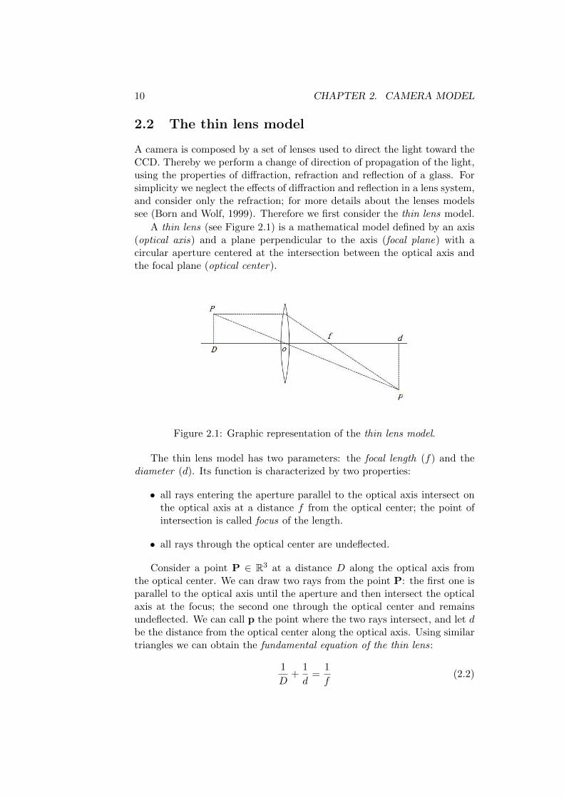
Figure 2.1: Graphic representation of the thin lens model.
The thin lens model has two parameters: the focal length (f) and thediameter (d). Its function is characterized by two properties:
• all rays entering the aperture parallel to the optical axis intersect onthe optical axis at a distance f from the optical center; the point ofintersection is called focus of the length.
• all rays through the optical center are undeflected.
Consider a point P ∈ R3 at a distance D along the optical axis fromthe optical center. We can draw two rays from the point P: the first one isparallel to the optical axis until the aperture and then intersect the opticalaxis at the focus; the second one through the optical center and remainsundeflected. We can call p the point where the two rays intersect, and let dbe the distance from the optical center along the optical axis. Using similartriangles we can obtain the fundamental equation of the thin lens:
1
D+
1
d=
1
f(2.2)
2.3. THE PINHOLE MODEL 11
Therefore the irradiance I(x) at the point x on the image plane is ob-tained by integrating all the energy emitted from the region of space thatproject on the point x, compatibly with the geometry of the lens.
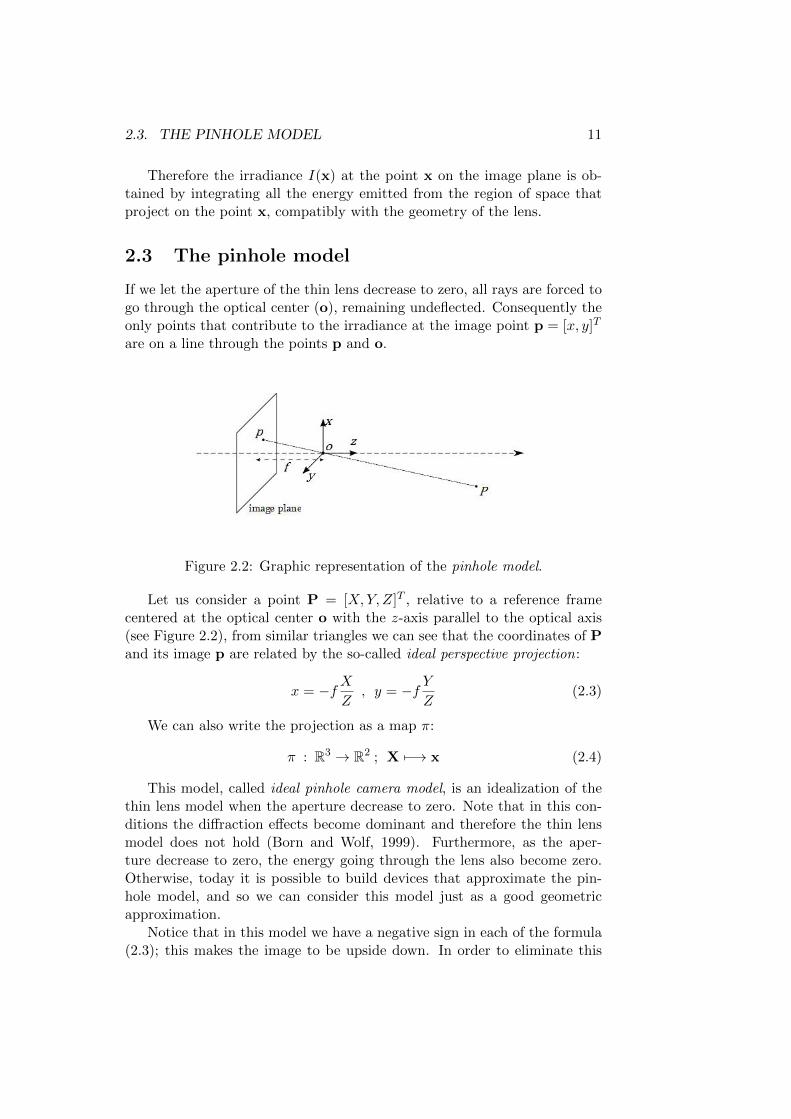
2.3 The pinhole model
If we let the aperture of the thin lens decrease to zero, all rays are forced togo through the optical center (o), remaining undeflected. Consequently theonly points that contribute to the irradiance at the image point p = [x, y]T
are on a line through the points p and o.
Figure 2.2: Graphic representation of the pinhole model.
Let us consider a point P = [X,Y, Z]T , relative to a reference framecentered at the optical center o with the z-axis parallel to the optical axis(see Figure 2.2), from similar triangles we can see that the coordinates of Pand its image p are related by the so-called ideal perspective projection:
x = −f XZ
, y = −f YZ
(2.3)
We can also write the projection as a map π:
π : R3 → R2 ; X 7−→ x (2.4)
This model, called ideal pinhole camera model, is an idealization of thethin lens model when the aperture decrease to zero. Note that in this con-ditions the diffraction effects become dominant and therefore the thin lensmodel does not hold (Born and Wolf, 1999). Furthermore, as the aper-ture decrease to zero, the energy going through the lens also become zero.Otherwise, today it is possible to build devices that approximate the pin-hole model, and so we can consider this model just as a good geometricapproximation.
Notice that in this model we have a negative sign in each of the formula(2.3); this makes the image to be upside down. In order to eliminate this
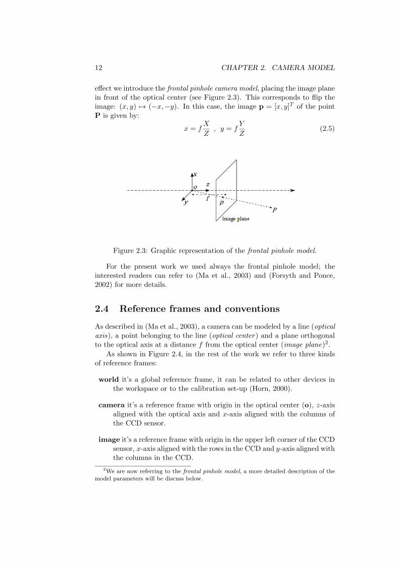
12 CHAPTER 2. CAMERA MODEL
effect we introduce the frontal pinhole camera model, placing the image planein front of the optical center (see Figure 2.3). This corresponds to flip theimage: (x, y) 7→ (−x,−y). In this case, the image p = [x, y]T of the pointP is given by:
x = fX
Z, y = f
Y
Z(2.5)
Figure 2.3: Graphic representation of the frontal pinhole model.
For the present work we used always the frontal pinhole model; theinterested readers can refer to (Ma et al., 2003) and (Forsyth and Ponce,2002) for more details.
2.4 Reference frames and conventions
As described in (Ma et al., 2003), a camera can be modeled by a line (opticalaxis), a point belonging to the line (optical center) and a plane orthogonalto the optical axis at a distance f from the optical center (image plane)2.
As shown in Figure 2.4, in the rest of the work we refer to three kindsof reference frames:
world it’s a global reference frame, it can be related to other devices inthe workspace or to the calibration set-up (Horn, 2000).
camera it’s a reference frame with origin in the optical center (o), z-axisaligned with the optical axis and x-axis aligned with the columns ofthe CCD sensor.
image it’s a reference frame with origin in the upper left corner of the CCDsensor, x-axis aligned with the rows in the CCD and y-axis aligned withthe columns in the CCD.
2We are now referring to the frontal pinhole model, a more detailed description of themodel parameters will be discuss below.
2.5. GEOMETRIC MODEL OF PROJECTION 13
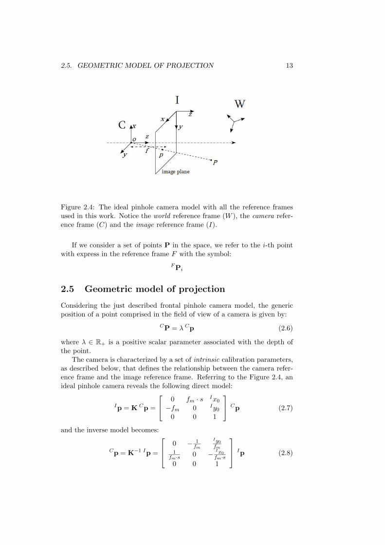
Figure 2.4: The ideal pinhole camera model with all the reference framesused in this work. Notice the world reference frame (W ), the camera refer-ence frame (C) and the image reference frame (I).
If we consider a set of points P in the space, we refer to the i-th pointwith express in the reference frame F with the symbol:
FPi
2.5 Geometric model of projection
Considering the just described frontal pinhole camera model, the genericposition of a point comprised in the field of view of a camera is given by:
CP = λ Cp (2.6)
where λ ∈ R+ is a positive scalar parameter associated with the depth ofthe point.
The camera is characterized by a set of intrinsic calibration parameters,as described below, that defines the relationship between the camera refer-ence frame and the image reference frame. Referring to the Figure 2.4, anideal pinhole camera reveals the following direct model:
Ip = K Cp =
0 fm · s Ix0
−fm 0 Iy0
0 0 1
Cp (2.7)
and the inverse model becomes:
Cp = K−1 Ip =
0 − 1fm
Iy0fm
1fm·s 0 − Ix0
fm·s0 0 1
Ip (2.8)
14 CHAPTER 2. CAMERA MODEL
where fm = f · Sx; s =Sy
Sx; Sx = pixels
length unit along x axis; Sy = pixelslength unit
along y axis3; (x0, y0) are the coordinates of the principal point of the CCD,defined as the intersection between the principal axis and the image plane.
2.6 Camera parameters
Usually when we refer to camera calibration we mean the recovery of theprincipal distance (or focal length) f and the principal point (x0, y0)T inthe image plane; or, equivalently, recovery of the position of the center ofprojection (x0, y0, f)T in the camera reference frame. This is referred to asinterior orientation in photogrammetry; for us these will be the intrinsicparameters.
A calibration target can be used to recover, from the correspondencesbetween points in the space and points in the image, a relationship betweenthe camera (or image) reference frame and the world reference frame. Thisis referred to as exterior orientation in photogrammetry, for us these will bethe extrinsic parameters.
Since cameras often have appreciable geometric distortions, camera cal-ibration is often taken to include the recovery of power series coefficients ofthese distortions. Furthermore, an unknown scale factor in image samplingmay also need to be recovered, because scan lines are typically resampled inthe frame grabber, and so picture cells do not correspond discrete sensingelements.
In this work we have developed a calibration procedure based on Tsai’smethod (Horn, 2000). This method for camera calibration recovers the in-trinsic parameters, the extrinsic parameters, the power series coefficients fordistortion, and an image scale factor that best fit the measured image coor-dinates, corresponding to known target point coordinates. This is done instages, starting off with closed form least-squares estimates of some param-eters and ending with an iterative non-linear optimization of all parameterssimultaneously, using these estimates as starting values.
2.6.1 Intrinsic parameters
Interior Orientation is the relationship between camera reference frame andimage reference frame. Camera coordinates and image coordinates are re-lated by the matrix K in equation 2.7. As we can see, matrix K has fourdegrees of freedom. The problem of intrinsic parameters calibration is therecovery of x0, y0, fm and s.
This is the basic task of camera calibration. However in practice we alsoneed to recover the position and attitude of the calibration target in the
3Sx and Sy are defined with reference to the directions x and y in the camera referenceframe and not in the image one.

2.6. CAMERA PARAMETERS 15
camera coordinate system (extrinsic parameters).
2.6.2 Extrinsic parameters
Exterior Orientation is the relationship between world reference frame andcamera reference frame. The transformation from world to camera consistsof a rotation and a translation. This transformation has six degrees offreedom (three for rotation and three for translation). The world coordinatesystem can be any system convenient for the particular design of the target.
The relationship between these two reference frames is given by:
WP =W RCCP +W TC (2.9)
where WRC is the rotation matrix from camera reference frame to worldreference frame, and WTC is the position of the origin of camera referenceframe expressed in world frame.
The problem of extrinsic parameters calibration is the recovery of threerotation angles, used to generate the rotation matrix, and three coordinatesof translation.
2.6.3 Distortion
Projection in an ideal imaging system is governed by the frontal pinholemodel. Real optical systems suffer from a number of inevitable geometricdistortions. In optical systems made of spherical surfaces, with centers alongthe optical axis, a geometric distortion occurs in the radial direction. Apoint is imaged at a distance from the principal point that is larger (pin-cushion distortion) or smaller (barrel distortion) than the predicted oneby the perspective projection equations; the displacement increasing withdistance from the center. It is small for directions that are near parallel tothe optical axis, growing as some power series of the angle. The distortiontends to be more noticeable with wide-angle lenses than with telephotolenses.
The displacement due to radial distortion can be modelled using theequations:
δx = x(κ1r2 + κ2r
4 + . . .)δy = y(κ1r
2 + κ2r4 + . . .)
(2.10)
where x and y are measured from the center of distortion, which is typicallyassumed to be at the principal point. Only even powers of the distance rfrom the principal point occur, and typically only the first, or perhaps thefirst and the second term in the power series are retained.
Equivalently we can express this distortion as function of r as:
δr = κ1r3 + κ2r
5 + . . . (2.11)
16 CHAPTER 2. CAMERA MODEL
Electro-optical systems typically have larger distortions than optical sys-tems made of glass. They also suffer from tangential distortion, which is atright angle to the vector from the center of the image. Like radial distortion,tangential distortion grows with distance from the center of distortion.
δx = −y(ε1r2 + ε2r
4 + . . .)δy = +x(ε1r
2 + ε2r4 + . . .)
(2.12)
In calibration, we attempt to recover the coefficients (κ1, κ2 , . . ., ε1, ε2,. . .) of these power series.
In this work we consider only the radial distortions because of the tan-gential distortions are negligible.
Chapter 3
Geometry of two cameras
A stereo system comprises two cameras, that we can call cam-1 and cam-2,that frame the same field of view. The geometry of stereo systems is basedon the epipolar geometry. In this chapter we describe the epipolar geometryand the triangulation process.
3.1 Epipolar geometry
Consider two images of the same scene taken from two distinct vantagepoints. If we assume that the cameras are calibrated, we know the posi-tion and orientation of the two camera frames with reference to the worldframe (see Section 2.6), and therefore the relative orientation and translationbetween the two camera frames.
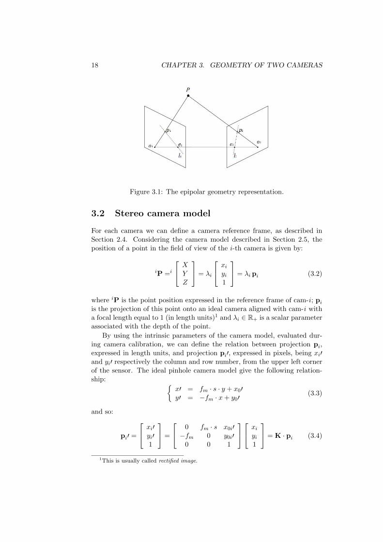
The intersections of the line (o1,o2) with each image plane are calledepipoles and denoted by e1 and e2 (see Figure 3.1). Consider a point P inthe 3D space in the field of view of both cameras; we can define the epipolarplane as the plane through P, o1 and o2. Notice that the projections ofpoint P on the image planes belong to the rays (o1,P) and (o2,P), bothbelonging to the epipolar plane; therefore the projections belongs to theepipolar plane too.
The lines l1 and l2 are called epipolar lines, which are the intersectionsof the epipolar plane with the two image planes.
Mathematically this considerations are expressed by the epipolar con-straint :
〈p2,T×Rp1〉 = 0 (3.1)
where (R,T) is the relative pose between the two cameras.The power of this constraint is applied to the matching of feature points
between the two images. Once we have the projection p1 of the point P onthe image plane π1, we have a description of the epipolar plane (o1,o2,p1)and so we can compute the epipolar line on image plane π2. The projectionp2 of the point P on the image plane π2 must belong to this line.
17
18 CHAPTER 3. GEOMETRY OF TWO CAMERAS
Figure 3.1: The epipolar geometry representation.
3.2 Stereo camera model
For each camera we can define a camera reference frame, as described inSection 2.4. Considering the camera model described in Section 2.5, theposition of a point in the field of view of the i-th camera is given by:
iP =i
XYZ
= λi
xiyi1
= λi pi (3.2)
where iP is the point position expressed in the reference frame of cam-i ; piis the projection of this point onto an ideal camera aligned with cam-i witha focal length equal to 1 (in length units)1 and λi ∈ R+ is a scalar parameterassociated with the depth of the point.
By using the intrinsic parameters of the camera model, evaluated dur-ing camera calibration, we can define the relation between projection pi,expressed in length units, and projection pi′, expressed in pixels, being xi′and yi′ respectively the column and row number, from the upper left cornerof the sensor. The ideal pinhole camera model give the following relation-ship:
x′ = fm · s · y + x0′y′ = −fm · x+ y0′
(3.3)
and so:
pi′ =
xi′yi′1
=
0 fm · s x0i′−fm 0 y0i′
0 0 1
xiyi1
= K · pi (3.4)
1This is usually called rectified image.

3.3. TRIANGULATION 19
where fm = f · Sx; s =Sy
Sx; Sx = pixels
length unit along x axis; Sy = pixelslength unit
along y axis2.
3.3 Triangulation
The algorithm used for computing the depth of a point in the field of viewof both cameras in a stereo-pair is called triangulation. In the followingparagraphs we present the ideal case of triangulation and, later, the real casewith the middle point approach. More complex approaches, like epipolaroptimization algorithm, are described in (Ma et al., 2003).
3.3.1 Ideal case
When a point in space is in the field of view of both cameras in a stereo-pair,the rays through the optical center and the projection of the point on theimage plane of each cameras intersect in the point itself.
Figure 3.2: The triangulation geometry in an ideal case.
With reference to Figure 3.2, the rays through (o1, p1) and (o2, p2) in-tersect exactly in the point P . In mathematical language it can be expressas:
WP = λ1(Wp1 − Wo1) = λ2(Wp2 − Wo2) (3.5)
This is a system of three equations in two variables (λ1 and λ2) but, in thisideal case, there are only two linearly independent equations. The positionof the point P will be computed from one of the rays in Equation 3.5.
2Notice that the parameters Sx and Sy are referred to x and y-axis and not to x′ andy′-axis.
20 CHAPTER 3. GEOMETRY OF TWO CAMERAS
3.3.2 Real case
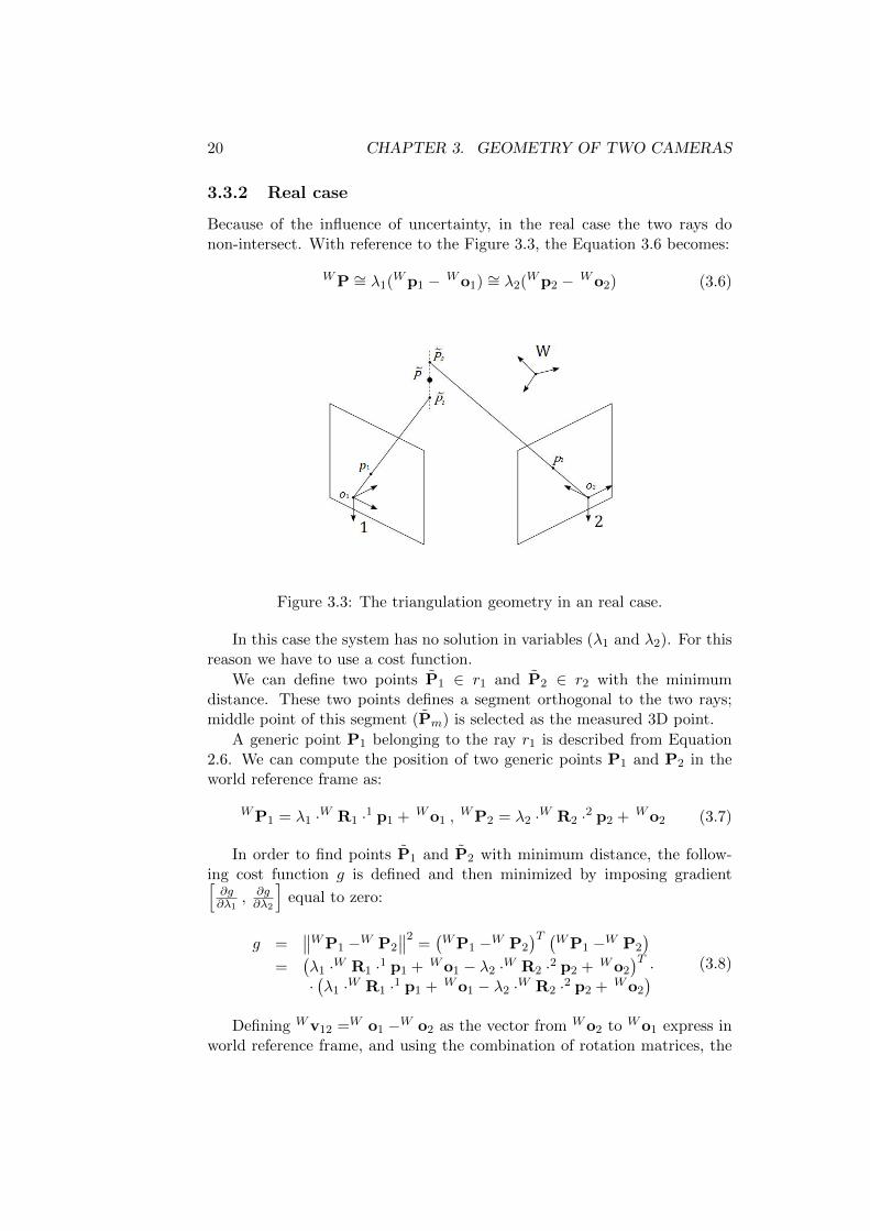
Because of the influence of uncertainty, in the real case the two rays donon-intersect. With reference to the Figure 3.3, the Equation 3.6 becomes:
WP ∼= λ1(Wp1 − Wo1) ∼= λ2(Wp2 − Wo2) (3.6)
Figure 3.3: The triangulation geometry in an real case.
In this case the system has no solution in variables (λ1 and λ2). For thisreason we have to use a cost function.
We can define two points P1 ∈ r1 and P2 ∈ r2 with the minimumdistance. These two points defines a segment orthogonal to the two rays;middle point of this segment (Pm) is selected as the measured 3D point.
A generic point P1 belonging to the ray r1 is described from Equation2.6. We can compute the position of two generic points P1 and P2 in theworld reference frame as:
WP1 = λ1 ·W R1 ·1 p1 + Wo1 ,WP2 = λ2 ·W R2 ·2 p2 + Wo2 (3.7)
In order to find points P1 and P2 with minimum distance, the follow-ing cost function g is defined and then minimized by imposing gradient[∂g∂λ1
, ∂g∂λ2
]equal to zero:
g =∥∥WP1 −W P2
∥∥2=(WP1 −W P2
)T (WP1 −W P2
)=
(λ1 ·W R1 ·1 p1 + Wo1 − λ2 ·W R2 ·2 p2 + Wo2
)T ··(λ1 ·W R1 ·1 p1 + Wo1 − λ2 ·W R2 ·2 p2 + Wo2
) (3.8)
Defining Wv12 =W o1 −W o2 as the vector from Wo2 to Wo1 express inworld reference frame, and using the combination of rotation matrices, the

3.3. TRIANGULATION 21
Equation 3.8 becomes:
g = λ21 ·1 pT1 ·1 p1 − 2 · λ1 · λ2 ·1 pT1 ·1 R2
2p2 − 2 · λ1 ·1 pT1 ·1 v21+−2 · λ2 ·2 pT2 ·2 v12 + λ2
2 ·2 pT2 ·2 p2 +W vT12 ·W v12
(3.9)Taking partial derivatives and assigning a value of zero to the gradient
yields the following equation system:∂g∂λ1
= λ1
(2 1p1
T 1p1
)+ λ2
(−2 1p1
T 1R22p2
)+(−2 1p1
T 1v21
)= 0
∂g∂λ2
= λ1
(−2 1p1
T 1R22p2
)+ λ2
(2 2p2
T 2p2
)+(−2 2p2
T 2v12
)= 0
(3.10)The solution of this system are the λ1 and λ2 values that define the
minimum distance segment between the two rays. The symbolic solution ofthe system is:
λ1 =
(1p1
T ·1R2·2p2
)·(2p2
T ·2v12
)+(2p2
T ·2p2
)·(1p1
T ·1v21
)(1p1
T ·1p1)·(2p2T ·2p2)−(1p1
T ·1R2·2p2)2
λ2 =
(1p1
T ·1p1
)·(2p2
T ·2v12
)+(1p1
T ·1R2·2p2
)·(1p1
T ·1v21
)(1p1
T ·1p1)·(2p2T ·2p2)−(1p1
T ·1R2·2p2)2
(3.11)
Thus, the extreme points P1 and P2 of the minimum distance segmentare:
W P1 = λ1 · WR1 · 1p1 + Wo1 ,W P2 = λ2 · WR2 · 2p2 + Wo2 (3.12)
and the middle point associated with the points is:
W Pm =W P1 + W P2
2(3.13)

22 CHAPTER 3. GEOMETRY OF TWO CAMERAS

Part II
Proposed algorithms
23

Chapter 4
Algorithm for staticreconstruction
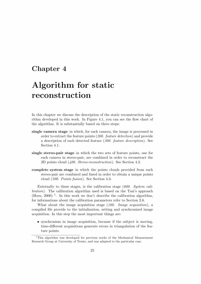
In this chapter we discuss the description of the static reconstruction algo-rithm developed in this work. In Figure 4.1, you can see the flow chart ofthe algorithm. It is substantially based on three steps:
single camera stage in which, for each camera, the image is processed inorder to extract the feature points (200. feature detection) and providea description of each detected feature (300. feature description). SeeSection 4.1.
single stereo-pair stage in which the two sets of feature points, one foreach camera in stereo-pair, are combined in order to reconstruct the3D points cloud (400. Stereo-reconstruction). See Section 4.2.
complete system stage in which the points clouds provided from eachstereo-pair are combined and fused in order to obtain a unique pointscloud (500. Points fusion). See Section 4.3.
Externally to these stages, is the calibration stage (600. System cali-bration). The calibration algorithm used is based on the Tsai’s approach(Horn, 2000) 1. In this work we don’t describe the calibration algorithm,for informations about the calibration parameters refer to Section 2.6.
What about the image acquisition stage (100. Image acquisition), acompiled file provide to the initialization, setting and synchronized imageacquisition. In this step the most important things are:
• synchronism in image acquisition, because if the subject is moving,time-different acquisitions generate errors in triangulation of the fea-ture points.
1This algorithm was developed for previous works of the Mechanical MeasurementResearch Group at University of Trento, and was adapted to the particular case.
25
26 CHAPTER 4. ALGORITHM FOR STATIC RECONSTRUCTION
Figure 4.1: Functional description of the algorithm for static 3D reconstruc-tion
• settings of camera parameters, because different settings of two cam-eras in a single stereo-pair can provide different feature descriptionsand so errors in feature matching.
4.1 Feature extraction
The colored circular markers in the image shall be recognized in order to cre-ate a list of descriptor array. The image segmentation algorithm is based onedge detection using Canny operator (Canny, 1986). The feature extractionalgorithm proposed in this work is composed of two steps: feature detection,which refers to the edge detection and filtering in order to select only thecolored markers, and feature description, which refers to the generation ofan array of descriptors used in the feature matching stage.
4.1.1 Feature detection
We start from an RGB image and we transform it into a gray-scale image inorder to compute the edges using the Canny algorithm. In literature thereare a lot of edge detectors (sobel, roberts, . . . ), but we chose the canny onebecause of it is the best way to obtain closed contours. Thus we have abinary image that represents the contours of the markers but also contoursof other objects in the field of view of the camera, and so we have to filter
4.1. FEATURE EXTRACTION 27
the image.In the binary image we can consider each set of connected pixel as a
distinct object. In this way we have a set of objects in the image and wehave to determine if they are markers or not markers. For each object wecan compute a set of geometric parameters:
Euler Number It is a scalar value that represents the total number ofobjects in the image minus the total number of holes in those objects.Since we consider one object singularly, the Euler number can be 1, ifthe contour is open; 0, if the object has only one hole; or less then 0,if the object has more then one hole.
Area It is the number of pixels in the object. In this case the object is thecontour of a real object in the scene and so this value could be theperimeter of the marker.
Filled Area It is the area of the object plus the area of all the holes in theobject. In this case this value could represents the area of the marker.
Major Axis Length It is a scalar value specifying the length (in pixels)of the major axis of the ellipse that has the same normalized secondcentral moments as the region.
Minor Axis Length It is a scalar value specifying the length (in pixels)of the minor axis of the ellipse that has the same normalized secondcentral moments as the region.
Using these parameters we can select two conditions in order to establish ifthe object is the contour of a marker or something else.
The first condition is that the recognized object shall be closed contourwith a single hole inside. This condition is mathematically described by;
EulerNumber = 0
The second condition is based on the consideration that the projection ofa circle, although deformed, is approximately an ellipse; so the ratio betweenperimeter and area must be, within a certain tolerance:
Area
FilledArea=
√2 · (a2 + b2)
ab± tolerance
where a = MajorAxisLength and b = MinorAxisLength. The tolerance isrelated to two reasons: first, image digitalization and edge detection makethe ellipse perimeter a polynomial approximation. Second, the exact for-mula of ellipse circumference is C = 4aE(ε), where the function E(·) is thecomplete elliptic integral of the second kind and ε is the eccentricity; theformula used in this work is an approximation with about 5% of tolerance(Barnard et al., 2001).
28 CHAPTER 4. ALGORITHM FOR STATIC RECONSTRUCTION
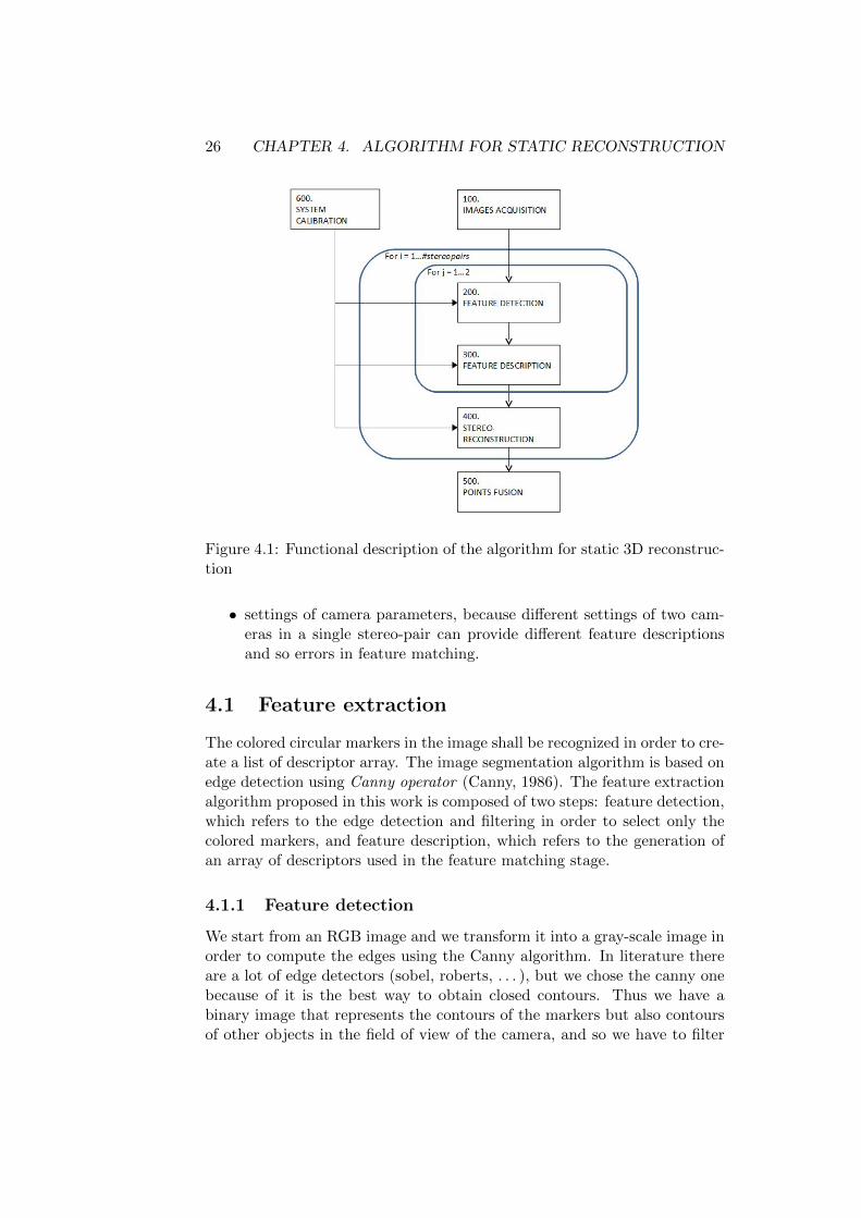
If both these conditions are verified, the object is considered as a marker,otherwise it will be deleted. An example of the image segmentation processis shown in Figure 4.2.
(a) original image (b) gray-scale image
(c) Canny edges (d) marker detected
Figure 4.2: The image segmentation process. The original image in RGBcomponents is converted in gray scale and the edges are determined by usingCanny algorithm. The object are filtered in order to delete the one withoutholes and the one that is not an ellipse.
4.1.2 Feature description
In order to determine the correspondence between feature points in twocamera of the same stereo-pair, we have to generate a complete description ofthe feature point in term of position, geometry and chromatic characteristics.Each marker is described from:
centroid the position of the marker’s centroid expressed in image referenceframe.
shape an array of four parameters that describes the geometric character-istics of the marker; these parameters are: the area of the coloredmarker, its eccentricity, its orientation and the major axis length.
color a scalar value that indicates the color of the marker.
stripe a scalar value that indicates the stripe which the marker belongs.
4.2. STEREO-RECONSTRUCTION 29
The colors of the markers are assumed to be known a priori. We cancompute the mean RGB components of pixels belonging to the marker. Weassociate the marker to a color class by using, in sequence, the k-meansalgorithm and nearest neighbor algorithm. In order to minimize the miss-classification, we used only four colors, equispaced in the (a*,b*) plane ofthe CIE-L*a*b* color space (ISO 12640-3:2007, 2007).In our case we choosethe colors: red, green, blue and yellow.
The stripes clustering is performed on the same color markers and thealgorithm is based on principal component analysis.
4.2 Stereo-reconstruction
Once we have detected all the features in two images of the same stereo-pair, we can proceed to 3D reconstruction. This stage can be divided intwo subproblems: feature matching and triangulation. What about thetriangulation algorithm, we refer to the middle point approach, as describedin Section 3.3.
The general approach to the feature matching for marker systems is theminimum epipolar distance approach. Let us consider the feature point PLin the left image of the stereo-pair, from the calibration parameters we cancompute the equation of the epipolar line on the right image. The standardalgorithm associates with the point PL the point PR in the right image withthe same color of PL and the minimum distance to the epipolar line. Whenapplied to our system, this approach shows two different problems:
• if the angle between the epipolar line and the stripes direction is small,the association is highly sensible to the noise in the centroid determi-nation.
• if the epipolar line intersect a lot of stripes, the probability to have awrong association will be very high (about 50%).
For a more robust association we can use, instead of the distance to theepipolar line, a cost function (g(·)) of the descriptors of the feature point.With reference to the Section 4.1.2, we define the cost function as:
g(PL, PR) = KE ·DE(PL, PR) +KS · ‖shape(PL)− shape(PR)‖ (4.1)
where DE(PL, PR) is the distance of point PR to the epipolar line generatedfrom PL, shape(P ) is the four elemets array of shape descriptors, and KE
and KS are two scalar coefficients that shall be tuned for the system.Also using the cost function, the association is still affected by miss-
match. In order to have an association as robust as possible, an innovativealgorithm is proposed in this work. This algorithm is based on two differentsteps: the determination of a correct starting point and the expansion fromthis point with a threshold on the disparity gradient.

30 CHAPTER 4. ALGORITHM FOR STATIC RECONSTRUCTION
4.2.1 Finding the starting stripe
Let us consider two set of feature points ΣL and ΣR, respectively relatedto left and right images. To each point PL ∈ ΣL we associate the pointPR ∈ ΣR that has:
• the same color of the point PL,
• the minimum value of the function g(·).
For each pair (PL, PR) we have a corresponding pair of stripes (sL, sR),where PL ∈ sL and PR ∈ sR. To each stripe sL we can associate the stripesR that has the maximum number of matched points, and a score thatrepresents the percentage of points of sR associated with the ones in sL.The starting stripe is the pair (sL, sR) with the maximum score.
4.2.2 Expansion from starting stripe
Once we have the starting stripes association, we have a set of matched pairs(PL, PR) and, to each pair is associated a disparity value, defined as the dif-ference of coordinates of PL and PR, both expressed in own image referenceframe. As explained in (Hartley and Zisserman, 2004), the disparity valueis directly related to the depth of the point from the cameras. If we considerthat the object is a continuous surface, we can impose the continuity of thedisparity map.
In practice we proceed in an iterative loop that provides:
• determination of the N feature points in the left image nearest to theones already matched.
• to each point, we associate the feature point in the right image having:
– the same color of the point PL,
– the minimum value of the function g(·),
– disparity in the range [d0 −∆d, d0 + ∆d].
where d0 is the disparity of the nearest point to the analyzed one, and ∆d
is a parameter of the algorithm that is related to the maximum variation ofdepth acceptable. If there are no points in the range, the feature point isconsidered without matching.
The iterative loop ends when all the points in the left image are matchedto one in the right image.
4.3. POINTS FUSION 31
4.3 Points fusion
One of the most critical point in the multiple stereo approach, is originatedfrom the fact that the points cloud is generated from several different stereo-pairs, and so we need a final stage in order to fuse the single points cloudsin a unique one.
All the existing approaches are based on the partial overlapping of thepoints clouds, and provide a registration of the different clouds. The mostcommon approaches are Iterative Closest Points (ICP) (Trucco et al., 1999;Eggert et al., 1997), and Bundle Adjustment (BA) (Triggs et al., 2000),often used in sequence.
In this work we propose a method for points fusion based on the uncer-tainty propagation by using the jacobian matrix, a compatibility analysisby using Mahalanobis distance and a Bayesian data fusion.
4.3.1 Uncertainty analysis
In the triangulation algorithm described above, the triangulated point Pm
is computed as a function of:
• the projection of 3D point on the image plane of each camera (Ipi, 2components each)
• the intrinsic calibration parameters of each camera (Ki, 4 componentseach)
• the extrinsic calibration parameters of each camera (WRi and Woi, 6components each)
And so the coordinates of point Pm are a function of 24 parameters
Pm = f(Ip1,
Ip2,K1,K2,WR1,
WR2,Wo1,
Wo2
)︸ ︷︷ ︸24 parameters
(4.2)
The rotation matrix is a 3 × 3 matrix and so it has 9 elements but,as we know from the rigid body transformation rules (Ma et al., 2003),the matrix has only three degrees of freedom. Each rotation matrix can beconveniently expressed by a set of three Euler angles (αi, βi and γi) definingrotation around three different axis (Goldstein et al., 2001).
In the sections below we discuss the evaluation of the uncertainty ineach of these parameters, considering the calibration process and the featuredetection process. After that we discuss the propagation of these uncertaintyin order to evaluate the covariance matrix of 3D point position.
32 CHAPTER 4. ALGORITHM FOR STATIC RECONSTRUCTION
Calibration uncertainty
The parameters characterizing the camera model are estimated in a cameracalibration stage, the procedure used is similar to that proposed by Tsai(Horn, 2000). The proposed procedure use a planar target which trans-lates orthogonal to itself, generating a three-dimensional grid of calibrationpoints. At a first step, the parameters are evaluated by a pseudo-inverse so-lution of a least-squares problem employing points on the calibration volumeand image points. A second step provides an iterative optimization in orderto minimize errors between acquired image points and the projections of the3D calibration points on the image plane with the estimated parameters.
Before the calibration algorithm can be applied, optical radial distortionare estimated and adjusted by rectifying distorted images. Radial distortioncoefficients are estimated by compensation of the curvature induced by radialdistortion on the calibration grid (Devernay and Faugeras, 2001).
Camera parameters uncertainties are evaluated propagating by the un-certainties of the 3D calibration points and those of image points (Chenet al., 2008; Horn, 2000). A Monte Carlo simulation is used.
The reasons of the deviation between measured image points and theprojection of 3D calibration points are various:
• simplification in camera model;
• digital camera resolution;
• dimensional accuracy of the calibration grid;
• geometrical and dimensional accuracy of grid translation.
In particular, if the motion of the grid to generate the calibration vol-ume is not perfectly orthogonal to the optical axis of the camera, a bias isinduced in the uncertainty distribution of the grid points, so that the uncer-tainty becomes non-symmetric in the image plane. Two more parameters aretherefore introduced to characterize the horizontal and vertical deviationsfrom orthogonality, αR and βC are the angles between translation directionand, respectively, grid rows and columns. In an ideal grid motion the twoparameters shall be 90.
Summarizing, the calibration routine consists of the following four steps:
1. Estimation and adjustment of the optical radial distortions.
2. First estimation of the parameters αR and βC , defining the imper-fection of the calibration target motion. These values are achievedby minimizing iteratively the deviation between the measured imagecoordinates of calibration points and those reconstructed projectingvolume points. The principal point is assumed to lie in the middle
4.3. POINTS FUSION 33
point of the image. With this assumption, once the systematic devia-tion from orthogonality have been compensated, extrinsic and intrinsicparameters can be derived from a pseudo inverse solution (Horn, 2000).
3. Final iterative optimization of all camera parameters (including prin-cipal point) is performed, iteratively minimizing the deviation betweenmeasured image points and those reconstructed projecting the 3D cal-ibration points. This step supplies the final estimation of intrinsic andextrinsic parameters. Standard deviation of the residuals after theprojection is combined with the resolution uncertainty, and is used toevaluate the uncertainty associated with the image points used in thenext step.
4. Lastly, through a Monte Carlo simulation, the uncertainties of theimage points (as evaluated in the previous step) and the 3D calibra-tion points are propagated, in order to evaluate the uncertainty of thecalibration parameters.
Steps 2 and 3 usually require usually less than 10 iterations, while theMote Carlo simulation step usually require about 105 iterations.
Feature uncertainty
The point P in 3D is defined as the centroid of a circular marker; for thisreason, determination of its projection pi in the image plane of the i-thcamera is always affected by uncertainty. First of all, digitalization and suc-cessive binarization of the image deforms the circular shape into a polygonalshape, and the centroid of these two shapes is not the same. Second, themarker, which was originally a circle, is deformed in order to adhere to thetarget surface; as first approximation, the deformed marker can be expressas an ellipse. Third, due to perspective effects, an ellipse which is not per-pendicular to the optical axis of the camera is projected on the CCD as anovoid.
A simplified model of the perspective geometry identifies each markerprojection as an ellipse; this ellipse can be fitted by the covariance matrix ofthe distribution of the pixels recognized as markers. The projected markercan then be compared with the corresponding covariance ellipse and the 2Ddistance of the two boundaries (∆b) can be computed as a function of angleα. This distribution ∆b(α) = breal(α) − ffit(α) is a map R −→ R2. Figure4.3 shows an example of a badly segmented elliptical marker and the fittedone, and the related distribution ∆b.
Two parameters ∆C and Cb, which express the “difference” betweenthe projected ovoid and the estimated ellipse can be computed; ∆C =[x∆C
, y∆C]T ∈ R2 is the displacement between the centroid of the segmented

34 CHAPTER 4. ALGORITHM FOR STATIC RECONSTRUCTION
Figure 4.3: Example of badly segmented elliptical marker. On the left, theedge of the marker and the fitted ellipse; on the right, the distribution ∆b.
marker and the fitted ellipse, and Cb ∈ R2×2 is the covariance matrix of dis-tribution ∆b.
The uncertainty of the centroid of the segmented marker is representedby a covariance matrix which is a function of these two parameters:
Umeas = f (∆C , Cb) = a ·[x∆C
00 y∆C
]+ b · Cb (4.3)
The larger the difference between the projected ovoid and the estimatedellipse, the larger the uncertainty associated with the computed centroid. Inthis function, parameters a and b are evaluated by a calibration procedure,which uses a grid of circular photolithographic markers. This grid is movedin a set of known positions and orientations, and the computed centroidof the segmented marker is compared with the projected reference on theCCD. In order to have a large set of views, two kinds of grids are used: thefirst is a planar surface and the second the lateral surface of a cylinder.
4.3.2 Uncertainty propagation
The uncertainty evaluation for triangulated point Pm of each stereo pairbecomes an uncertainty propagation problem, which employs the functionalmodel between input and output quantities, as express in Equation 4.2.
Several uncertainty propagation methods are known. Each of them isbased on a theory (i.e. probability, possibility or evidence theory), whichcan express uncertainty by a corresponding suitable means (i.e. probabilitydensity functions, fuzzy variables or random-fuzzy variables). According tothe GUM (BIPM et al., 1993), in this work, the uncertainty is analyzedaccording to the probability theory and is expressed by probability densityfunctions (PDFs).
In order to calculate the propagated uncertainty of triangulated posi-tion Pm, taking into account the contributions of all uncertainty sources,the method based on the formula expressed in the GUM is used. Thismethod is selected instead, for example, of the Monte Carlo propagationapproach, in order to increase computing speed and to allow real-time com-
4.3. POINTS FUSION 35
puting implementation. The propagation formula uses the sensitivity coeffi-cients obtained from linearization of the mathematical model; this methodis based on thee hypothesis that a probability distribution, assumed or ex-perimentally determined, can be associated with every uncertainty sourceconsidered, and that a corresponding standar uncertainty can be obtainedfrom the probability distribution.
The GUM proposes a formula for the calculation of the uncertainty tobe associated with output quantities Pm, obtainable as an indirect measure-ment of all input quantities:
Uout = c ·Uin · cT (4.4)
where Uin ∈ R24×24 is the covariance matrix associated with the input quan-tities, which are 24 in this application; Uout ∈ R3×3 is the covariance matrixassociated with the output quantities, which are the three components ofPm in this application; and c ∈ R3×24 is the matrix of the sensitivity co-efficients achievable from partial derivatives of f(·) with respect to inputvariables:
ci,j =∂fi
∂inputj(4.5)
In this application, the following assumptions are made:
1. The two components of the projected point Ipi of each camera areassumed to be cross-correlated among themselves and not correlatedwith any other input quantity.
2. The intrinsic calibration parameters of each camera are assumed to becross-correlated among themselves and not correlated with the corre-sponding parameters of the other cameras or any other input quantity.
3. The extrinsic calibration parameters of each camera are assumed to becross-correlated among themselves and not correlated with the corre-sponding parameters of the other cameras or any other input quantity.
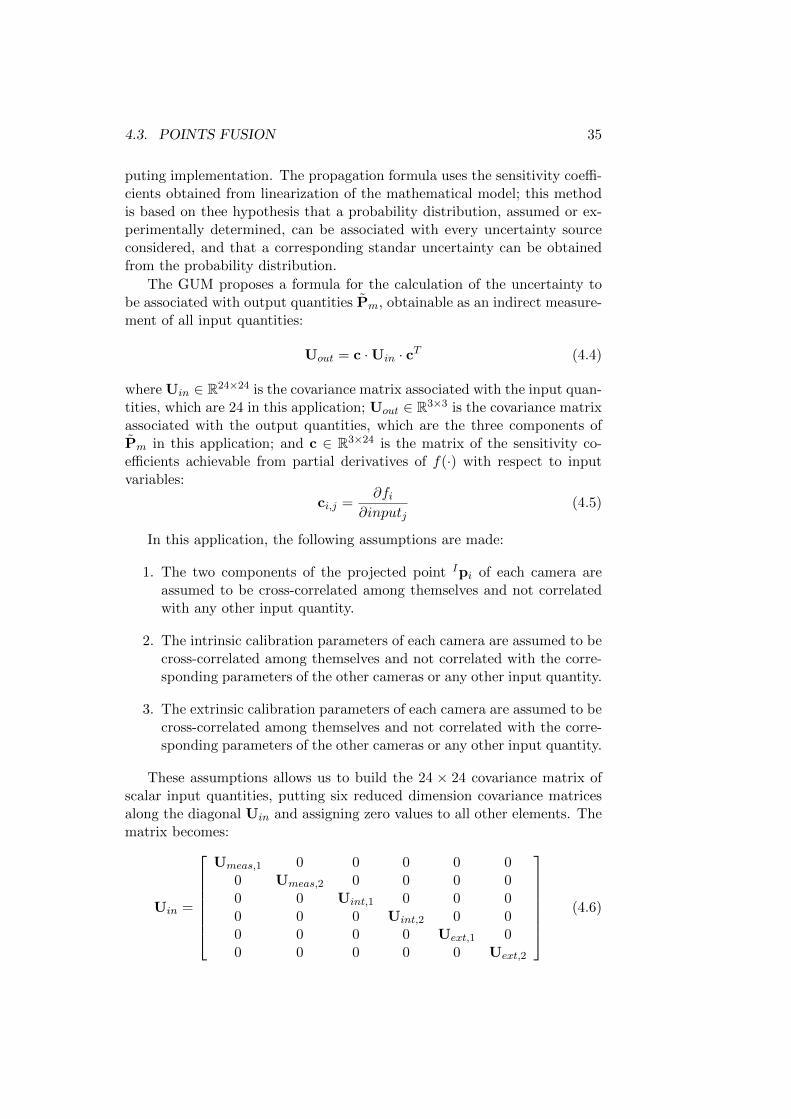
These assumptions allows us to build the 24 × 24 covariance matrix ofscalar input quantities, putting six reduced dimension covariance matricesalong the diagonal Uin and assigning zero values to all other elements. Thematrix becomes:
Uin =
Umeas,1 0 0 0 0 00 Umeas,2 0 0 0 00 0 Uint,1 0 0 00 0 0 Uint,2 0 00 0 0 0 Uext,1 00 0 0 0 0 Uext,2
(4.6)
36 CHAPTER 4. ALGORITHM FOR STATIC RECONSTRUCTION
where Umeas,i ∈ R2×2 is the covariance matrix associated with measurementof the projected point Ipi in the i-th camera; Uint,i ∈ R4×4 is the covariancematrix associated with the intrinsic calibration parameters of the i-th cam-era; and Uext,i ∈ R6×6 is the covariance matrix associated with the extrinsiccalibration parameters of the i-th camera.
The propagation model between input and output quantities describedin this work is not very simple, but have the advantage of being explicit.Thus, it is possible to compute explicitly the sensitive coefficients as symbolicexpressions, and it is not necessary to evaluate them numerically, as oftenhappens with complex applications.
4.4 Compatibility analysis
As we have seen in Section 4.3.1, in non-ideal conditions, the stereo systemsat different positions provide different measurements of the same featurepoint; in this work the feature points are centroids of colored spots. Eachmeasurement comes with its uncertainty, and a fusion process can combinethem in a single best-estimated one with the associated fused uncertainty.Before points measured from different stereo systems can be fused, it isnecessary to state whether they are associated with the same feature or,statistically speaking, whether they belong to the same distribution. Acompatibility analysis of the measured points is therefore performed.
A compatibility test on two points P1 and P2, with covariances C1 andC2, is based on the consideration that the difference P1 −P2 is distributedwith zero mean and covariance C = C1 + C2.
We can define the Mahalanobis Distance (MD) (Duda et al., 2000) as astatistical distance described by the equation:
MD2 = (P1 −P2)T (C1 + C2)−1(P1 −P2) (4.7)
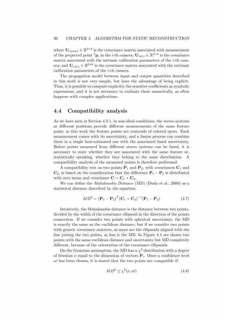
Intuitively, the Mahalanobis distance is the distance between two points,divided by the width of the covariance ellipsoid in the direction of the pointsconnection. If we consider two points with spherical uncertainty, the MDis exactly the same as the euclidean distance; but if we consider two pointswith generic covariance matrices, as more are the ellipsoids aligned with theline joining the two points, as less is the MD. In Figure 4.4 are shown twopoints with the same euclidean distance and uncertainty but MD completelydifferent, because of the orientation of the covariance ellipsoids.
On the Gaussian assumption, the MD has a χ2 distribution with a degreeof freedom ν equal to the dimension of vectors Pi. Once a confidence levelα′ has been chosen, it is stated that the two points are compatible if:
MD2 ≤ χ2(ν, α′) (4.8)
4.4. COMPATIBILITY ANALYSIS 37
Figure 4.4: An example of different Mahalanobis Distance between the samecouple of points, with covariance ellipsoids of equal axis length but differentorientations. In the first case (a) the MD is equal to 4.5, in the second one(b) is 0.36.
Let Pi,j be the i-th 3D point measured by the j-th stereo-pair withcovariance Ci,j . The point fusion algorithm is made up of the following steps:from measured points sets Σm and Σn of stereo-pairs m and n respectively,each point Pi,m ∈ Σm is associated with the point Pj,n ∈ Σn having theminimum MD; if the compatibility test is passed, the association is acceptedand the associated couple of points is fused, yelding the best estimate:
P∗k,mn = Cj,n(Ci,m + Cj,n)−1Pi,m + Ci,m(Ci,m + Cj,n)−1Pj,n (4.9)
and its covariance matrix:
C∗k,mn = Cj,n(Ci,m + Cj,n)−1Ci,m (4.10)
otherwise Pi,m and its covariance matrix Ci,m are kept as best estimate ofthe feature; the process between all these best estimates is iterated (includingpoints not associated between the two sets), and a new set Σp is obtained.
Ambiguous cases may occur, when a point of set Σn is compatible withtwo or more points of set Σm. In this case, the point of Σn is eliminated.For this reason, threshold α′ must be tuned in order both to keep cases ofambiguity low and not to lose useful information.
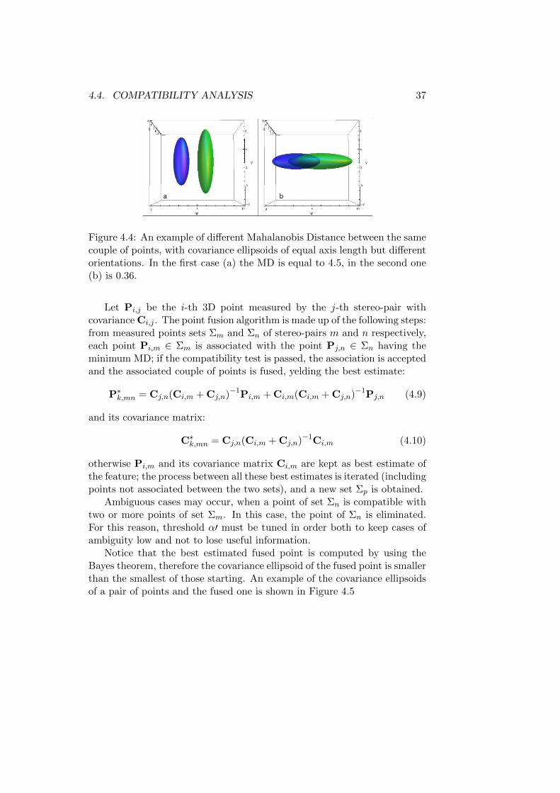
Notice that the best estimated fused point is computed by using theBayes theorem, therefore the covariance ellipsoid of the fused point is smallerthan the smallest of those starting. An example of the covariance ellipsoidsof a pair of points and the fused one is shown in Figure 4.5

38 CHAPTER 4. ALGORITHM FOR STATIC RECONSTRUCTION
Figure 4.5: An example of covariance ellipsoids of two corresponding pointsacquired by two stereo-pairs, and the ellipsoid of the fused point.
Chapter 5
Algorithm for MotionCapture
With the algorithm described in Chapter 4 we have a system able to capturea certain number of images from different cameras and, from this images,to reconstruct the 3D position of a certain number of feature points in thefield of view. In this case we acquire a single image for each camera.
If we acquire not only a single image, but a sequence of images, we canuse this time-variant information in order to characterize better the viewedobjects. In particular we are interested in the segmentation of the differentobjects in the field of view and in modeling the joints between these objects.
The final aim of the here presented system is to obtain a complete de-scription of the articulated body in 3D and its motion properties automati-cally from a set of images given a known pattern. In particular, our interestis on the analysis of human motion (i.e. arms or legs).
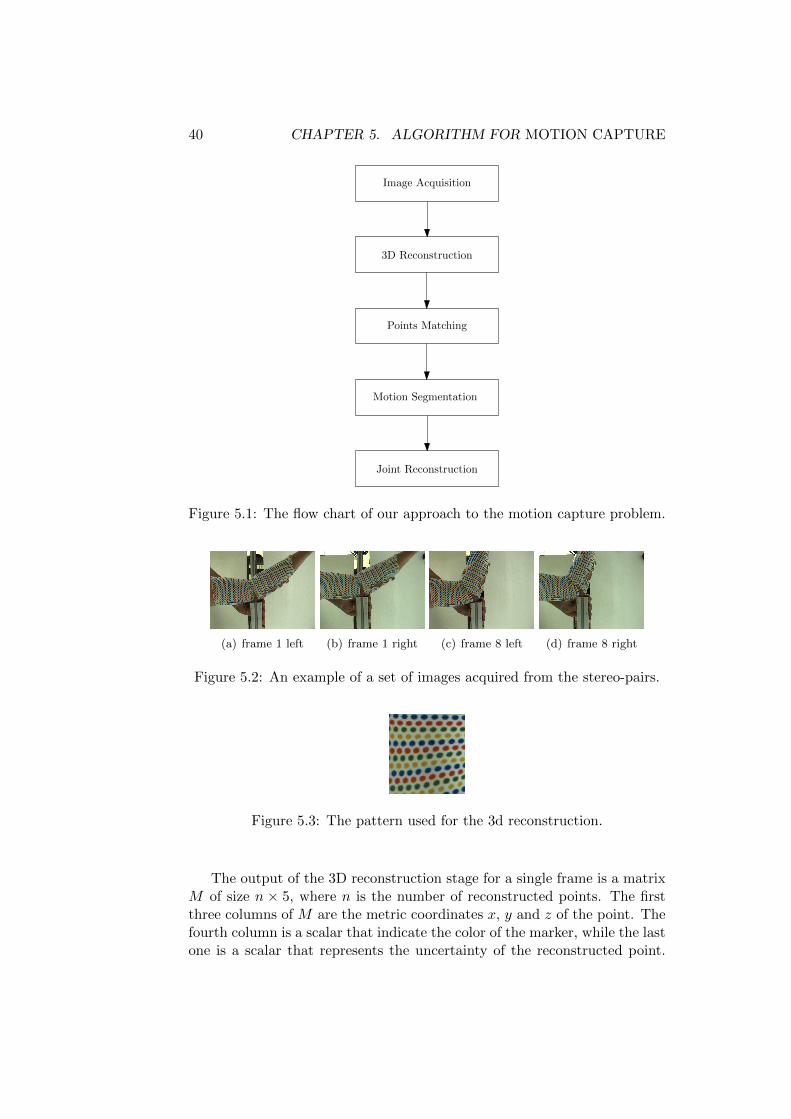
As graphically explained in Figure 5.1, the proposed algorithm is a se-quence of four steps. What about image acquisition and 3D reconstructionsteps we refer to Chapter 4, here we present only a brief reminder in Sec-tion 5.1. The next Section 5.2 shows how the pairwise 3D matching is doneexploiting the particular structure of the pattern. Section 5.3 presents thesegmentation algorithm based on the motion of the object shape, we de-scribe here three different algorithms: GPCA, RANSAC ans LSA. FinallySection 5.4 describes the articulated joint position computation.
5.1 Image acquisition and 3D reconstruction
The image acquisition system, by using the 3D static reconstruction algo-rithm described in Chapter 4, is able to reconstruct the position of a set ofpoints belonging to a generic surface located in a given working space.
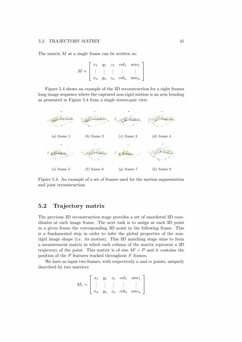
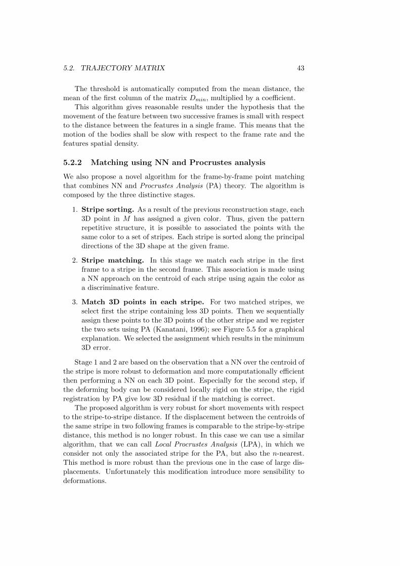
An example of a subset of acquired images is shown in Figure 5.2, to-gether with the pattern used for the acquisitions (Figure 5.3).
39
40 CHAPTER 5. ALGORITHM FOR MOTION CAPTURE
Image Acquisition
3D Reconstruction
Points Matching
Motion Segmentation
Joint Reconstruction
Figure 5.1: The flow chart of our approach to the motion capture problem.
(a) frame 1 left (b) frame 1 right (c) frame 8 left (d) frame 8 right
Figure 5.2: An example of a set of images acquired from the stereo-pairs.
Figure 5.3: The pattern used for the 3d reconstruction.
The output of the 3D reconstruction stage for a single frame is a matrixM of size n × 5, where n is the number of reconstructed points. The firstthree columns of M are the metric coordinates x, y and z of the point. Thefourth column is a scalar that indicate the color of the marker, while the lastone is a scalar that represents the uncertainty of the reconstructed point.
5.2. TRAJECTORY MATRIX 41
The matrix M at a single frame can be written as:
M =
x1 y1 z1 col1 unc1...
......
......
xn yn zn coln uncn
Figure 5.4 shows an example of the 3D reconstruction for a eight frames
long image sequence where the captured non-rigid motion is an arm bendingas presented in Figure 5.4 from a single stereo-pair view.
(a) frame 1 (b) frame 2 (c) frame 3 (d) frame 4
(e) frame 5 (f) frame 6 (g) frame 7 (h) frame 8
Figure 5.4: An example of a set of frames used for the motion segmentationand joint reconstruction.
5.2 Trajectory matrix
The previous 3D reconstruction stage provides a set of unordered 3D coor-dinates at each image frame. The next task is to assign at each 3D pointin a given frame the corresponding 3D point in the following frame. Thisis a fundamental step in order to infer the global properties of the non-rigid image shape (i.e. its motion). This 3D matching stage aims to forma measurement matrix in which each column of the matrix represent a 3Dtrajectory of the point. This matrix is of size 3F × P and it contains theposition of the P features tracked throughout F frames.
We have as input two frames, with respectively n and m points, uniquelydescribed by two matrices
M1 =
x1 y1 z1 col1 unc1...
......
......
xn yn zn coln uncn

42 CHAPTER 5. ALGORITHM FOR MOTION CAPTURE
M2 =
x1 y1 z1 col1 unc1...
......
......
xm ym zm colm uncm
Each row of the matrices represents a point, along the columns there arethe coordinates of the point (x, y e z), the color (col) and the uncertainty(unc).
The output of the frame-by-frame points matching algorithm is a vector
P 2 =
P 21...P 2n
with the same number of rows of the matrix M1, each row contains the indexof the point in the second frame matched with the one in the first frame. Ifa point of the first frame has no given assignment in the second frame, thevalue in P 2 will be NaN .
5.2.1 Matching using Nearest Neighbor
The simplest algorithm we can use is a revisited version of the classicalnearest neighbor (NN) approach to account for the different color assignedto each 3D point in both frames. The algorithm is composed by the stepsbelow:
1. compute the metric distance matrix between each pair of points of thesame color in the two frames
D =
d11 . . . dm1...
. . ....
d1n . . . dmn
the pairs of point of different colors the correspondent value is NaN
2. compute the minimum distance for each point of frame 1, NaN valuesare ignored, we obtain a n× 2 matrix in which the rows are the pointsand the columns are the minimum distance and the index of the nearestpoint
Dmin =
dmin1 indmin1...
...dminn indminn
3. if the minimum distance between two points is lower than a thresh-
old and the association is unique, the association is considered valid,otherwise it will be deleted.
5.2. TRAJECTORY MATRIX 43
The threshold is automatically computed from the mean distance, themean of the first column of the matrix Dmin, multiplied by a coefficient.
This algorithm gives reasonable results under the hypothesis that themovement of the feature between two successive frames is small with respectto the distance between the features in a single frame. This means that themotion of the bodies shall be slow with respect to the frame rate and thefeatures spatial density.
5.2.2 Matching using NN and Procrustes analysis
We also propose a novel algorithm for the frame-by-frame point matchingthat combines NN and Procrustes Analysis (PA) theory. The algorithm iscomposed by the three distinctive stages.
1. Stripe sorting. As a result of the previous reconstruction stage, each3D point in M has assigned a given color. Thus, given the patternrepetitive structure, it is possible to associated the points with thesame color to a set of stripes. Each stripe is sorted along the principaldirections of the 3D shape at the given frame.
2. Stripe matching. In this stage we match each stripe in the firstframe to a stripe in the second frame. This association is made usinga NN approach on the centroid of each stripe using again the color asa discriminative feature.
3. Match 3D points in each stripe. For two matched stripes, weselect first the stripe containing less 3D points. Then we sequentiallyassign these points to the 3D points of the other stripe and we registerthe two sets using PA (Kanatani, 1996); see Figure 5.5 for a graphicalexplanation. We selected the assignment which results in the minimum3D error.
Stage 1 and 2 are based on the observation that a NN over the centroid ofthe stripe is more robust to deformation and more computationally efficientthen performing a NN on each 3D point. Especially for the second step, ifthe deforming body can be considered locally rigid on the stripe, the rigidregistration by PA give low 3D residual if the matching is correct.
The proposed algorithm is very robust for short movements with respectto the stripe-to-stripe distance. If the displacement between the centroids ofthe same stripe in two following frames is comparable to the stripe-by-stripedistance, this method is no longer robust. In this case we can use a similaralgorithm, that we can call Local Procrustes Analysis (LPA), in which weconsider not only the associated stripe for the PA, but also the n-nearest.This method is more robust than the previous one in the case of large dis-placements. Unfortunately this modification introduce more sensibility todeformations.

44 CHAPTER 5. ALGORITHM FOR MOTION CAPTURE
Figure 5.5: A graphical explanation of the Procrustes Analysis applied tothe point matching. Dots represent the 3D points lying over a stripe. Inred a set of points for a candidate line to be matched at frame t. In greena selected line at frame t + 1which contains less points. The green pointsslides over the line with red dots and for each association a PA is computed.The matched points are the one which give the minimum 3D error afterregistration.
Once we have a frame-by-frame matching array for each pair of succes-sive frames, we can build a trajectory matrix taking into account only thefeatures tracked in all the frames. The trajectories of the full tracked pointsin the example case are shown in Figure 5.6.
Figure 5.6: An example of trajectory of points in a sequence of eight frames.
In this algorithm we consider only the points tracked in all the frames, themarkers tracked only in a few frames could be considered with a dedicatedmissing data algorithm.
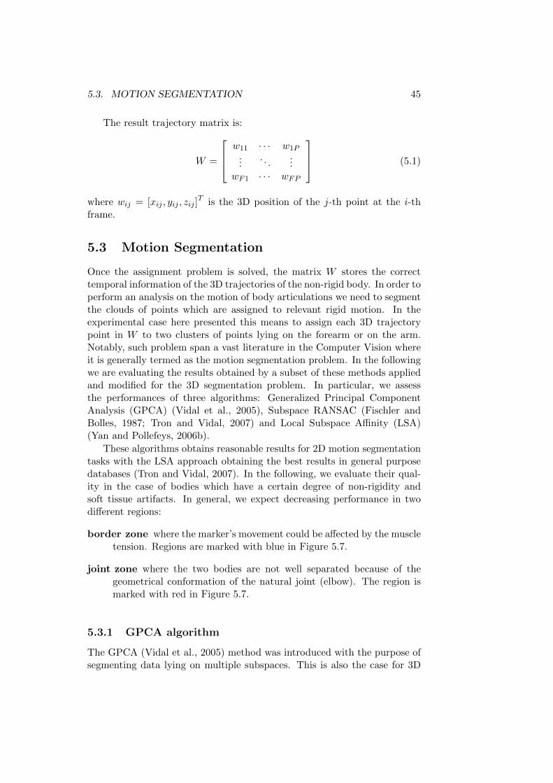
5.3. MOTION SEGMENTATION 45
The result trajectory matrix is:
W =
w11 · · · w1P...
. . ....
wF1 · · · wFP
(5.1)
where wij = [xij , yij , zij ]T is the 3D position of the j-th point at the i-th
frame.
5.3 Motion Segmentation
Once the assignment problem is solved, the matrix W stores the correcttemporal information of the 3D trajectories of the non-rigid body. In order toperform an analysis on the motion of body articulations we need to segmentthe clouds of points which are assigned to relevant rigid motion. In theexperimental case here presented this means to assign each 3D trajectorypoint in W to two clusters of points lying on the forearm or on the arm.Notably, such problem span a vast literature in the Computer Vision whereit is generally termed as the motion segmentation problem. In the followingwe are evaluating the results obtained by a subset of these methods appliedand modified for the 3D segmentation problem. In particular, we assessthe performances of three algorithms: Generalized Principal ComponentAnalysis (GPCA) (Vidal et al., 2005), Subspace RANSAC (Fischler andBolles, 1987; Tron and Vidal, 2007) and Local Subspace Affinity (LSA)(Yan and Pollefeys, 2006b).
These algorithms obtains reasonable results for 2D motion segmentationtasks with the LSA approach obtaining the best results in general purposedatabases (Tron and Vidal, 2007). In the following, we evaluate their qual-ity in the case of bodies which have a certain degree of non-rigidity andsoft tissue artifacts. In general, we expect decreasing performance in twodifferent regions:
border zone where the marker’s movement could be affected by the muscletension. Regions are marked with blue in Figure 5.7.
joint zone where the two bodies are not well separated because of thegeometrical conformation of the natural joint (elbow). The region ismarked with red in Figure 5.7.
5.3.1 GPCA algorithm
The GPCA (Vidal et al., 2005) method was introduced with the purpose ofsegmenting data lying on multiple subspaces. This is also the case for 3D
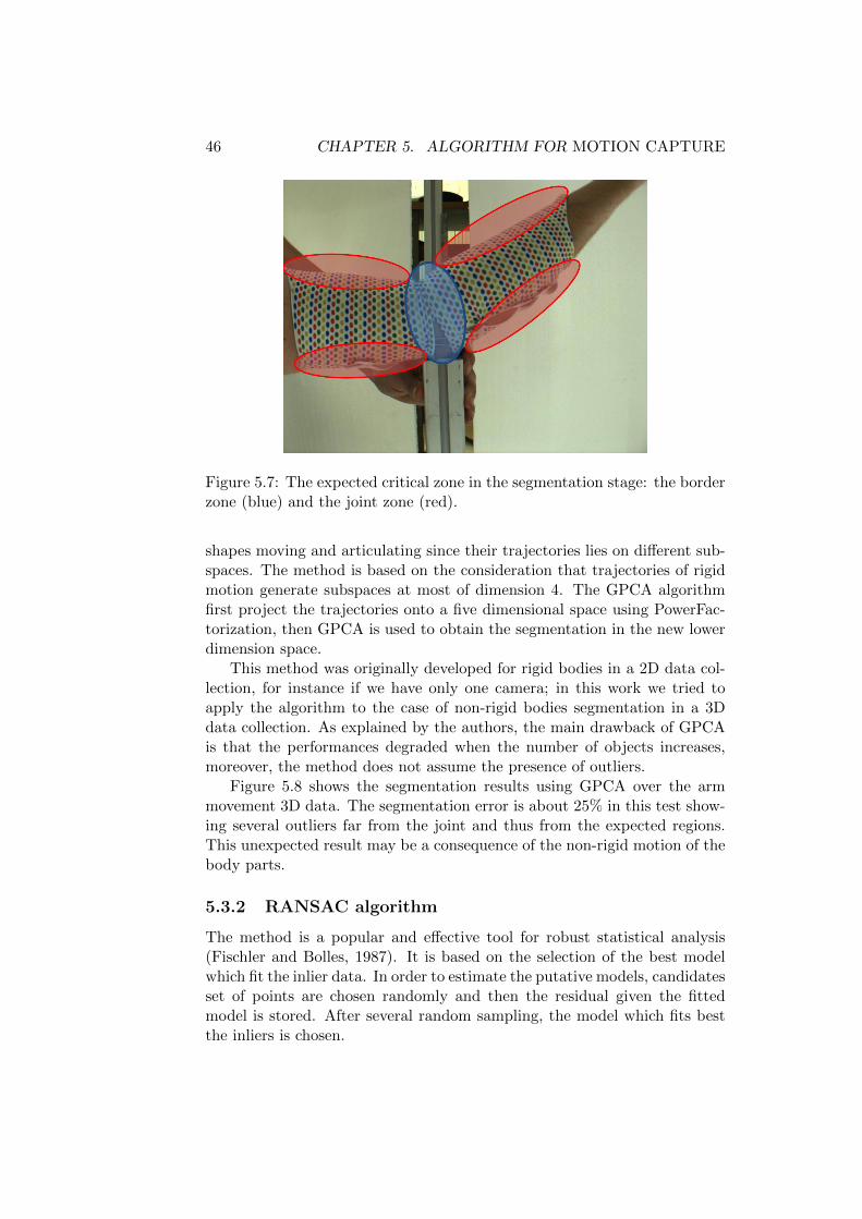
46 CHAPTER 5. ALGORITHM FOR MOTION CAPTURE
Figure 5.7: The expected critical zone in the segmentation stage: the borderzone (blue) and the joint zone (red).
shapes moving and articulating since their trajectories lies on different sub-spaces. The method is based on the consideration that trajectories of rigidmotion generate subspaces at most of dimension 4. The GPCA algorithmfirst project the trajectories onto a five dimensional space using PowerFac-torization, then GPCA is used to obtain the segmentation in the new lowerdimension space.
This method was originally developed for rigid bodies in a 2D data col-lection, for instance if we have only one camera; in this work we tried toapply the algorithm to the case of non-rigid bodies segmentation in a 3Ddata collection. As explained by the authors, the main drawback of GPCAis that the performances degraded when the number of objects increases,moreover, the method does not assume the presence of outliers.
Figure 5.8 shows the segmentation results using GPCA over the armmovement 3D data. The segmentation error is about 25% in this test show-ing several outliers far from the joint and thus from the expected regions.This unexpected result may be a consequence of the non-rigid motion of thebody parts.
5.3.2 RANSAC algorithm
The method is a popular and effective tool for robust statistical analysis(Fischler and Bolles, 1987). It is based on the selection of the best modelwhich fit the inlier data. In order to estimate the putative models, candidatesset of points are chosen randomly and then the residual given the fittedmodel is stored. After several random sampling, the model which fits bestthe inliers is chosen.
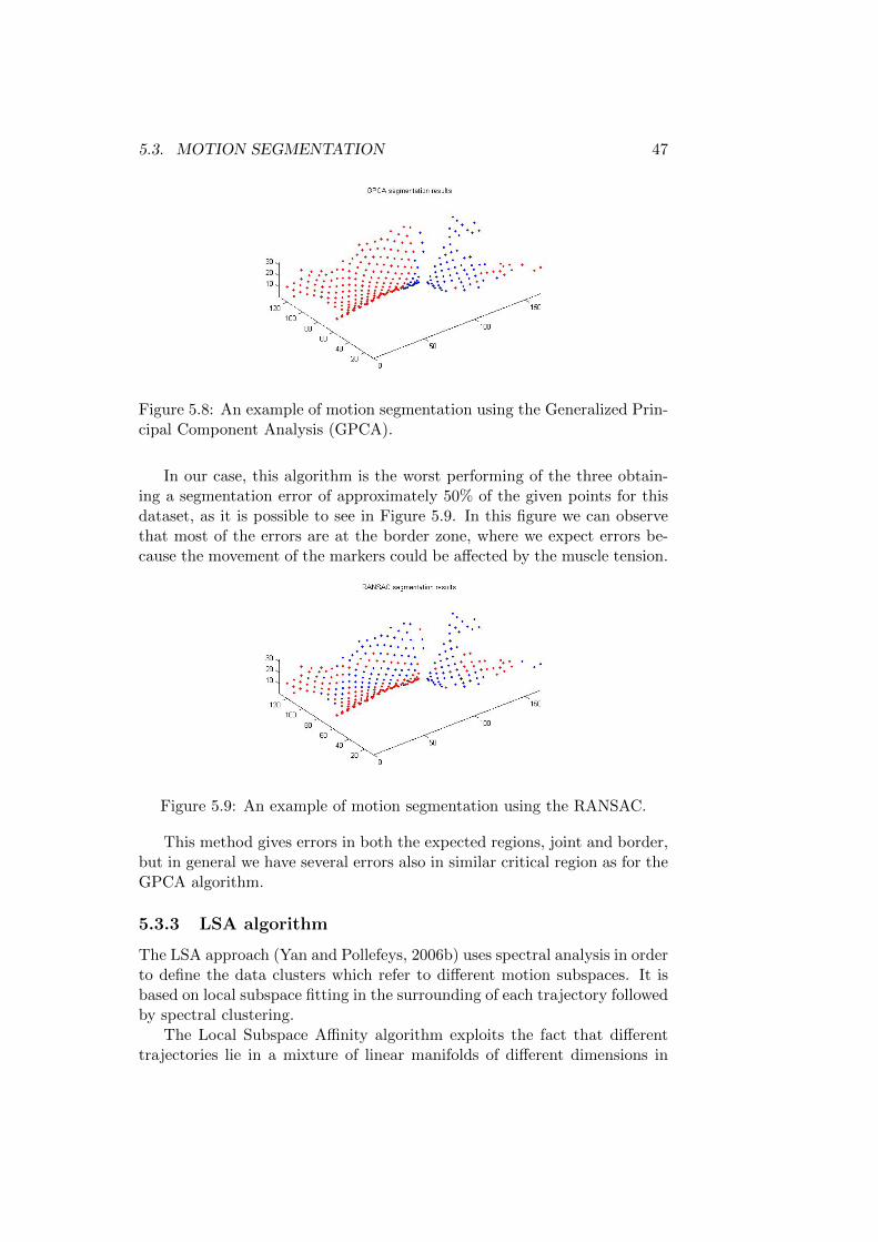
5.3. MOTION SEGMENTATION 47
Figure 5.8: An example of motion segmentation using the Generalized Prin-cipal Component Analysis (GPCA).
In our case, this algorithm is the worst performing of the three obtain-ing a segmentation error of approximately 50% of the given points for thisdataset, as it is possible to see in Figure 5.9. In this figure we can observethat most of the errors are at the border zone, where we expect errors be-cause the movement of the markers could be affected by the muscle tension.
Figure 5.9: An example of motion segmentation using the RANSAC.
This method gives errors in both the expected regions, joint and border,but in general we have several errors also in similar critical region as for theGPCA algorithm.
5.3.3 LSA algorithm
The LSA approach (Yan and Pollefeys, 2006b) uses spectral analysis in orderto define the data clusters which refer to different motion subspaces. It isbased on local subspace fitting in the surrounding of each trajectory followedby spectral clustering.
The Local Subspace Affinity algorithm exploits the fact that differenttrajectories lie in a mixture of linear manifolds of different dimensions in
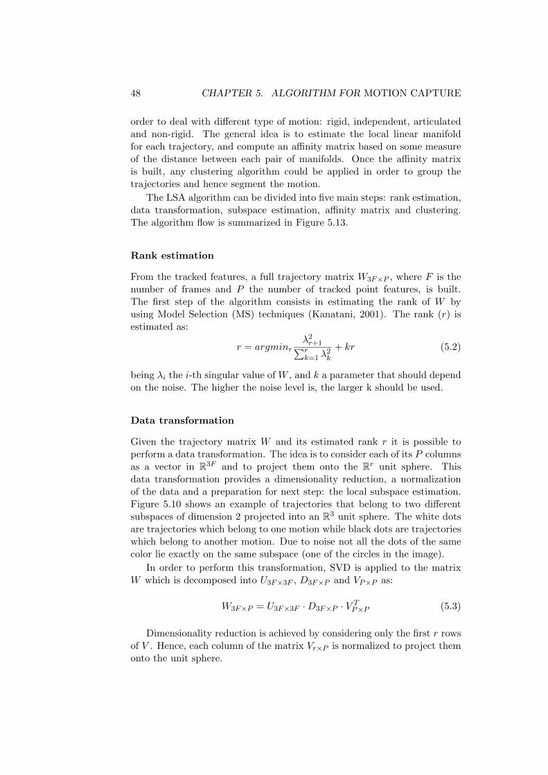
48 CHAPTER 5. ALGORITHM FOR MOTION CAPTURE
order to deal with different type of motion: rigid, independent, articulatedand non-rigid. The general idea is to estimate the local linear manifoldfor each trajectory, and compute an affinity matrix based on some measureof the distance between each pair of manifolds. Once the affinity matrixis built, any clustering algorithm could be applied in order to group thetrajectories and hence segment the motion.
The LSA algorithm can be divided into five main steps: rank estimation,data transformation, subspace estimation, affinity matrix and clustering.The algorithm flow is summarized in Figure 5.13.
Rank estimation
From the tracked features, a full trajectory matrix W3F×P , where F is thenumber of frames and P the number of tracked point features, is built.The first step of the algorithm consists in estimating the rank of W byusing Model Selection (MS) techniques (Kanatani, 2001). The rank (r) isestimated as:
r = argminrλ2r+1∑rk=1 λ
2k
+ kr (5.2)
being λi the i-th singular value of W , and k a parameter that should dependon the noise. The higher the noise level is, the larger k should be used.
Data transformation
Given the trajectory matrix W and its estimated rank r it is possible toperform a data transformation. The idea is to consider each of its P columnsas a vector in R3F and to project them onto the Rr unit sphere. Thisdata transformation provides a dimensionality reduction, a normalizationof the data and a preparation for next step: the local subspace estimation.Figure 5.10 shows an example of trajectories that belong to two differentsubspaces of dimension 2 projected into an R3 unit sphere. The white dotsare trajectories which belong to one motion while black dots are trajectorieswhich belong to another motion. Due to noise not all the dots of the samecolor lie exactly on the same subspace (one of the circles in the image).
In order to perform this transformation, SVD is applied to the matrixW which is decomposed into U3F×3F , D3F×P and VP×P as:
W3F×P = U3F×3F ·D3F×P · V TP×P (5.3)
Dimensionality reduction is achieved by considering only the first r rowsof V . Hence, each column of the matrix Vr×P is normalized to project themonto the unit sphere.
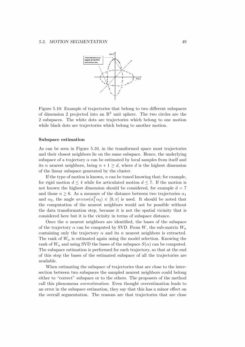
5.3. MOTION SEGMENTATION 49
Figure 5.10: Example of trajectories that belong to two different subspacesof dimension 2 projected into an R3 unit sphere. The two circles are the2 subspaces. The white dots are trajectories which belong to one motionwhile black dots are trajectories which belong to another motion.
Subspace estimation
As can be seen in Figure 5.10, in the transformed space most trajectoriesand their closest neighbors lie on the same subspace. Hence, the underlyingsubspace of a trajectory α can be estimated by local samples from itself andits n nearest neighbors, being n + 1 ≥ d, where d is the highest dimensionof the linear subspace generated by the cluster.
If the type of motion is known, n can be tuned knowing that; for example,for rigid motion d ≤ 4 while for articulated motion d ≤ 7. If the motion isnot known the highest dimension should be considered, for example d = 7and those n ≥ 6. As a measure of the distance between two trajectories α1
and α2, the angle arccos(αT1 α2) ∈ [0, π] is used. It should be noted thatthe computation of the nearest neighbors would not be possible withoutthe data transformation step, because it is not the spatial vicinity that isconsidered here but it is the vicinity in terms of subspace distance.
Once the n nearest neighbors are identified, the bases of the subspaceof the trajectory α can be computed by SVD. From W , the sub-matrix Wα
containing only the trajectory α and its n nearest neighbors is extracted.The rank of Wα is estimated again using the model selection. Knowing therank of Wα and using SVD the bases of the subspace S(α) can be computed.The subspace estimation is performed for each trajectory, so that at the endof this step the bases of the estimated subspace of all the trajectories areavailable.
When estimating the subspace of trajectories that are close to the inter-section between two subspaces the sampled nearest neighbors could belongeither to “correct” subspace or to the others. The proposers of the methodcall this phenomena overestimation. Even thought overestimation leads toan error in the subspace estimation, they say that this has a minor effect onthe overall segmentation. The reasons are that trajectories that are close
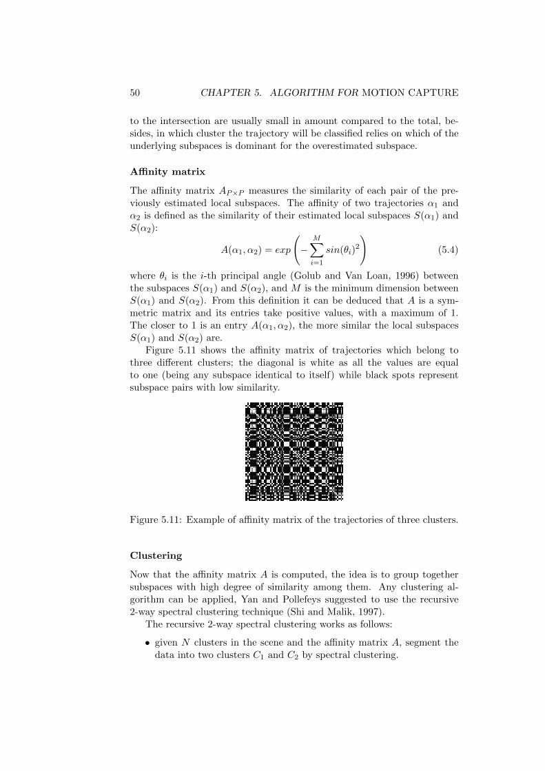
50 CHAPTER 5. ALGORITHM FOR MOTION CAPTURE
to the intersection are usually small in amount compared to the total, be-sides, in which cluster the trajectory will be classified relies on which of theunderlying subspaces is dominant for the overestimated subspace.
Affinity matrix
The affinity matrix AP×P measures the similarity of each pair of the pre-viously estimated local subspaces. The affinity of two trajectories α1 andα2 is defined as the similarity of their estimated local subspaces S(α1) andS(α2):
A(α1, α2) = exp
(−
M∑i=1
sin(θi)2
)(5.4)
where θi is the i-th principal angle (Golub and Van Loan, 1996) betweenthe subspaces S(α1) and S(α2), and M is the minimum dimension betweenS(α1) and S(α2). From this definition it can be deduced that A is a sym-metric matrix and its entries take positive values, with a maximum of 1.The closer to 1 is an entry A(α1, α2), the more similar the local subspacesS(α1) and S(α2) are.
Figure 5.11 shows the affinity matrix of trajectories which belong tothree different clusters; the diagonal is white as all the values are equalto one (being any subspace identical to itself) while black spots representsubspace pairs with low similarity.
Figure 5.11: Example of affinity matrix of the trajectories of three clusters.
Clustering
Now that the affinity matrix A is computed, the idea is to group togethersubspaces with high degree of similarity among them. Any clustering al-gorithm can be applied, Yan and Pollefeys suggested to use the recursive2-way spectral clustering technique (Shi and Malik, 1997).
The recursive 2-way spectral clustering works as follows:
• given N clusters in the scene and the affinity matrix A, segment thedata into two clusters C1 and C2 by spectral clustering.
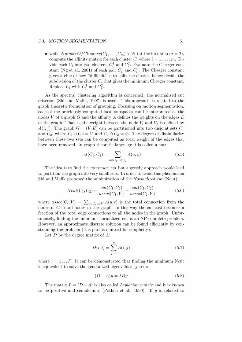
5.3. MOTION SEGMENTATION 51
• while NumberOfClusters(C1, . . . , Cm) < N (at the first step m = 2),compute the affinity matrix for each cluster Ci where i = 1, . . . ,m. Di-vide each Ci into two clusters, C1
i and C2i . Evaluate the Cheeger con-
stant (Ng et al., 2001) of each pair C1i and C2
i . The Cheeger constantgives a clue of how “difficult” is to split the cluster, hence decide thesubdivision of the cluster Cı that gives the minimum Cheeger constant.Replace Cı with C1
ı and C2ı .
As the spectral clustering algorithm is concerned, the normalized cutcriterion (Shi and Malik, 1997) is used. This approach is related to thegraph theoretic formulation of grouping. Focusing on motion segmentation,each of the previously computed local subspaces can be interpreted as thenodes V of a graph G and the affinity A defines the weights on the edges Eof the graph. That is, the weight between the node Vi and Vj is defined byA(i, j). The graph G = (V,E) can be partitioned into two disjoint sets C1
and C2, where C1 ∪ C2 = V and C1 ∩ C2 = . The degree of dissimilaritybetween these two sets can be computed as total weight of the edges thathave been removed. In graph theoretic language it is called a cut:
cut(C1, C2) =∑
u∈C1,v∈C2
A(u, v) (5.5)
The idea is to find the minimum cut but a greedy approach would leadto partition the graph into very small sets. In order to avoid this phenomenaShi and Malik proposed the minimization of the Normalized cut (Ncut):
Ncut(C1, C2) =cut(C1, C2)
assoc(C1, V )+
cut(C1, C2)
assoc(C2, V )(5.6)
where assoc(Ci, V ) =∑
u∈Ci,t∈V A(u, t) is the total connection from thenodes in Ci to all nodes in the graph. In this way the cut cost becomes afraction of the total edge connections to all the nodes in the graph. Unfor-tunately, finding the minimum normalized cut is an NP-complete problem.However, an approximate discrete solution can be found efficiently by con-straining the problem (this part is omitted for simplicity).
Let D be the degree matrix of A:
D(i, i) =
p∑j=1
A(i, j) (5.7)
where i = 1 . . . P . It can be demonstrated that finding the minimum Ncutis equivalent to solve the generalized eigenvalues system:
(D −A)y = λDy (5.8)
The matrix L = (D−A) is also called Laplacian matrix and it is knownto be positive and semidefinite (Pothen et al., 1990). If y is relaxed to
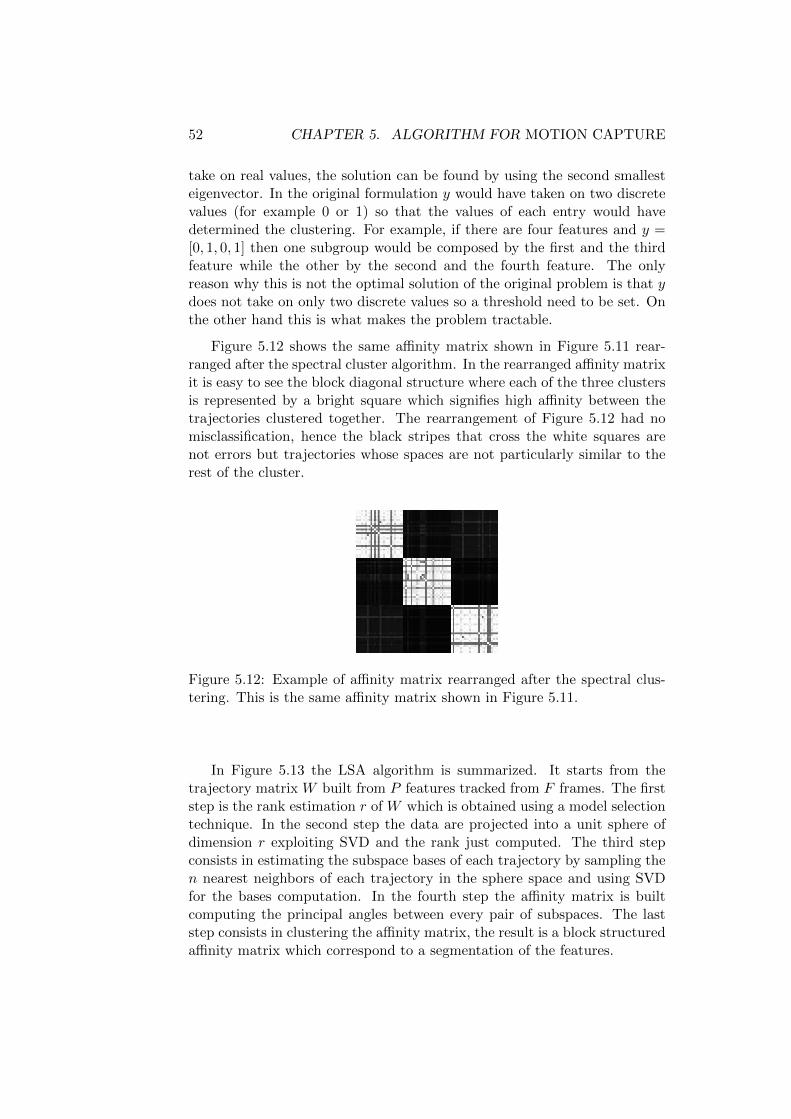
52 CHAPTER 5. ALGORITHM FOR MOTION CAPTURE
take on real values, the solution can be found by using the second smallesteigenvector. In the original formulation y would have taken on two discretevalues (for example 0 or 1) so that the values of each entry would havedetermined the clustering. For example, if there are four features and y =[0, 1, 0, 1] then one subgroup would be composed by the first and the thirdfeature while the other by the second and the fourth feature. The onlyreason why this is not the optimal solution of the original problem is that ydoes not take on only two discrete values so a threshold need to be set. Onthe other hand this is what makes the problem tractable.
Figure 5.12 shows the same affinity matrix shown in Figure 5.11 rear-ranged after the spectral cluster algorithm. In the rearranged affinity matrixit is easy to see the block diagonal structure where each of the three clustersis represented by a bright square which signifies high affinity between thetrajectories clustered together. The rearrangement of Figure 5.12 had nomisclassification, hence the black stripes that cross the white squares arenot errors but trajectories whose spaces are not particularly similar to therest of the cluster.
Figure 5.12: Example of affinity matrix rearranged after the spectral clus-tering. This is the same affinity matrix shown in Figure 5.11.
In Figure 5.13 the LSA algorithm is summarized. It starts from thetrajectory matrix W built from P features tracked from F frames. The firststep is the rank estimation r of W which is obtained using a model selectiontechnique. In the second step the data are projected into a unit sphere ofdimension r exploiting SVD and the rank just computed. The third stepconsists in estimating the subspace bases of each trajectory by sampling then nearest neighbors of each trajectory in the sphere space and using SVDfor the bases computation. In the fourth step the affinity matrix is builtcomputing the principal angles between every pair of subspaces. The laststep consists in clustering the affinity matrix, the result is a block structuredaffinity matrix which correspond to a segmentation of the features.
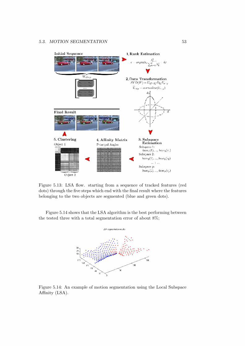
5.3. MOTION SEGMENTATION 53
Figure 5.13: LSA flow. starting from a sequence of tracked features (reddots) through the five steps which end with the final result where the featuresbelonging to the two objects are segmented (blue and green dots).
Figure 5.14 shows that the LSA algorithm is the best performing betweenthe tested three with a total segmentation error of about 8%;
Figure 5.14: An example of motion segmentation using the Local SubspaceAffinity (LSA).
54 CHAPTER 5. ALGORITHM FOR MOTION CAPTURE
The algorithm correctly estimate the points in the border zone, but wehave some (expected) errors in the joint zone. but the interesting thing isthat the mistakes out of the critical expected regions are very few. Thisis probably related to the fact that the LSA algorithm is more robust tothe noise possibly introduced by soft-tissue artifacts then the other twoconsidered approaches.
Because of the results shown in these preliminary tests, we propose touse LSA algorithm to segment the bodies.
5.4 Joint Reconstruction
Now that the points have been assigned to the respective body parts, itis now possible to compute the position and properties of the joint. Thetheoretical property used to perform the computation of the joint is thatthe subspaces computed from the trajectories of two body parts intersects.Such common intersection can be used to identify the joint position andproperties as noticed by (Yan and Pollefeys, 2008; Tresadern and Reid,2005) for image data and by (Fayad et al., 2009) for 3D data. We use thecomputational tool developed in the latter work to perform the estimationof the joint values.
This method is composed of three steps:
1. we refine a factorization method for Structure from Motion (SfM) byapplying a variation of the weighted PCT, based on least-squares opti-mization; so that we have a first rigid approximation for each segmentof the non-rigid bodies.
2. we use a quadratic model for non-rigid bodies, initialized by the firstestimate of the rigid segment, to compute a more accurate rigid com-ponent of the non-rigid segments.
3. we combine the techniques for articulated SfM and our model for thenon-rigid segments, to provide a final 3D articulated model of thehuman body.
5.4.1 Factorization method
Factorization methods for Structure from Motion are a family of image basedalgorithms that model moving objects as a product of two factors: motionand shape. The shape parameters are defined as the 3D geometric proper-ties of the object; the motion parameters are defined as the time-varyingparameters of the motion (e.g. rotations and translations of the rigid body)that the shape performs in a metric space.
The factorization method proposed by Fayad (Fayad, 2008) assumes aset of P 3D feature points being tracked over F frames. The method relies
5.4. JOINT RECONSTRUCTION 55
on the key fact that 3D trajectories of points belonging to the same bodyshare the same global properties.
From the Section 5.2, we have a matrixW that represents the trajectoriesof all the feature points as:
W =
w11 · · · w1P...
. . ....
wF1 · · · wFP
(5.9)
where wij ∈ R3 is a 3 elements column vector that contains the 3D co-ordinates of point j at frame i. Each 3D point wij can be written, inhomogeneous coordinates, as:
wij = [Ri|ti][sj1
](5.10)
where sj = [xj , yj , zj ]T are the coordinates of the point j on a local reference
frame, and Mi and ti are respectively the rotation matrix and the translationvector that describe sj with respect to a global reference frame. Stackingthese equations for all the F frames and P points, we have:
W =
W1...
WF
=
M1...
MF
[ S1 · · · Sp]
+
T1...TF
= MS + T (5.11)
where Ti = [ti, 1TP ], with 1TP being a vector of P elements with all entries
equal to 1. The translational component ti can be computed as the coor-dinates of the centroid of the point cloud at each frame Wi. Thus, it canbe easily eliminated by registering, at each frame, the point cloud to theorigin i.e at each frame we subtract to the coordinates of every point themean of the point cloud coordinates. In this scenario, it frequently occursthat, instead of W , we consider a registered form of this matrix i.e. we usea matrix W such that:
W = W − T = MS (5.12)
In this equation M is a < 3F × r > matrix and S a < r × P > matrix,where r is the rank of the matrix W and it depends by the type of shapeconsidered.
Rigid bodies
A rigid body moving rigidly brings the dimensionality of the bilinear modelsto either r ≤ 3, if we consider the registered trajectory matrix, or r ≤ 4 ifwe consider the translation vector too. Given this rank constraint, and
56 CHAPTER 5. ALGORITHM FOR MOTION CAPTURE
remembering the equation 5.12, we can compute a factorization of W byperforming a Singular Value Decomposition (SVD) giving:
W = MS = UrΣrVTr (5.13)
where Ur is a 3F × r orthogonal matrix, Σr a r × r diagonal matrix and Vra P × r orthogonal matrix. This initial decomposition via SVD can providea first affine fit of the motion and shape components M and S such that:
M = UrΣ1/2r and S = Σ1/2
r V Tr (5.14)
The initial factorization proposed in equation 5.14 do not guarantee thatM is in fact a collection of F 3 × 3 rotation matrices. Since this transfor-mation is valid up to an affine transformation i.e. W = MQQ−1S we seek aspecific transformation Q which enforces the metric properties of M . Thiscan be achieved by imposing orthogonality constraints on MiQ, which isdone by solving the set of linear equations for all the F frames:
mTikHmik = 1
mTikHmil = 0, ∀l 6= k (5.15)
with k, l = 1, 2, 3, mik and mil are respectively the k-th and l-th row ofmatrix Mi, and H = QQT is symmetric matrix (as Q is upper triangular).Q can thus be recovered from H by using Cholesky decomposition. Weupdate the factorization in equation 5.14 to:
M = MQ and S = Q−1S (5.16)
When the scene is composed of N rigid objects moving independently,the same considerations are valid. The model is simply expanded for each ofthe different independent objects, with S showing a block diagonal structure:
W =[M1 · · · MN
] S1
. . .
SN
(5.17)
In this case the rank condition becomes r ≤ 3N .
Articulated bodies
However if the rigid objects are linked by joints their motions are not inde-pendent and there is a loss in the degrees of freedom of the system. Thisconstraint on the movement manifests itself in the measurement matrix Was a decrease in rank (Tresadern and Reid, 2005; Yan and Pollefeys, 2006a).For the sake of simplicity we will only consider systems of two rigid bodies
5.4. JOINT RECONSTRUCTION 57
linked by a joint, two types of joints are here considered: the universal jointand the hinge joint.
Universal joint
By universal (spherical) joint we mean a kind of joint in which eachbody is at a fixed distance to the joint center, being the relative position ofthe bodies constrained, but their rotations remaining independent. At eachframe the shapes connected by a joint satisfy the following relation:
R1d1 + t1 = −R2d2 + t2 (5.18)
where t1 and t2 are the 3D shape centroids of the two objects, R1 and R2
the 3 × 3 rotation matrices and d1 and d2 the 3D displacement vectors ofeach shape from the central joint.
Thus we can write t2 as a function of t1, and we are now able to factorizethe trajectory matrix as:
W = [W1|W2] = [R1 R2 t1]
S1 d1
0 S2 + d2
1 1
(5.19)
where W1 and W2 are respectively the measurement matrices for the firstand second body.
By using the equation 5.18 the joint parameters d1 and d2 are easilycomputed once we have found the motion parameters R1, R2, t1 and t2.
After the registration of each body to the origin of the global referenceframe, the registered trajectory matrix W is a 3F × (P1 + P2) matrix withrank 6, and so:
W = [R1|R2]
[S1 00 S2
](5.20)
Now we can perform the truncated SVD with k = 6.
W = UkΣkVTk = [U1|U2]3F×6[V1|V2]6×(P1+P2) (5.21)
However the factorization is not final as [V1|V2] is a dense matrix. If wedefine an operator Nl(·) that returns the left null-space of its argument, wecan define a 6× 6 transformation matrix TU such that:
TU =
[Nl(V2)Nl(V1)
](5.22)
We can now recover S by pre-multiplying it by TU :
S =
[Nl(V2)Nl(V1)
][V1|V2] =
[Nl(V2)V1 Nl(V2)V2
Nl(V1)V1 Nl(V1)V2
]=
[S1 00 S2
](5.23)

58 CHAPTER 5. ALGORITHM FOR MOTION CAPTURE
As we must keep the original data unaltered, we have to post-multiply[U1|U2] by T−1
U :
M = [U1|U2]
[Nl(V2)Nl(V1)
]−1
= [M1|M2] (5.24)
Hinge JointIn a hinge joint, two bodies can rotate around an axis such that the
distance to that rotation axis is constant. Therefore their rotation matricesR1 and R2 are not completely independent.
From the geometry of the joint, we can see that every vector belongingto any of the two bodies, that is parallel to the joint axis, must remainso throughout the movement. Without loss of generality, we can choose alocal reference frame with x-axis coincident with the axis of rotation of thejoint. Let ex = [1 0 0]T be the x-axis unit vector. Applying a general 3× 3rotation matrix R = [c1 c2 c3] to ex will result in c1 · ex, the only column ofthe rotation matrix that affects vectors parallel to the x-axis is the first one.Therefore, to comply with the joint constraints, the first column of R1 mustbe equal to the first column of R2. We can now define the rotation matricesas R1 = [c1 c2 c3] and R2 = [c1 c4 c5]. As all the points belonging to therotation axis must fulfill both movement conditions, thus, when consideringregistered data, W will then be given by:
W = [c1 c2 c3 c4 c5]
x1
1 · · · x(1)P1
x(2)1 · · · x
(2)P2
y11 · · · y
(1)P1
0 · · · 0
z11 · · · z
(1)P1
0 · · · 0
0 · · · 0 y(2)1 · · · y
(2)P2
0 · · · 0 z(2)1 · · · z
(2)P2
(5.25)
Once again we use the truncated SVD of W as the first step on theparameter estimation. In this case we use k = 5 giving:
W = UkΣkVTk = [U1|U2]3F×5[V1|V2]5×(P1+P2) (5.26)
As we have seen when we spoke about universal joints, this matrix [V1|V2]is a dense matrix, but what we need is to compute a matrix S with thestructure defined in equation 5.25. Let TH be a transformation matrix suchthat:
TH =
bT
Nl(V2)Nl(V1)
(5.27)
whereNl(·) is the operator that returns the left null-space of its argument (asdefined previously), and bT = [1 0 0 0 0 0]. By pre-multiplying [V1|V2] with
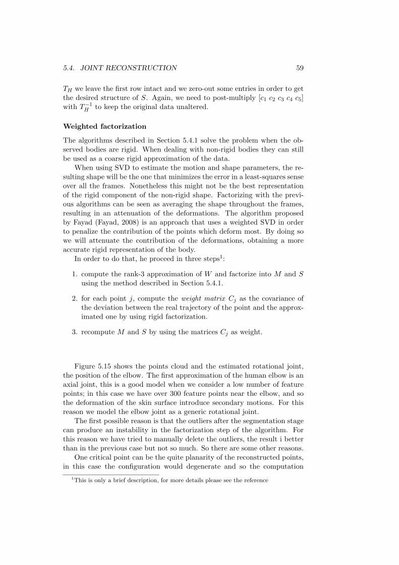
5.4. JOINT RECONSTRUCTION 59
TH we leave the first row intact and we zero-out some entries in order to getthe desired structure of S. Again, we need to post-multiply [c1 c2 c3 c4 c5]with T−1
H to keep the original data unaltered.
Weighted factorization
The algorithms described in Section 5.4.1 solve the problem when the ob-served bodies are rigid. When dealing with non-rigid bodies they can stillbe used as a coarse rigid approximation of the data.
When using SVD to estimate the motion and shape parameters, the re-sulting shape will be the one that minimizes the error in a least-squares senseover all the frames. Nonetheless this might not be the best representationof the rigid component of the non-rigid shape. Factorizing with the previ-ous algorithms can be seen as averaging the shape throughout the frames,resulting in an attenuation of the deformations. The algorithm proposedby Fayad (Fayad, 2008) is an approach that uses a weighted SVD in orderto penalize the contribution of the points which deform most. By doing sowe will attenuate the contribution of the deformations, obtaining a moreaccurate rigid representation of the body.
In order to do that, he proceed in three steps1:
1. compute the rank-3 approximation of W and factorize into M and Susing the method described in Section 5.4.1.
2. for each point j, compute the weight matrix Cj as the covariance ofthe deviation between the real trajectory of the point and the approx-imated one by using rigid factorization.
3. recompute M and S by using the matrices Cj as weight.
Figure 5.15 shows the points cloud and the estimated rotational joint,the position of the elbow. The first approximation of the human elbow is anaxial joint, this is a good model when we consider a low number of featurepoints; in this case we have over 300 feature points near the elbow, and sothe deformation of the skin surface introduce secondary motions. For thisreason we model the elbow joint as a generic rotational joint.
The first possible reason is that the outliers after the segmentation stagecan produce an instability in the factorization step of the algorithm. Forthis reason we have tried to manually delete the outliers, the result i betterthan in the previous case but not so much. So there are some other reasons.
One critical point can be the quite planarity of the reconstructed points,in this case the configuration would degenerate and so the computation
1This is only a brief description, for more details please see the reference
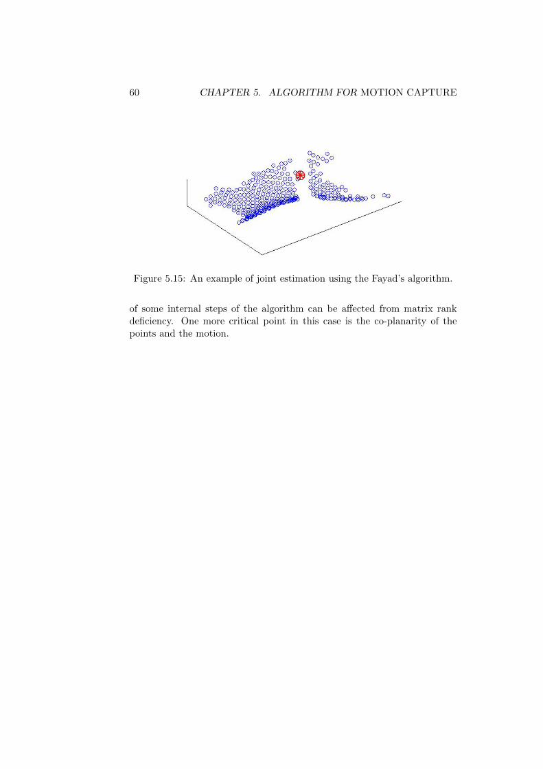
60 CHAPTER 5. ALGORITHM FOR MOTION CAPTURE
Figure 5.15: An example of joint estimation using the Fayad’s algorithm.
of some internal steps of the algorithm can be affected from matrix rankdeficiency. One more critical point in this case is the co-planarity of thepoints and the motion.

Part III
Experimental section
61

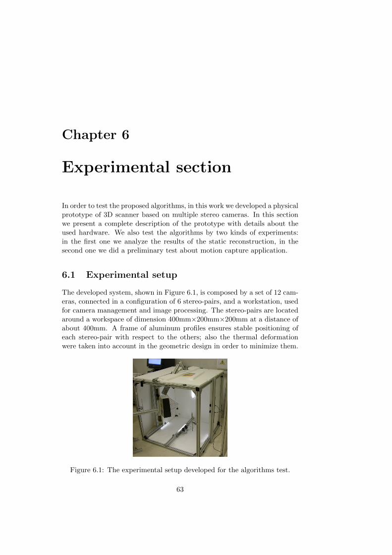
Chapter 6
Experimental section
In order to test the proposed algorithms, in this work we developed a physicalprototype of 3D scanner based on multiple stereo cameras. In this sectionwe present a complete description of the prototype with details about theused hardware. We also test the algorithms by two kinds of experiments:in the first one we analyze the results of the static reconstruction, in thesecond one we did a preliminary test about motion capture application.
6.1 Experimental setup
The developed system, shown in Figure 6.1, is composed by a set of 12 cam-eras, connected in a configuration of 6 stereo-pairs, and a workstation, usedfor camera management and image processing. The stereo-pairs are locatedaround a workspace of dimension 400mm×200mm×200mm at a distance ofabout 400mm. A frame of aluminum profiles ensures stable positioning ofeach stereo-pair with respect to the others; also the thermal deformationwere taken into account in the geometric design in order to minimize them.
Figure 6.1: The experimental setup developed for the algorithms test.
63
64 CHAPTER 6. EXPERIMENTAL SECTION
Each stereo-pair is composed from two Point Grey Chamaleon USB cam-eras (Point Grey Research, Inc., 2009), with CMOS RGB sensor with max-imal resolution of 1280×960 pixels. The two cameras are stuck on an ironbar, and then connected to the structure. The cameras are all triggeredin order to ensure that all the images are acquired simultaneously. Thelenses are standard C-mount lenses with focal length 6mm and f-number1.4; this ensure a field of view of about 400mm×300mm at a distance ofabout 400mm. With reference to Figure 6.2, the baseline (b) is set at about140mm, in order to have a compromise between accuracy in triangulationand common marker detection (Brown et al., 2003). The angle betweenthe optical axis of two cameras is computed in order to have the maximaloverlapping between the two fields of view at a distance (d) of 400mm; inthis case the angle (α) is about 15.
Figure 6.2: The angle between cameras in a stereo-pair. In the developedprototype α ∼= 15.
A system of LED lightning and diffusive polystyrene panels is used inorder to have in the workspace the light as most diffuse as possible.
We wrote a software for camera management and synchronous imageacquisition. The software provides the following tasks:
• recognizes all the cameras connected to the PC by ID-number
• switch on and initializes all the cameras
• set camera parameters as described in a configuration file
• acquires synchronous images from all the connected cameras
• save the images in folders and files, according to ID-number of eachcamera and a look-up table.
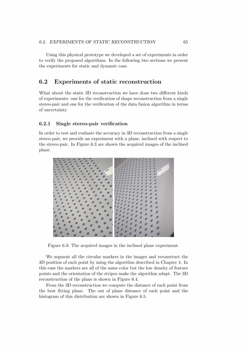
6.2. EXPERIMENTS OF STATIC RECONSTRUCTION 65
Using this physical prototype we developed a set of experiments in orderto verify the proposed algorithms. In the following two sections we presentthe experiments for static and dynamic case.
6.2 Experiments of static reconstruction
What about the static 3D reconstruction we have done two different kindsof experiments: one for the verification of shape reconstruction from a singlestereo-pair and one for the verification of the data fusion algorithm in termsof uncertainty.
6.2.1 Single stereo-pair verification
In order to test and evaluate the accuracy in 3D reconstruction from a singlestereo-pair, we provide an experiment with a plane, inclined with respect tothe stereo-pair. In Figure 6.3 are shown the acquired images of the inclinedplane.
Figure 6.3: The acquired images in the inclined plane experiment.
We segment all the circular markers in the images and reconstruct the3D position of each point by using the algorithm described in Chapter 4. Inthis case the markers are all of the same color but the low density of featurepoints and the orientation of the stripes make the algorithm adapt. The 3Dreconstruction of the plane is shown in Figure 6.4.
From the 3D reconstruction we compute the distance of each point fromthe best fitting plane. The out of plane distance of each point and thehistogram of this distribution are shown in Figure 6.5.
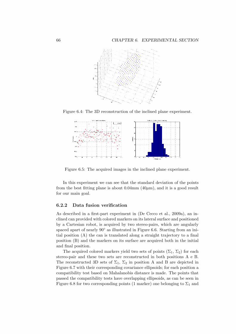
66 CHAPTER 6. EXPERIMENTAL SECTION
Figure 6.4: The 3D reconstruction of the inclined plane experiment.
Figure 6.5: The acquired images in the inclined plane experiment.
In this experiment we can see that the standard deviation of the pointsfrom the best fitting plane is about 0.04mm (40µm), and it is a good resultfor our main goal.
6.2.2 Data fusion verification
As described in a first-part experiment in (De Cecco et al., 2009a), an in-clined can provided with colored markers on its lateral surface and positionedby a Cartesian robot, is acquired by two stereo-pairs, which are angularlyspaced apart of nearly 90 as illustrated in Figure 6.6. Starting from an ini-tial position (A) the can is translated along a straight trajectory to a finalposition (B) and the markers on its surface are acquired both in the initialand final position.
The acquired colored markers yield two sets of points (Σ1, Σ2) for eachstereo-pair and these two sets are reconstructed in both positions A e B.The reconstructed 3D sets of Σ1, Σ2 in position A and B are depicted inFigure 6.7 with their corresponding covariance ellipsoids; for each position acompatibility test based on Mahalanobis distance is made. The points thatpassed the compatibility tests have overlapping ellipsoids, as can be seen inFigure 6.8 for two corresponding points (1 marker) one belonging to Σ1 and
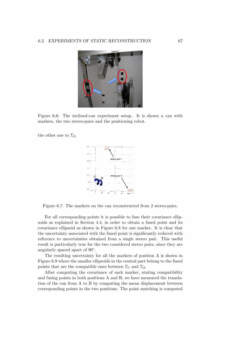
6.2. EXPERIMENTS OF STATIC RECONSTRUCTION 67
Figure 6.6: The inclined-can experiment setup. It is shown a can withmarkers, the two stereo-pairs and the positioning robot.
the other one to Σ2.
Figure 6.7: The markers on the can reconstructed from 2 stereo-pairs.
For all corresponding points it is possible to fuse their covariance ellip-soids as explained in Section 4.4, in order to obtain a fused point and itscovariance ellipsoid as shown in Figure 6.8 for one marker. It is clear thatthe uncertainty associated with the fused point is significantly reduced withreference to uncertainties obtained from a single stereo pair. This usefulresult is particularly true for the two considered stereo pairs, since they areangularly spaced apart of 90.
The resulting uncertainty for all the markers of position A is shown inFigure 6.9 where the smaller ellipsoids in the central part belong to the fusedpoints that are the compatible ones between Σ1 and Σ2.
After computing the covariance of each marker, stating compatibilityand fusing points in both positions A and B, we have measured the transla-tion of the can from A to B by computing the mean displacement betweencorresponding points in the two positions. The point matching is computed
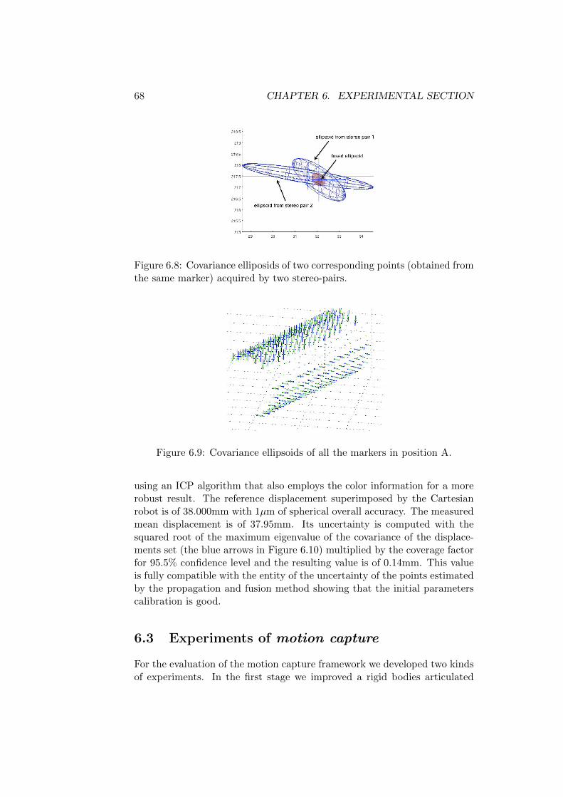
68 CHAPTER 6. EXPERIMENTAL SECTION
Figure 6.8: Covariance elliposids of two corresponding points (obtained fromthe same marker) acquired by two stereo-pairs.
Figure 6.9: Covariance ellipsoids of all the markers in position A.
using an ICP algorithm that also employs the color information for a morerobust result. The reference displacement superimposed by the Cartesianrobot is of 38.000mm with 1µm of spherical overall accuracy. The measuredmean displacement is of 37.95mm. Its uncertainty is computed with thesquared root of the maximum eigenvalue of the covariance of the displace-ments set (the blue arrows in Figure 6.10) multiplied by the coverage factorfor 95.5% confidence level and the resulting value is of 0.14mm. This valueis fully compatible with the entity of the uncertainty of the points estimatedby the propagation and fusion method showing that the initial parameterscalibration is good.
6.3 Experiments of motion capture
For the evaluation of the motion capture framework we developed two kindsof experiments. In the first stage we improved a rigid bodies articulated
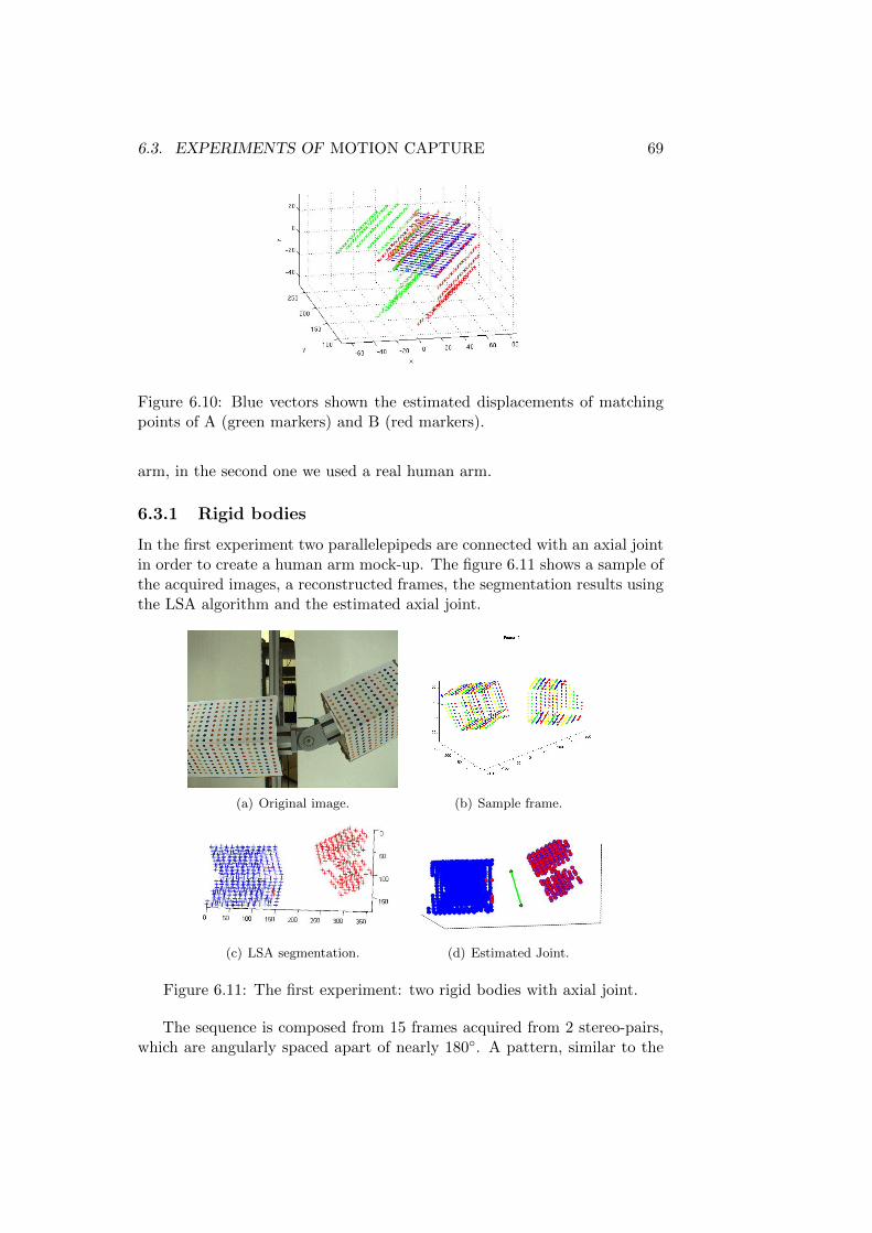
6.3. EXPERIMENTS OF MOTION CAPTURE 69
Figure 6.10: Blue vectors shown the estimated displacements of matchingpoints of A (green markers) and B (red markers).
arm, in the second one we used a real human arm.
6.3.1 Rigid bodies
In the first experiment two parallelepipeds are connected with an axial jointin order to create a human arm mock-up. The figure 6.11 shows a sample ofthe acquired images, a reconstructed frames, the segmentation results usingthe LSA algorithm and the estimated axial joint.
(a) Original image. (b) Sample frame.
(c) LSA segmentation. (d) Estimated Joint.
Figure 6.11: The first experiment: two rigid bodies with axial joint.
The sequence is composed from 15 frames acquired from 2 stereo-pairs,which are angularly spaced apart of nearly 180. A pattern, similar to the
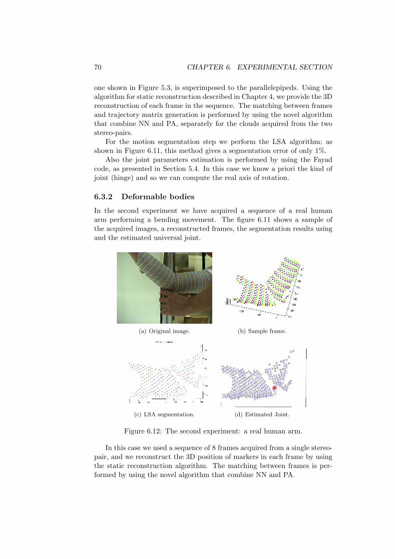
70 CHAPTER 6. EXPERIMENTAL SECTION
one shown in Figure 5.3, is superimposed to the parallelepipeds. Using thealgorithm for static reconstruction described in Chapter 4, we provide the 3Dreconstruction of each frame in the sequence. The matching between framesand trajectory matrix generation is performed by using the novel algorithmthat combine NN and PA, separately for the clouds acquired from the twostereo-pairs.
For the motion segmentation step we perform the LSA algorithm; asshown in Figure 6.11, this method gives a segmentation error of only 1%.
Also the joint parameters estimation is performed by using the Fayadcode, as presented in Section 5.4. In this case we know a priori the kind ofjoint (hinge) and so we can compute the real axis of rotation.
6.3.2 Deformable bodies
In the second experiment we have acquired a sequence of a real humanarm performing a bending movement. The figure 6.11 shows a sample ofthe acquired images, a reconstructed frames, the segmentation results usingand the estimated universal joint.
(a) Original image. (b) Sample frame.
(c) LSA segmentation. (d) Estimated Joint.
Figure 6.12: The second experiment: a real human arm.
In this case we used a sequence of 8 frames acquired from a single stereo-pair, and we reconstruct the 3D position of markers in each frame by usingthe static reconstruction algorithm. The matching between frames is per-formed by using the novel algorithm that combine NN and PA.

6.3. EXPERIMENTS OF MOTION CAPTURE 71
In this experiments the total segmentation error using LSA algorithm isof about 8%. The first approximation of the human elbow doing a bendingmovement is an axial joint; nevertheless we have two conditions that disturbthis approximation: the high number of feature points and the skin-bonesinternal movement and muscolar deformations. For this reason we modelthe elbow joint as a generic rotational joint (universal).
In this configuration, the joint reconstruction has two critical points:
• the outliers after the segmentation stage can produce an instability inthe factorization step of the algorithm.
• the co-planarity of the points and the motion. If the point cloud isquite planar the configuration would degenerate and so the compu-tation of some internal steps of the algorithm can be affected frommatrix rank deficiency.

72 CHAPTER 6. EXPERIMENTAL SECTION
Chapter 7
Conclusions
In this work we presented a set of algorithms for 3D shapes reconstruc-tion and motion segmentation for the application to multiple stereo-camerasystem and deformable bodies. In particular we were interested in the ap-plication to human body analysis.
In the first part of the work, we presented a complete framework for3D static scanning, based on a multiple stereo vision approach. The frame-work provides the 3D reconstruction of a set of markers belonging to thesurface of a target body; the 3D position of each marker is computed fromeach stereo-pair by using the triangulation algorithm. Later the position ofpoints viewed from more than one pair are fused performing a compatibilityanalysis based on uncertainty ellipsoids of each point.
An extension to the motion analysis is presented in the second part ofthe work. We describe here a complete framework for the points matchingamong a sequence of frames, the segmentation of the bodies based on themotion analysis, and the identification of the joint parameters. This algo-rithm is oriented to the application to a collection of 3D data of non-rigidbodies.
A prototype of 3D scanner was developed at the Mechatronics Labora-tory at the University of Trento and the presented algorithm were testedin an experimental section that comprises the analysis of static reconstruc-tion, of planar and cylindrical surfaces, and motion analysis, of rigid andnon-rigid jointed bodies.
This work represents a solid basis for the realization of a 3D scannerbased on vision technologies. All the algorithm developed are implementedas modular software, this will intervene and improve on individual parts. Inparticular some points to improve are:
• replace the colored circular markers with natural features, this can bedone modifying only the marker detection and feature matching algo-rithms, and developing a new method for the estimation of uncertainty
73

74 CHAPTER 7. CONCLUSIONS
in feature detection.
• replace the multiple stereo approach with the multiple camera one,this can be done modifying the triangulation algorithm and, slightly,the uncertainty propagation one. Notice that in this case there is nolonger needed of compatibility analysis and points fusion stages.
Most of the work has been supported by Delta R&S Company and partof the algorithms was implemented in their products.
The work here presented resulted in two congress paper (De Cecco et al.,2009a; De Cecco et al., 2009c), a journal paper (De Cecco et al., 2009b) anda submitted congress paper.
Bibliography
Amat, J., Frigola, M., and Casals, A. (2002). Selection of the best stereo pairin a multi-camera configuration. In Proceedings of the IEEE Interna-tional Conference on Robotics and Automation (ICRA 2002), volume 4,pages 3342–3346.
Barnard, R. W., Pearce, K., and Schovanec, L. (2001). Inequalities for theperimeter of an ellipse. Journal of Mathematical Analysis and Applica-tions, 260(2):295–306.
BIPM, IEC, IFCC, ISO, IUPAP, and OIML (1993). Guide to the Expressionof Uncertainty in Measurement. ISO - International Organization forStandardization.
Born, M. and Wolf, E. (1999). Principles of Optics: Electromagnetic The-ory of Propagation, Interference and Diffraction of Light. CambridgeUniversity Press, 7th edition.
Boujou (2009). Boujou. http://www.vicon.com/boujou/.
Brown, M. Z., Burschka, D., and Hager, G. D. (2003). Advances in compu-tational stereo. IEEE Transactions on Pattern Analysis and MachineIntelligence, 25:993–1008.
Canny, J. F. (1986). A computational approach to edge detection. IEEETransactions on Pattern Analysis and Machine Intelligence, 8(6):679–698.
Celenk, M. and Bachnak, R. (1990). Multiple stereo vision for 3d objectreconstruction. In IEEE International Conference on Systems Engi-neering, pages 555–558.
Chen, J., Ding, Z., and Yuan, F. (2008). Theoretical uncertainty evalu-ation of stereo reconstruction. In The 2nd International Conferenceon Bioinformatics and Biomedical Engineering (ICBBE 2008), pages2378–2381.
75

76 BIBLIOGRAPHY
Corazza, S., Mundermann, L., and Andriacchi, T. (2007). A frameworkfor the functional identification of joint centers using markerless mo-tion capture, validation for the hip joint. Journal of Biomechanics,40(15):3510–3515.
De Cecco, M., Baglivo, L., Parzianello, G., Lunardelli, M., Setti, F., andPertile, M. (2009a). Uncertainty analysis for multi-stereo 3d shapeestimation. In IEEE International Workshop on Advanced Methodsfor Uncertainty Estimation in Measurement, pages 22–27, Bucharest,Romania.
De Cecco, M., Pertile, M., Baglivo, L., Lunardelli, M., Setti, F., and Tav-ernini, M. (2009b). A unified framework for uncertainty, compatibilityanalysis and data fusion for multi-stereo 3d shape estimation. IEEETransactions on Instrumentation Measurements. Accepted for publica-tion.
De Cecco, M., Pertile, M., Baglivo, L., Parzianello, G., Lunardelli, M., Setti,F., and Selmo, A. (2009c). Multi-stereo compatibility analysis for 3dshape estimation. In XIX IMEKO World Congress, Fundamental andApplied Metrology, pages 1909–1914, Lisbon, Portugal.
Devernay, F. and Faugeras, O. (2001). Straight lines have to be straight: au-tomatic calibration and removal of distortion from scenes of structuredenviroments. Machine Vision Applications, 13(1):14–24.
Duda, R. O., Hart, P. E., and Stork, D. (2000). Pattern Classification.Wiley-Interscience Publication.
Eggert, D. W., Lorusso, A., and Fisher, R. B. (1997). Estimating 3-d rigidbody transformations: a comparison of four major algorithms. MachineVision Application, 9(5-6):272–290.
Fayad, J., Del Bue, A., Agapito, L., and Aguiar, P. (2009). Human bodymodeling using quadratic deformations. In 7th EUROMECH Solid Me-chanics Conference, Lisbon, Portugal.
Fayad, J. R. K. (2008). Articulated three-dimensional human modeling frommotion capture systems. Master’s thesis, Instituto Superior Tecnico,Universidade Tecnica de Lisboa.
Fischler, M. and Bolles, R. (1987). Random sample consensus: A paradigmfor model fitting with applications to image analysis and automatedcartography. In Fischler, M. A. and Firschein, O., editors, Readings inComputer Vision: Issues, Problems, Principles, and Paradigms, pages726–740. Los Altos, CA.
BIBLIOGRAPHY 77
Forsyth, D. A. and Ponce, J. (2002). Computer Vision: A Modern Approach.Prentice Hall.
Goldstein, H., Poole, C. P., and Safko, J. L. (2001). Classical Mechanics.Addison Wesley, 3rd edition.
Golub, G. H. and Van Loan, C. F. (1996). Matrix Computations. The JohnsHopkins University Press, Baltimore, MD (USA), 3rd edition.
Hartley, R. I. and Zisserman, A. (2004). Multiple View Geometry in Com-puter Vision. Cambridge University Press, second edition.
Hernandez Esteban, C. and Schmitt, F. (2002). Multi-stereo 3d object re-construction. In Proceedings of the First International Symposium on3D Data Processing Visualization and Transmission, pages 159–166.
Horn, B. K. P. (2000). Tsai’s camera calibration method revisited. http:
//people.csail.mit.edu/bkph/articles/Tsai_Revisited.pdf.
Ioannidis, D., Tzovaras, D., Damousis, I. G., Argyropoulos, S., and Mous-takas, K. (2007). Gait recognition using compact feature extractiontransforms and depth information. IEEE Transactions on InformationForensics and Security, 2:623–630.
ISO 12640-3:2007 (2007). Graphic technology. pre-press digital data ex-change - part 3: Cielab standard color image data (cielab/scid).
Kanatani, K. (1996). Statistical optimization for geometric computation:theory and practice. Elsevier Science Inc. New York, NY, USA.
Kanatani, K. (2001). Motion segmentation by subspace separation andmodel selection. In Proceedings of 8-th International Conference onComputer Vision, pages 586–591.
Ma, Y., Soatto, S., Kosecka, J., and Sastry, S. S. (2003). An Invitation to3-D Vision: From Images to Geometric Models. SpringerVerlag.
Mayer, R. (1999). Scientific Canadian : invention and innovation fromCanada’s National Research Council. Raincoast Books, Vancouver.
Nedevschi, S., Danescu, R., Frentiu, D., Marita, T., Oniga, F., and Pocol, C.(2004). Spatial grouping of 3d points from multiple stereovision sensors.In IEEE International Conference on Networking, Sensing and Control,volume 2, pages 874–879.
Ng, A. Y., Jordan, M. I., and Weiss, Y. (2001). On spectral clustering: Anal-ysis and an algorithm. In Advances in Neural Information ProcessingSystems 14, pages 849–856. MIT Press.
78 BIBLIOGRAPHY
OrganicMotion (2009). Organic motion. http://www.organicmotion.
com/.
Point Grey Research, Inc. (2009). Chamaleon datasheet. http://www.
ptgey.com/products/chamaleon/Chamaleon_datasheet.pdf.
Pothen, A., Simon, H. D., and Liou, K.-P. (1990). Partitioning sparse ma-trices with eigenvectors of graphs. Society for Industrial and AppliedMathematics, 11(3):430–452.
Shi, J. and Malik, J. (1997). Normalized cuts and image segmentation. IEEETransactions on Pattern Analysis and Machine Intelligence, 22:888–905.
Spitz, S. N. (1999). Dimensional inspection planning for coordinate mea-suring machines. PhD thesis, University of Southern California, LosAngeles, CA, USA. Adviser - Requicha, Aristides A.
Tresadern, P. and Reid, I. (2005). Articulated structure from motion by fac-torization. In Proceedings of IEEE Conference on Computer Vision andPattern Recognition, volume 2, pages 1110–1115, San Diego, California.
Triggs, B., McLauchlan, P. F., Hartley, R. I., and Fitzgibbon, A. W. (2000).Bundle adjustment - a modern synthesis. In Proceedings of the Inter-national Workshop on Vision Algorithms (ICCV 1999), pages 298–372.Springer-Verlag.
Tron, R. and Vidal, R. (2007). A benchmark for the comparison of 3-d motion segmentation algorithms. In IEEE conference on computervision and pattern recognition, volume 4.
Trucco, E., Fusiello, A., and Roberto, V. (1999). Robust motion and corre-spondence of noisy 3-d point sets with missing data. Pattern RecognitionLetters, 20(9):889–898.
Vicon (2009). Vicon. http://www.vicon.com/.
Vidal, R., Ma, Y., and Sastry, S. (2005). Generalized principal componentanalysis (gpca). IEEE Transactions on Pattern Analysis and MachineIntelligence, 27(12):1945–1959.
Yan, J. and Pollefeys, M. (2006a). Articulated motion segmentation usingransac with priors. In ICCV Workshop on Dynamical Vision, pages75–85.
Yan, J. and Pollefeys, M. (2006b). A general framework for motion segmen-tation: Independent, articulated, rigid, non-rigid, degenerate and non-degenerate. In 9th European Conference on Computer Vision (ECCV2006), Graz, Austria.

BIBLIOGRAPHY 79
Yan, J. and Pollefeys, M. (2008). A factorization-based approach for ar-ticulated non-rigid shape, motion and kinematic chain recovery fromvideo. IEEE Transactions on Pattern Analysis and Machine Intelli-gence, 30(5).
Young, D. (1994). Stereoscopic vision and perspective projection. http://
www.cogs.susx.ac.uk/users/davidy/teachvision/vision5.html.
Zhang, S. and Yau, S.-T. (2006). High-resolution real-time 3d absolute coor-dinate measurement based on a phase-shifting method. Optics Express,14(7):2644–2649.