sensor networks - eth tik - welcome · • try to proof correctness in an as “high” as possible...
TRANSCRIPT

Roger Wattenhofer
Distributed AlgorithmsSensor NetworksReloaded or Revolutions?
2
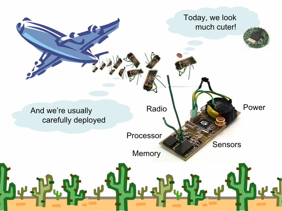
Power
Processor
Radio
SensorsMemory
Today, we look much cuter!
And we’re usually carefully deployed

Roger Wattenhofer, ETH Zurich @ Sirocco 2006 3
Distributed (Network) Algorithms
Roger Wattenhofer, ETH Zurich @ Sirocco 2006 4
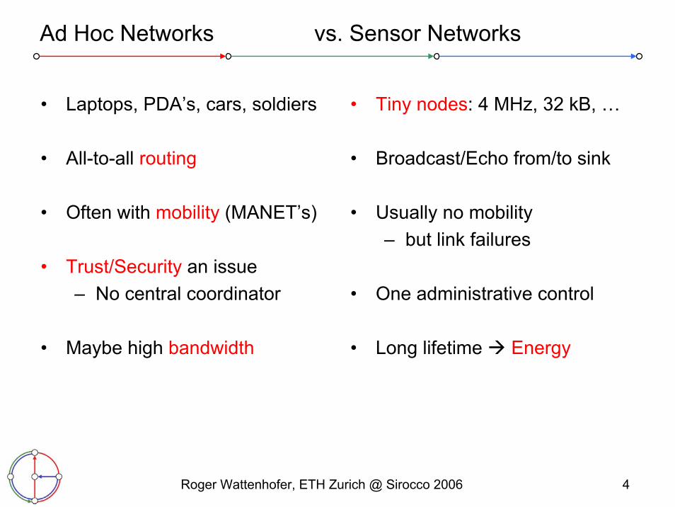
Ad Hoc Networks vs. Sensor Networks
• Laptops, PDA’s, cars, soldiers
• All-to-all routing
• Often with mobility (MANET’s)
• Trust/Security an issue– No central coordinator
• Maybe high bandwidth
• Tiny nodes: 4 MHz, 32 kB, …
• Broadcast/Echo from/to sink
• Usually no mobility– but link failures
• One administrative control
• Long lifetime Energy
Roger Wattenhofer, ETH Zurich @ Sirocco 2006 5
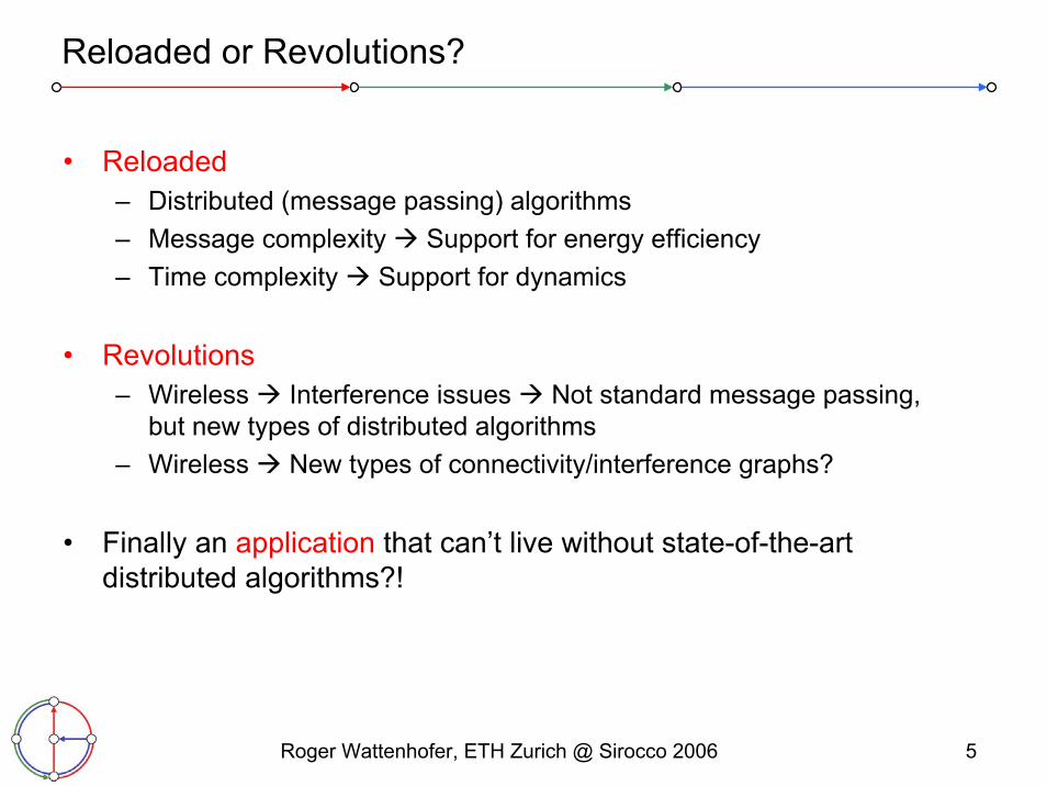
Reloaded or Revolutions?
• Reloaded– Distributed (message passing) algorithms– Message complexity Support for energy efficiency– Time complexity Support for dynamics
• Revolutions– Wireless Interference issues Not standard message passing,
but new types of distributed algorithms– Wireless New types of connectivity/interference graphs?
• Finally an application that can’t live without state-of-the-art distributed algorithms?!

Roger Wattenhofer, ETH Zurich @ Sirocco 2006 6
Overview
• Introduction
• Algorithmic Models: Case Study Clustering– Flooding vs. Dominating Sets– Non-Trivial Algorithm– Lower Bounds– Model Discussion
• Communication Models: Case Study Scheduling• Conclusions
Roger Wattenhofer, ETH Zurich @ Sirocco 2006 7
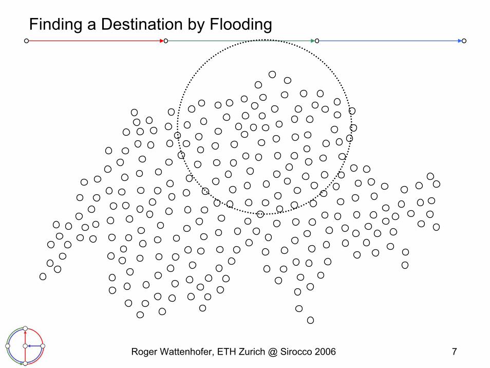
Finding a Destination by Flooding

Roger Wattenhofer, ETH Zurich @ Sirocco 2006 8
Finding a Destination Efficiently

Roger Wattenhofer, ETH Zurich @ Sirocco 2006 9
(Connected) Dominating Set
• A Dominating Set DS is a subset of nodes such that each node is either in DS or has a neighbor in DS.
• A Connected Dominating Set CDS is a connected DS, that is, there is a path between any two nodes in CDS that does not use nodes that are not in CDS.
• It might be favorable tohave few nodes in the (C)DS. This is known as theMinimum (C)DS problem.
Roger Wattenhofer, ETH Zurich @ Sirocco 2006 10
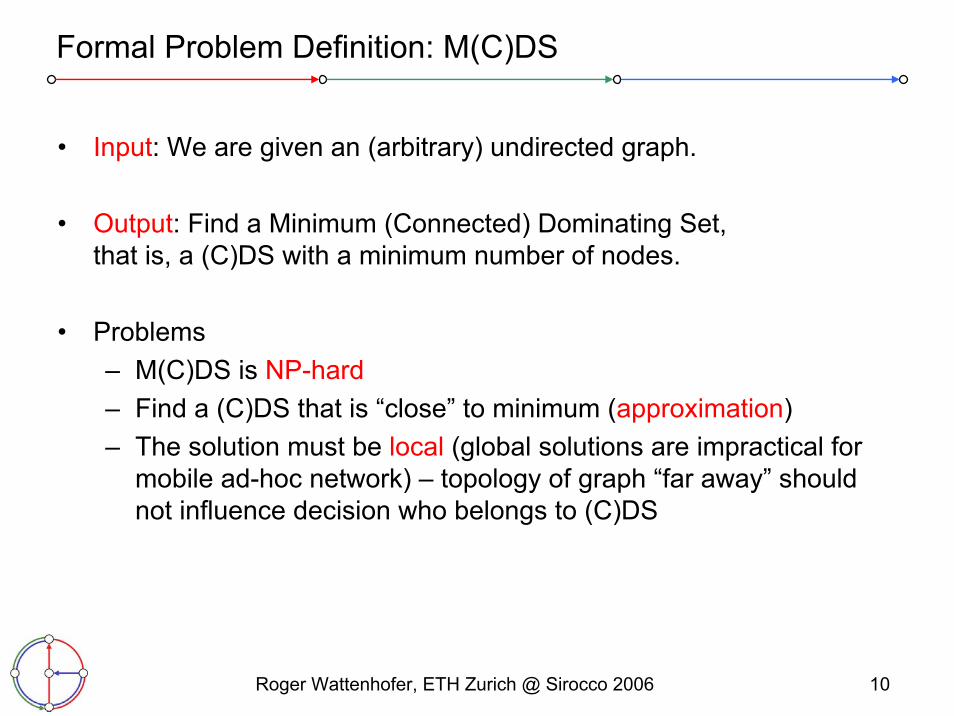
Formal Problem Definition: M(C)DS
• Input: We are given an (arbitrary) undirected graph.
• Output: Find a Minimum (Connected) Dominating Set,that is, a (C)DS with a minimum number of nodes.
• Problems– M(C)DS is NP-hard– Find a (C)DS that is “close” to minimum (approximation)– The solution must be local (global solutions are impractical for
mobile ad-hoc network) – topology of graph “far away” should not influence decision who belongs to (C)DS

Roger Wattenhofer, ETH Zurich @ Sirocco 2006 11
A Simple “Localized” Algorithm
• Classic greedy algorithm:
• “Always choose node with most non-dominated neighbors.”• The solution is a log-approximation (which is asymptotically
optimal, unless P ≈ NP).
• Distributed version:
1. Wait until higher-degree (same degree: higher-ID) neighbors have decided not to join dominating set.
2. Join dominating set and tell neighbors.
• Problem: This algorithm can have a linear waiting chain. Too slow!

Roger Wattenhofer, ETH Zurich @ Sirocco 2006 12
A Simple “Local” Algorithm
• If higher priority neighbors are connected and cover all other neighbors, then don’t join CDS, else join CDS– This talk, inspired by an improvement of Jie Wu– 2 rounds of communication for CDS only; lots of practical appeal– In the worst case very bad, even for UDGs only a √n approximation– However, on random UDGs, this gives a O(1) approximation
5
6
1
9
4
7
2
3
8

Roger Wattenhofer, ETH Zurich @ Sirocco 2006 13
Overview
• Introduction
• Algorithmic Models: Case Study Clustering– Flooding vs. Dominating Sets– Non-Trivial Algorithm– Lower Bounds– Model Discussion
• Communication Models: Case Study Scheduling• Conclusions
Roger Wattenhofer, ETH Zurich @ Sirocco 2006 14
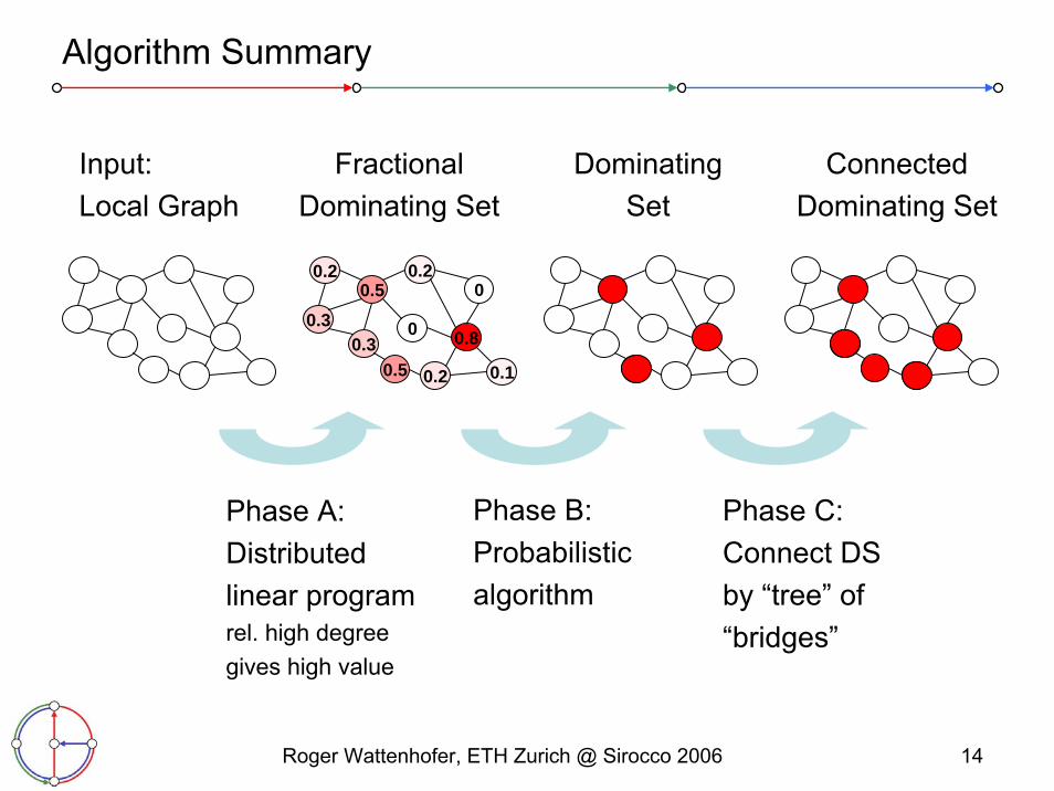
Algorithm Summary
0.20.5
0.2
0.80
0.2
0.3
0.10.3
0
Input:Local Graph
FractionalDominating Set
Dominating Set
ConnectedDominating Set
0.5
Phase C:Connect DS by “tree” of “bridges”
Phase B:Probabilisticalgorithm
Phase A:Distributedlinear programrel. high degree gives high value
Roger Wattenhofer, ETH Zurich @ Sirocco 2006 15
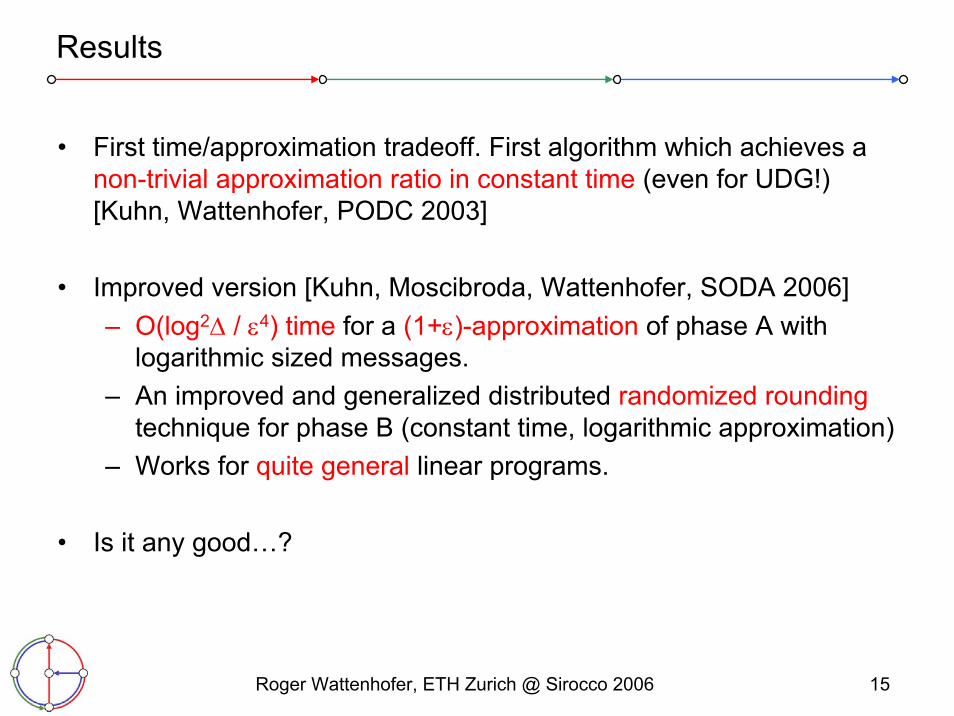
Results
• First time/approximation tradeoff. First algorithm which achieves a non-trivial approximation ratio in constant time (even for UDG!) [Kuhn, Wattenhofer, PODC 2003]
• Improved version [Kuhn, Moscibroda, Wattenhofer, SODA 2006]– O(log2Δ / ε4) time for a (1+ε)-approximation of phase A with
logarithmic sized messages.– An improved and generalized distributed randomized rounding
technique for phase B (constant time, logarithmic approximation)– Works for quite general linear programs.
• Is it any good…?
Roger Wattenhofer, ETH Zurich @ Sirocco 2006 16
Overview
• Introduction
• Algorithmic Models: Case Study Clustering– Flooding vs. Dominating Sets– Non-Trivial Algorithm– Lower Bounds– Model Discussion
• Communication Models: Case Study Scheduling• Conclusions
Roger Wattenhofer, ETH Zurich @ Sirocco 2006 17
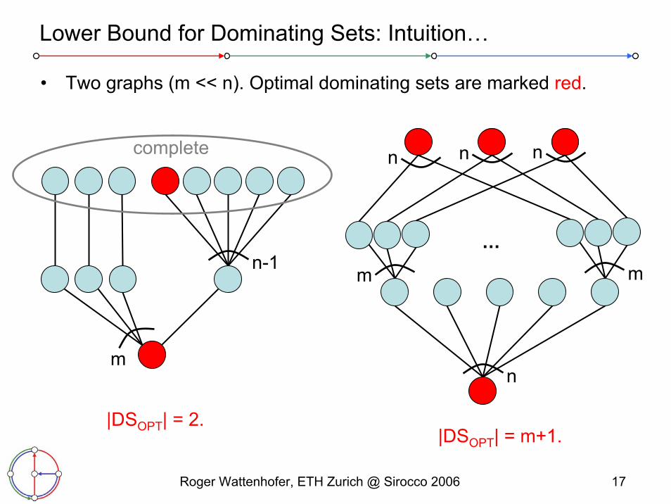
Lower Bound for Dominating Sets: Intuition…
m
n-1
complete
n
m m
…
n n n
• Two graphs (m << n). Optimal dominating sets are marked red.
|DSOPT| = 2.|DSOPT| = m+1.

Roger Wattenhofer, ETH Zurich @ Sirocco 2006 18
Lower Bound for Dominating Sets: Intuition…
• In local algorithms, nodes must decide only using local knowledge.• In the example green nodes see exactly the same neighborhood.
• So these green nodes must decide the same way!
m
n-1
n
m
…

Roger Wattenhofer, ETH Zurich @ Sirocco 2006 19
Lower Bound for Dominating Sets: Intuition…
m
n-1
complete
n
m m
…
n n n
• But however they decide, one way will be devastating (with n = m2)!
|DSOPT| = 2.|DSOPT without green| ≥ m.
|DSOPT| = m+1.|DSOPT with green| > n
Roger Wattenhofer, ETH Zurich @ Sirocco 2006 20
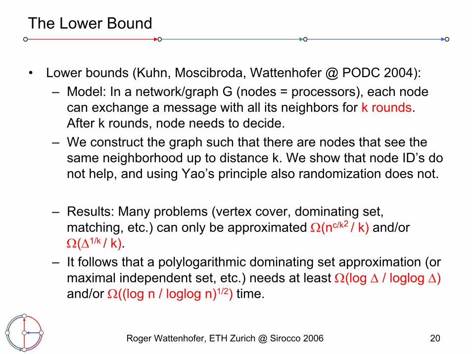
The Lower Bound
• Lower bounds (Kuhn, Moscibroda, Wattenhofer @ PODC 2004):– Model: In a network/graph G (nodes = processors), each node
can exchange a message with all its neighbors for k rounds. After k rounds, node needs to decide.
– We construct the graph such that there are nodes that see the same neighborhood up to distance k. We show that node ID’s do not help, and using Yao’s principle also randomization does not.
– Results: Many problems (vertex cover, dominating set, matching, etc.) can only be approximated Ω(nc/k2 / k) and/or Ω(Δ1/k / k).
– It follows that a polylogarithmic dominating set approximation (or maximal independent set, etc.) needs at least Ω(log Δ / loglog Δ)and/or Ω((log n / loglog n)1/2) time.

Roger Wattenhofer, ETH Zurich @ Sirocco 2006 21
Graph Used in Dominating Set Lower Bound
δ2 δ1δ3 δ0
δ0δ2δ3δ3 δ1 δ0δ0δ1δ2
δ2 δ0δ3 δ1 δ0 δ3 δ0δ2δ3δ2 δ1 δ0
δ2 δ1 δ0 δ3 δ2 δ0
• The example is for k = 3.• All edges are in fact special bipartite graphs
with large enough girth.

Roger Wattenhofer, ETH Zurich @ Sirocco 2006 22
Overview
• Introduction
• Algorithmic Models: Case Study Clustering– Flooding vs. Dominating Sets– Non-Trivial Algorithm– Lower Bounds– Model Discussion
• Communication Models: Case Study Scheduling• Conclusions

Roger Wattenhofer, ETH Zurich @ Sirocco 2006 23
Are Localized/Local Algorithms Practical?!?
• Localized algorithm: Causality chain, butterfly effect
• Local algorithm: Synchronous communication rounds– Quite high demand to MAC layer– In reality messages get lost, due to fading, noise, and interference– In reality not all neighbors receive a message (hidden terminal problem)– In reality nodes might crash and restart (shabby power supply)
• Smells like self-stabilization– Messages might get lost, duplicated, or corrupted– Node memory/state might get corrupted (RAM only)– However, ROM (program, initialization, random seed) is safe
Roger Wattenhofer, ETH Zurich @ Sirocco 2006 24
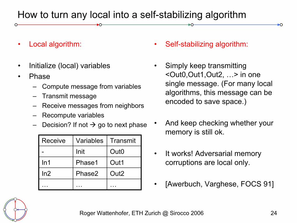
How to turn any local into a self-stabilizing algorithm
• Local algorithm:
• Initialize (local) variables• Phase
– Compute message from variables– Transmit message– Receive messages from neighbors– Recompute variables– Decision? If not go to next phase
• Self-stabilizing algorithm:
• Simply keep transmitting <Out0,Out1,Out2, …> in one single message. (For many local algorithms, this message can be encoded to save space.)
• And keep checking whether your memory is still ok.
• It works! Adversarial memory corruptions are local only.
• [Awerbuch, Varghese, FOCS 91]
Receive Variables Transmit- Init Out0In1 Phase1 Out1In2 Phase2 Out2… … …

Roger Wattenhofer, ETH Zurich @ Sirocco 2006 25
Algorithm Classes
Global Algorithm
Distributed Algorithm
Local Localized
• For some problems we don’t evenunderstand the non-distributed case
• “Reiceive msg X Transmit msg Y”• Every global algo can be distributed
+ Node can only communicate with neighbors k times.
+ Strict time bounds– Synchronous model
Unstructured
+ Often simple– Nodes can wait for
neighbor actions– Often linear chain
of causality
+ Implement MAC layer yourself; you control everything
– Often complicated– Argumentation
overhead

Roger Wattenhofer, ETH Zurich @ Sirocco 2006 26
Clustering for Unstructured Radio Networks
• “Big Bang” (deployment) of a sensor and/or ad-hoc network:– Nodes wake up asynchronously (very late, maybe)– Neighbors unknown– Hidden terminal problem– No global clock– No established MAC protocol– No reliable collision detection – Limited knowledge of the number of nodes or degree of network.
• We have randomized algorithms that compute DS (or MIS) in polylog(n) time even under these harsh circumstances, where n is an upper bound on the number of nodes in the system.
• [Kuhn, Moscibroda, Wattenhofer @ MobiCom 2004]
Roger Wattenhofer, ETH Zurich @ Sirocco 2006 27
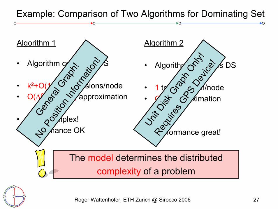
The model determines the distributedcomplexity of a problem
Example: Comparison of Two Algorithms for Dominating Set
Algorithm 1
• Algorithm computes DS
• k2+O(1) transmissions/node• O(ΔO(1)/k log Δ) approximation
• Quite complex!• Performance OK
Algorithm 2
• Algorithm computes DS
• 1 transmission/node• O(1) approximation
• Easy!• Performance great!
Gener
al Gra
ph!
No Pos
ition I
nform
ation
!
Unit D
isk G
raph
Only
!
Requir
es G
PS D
evice
!

Roger Wattenhofer, ETH Zurich @ Sirocco 2006 28
Connectivity Models
too pessimistic too optimistic
GeneralGraph
UDG
QuasiUDG
d
1
Bounded Independence
Unit BallGraph
Roger Wattenhofer, ETH Zurich @ Sirocco 2006 29
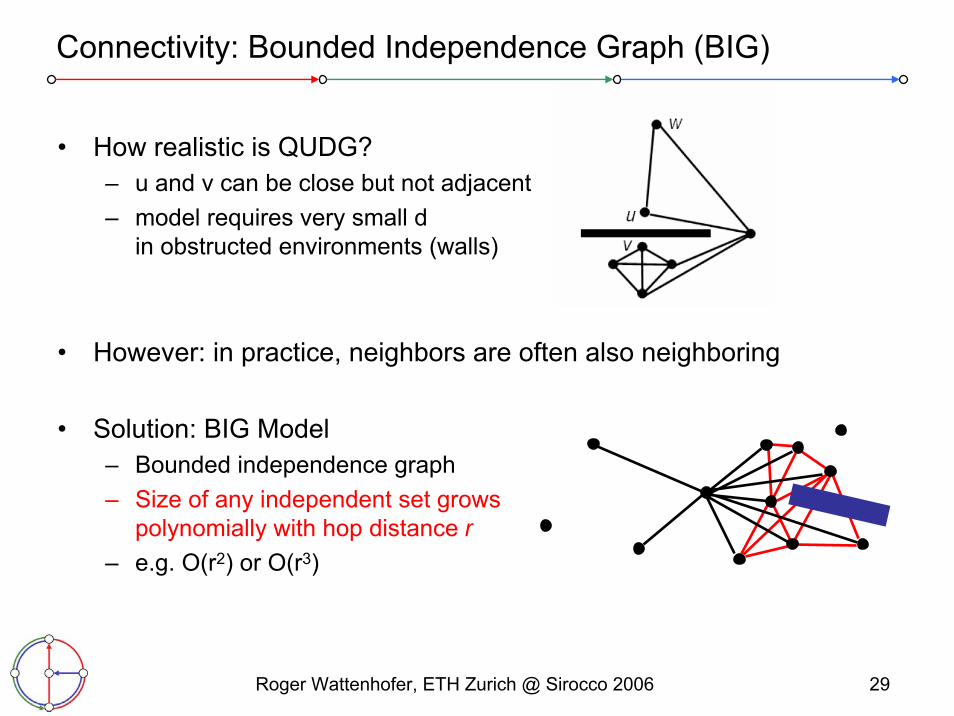
Connectivity: Bounded Independence Graph (BIG)
• How realistic is QUDG?– u and v can be close but not adjacent– model requires very small d
in obstructed environments (walls)
• However: in practice, neighbors are often also neighboring
• Solution: BIG Model– Bounded independence graph– Size of any independent set grows
polynomially with hop distance r– e.g. O(r2) or O(r3)

Roger Wattenhofer, ETH Zurich @ Sirocco 2006 30
Connectivity: Unit Ball Graph (UBG)
• ∃ metric (V,d) describing distances between nodes u,v ∈ V
such that: d(u,v) · 1 : (u,v) ∈ Esuch that: d(u,v) > 1 : (u,v) ∈ E
• Assume that doubling dimension of metric is constant– Doubling dimension: log(#balls of radius r/2 to cover ball of radius r)
UBG based onunderlying doubling metric.

Roger Wattenhofer, ETH Zurich @ Sirocco 2006 31
Models can be put in relation
• Try to proof correctness in an as “high” as possible model• For efficiency, a more optimistic (“lower”) model might be fine
[Schmid, Wattenhofer, WPDRTS 2006]
Roger Wattenhofer, ETH Zurich @ Sirocco 2006 32
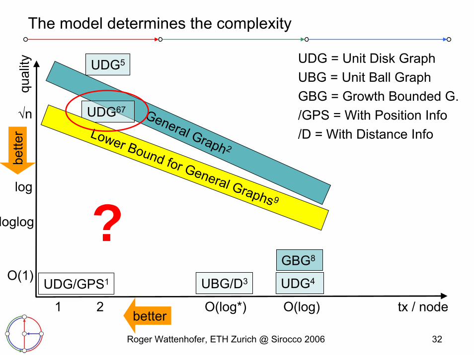
The model determines the complexity
tx / node
qual
ity
O(1)
log
√n
1 2 O(log*) O(log)
General Graph 2
UDG67
UDG4
UDG5
UDG/GPS1
GBG8
UDG = Unit Disk GraphUBG = Unit Ball GraphGBG = Growth Bounded G./GPS = With Position Info/D = With Distance InfoLower Bound for General Graphs9
bette
r
better
UBG/D3
loglog ?
Roger Wattenhofer, ETH Zurich @ Sirocco 2006 33
References
1. Folk theorem, e.g. Kuhn, Wattenhofer, Zhang, Zollinger, PODC 20032. Kuhn, Wattenhofer, PODC 2003
• Improved: Kuhn, Moscibroda, Wattenhofer, SODA 2006• CDS by Dubhashi et al, SODA 2003
3. Kuhn, Moscibroda, Wattenhofer, PODC 20054. Alzoubi, Wan, Frieder, MobiHoc 20025. Wu and Li, DIALM 19996. Gao, Guibas, Hershberger, Zhang, Zhu, SCG 20017. Wattenhofer, MedHocNet 2005 talk, Improving on Wu and Li8. Kuhn, Moscibroda, Nieberg, Wattenhofer, DISC 2005 9. Kuhn, Moscibroda, Wattenhofer, PODC 2004
Roger Wattenhofer, ETH Zurich @ Sirocco 2006 34
Overview
• Introduction• Algorithmic Models: Case Study Clustering
• Communication Models: Case Study Scheduling– Introduction– Intuition & Results– Lower Bound Example– From Theory to Practice
• Conclusions
Roger Wattenhofer, ETH Zurich @ Sirocco 2006 35
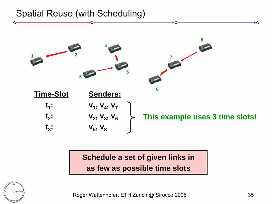
1
Spatial Reuse (with Scheduling)
2
3
4
5
8
7
6Time-Slot Senders:
t1: v1, v4, v7
t2: v2, v3, v6
t3: v5, v8
This example uses 3 time slots!
Schedule a set of given links in as few as possible time slots

Roger Wattenhofer, ETH Zurich @ Sirocco 2006 36
Physical Model
• Let us look at the signal-to-noise-plus-interference (SINR) ratio!• Message arrives if SINR is larger than β at receiver
Minimum signal-to-interference ratio
Power level of sender u
Path-loss exponent
Noise
Distance betweentwo nodes
Roger Wattenhofer, ETH Zurich @ Sirocco 2006 37
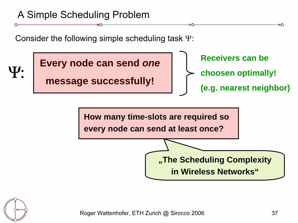
Consider the following simple scheduling task Ψ:
A Simple Scheduling Problem
Every node can send one
message successfully!
Receivers can be
choosen optimally!
(e.g. nearest neighbor)
How many time-slots are required soevery node can send at least once?
„The Scheduling Complexityin Wireless Networks“
Ψ:
Roger Wattenhofer, ETH Zurich @ Sirocco 2006 38
Overview
• Introduction• Algorithmic Models: Case Study Clustering
• Communication Models: Case Study Scheduling– Introduction– Intuition & Results– Lower Bound Example– From Theory to Practice
• Conclusions

Roger Wattenhofer, ETH Zurich @ Sirocco 2006 39
• Let α=3, β=3, and N=10nW (realistic values!)• Set the transmission powers as follows PC= -7 dBm and PA= 0 dBm
• SINR at D is:
• SINR at B is:
Can we schedule links concurrently…?
A B C D
1m 1m 1m
A wants to sent to B, C wants to send to D
Simultaneous transmission is possible !

Roger Wattenhofer, ETH Zurich @ Sirocco 2006 40
Let’s make it tougher!
A BC D1m
A wants to sent to B, C wants to send to D
• Let α=3, β=3, and N=10nW• Set the transmission powers as follows PC= -15 dBm and PA= 1 dBm
• SINR at D is:
• SINR at B is:
Simultaneous transmission is possible !
4m 2m
Roger Wattenhofer, ETH Zurich @ Sirocco 2006 41
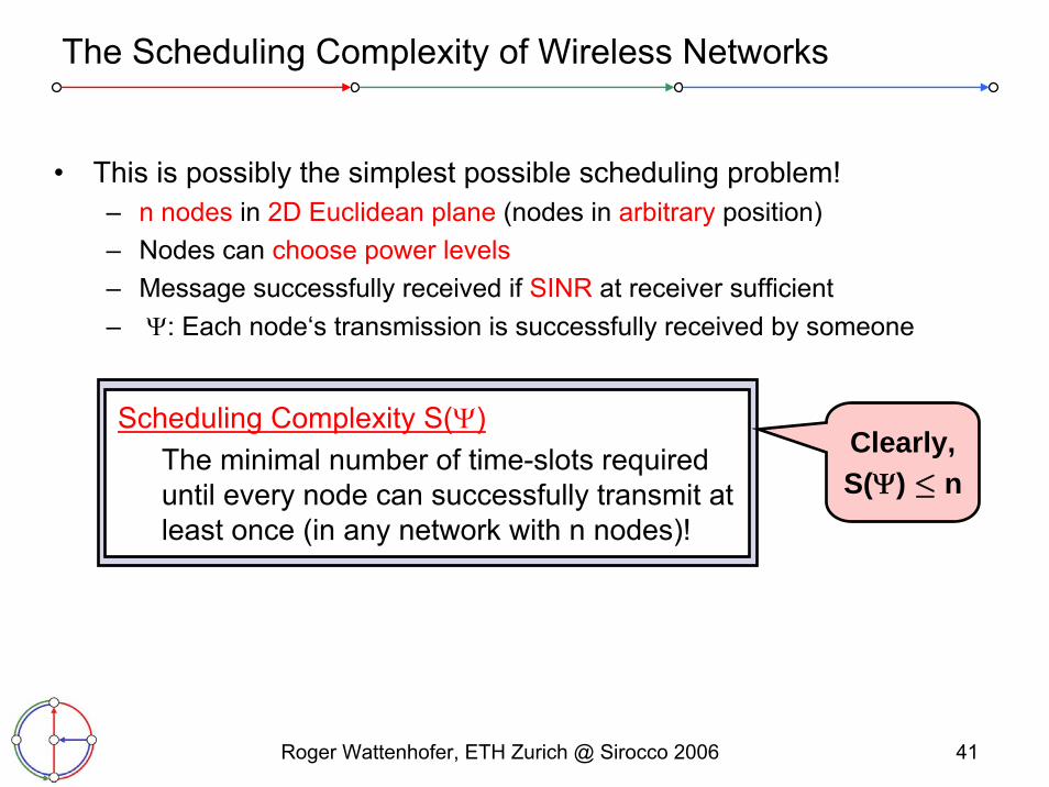
• This is possibly the simplest possible scheduling problem!– n nodes in 2D Euclidean plane (nodes in arbitrary position)– Nodes can choose power levels– Message successfully received if SINR at receiver sufficient– Ψ: Each node‘s transmission is successfully received by someone
The Scheduling Complexity of Wireless Networks
Clearly,S(Ψ) · n
Scheduling Complexity S(Ψ)The minimal number of time-slots requireduntil every node can successfully transmit at least once (in any network with n nodes)!
Roger Wattenhofer, ETH Zurich @ Sirocco 2006 42
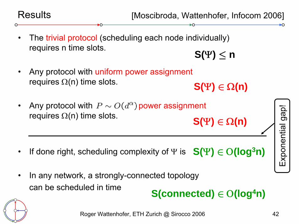
• The trivial protocol (scheduling each node individually) requires n time slots.
• Any protocol with uniform power assignmentrequires Ω(n) time slots.
• Any protocol with power assignmentrequires Ω(n) time slots.
• If done right, scheduling complexity of Ψ is
• In any network, a strongly-connected topologycan be scheduled in time
S(Ψ) · n
S(Ψ) ∈ Ω(n)
S(Ψ) ∈ Ω(n)
Results [Moscibroda, Wattenhofer, Infocom 2006]
S(Ψ) ∈ Ο(log3n)
S(connected) ∈ Ο(log4n)
Exp
onen
tial g
ap!

Roger Wattenhofer, ETH Zurich @ Sirocco 2006 43
Overview
• Introduction• Algorithmic Models: Case Study Clustering
• Communication Models: Case Study Scheduling– Introduction– Intuition & Results– Lower Bound Example– From Theory to Practice
• Conclusions

Roger Wattenhofer, ETH Zurich @ Sirocco 2006 44
Lower Bound for Power Assignment
• Consider the exponential chain:

Roger Wattenhofer, ETH Zurich @ Sirocco 2006 45
• Consider the exponential chain:
• Exponential chain can be scheduled in O(1) time!• How many links can we schedule simultaneously with ?• Consider first node v1...
its power is P1=ρ210α for some constant ρ• This creates interference of at least ρ/2α at every other node! • The second node v2 also sends with power P2=ρ27α
• Again, this creates an additional interference of at least ρ/2α at everyother node!
1
v1v2
2 22 23 24 25 26 27 28 29 210
f1
ρ(f1)α Power
Interference>ρ/2α>ρ/2α>ρ/2α>ρ/2α>ρ/2α>ρ/2α>ρ/2αρ(f2)α
f2
>ρ/2α>ρ/2α >ρ/2α
Lower Bound for Power Assignment
Not trivial…
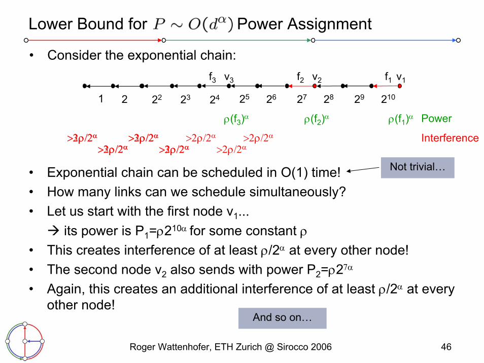
Roger Wattenhofer, ETH Zurich @ Sirocco 2006 46
• Consider the exponential chain:
• Exponential chain can be scheduled in O(1) time!• How many links can we schedule simultaneously?• Let us start with the first node v1...
its power is P1=ρ210α for some constant ρ• This creates interference of at least ρ/2α at every other node! • The second node v2 also sends with power P2=ρ27α
• Again, this creates an additional interference of at least ρ/2α at everyother node!
1
v1
Power
Interference>2ρ/2α
>2ρ/2αρ(f2)α
v2
>2ρ/2α >2ρ/2α>2ρ/2α>2ρ/2α
>2ρ/2α
2 22 23 24 25 26 27 28 29 210
f1
ρ(f1)α
f2
And so on…
v3
ρ(f3)α
>3ρ/2α>3ρ/2α
>3ρ/2α>3ρ/2α
f3
Lower Bound for Power Assignment
Not trivial…
Roger Wattenhofer, ETH Zurich @ Sirocco 2006 47
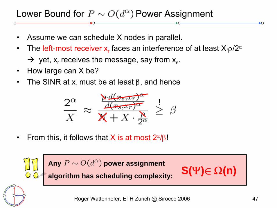
• Assume we can schedule X nodes in parallel. • The left-most receiver xr faces an interference of at least X·ρ/2α
yet, xr receives the message, say from xs. • How large can X be?• The SINR at xr must be at least β, and hence
• From this, it follows that X is at most 2α/β!
Lower Bound for Power Assignment
Any power assignment
algorithm has scheduling complexity: S(Ψ)∈ Ω(n)
!

Roger Wattenhofer, ETH Zurich @ Sirocco 2006 48
Overview
• Introduction• Algorithmic Models: Case Study Clustering
• Communication Models: Case Study Scheduling– Introduction– Intuition & Results– Lower Bound Example– From Theory to Practice
• Conclusions

Roger Wattenhofer, ETH Zurich @ Sirocco 2006 49
Observations and Implications
• All MAC layer protocols we are aware of use either uniform or dα
power assignment. – Thus, the theoretical performance of current MAC layer protocols
almost as bad as scheduling every single node individually!
• In contrast: faster polylogarithmic scheduling (faster MAC protocols) are theoretically possible in all (even worst-case) networks, if nodes choose power carefully.– Theoretically, there is no fundamental scaling problem with scheduling
(in contrast to capacity). – Theoretically efficient MAC protocols must use non-trivial power levels!
• Well, the word theory appeared in every line...

Roger Wattenhofer, ETH Zurich @ Sirocco 2006 50
From Theory to Practice
• We did measurements using standard mica2 nodes!
• Replaced standard MAC protocol by a (tailor-made) „SINR-MAC“
• Measured for instance the following deployment...
• Time for successfully transmitting 20‘000 packets:
Speed-up is almost a factor 3
u1 u2 u3 u4 u5 u6

Roger Wattenhofer, ETH Zurich @ Sirocco 2006 51
Possible Applications – Improved “Channel Capacity”
• Consider a channel consisting of wireless sensor nodes
• What throughput-capacity of this channel...?
time Channel capacity is 1/3
Roger Wattenhofer, ETH Zurich @ Sirocco 2006 52
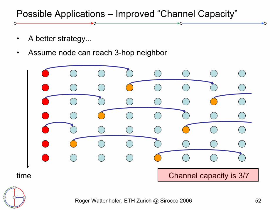
Possible Applications – Improved “Channel Capacity”
• A better strategy...
• Assume node can reach 3-hop neighbor
time Channel capacity is 3/7

Roger Wattenhofer, ETH Zurich @ Sirocco 2006 53
Possible Applications – Improved “Channel Capacity”
• All such (graph-based) strategies have capacity strictly less than 1/2!
• For certain α and β, the following strategy is better!
time Channel capacity is 1/2
Roger Wattenhofer, ETH Zurich @ Sirocco 2006 54
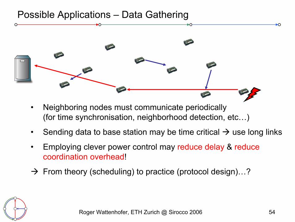
• Neighboring nodes must communicate periodically (for time synchronisation, neighborhood detection, etc…)
• Sending data to base station may be time critical use long links
• Employing clever power control may reduce delay & reduce coordination overhead!
From theory (scheduling) to practice (protocol design)…?
Possible Applications – Data Gathering

Roger Wattenhofer, ETH Zurich @ Sirocco 2006 55
Overview
• Introduction• Algorithmic Models: Case Study Clustering• Communication Models: Case Study Scheduling
• Conclusions

Roger Wattenhofer, ETH Zurich @ Sirocco 2006 56
More…
Link Layer
Network Layer
Services
Theory/Models
• Clustering (Dominating Sets, etc.)• Interference and Signal-to-Noise-Ratio • MAC Layer and Coloring• Topology and Power Control • Deployment (Unstructured Radio Networks) • New Routing Paradigms (e.g. Link Reversal)• Geo-Routing • Broadcast and Multicast • Data Gathering • Location Services and Positioning • Time Synchronization• Modeling and Mobility • Lower Bounds for Message Passing• Selfish Agents, Economic Aspects, Security

Roger Wattenhofer, ETH Zurich @ Sirocco 2006 57
Summary
• Sensor networks are an excellent application for distributed algorithms
• We need to study new network topologies– Network models between geometry and graph theory (BIG, UBG)– Interference models such as SINR
• We need to study new algorithmic paradigms– Distributed Localized Local Self-Stabilizing Unstructured
Roger Wattenhofer, ETH Zurich @ Sirocco 2006 58
Thank You!Questions? Comments?