sensorless control of a hybrid stepper motor - diva portal939441/fulltext01.pdf · sensorless...
TRANSCRIPT
Master of Science Thesis in Electrical EngineeringDepartment of Electrical Engineering, Linköping University, 2016
Sensorless Control of aHybrid Stepper Motor
Lina Karlsson
Master of Science Thesis in Electrical Engineering
Sensorless Control of a Hybrid Stepper Motor
Lina Karlsson
LiTH-ISY-EX--16/4962--SE
Supervisor: Sergii Voronovisy, Linköping University
Stefan GrufmanHusqvarna AB
Examiner: Mattias Krysanderisy, Linköping University
Division of Automatic ControlDepartment of Electrical Engineering
Linköping UniversitySE-581 83 Linköping, Sweden
Copyright © 2016 Lina Karlsson
Abstract
Electrical drives are widely used in today’s society. They can be found in bothhousehold products and in the industry. One application where electrical drivesare used is in robots for mowing lawns. In the studied robots the motors in theelectrical drives used for propulsion are Brush Less Direct Current motors, BLDC-motors. The BLDC-motor has its maximum torque at high speeds and thereforea gearbox is needed. The gearbox is space consuming, add costs and consists ofmechanical parts that wear during use. Of interest is therefore to investigate ifthere are other electrical drives which can be used for propulsion.
A motor who has its maximum torque at low speeds is the Stepper motor, andtherefore it is of interest to investigate if a stepper motor could replace the BLDC-motor. A drawback with the stepper motor is that it always consumes maximumcurrent and therefore a current controller is beneficial. Together with currentcontrol, speed control is needed to make the robot run at desired speed. To beable to perform an accurate current and speed control feedback from the motor isneeded. Information about the rotor angle and velocity can be used for the speedcontrol and the load angle can be used for the current control since the current isproportional to the load torque.
To estimate the rotor angle and velocity a model has been developed. Themodel is based on fundamental electrical and mechanical equations and neglectsthe current and position dependence of the inductance and flux linkage. To com-plete the model three motor parameters, the maximum detent torque Tdm, themaximum flux linkage ψm and the friction constant Bwas determined. Parameterdetermination was done by linear regression and by using an Extended KalmanFilter, EKF. The result of the parameter determination were Tdm = 0.2152 Nm,ψm = -0.002854 Vs/rad and B = 0.01186 Nms/rad.
The model is used in an EKF to estimate the rotor angle and angular velocity.The result of the implemented EKF seems promising. When making the rotortake a step in velocity from 3.927 rad/s to 7.85 rad/s the EKF estimates the stateswith only a small bias: 0.02 rad for the angle, 0.3 rad/s for the velocity, 0.005 Afor phase a current and 0.0004 A for phase b current.
To estimate the load angle the Sliding Discrete Fourier Transform is used. Theexpected relation between the load torque and load angle is sinusoidal. The loadangle is calculated from data where the external load is between 0-2.5 Nm. Inthat area the load angle shows the expected sinusoidal appearance and the loadangle is in the area between 0.1 and 0.45 rad. At 3 Nm the rotor stalls and it isshown that the load angle varies between 0 and 2π rad when the rotor is stalled.
iii


Acknowledgments
First of all, I want to begin by thanking Husqvarna AB for providing me with theopportunity to perform this master’s thesis work. I want to show my gratitudeto all who have supported me. Especially thanks to Magnus Öhrlund for intro-ducing me to the project and describing potentials of stepper motors, Pär-OlaSvensson for your support with the equipment, Martin Larsén for sharing yourknowledge about motors, Jonas Rangsjö for your help with the EKF, and finallyStefan Grufman for organizing everything.
I also want to express my gratitude to my examiner Mattias Krysander andsupervisor Sergii Voronov. They have always been available for discussions re-garding the motor model, estimation methods and implementation problems.
Finally, I want to thank my family for helping me through seventeen years ofstudies, and my fiancé, Mattias Lindbäck, for encouraging me and always believ-ing in me.
Linköping, June 2016Lina Karlsson
v

Contents
Notation ix
1 Introduction 11.1 Motivation . . . . . . . . . . . . . . . . . . . . . . . . . . . . . . . . 21.2 Problem formulation . . . . . . . . . . . . . . . . . . . . . . . . . . 21.3 Outline . . . . . . . . . . . . . . . . . . . . . . . . . . . . . . . . . . 3
2 Related work 5
3 Theoretical background 73.1 Hybrid Stepper Motor . . . . . . . . . . . . . . . . . . . . . . . . . . 73.2 Load Angle . . . . . . . . . . . . . . . . . . . . . . . . . . . . . . . . 93.3 Sliding Discrete Fourier Transform . . . . . . . . . . . . . . . . . . 113.4 Multiple linear regression . . . . . . . . . . . . . . . . . . . . . . . 123.5 Residual analysis . . . . . . . . . . . . . . . . . . . . . . . . . . . . 123.6 Extended Kalman Filter . . . . . . . . . . . . . . . . . . . . . . . . . 13
4 Data collection 154.1 Equipment setup . . . . . . . . . . . . . . . . . . . . . . . . . . . . 154.2 Collected Data . . . . . . . . . . . . . . . . . . . . . . . . . . . . . . 17
5 Modeling 235.1 Motor model . . . . . . . . . . . . . . . . . . . . . . . . . . . . . . . 23
6 Determination of unknown motor parameters 276.1 Determination of parameters individually . . . . . . . . . . . . . . 27
6.1.1 Detent torque . . . . . . . . . . . . . . . . . . . . . . . . . . 276.1.2 Friction constant . . . . . . . . . . . . . . . . . . . . . . . . 276.1.3 Maximum flux linkage . . . . . . . . . . . . . . . . . . . . . 30
6.2 Determination with multiple linear regression . . . . . . . . . . . . 326.3 Determination with the Extended Kalman Filter . . . . . . . . . . 34
6.3.1 Choose filter parameters . . . . . . . . . . . . . . . . . . . . 376.4 Residual analysis . . . . . . . . . . . . . . . . . . . . . . . . . . . . 39
vii
viii Contents
7 Estimations 457.1 Extended Kalman Filter . . . . . . . . . . . . . . . . . . . . . . . . . 457.2 Load angle estimation . . . . . . . . . . . . . . . . . . . . . . . . . . 46
8 Results 498.1 Evaluation of model and model parameters . . . . . . . . . . . . . 498.2 Evaluation of the EKF . . . . . . . . . . . . . . . . . . . . . . . . . . 508.3 Evaluation of load angle estimations . . . . . . . . . . . . . . . . . 51
9 Discussion 599.1 Results . . . . . . . . . . . . . . . . . . . . . . . . . . . . . . . . . . 59
9.1.1 Motor model and parameters . . . . . . . . . . . . . . . . . 599.1.2 EKF and load angle . . . . . . . . . . . . . . . . . . . . . . . 60
9.2 Future work . . . . . . . . . . . . . . . . . . . . . . . . . . . . . . . 619.2.1 Parameter determination . . . . . . . . . . . . . . . . . . . . 619.2.2 Extended Kalman Filter . . . . . . . . . . . . . . . . . . . . 629.2.3 Load angle . . . . . . . . . . . . . . . . . . . . . . . . . . . . 62
10 Conclusions 63
Bibliography 65
Notation
Acronyms
Acronym Meaning
ACF Autocorrelation FunctionBLDC Brush Less Direct CurrentDFT Discrete Fourier TransformEKF Extended Kalman FilterEMF Electromotive ForceHSM Hybrid Stepper MotorODE Ordinary Differential EquationOLS Ordinary Least SquaresRSS Residual Sum of Squares
SDTF Sliding Discrete Fourier Transform
Symbols
Symbol Meaning
L inductance [H]R resistance [Ω]J inertia [kgm2]B friction coefficient [Nms/rad]ej back electromotive force for phase j [Vs]ψ flux linkage [Vs/rad]
ψmax maximum flux linkage [Vs/rad]θ rotor angle [rad]ω rotor angular velocity [rad/s]ij phase j current [A]vj phase j voltage [V]Tj torque produced by phase j [Nm]TD detent torque [Nm]TL load torque [Nm]δ load angle [rad]
ix

1Introduction
Everywhere in today’s society, it is possible to come across products whose func-tionality is based on motion. In most households you probably can find productssuch as household appliances, tools, watches, fans, hair dryers, printers and toys,and in the industry you can find robots, vehicles, elevators, escalators, rollingmills and pumps. What enables the movement in all these products are electricaldrives.
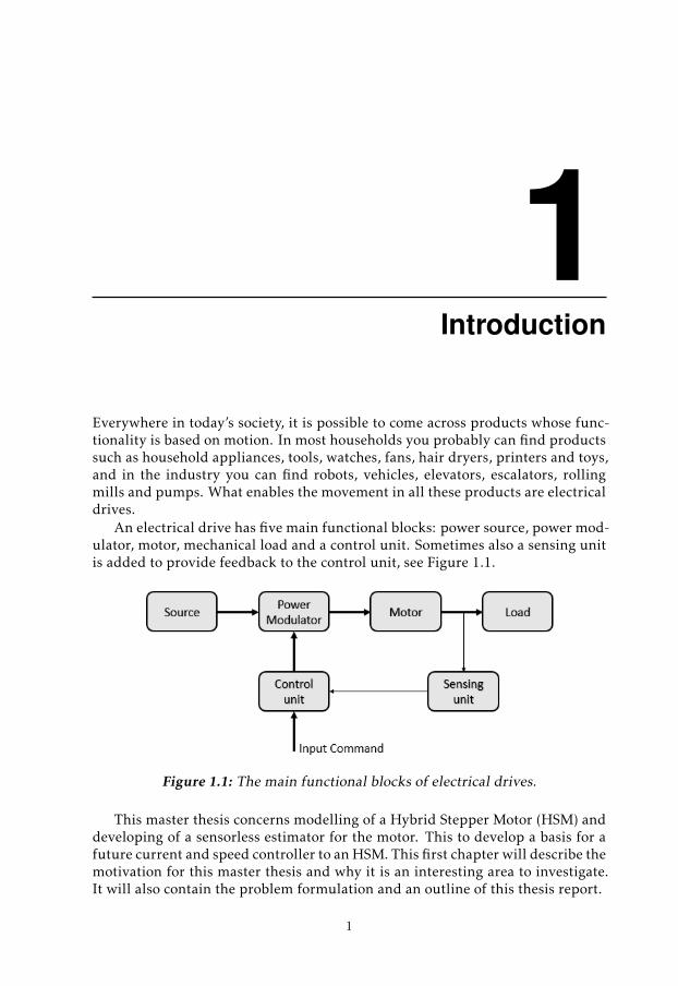
An electrical drive has five main functional blocks: power source, power mod-ulator, motor, mechanical load and a control unit. Sometimes also a sensing unitis added to provide feedback to the control unit, see Figure 1.1.
Figure 1.1: The main functional blocks of electrical drives.
This master thesis concerns modelling of a Hybrid Stepper Motor (HSM) anddeveloping of a sensorless estimator for the motor. This to develop a basis for afuture current and speed controller to an HSM. This first chapter will describe themotivation for this master thesis and why it is an interesting area to investigate.It will also contain the problem formulation and an outline of this thesis report.
1
2 1 Introduction
1.1 Motivation
Husqvarna AB has developed and sold autonomous robots for mowing lawnsfor 20 years. Important factors are that the robots are energy efficient, not tooexpensive to manufacture and long lasting without need to repair it.
Today, the motors used for robots propulsion are Brush Less Direct Currentmotors (BLDC-motor). The BLDC-motor has its maximum torque at a speedabove the speed the robot will be run in. Therefore, a gearbox is needed to obtainthe desired torque at lower speeds. The disadvantage with this solution is thatthe gearbox is space consuming, increases the cost of the robot and consists ofmechanical parts that wear during use. For that reason it is of interest to inves-tigate if there are other motors that can be used for propulsion without use of agearbox.
A motor with its maximum torque at low speeds is the stepper motor. The ad-vantage with this motor is thus that a gearbox is not necessary to obtain desiredtorque at low speeds. A stepper motor is also cheaper than a BLDC-motor. There-fore, introduction of a stepper motor instead of current technology can reducethe cost of the robot, decrease the space of the motor solution and eliminate theproblem with worn out gearboxes.
To be able to replace the motor, a new control algorithm needs to be devel-oped. If the load is fixed during drive, a stepper motor can be controlled by anopen loop method. However, open loop control often results in torque and speedripples, noise, vibrations, a poor energy efficiency and no control on step loss. Toavoid step loss, motor applications based on open loop control often are drivenwith maximum current which is not preferable for battery applications.
For applications where the load will vary during drive, a closed loop controlis preferred. For closed loop control the most straightforward method is to usea rotor position sensor. A mechanical sensor increase cost and size of the motorand Husqvarna therefore wants a sensorless solution.
1.2 Problem formulation
The purpose is to investigate if it is possible to develop a sensorless estimatorfor a hybrid stepper motor and discuss if the outcome from the estimator canbe used to perform a sensorless speed and torque control on a Hybrid StepperMotor (HSM). To be able to do an accurate speed and torque control of the motorfeedback such as rotor angle, rotor velocity and the load angle can be used. Thesensorless estimator will use the phase current and phase voltages of the motorto estimate above mentioned states. Due to the lack of hardware, the model andestimator will only be implemented and tested in a simulation environment.
If the result looks promising Husqvarna AB has a basis for further investiga-tion of stepper motors and its potential to replace the BLDC-motors. Furtherthis can decrease the cost of the robot and also increase the lifespan of the motorsolution.

1.3 Outline 3
1.3 Outline
The thesis is organized in several chapters. Chapter 2 shortly describes the re-lated work to this thesis and which kind of solutions that have been used forsimilar problems. Chapter 3 introduces the background theory of the thesis. InChapter 4 the equipment for data collection is described. Chapter 5 describesthe model of the HSM which will be used in further investigations of the HSM.The model contains of unknown parameters, and how to determine these aredescribed in Chapter 6. In Chapter 7 an Extended Kalman filter is introducedfor estimation of the rotor angle and rotor position. In the end of the chapter amethod of estimating the load angle is presented. Chapter 8 presents the resultsof the model and estimator in Matlab. Chapter 9 discusses the result and thefuture work in this area. Finally, a conclusion is made in Chapter 10.

2Related work
The modern stepping motor was first invented in 1957 by Thomas and Fleis-chauer [10]. Stepping motors are often used in digital control systems wherethe motor receives open loop commands, in shape of train pulses, to rotate toa specific angle [16]. This makes stepping motors suitable in printers, plotters,CD-players and for tool positioning [16]. But due to the rotor inertia, the rotoroscillates around the goal position before stabilizing which creates an jerky mo-tion of the rotor. Because of this the motor can loose steps if the variation ofthe load torque is too fast [2]. Usage of programmable architectures like field-programmable gate arrays circuits together with advanced control algorithms en-ables microstepping of the motors. This makes the rotor motion smoother butproblem with step loss still remains [2], [7]. The control algorithms can also op-timize the torque dynamics in the motor [7]. To work properly these algorithmsneeds feedback, such as rotor position or rotor flux, from the motor. This meansthat a closed loop control needs to be introduced. A closed loop control can beperformed either with a positioning sensor or with a rotor position estimator. Aposition sensor adds costs and complexity, and increase the size of the system.Therefore it is of interest to provide feedback from a positioning estimator in-stead [7].
A commonly proposed estimator is the Extended Kalman Filter, EKF, whichis used to estimate the rotor position and velocity [2], [4], [14]. To be able toimplement an EKF a state space model of the motor is needed. Authors in [2],[14] and [15] proposes a model based on fundamental electrical and mechanicalequations. The model represents the motor phases separately. According to au-thors in [2] this is because the Hybrid Stepper Motor has its two phases, a andb, in quadrature. The electrical equations neglects the position and current de-pendence of the permanent magnet flux linkage and inductance. According toauthors in [4] this could lead to poor model fit since the significance of the posi-
5
6 2 Related work
tion and current dependence may not always be negligible. However, adding thisdependence increases the complexity of the model and how much the model fitwill increase depends on the available hardware. A decision must also be madeif a more complex model is worth an increase in computational costs [4].
The models proposed in [2], [4], [14] and [15] are mostly used for speed andposition control and in situations where the load torque is small or varies slowly.In the suggested models the load torque is an unknown source of disturbance andto increase the overall robustness of the system it is useful to also use the EKF toestimate the load torque. To be able to estimate the load torque it is added as afifth state and an equation explaining the load torque variations is added in themodel [14].
To be able to get more information about the load another possibility is toestimate the load angle [5], [6], [7]. The load angle describes the lag between theinstantaneous rotor position and the stator current excitation vector and is theangle between the current vector and the vector of the magnetic flux. Since themagnetic flux is perpendicular to the back Electromotive Force (back-EMF) theload angle can be determined by first determine the back EMF [5], [6], [7]. Todetermine the load angle the authors in [5] proposes a method where the backEMF is determined by sample the voltage at the zero crossing of the current. Theauthors in [6], [7] instead proposes a method where the back EMF is determinedby using the Sliding Discrete Fourier Transform, SDFT.
In this chapter previous work with modelling Hybrid Stepper Motors werepresented. Some of the techniques aforementioned will be considered in the the-sis to be able to find out if they are applicable in the real world application.
3Theoretical background
This chapter consist of basic knowledge about subjects covered in this thesis. Thechapter will first introduce the Hybrid Stepper Motor. It will continue introduc-ing the load angle and the Sliding Discrete Fourier Transform. Next, multiplelinear regression, which is a method for estimating parameters to a model equa-tion, is described. The chapter continues by describing residual analysis and howto use it to determine whether a model can explain a data set or not. At last theExtended Kalman Filter is explained.
3.1 Hybrid Stepper Motor
Stepping motors are designed to translate switched excitation changes into de-fined increments of rotor position, so called steps [1]. Stepping motors often pro-duces a large number of steps per revolution, for example 50, 100 or 200 stepsper revolution which corresponds to a mechanical rotation of 7.2, 3.6 or 1.8
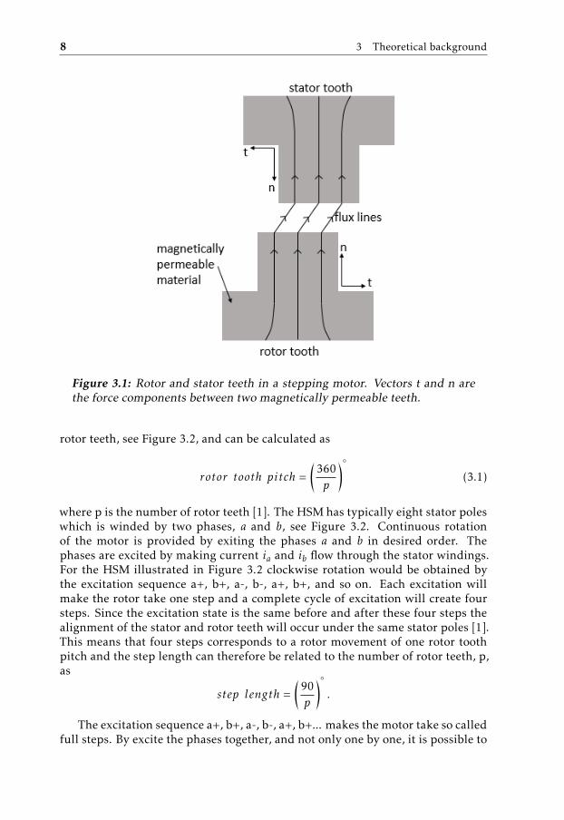
per step [16]. Stepping motors has doubly salient structure, which means thatboth the rotor and stator teeth consists of magnetically permeable material, seeFigure 3.1. As seen in the figure the magnetic flux crosses the air gap between theteeth causing a normal force n, which tries to close the air gap, and a tangentialforce t, which moves the teeth sideways. This forces will be zero as soon as themagnetic flux is removed [1].
The Hybrid Stepper Motor, HSM, has a doubly salient structure [1]. Themagnetic circuit is exited by a combination of windings on the stator, and a per-manent magnet on the rotor, see Figure 3.2. In the figure the stator poles arewounded separately. It is also possible to wound them together two and twowhich will improve the torque production [16]. The rotor in a HSM consists oftwo identical rotor stacks which are displaced axially along the rotor and in angleby one half of the rotor tooth pitch. The rotor tooth pith is the angle between two
7
8 3 Theoretical background
Figure 3.1: Rotor and stator teeth in a stepping motor. Vectors t and n arethe force components between two magnetically permeable teeth.
rotor teeth, see Figure 3.2, and can be calculated as
rotor tooth pitch =(
360p
)(3.1)
where p is the number of rotor teeth [1]. The HSM has typically eight stator poleswhich is winded by two phases, a and b, see Figure 3.2. Continuous rotationof the motor is provided by exiting the phases a and b in desired order. Thephases are excited by making current ia and ib flow through the stator windings.For the HSM illustrated in Figure 3.2 clockwise rotation would be obtained bythe excitation sequence a+, b+, a-, b-, a+, b+, and so on. Each excitation willmake the rotor take one step and a complete cycle of excitation will create foursteps. Since the excitation state is the same before and after these four steps thealignment of the stator and rotor teeth will occur under the same stator poles [1].This means that four steps corresponds to a rotor movement of one rotor toothpitch and the step length can therefore be related to the number of rotor teeth, p,as
step length =(
90p
).
The excitation sequence a+, b+, a-, b-, a+, b+... makes the motor take so calledfull steps. By excite the phases together, and not only one by one, it is possible to
3.2 Load Angle 9
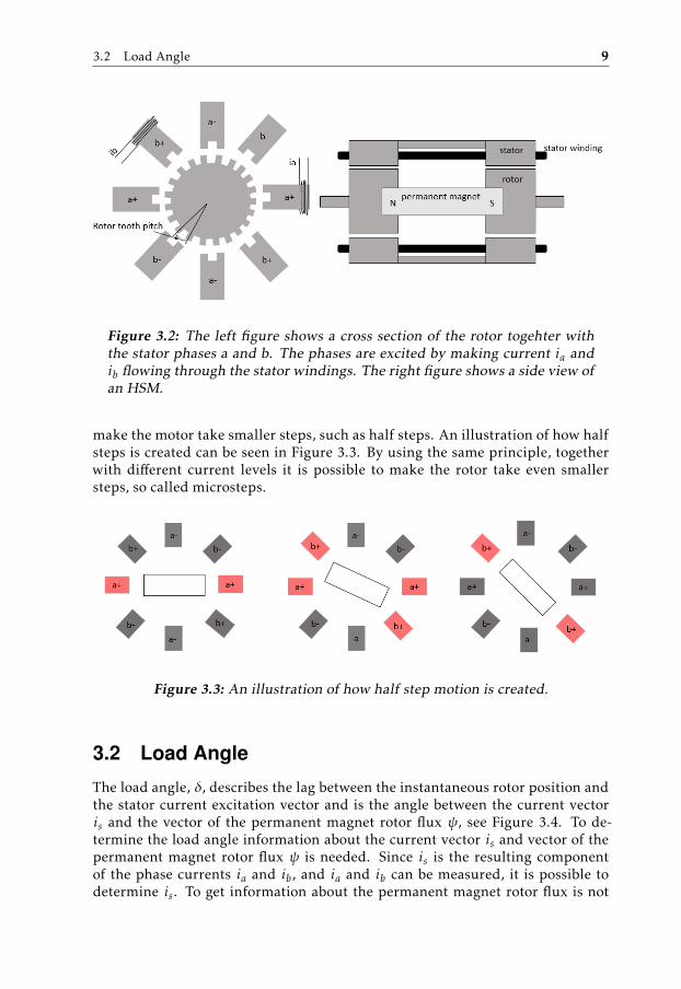
Figure 3.2: The left figure shows a cross section of the rotor togehter withthe stator phases a and b. The phases are excited by making current ia andib flowing through the stator windings. The right figure shows a side view ofan HSM.
make the motor take smaller steps, such as half steps. An illustration of how halfsteps is created can be seen in Figure 3.3. By using the same principle, togetherwith different current levels it is possible to make the rotor take even smallersteps, so called microsteps.
Figure 3.3: An illustration of how half step motion is created.
3.2 Load Angle
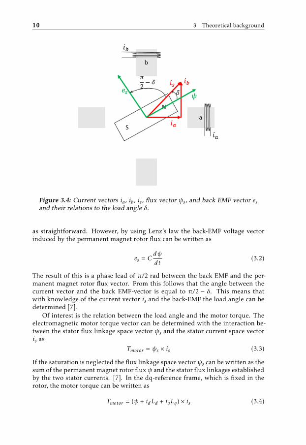
The load angle, δ, describes the lag between the instantaneous rotor position andthe stator current excitation vector and is the angle between the current vectoris and the vector of the permanent magnet rotor flux ψ, see Figure 3.4. To de-termine the load angle information about the current vector is and vector of thepermanent magnet rotor flux ψ is needed. Since is is the resulting componentof the phase currents ia and ib, and ia and ib can be measured, it is possible todetermine is. To get information about the permanent magnet rotor flux is not
10 3 Theoretical background
Figure 3.4: Current vectors ia, ib, is, flux vector ψs, and back EMF vector esand their relations to the load angle δ.
as straightforward. However, by using Lenz’s law the back-EMF voltage vectorinduced by the permanent magnet rotor flux can be written as
es = Cdψ
dt(3.2)
The result of this is a phase lead of π/2 rad between the back EMF and the per-manent magnet rotor flux vector. From this follows that the angle between thecurrent vector and the back EMF-vector is equal to π/2 − δ. This means thatwith knowledge of the current vector is and the back-EMF the load angle can bedetermined [7].
Of interest is the relation between the load angle and the motor torque. Theelectromagnetic motor torque vector can be determined with the interaction be-tween the stator flux linkage space vector ψs and the stator current space vectoris as
Tmotor = ψs × is (3.3)
If the saturation is neglected the flux linkage space vector ψs can be written as thesum of the permanent magnet rotor flux ψ and the stator flux linkages establishedby the two stator currents. [7]. In the dq-reference frame, which is fixed in therotor, the motor torque can be written as
Tmotor = (ψ + idLd + iqLq) × is (3.4)
3.3 Sliding Discrete Fourier Transform 11
The electromagnetic torque value can be written as a function of is and the loadangle δ as
Tmotor = ψissin(δ) +Ld − Lq
2i2s sin(2δ) (3.5)
In equation (3.5) the first term describes the torque generated by the interactionbetween ψ and is. The second term represent the reluctance effect due to themulti toothed rotor. As seen the two terms depend on the sine of the load anglerespectively sine of twice the load angle. This means that the relation betweenthe load angle and the generated torque should be sinusoidal. If the motor hastwo phases the maximum load angle before step loss occurs is π/2.
3.3 Sliding Discrete Fourier Transform
To determine the fundamental component of a signal, Fourier analysis can beused [6], [7]. At a discrete time instance k, the hth harmonic component Xh[k]can be written as
Xh[k] =N−1∑l=0
x[k − [N − 1] + l]e−2πhjl/N (3.6)
To be able to calculate the fundamental component, h = 1, a signal of N samplesis needed. When a new sample is available equation (3.6) updates the fundamen-tal component. To sum all measurement samples over one signal period N istime consuming. However it is possible to only add the newest sample x[n] andremove the oldest sample x[n-N]. This creates a sliding window over the signalin which the fundamental harmonic component is calculated. This operation iscalled a Sliding Discrete Fourier Transform, SDFT, [6]. The Fourier componentXh[k] at a time instance k is written as
Xh[k] = x[k − [N − 1]] + x[k − [N − 1] + 1]e−2πhj/N + x[k]e−2πhj[N−1]/N (3.7)
The previous component Xh[k − 1] is written as
Xh[k − 1] = x[k − N ] + x[k − [N − 1]]e−2πhj/N + x[k − 1]e−2πhj[N−1]/N (3.8)
Equation (3.8) can also be subtracted from equation (3.7)
Xh[k] = [Xh[k − 1] − x[k − N ]]e2πhj/N + x[k]e−2πhj[N−1]/N (3.9)
Due to the relatione2πhj/N = e−2πhj[N−1]/N (3.10)
equation (3.9) can be rewritten as
Xh[k] = [Xh[k − 1] + x[k] − x[k − N ]]e2πhj/N (3.11)
12 3 Theoretical background
3.4 Multiple linear regression
A task that often occurs when developing models is to estimate the model param-eters. The model made for the HSM will ba a model based on physical fundamen-tals and the parameters will therefore be physical [11]. One way of determiningthe model parameters are by using multiple linear regression. The general multi-ple regression model has the form
Y = β0 + β1X1 + · · · + βpXp (3.12)
where Y is the model response, X = [1, X1, · · · , Xp] are the regressors of the modeland β = [β0, · · · , βp] are unknown parameters [17]. If the values of X are specified,equation (3.12) can be written as
y = β0 + β1x1 + · · · + βpxp (3.13)
Suppose data is observed for n cases. This means that Y , X and β can be definedas
Y =
y1y2...yn
X =
1 x11 · · · x1p1 x21 · · · x2p...
......
...1 xn1 · · · xnp
β =
β0β1...βp
. (3.14)
In matrix terms (3.14) the mean function of the model response is
Y = Xβ. (3.15)
An estimation of the parameters β can be done by using ordinary least squares(OLS) estimation. The least squares estimate β of β is chosen to minimize theResidual Sum of Squares (RSS) function [17]. If yi is the true output from thesystem and xTi , i = 1 · · · n, is the ith row of X the RSS function is
RSS(β) =∑
(yi − xTi β)2 = (Y − Xβ)T (Y − Xβ). (3.16)
The OLS estimates can be found from (3.16) by differentiation with respect to βin a matrix [17]. Provided that the inverse (XTX)−1 exits, the OLS estimate isgiven by equation (3.17).
β = (XTX)−1XT Y (3.17)
3.5 Residual analysis
To determine if a model is able to explain a data set residual analysis can be used.In this thesis the residuals will be defined as the prediction error, see equation(3.18) [11].
ε(t, β) = y(t) − y(t; β) (3.18)
A good model or estimation method should yield residuals with the propertiessuch as the residuals are uncorrelated and have zero mean. If the residuals are
3.6 Extended Kalman Filter 13
correlated, it means that there are information left in the residuals that can beused in the model or in the estimation method. If the residuals does not have zeromean, it means that the result is biased. If an estimation method gives residualsthat are correlated and have zero mean this means that the estimation method canbe improved. The autocorrelation (ACF) of the residuals can be used to determineif the residuals are uncorrelated [8]. The autocorrelation of a signal for time-lagsτ is
R(τ) =E[(Xt − µ)(Xt+τ − µ)]
σ2 (3.19)
where µ is the mean and σ2 is the variance [12]. If the ACF is zero for all τ , 0the signal is not correlated.
To determine if the residual has zero mean it is possible to look at the his-tograms of the residual. A histogram is a graphical representation of the distribu-tion of the data.
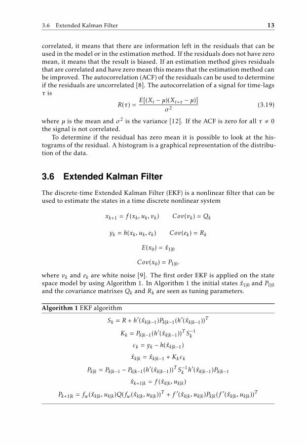
3.6 Extended Kalman Filter
The discrete-time Extended Kalman Filter (EKF) is a nonlinear filter that can beused to estimate the states in a time discrete nonlinear system
xk+1 = f (xk , uk , vk) Cov(vk) = Qk
yk = h(xk , uk , ek) Cov(ek) = Rk
E(x0) = x1|0
Cov(x0) = P1|0.
where vk and ek are white noise [9]. The first order EKF is applied on the statespace model by using Algorithm 1. In Algorithm 1 the initial states x1|0 and P1|0and the covariance matrixes Qk and Rk are seen as tuning parameters.
Algorithm 1 EKF algorithm
Sk = R + h′(xk|k−1)Pk|k−1(h′(xk|k−1))T
Kk = Pk|k−1(h′(xk|k−1))T S−1k
εk = yk − h(xk|k−1)
xk|k = xk|k−1 + Kkεk
Pk|k = Pk|k−1 − Pk|k−1(h′(xk|k−1))T S−1k h′(xk|k−1)Pk|k−1
xk+1|k = f (xk|k , uk|k)
Pk+1|k = fw(xk|k , uk|k)Q(fw(xk|k , uk|k))T + f ′(xk|k , uk|k)Pk|k(f
′(xk|k , uk|k))T
14 3 Theoretical background
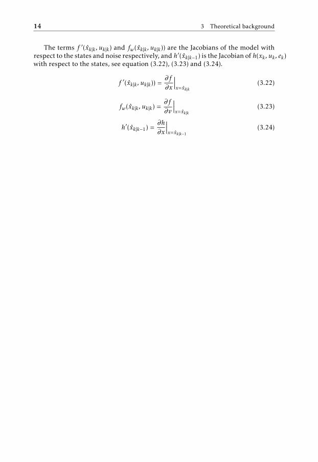
The terms f ′(xk|k , uk|k) and fw(xk|k , uk|k)) are the Jacobians of the model withrespect to the states and noise respectively, and h′(xk|k−1) is the Jacobian of h(xk , uk , ek)with respect to the states, see equation (3.22), (3.23) and (3.24).
f ′(xk|k , uk|k)) =∂f
∂x
∣∣∣∣x=xk|k
(3.22)
fw(xk|k , uk|k) =∂f
∂v
∣∣∣∣x=xk|k
(3.23)
h′(xk|k−1) =∂h∂x
∣∣∣∣x=xk|k−1
(3.24)

4Data collection
This chapter will first describe the equipment used to collect the data. I willcontinue by describing the used motor and some of its characteristics. In the endof the chapter the collected datasets and what they are used for are described.
4.1 Equipment setup
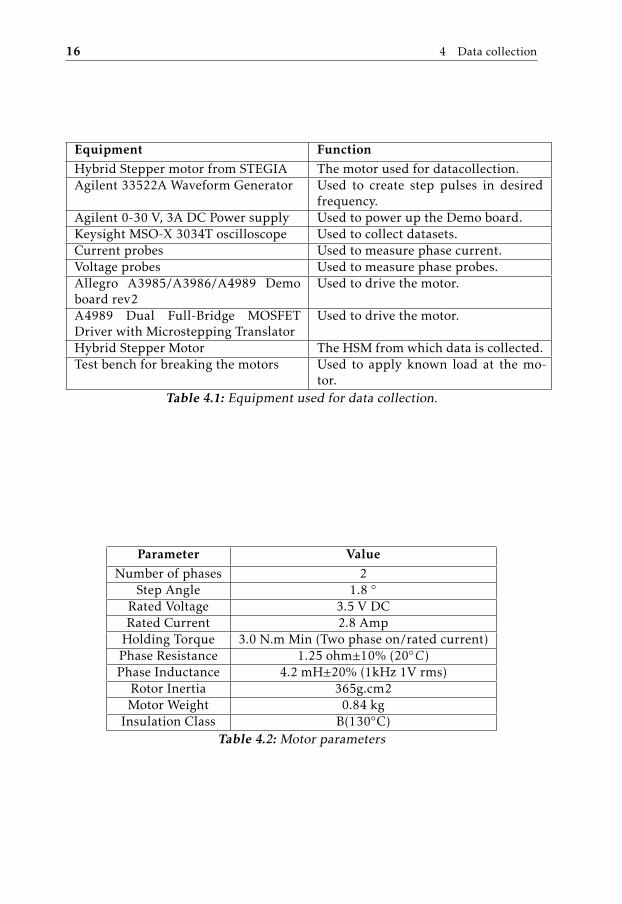
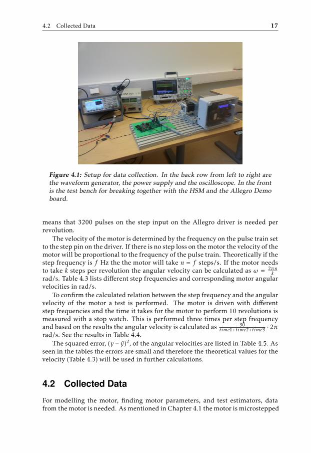
The hardware used for data collection is presented in Table 4.1, and the setupfor data collection is shown in Figure 4.1. The motor used is a Hybrid StepperMotor, HSM, see detailed description in Chapter 3. The given parameters for themotor are listed in Table 4.2.
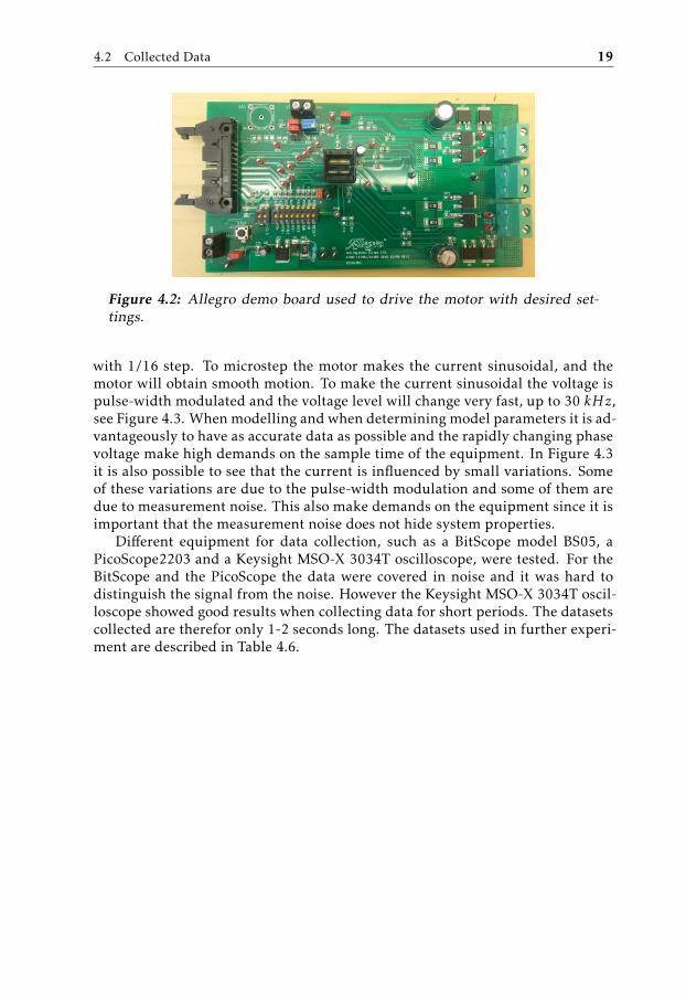
To run the motor a driver, together with a demo board from Allegro is used,see Figure 4.2. The demo board has switches which makes it possible for theuser to easy change settings [13]. To make the motor drive as smooth as possiblemixed decay mode is used together with microstepping with 1/16 step. Mixeddecay mode is a technique to obtain greater control of the phase current when itis decreasing [13]. On the driver it is also possible to set HOLD on and off. WhenHOLD is on, the motor generates as much torque as possible with the given power.The motor will take one step each time the step pin, see the pin-diagram in [13],goes high. To be able to create a motion a pulse train will be applied to the steppin. To perform this pulse train a waveform generator is used, with which it ispossible to set a desired frequency. For collecting data it is of interest to knowthe motor load. With a test bench, which is used to break the motor, it is possibleto set the load torque between 0 and 6 Nm.
The motor has a step angle of 1.8 . According to equation (3.1) this impliesthat the number of rotor teeth, p, are 50. When driving in full step the motorwill perform 360
1.8 = 200 steps per revolution. Since the motor is microsteppedwith 1/16 step the motor will perform 200 · 16 = 3200 steps per revolution. This
15
16 4 Data collection
Equipment FunctionHybrid Stepper motor from STEGIA The motor used for datacollection.Agilent 33522A Waveform Generator Used to create step pulses in desired
frequency.Agilent 0-30 V, 3A DC Power supply Used to power up the Demo board.Keysight MSO-X 3034T oscilloscope Used to collect datasets.Current probes Used to measure phase current.Voltage probes Used to measure phase probes.Allegro A3985/A3986/A4989 Demoboard rev2
Used to drive the motor.
A4989 Dual Full-Bridge MOSFETDriver with Microstepping Translator
Used to drive the motor.
Hybrid Stepper Motor The HSM from which data is collected.Test bench for breaking the motors Used to apply known load at the mo-
tor.Table 4.1: Equipment used for data collection.
Parameter ValueNumber of phases 2
Step Angle 1.8
Rated Voltage 3.5 V DCRated Current 2.8 Amp
Holding Torque 3.0 N.m Min (Two phase on/rated current)Phase Resistance 1.25 ohm±10% (20C)Phase Inductance 4.2 mH±20% (1kHz 1V rms)
Rotor Inertia 365g.cm2Motor Weight 0.84 kg
Insulation Class B(130C)Table 4.2: Motor parameters
4.2 Collected Data 17
Figure 4.1: Setup for data collection. In the back row from left to right arethe waveform generator, the power supply and the oscilloscope. In the frontis the test bench for breaking together with the HSM and the Allegro Demoboard.
means that 3200 pulses on the step input on the Allegro driver is needed perrevolution.
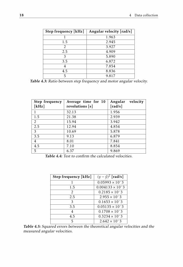
The velocity of the motor is determined by the frequency on the pulse train setto the step pin on the driver. If there is no step loss on the motor the velocity of themotor will be proportional to the frequency of the pulse train. Theoretically if thestep frequency is f Hz the the motor will take n = f steps/s. If the motor needsto take k steps per revolution the angular velocity can be calculated as ω = 2πn
krad/s. Table 4.3 lists different step frequencies and corresponding motor angularvelocities in rad/s.
To confirm the calculated relation between the step frequency and the angularvelocity of the motor a test is performed. The motor is driven with differentstep frequencies and the time it takes for the motor to perform 10 revolutions ismeasured with a stop watch. This is performed three times per step frequencyand based on the results the angular velocity is calculated as 30
time1+time2+time3 · 2πrad/s. See the results in Table 4.4.
The squared error, (y − y)2, of the angular velocities are listed in Table 4.5. Asseen in the tables the errors are small and therefore the theoretical values for thevelocity (Table 4.3) will be used in further calculations.
4.2 Collected Data
For modelling the motor, finding motor parameters, and test estimators, datafrom the motor is needed. As mentioned in Chapter 4.1 the motor is microstepped
18 4 Data collection
Step frequency [kHz] Angular velocity [rad/s]1 1.963
1.5 2.9452 3.927
2.5 4.9093 5.890
3.5 6.8724 7.854
4.5 8.8365 9.817
Table 4.3: Ratio between step frequency and motor angular velocity.
Step frequency[kHz]
Average time for 10revolutions [s]
Angular velocity[rad/s]
1 32.13 1.9561.5 21.38 2.9392 15.94 3.9422.5 12.94 4.8543 10.69 5.8783.5 9.13 6.8794 8.01 7.8414.5 7.10 8.8545 6.37 9.869
Table 4.4: Test to confirm the calculated velocities.
Step frequency [kHz] (y − y)2 [rad/s]1 0.05993 × 10⁻³
1.5 0.004133 × 10⁻³² 0.2185 × 10⁻³
2.5 2.955 × 10⁻³³ 0.1653 × 10⁻³
3.5 0.05135 × 10⁻³⁴ 0.1708 × 10⁻³
4.5 0.3234 × 10⁻³⁵ 2.642 × 10⁻³
Table 4.5: Squared errors between the theoretical angular velocities and themeasured angular velocities.
4.2 Collected Data 19
Figure 4.2: Allegro demo board used to drive the motor with desired set-tings.
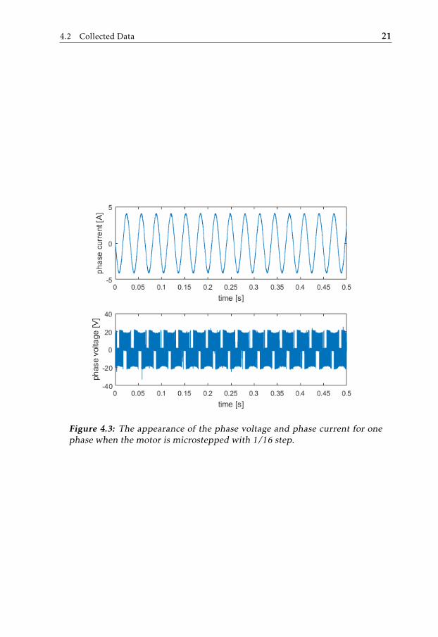
with 1/16 step. To microstep the motor makes the current sinusoidal, and themotor will obtain smooth motion. To make the current sinusoidal the voltage ispulse-width modulated and the voltage level will change very fast, up to 30 kHz,see Figure 4.3. When modelling and when determining model parameters it is ad-vantageously to have as accurate data as possible and the rapidly changing phasevoltage make high demands on the sample time of the equipment. In Figure 4.3it is also possible to see that the current is influenced by small variations. Someof these variations are due to the pulse-width modulation and some of them aredue to measurement noise. This also make demands on the equipment since it isimportant that the measurement noise does not hide system properties.
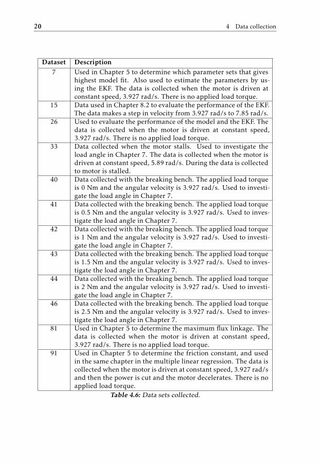
Different equipment for data collection, such as a BitScope model BS05, aPicoScope2203 and a Keysight MSO-X 3034T oscilloscope, were tested. For theBitScope and the PicoScope the data were covered in noise and it was hard todistinguish the signal from the noise. However the Keysight MSO-X 3034T oscil-loscope showed good results when collecting data for short periods. The datasetscollected are therefor only 1-2 seconds long. The datasets used in further experi-ment are described in Table 4.6.
20 4 Data collection
Dataset Description7 Used in Chapter 5 to determine which parameter sets that gives
highest model fit. Also used to estimate the parameters by us-ing the EKF. The data is collected when the motor is driven atconstant speed, 3.927 rad/s. There is no applied load torque.
15 Data used in Chapter 8.2 to evaluate the performance of the EKF.The data makes a step in velocity from 3.927 rad/s to 7.85 rad/s.
26 Used to evaluate the performance of the model and the EKF. Thedata is collected when the motor is driven at constant speed,3.927 rad/s. There is no applied load torque.
33 Data collected when the motor stalls. Used to investigate theload angle in Chapter 7. The data is collected when the motor isdriven at constant speed, 5.89 rad/s. During the data is collectedto motor is stalled.
40 Data collected with the breaking bench. The applied load torqueis 0 Nm and the angular velocity is 3.927 rad/s. Used to investi-gate the load angle in Chapter 7.
41 Data collected with the breaking bench. The applied load torqueis 0.5 Nm and the angular velocity is 3.927 rad/s. Used to inves-tigate the load angle in Chapter 7.
42 Data collected with the breaking bench. The applied load torqueis 1 Nm and the angular velocity is 3.927 rad/s. Used to investi-gate the load angle in Chapter 7.
43 Data collected with the breaking bench. The applied load torqueis 1.5 Nm and the angular velocity is 3.927 rad/s. Used to inves-tigate the load angle in Chapter 7.
44 Data collected with the breaking bench. The applied load torqueis 2 Nm and the angular velocity is 3.927 rad/s. Used to investi-gate the load angle in Chapter 7.
46 Data collected with the breaking bench. The applied load torqueis 2.5 Nm and the angular velocity is 3.927 rad/s. Used to inves-tigate the load angle in Chapter 7.
81 Used in Chapter 5 to determine the maximum flux linkage. Thedata is collected when the motor is driven at constant speed,3.927 rad/s. There is no applied load torque.
91 Used in Chapter 5 to determine the friction constant, and usedin the same chapter in the multiple linear regression. The data iscollected when the motor is driven at constant speed, 3.927 rad/sand then the power is cut and the motor decelerates. There is noapplied load torque.
Table 4.6: Data sets collected.
4.2 Collected Data 21
Figure 4.3: The appearance of the phase voltage and phase current for onephase when the motor is microstepped with 1/16 step.

5Modeling
This chapter will present a model of an HSM based on fundamental electrical andmechanical equations. The model will be implemented in Simulink and used infurther investigations.
5.1 Motor model
The motor model used in the thesis is divided in an electrical and a mechanicalpart. An overview of the model and its parameters can be seen in figure 5.1. Theback EMF induced in coil a is given by
ea = ωpψm sin(pθ) (5.1)
where
ω - the rotor angular velocity, [rad/s]
p - the rotor teeth number
ψm - the maximum flux linkage, [Vs/rad]
θ - the angular position of the rotor, [rad]
Similarly, the back EMF induced in coil b is given by
eb = ωpψm sin(pθ − λ) (5.2)
where λ is the phase angle [15]. For a motor with two stator phases λ = π2 and
equation (5.3) can therefore be rewritten as
eb = −ωpψm cos(pθ) (5.3)
23
24 5 Modeling
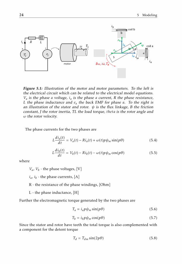
Figure 5.1: Illustration of the motor and motor parameters. To the left isthe electrical circuit which can be related to the electrical model equations.Va is the phase a voltage, ia is the phase a current, R the phase resistance,L the phase inductance and ea the back EMF for phase a. To the right isan illustration of the stator and rotor. ψ is the flux linkage, B the frictionconstant, J the rotor inertia, TL the load torque, theta is the rotor angle andω the rotor velocity.
The phase currents for the two phases are
Ldia(t)dt
= Va(t) − Ria(t) + ω(t)pψm sin(pθ) (5.4)
Ldib(t)dt
= Vb(t) − Rib(t) − ω(t)pψm cos(pθ) (5.5)
where
Va, Vb - the phase voltages, [V]
ia, ib - the phase currents, [A]
R - the resistance of the phase windings, [Ohm]
L - the phase inductance, [H]
Further the electromagnetic torque generated by the two phases are
Ta = iapψm sin(pθ) (5.6)
Tb = ibpψm cos(pθ) (5.7)
Since the stator and rotor have teeth the total torque is also complemented witha component for the detent torque
Td = Tdm sin(2pθ) (5.8)
5.1 Motor model 25
where Tdm is the maximum detent torque [15]. The electromagnetic torque of themotor is the sum of the phase torques and the detent torque
Te = −Ta − Tb − Td = −iapψm sin(pθ) − ibpψm cos(pθ) − Tdm sin(2pθ) (5.9)
The rotor motion can now be described as
Jdω(t)dt
= Te(t) − TL − Bω(t) (5.10)
where
J - the rotor inertia [kg m2]
TL - the load torque [Nm]
B - Friction constant [Nms/rad]
By substituting the equation (5.9) into equation (5.10) the total equation describ-ing the motion is obtained.
Jdω(t)dt
= −iapψm sin(pθ) − ibpψm cos(pθ) − Tdm sin(2pθ) − TL − Bω(t) (5.11a)
dθdt
= ω (5.11b)

6Determination of unknown motor
parameters
The unknown parameters needed for the model are the detent torque Tdm, thefriction constant B and the maximum flux linkage ψm. In this section three differ-ent ways to determine the motor parameters will be presented.
6.1 Determination of parameters individually
This section will explain how the parameters can be determined one by one. Thedetent torque Tdm is determined by using a torque wrench and the friction con-stant B and the maximum flux linkage ψm is determined by using linear regres-sion.
6.1.1 Detent torque
The detent torque, Tdm can be determined by help of a torque wrench when themotor phases are unexcited. By using this method the detent torque was deter-mined to Tdm = 0.1Nm.
6.1.2 Friction constant
To determine B the equation (5.11a) can be used. The motor is driven at a con-stant speed with no load and after a while the power is cut and data are collectedduring the time the motor decelerates. From the time the power is cut the phasecurrents, ia and ib, are zero and the remaining parts of equation (5.11a) is there-fore
Jdω(t)dt
= −Tdm sin(2pθ) − Bω(t) (6.1)
27
28 6 Determination of unknown motor parameters
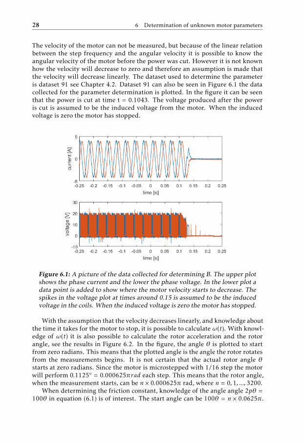
The velocity of the motor can not be measured, but because of the linear relationbetween the step frequency and the angular velocity it is possible to know theangular velocity of the motor before the power was cut. However it is not knownhow the velocity will decrease to zero and therefore an assumption is made thatthe velocity will decrease linearly. The dataset used to determine the parameteris dataset 91 see Chapter 4.2. Dataset 91 can also be seen in Figure 6.1 the datacollected for the parameter determination is plotted. In the figure it can be seenthat the power is cut at time t = 0.1043. The voltage produced after the poweris cut is assumed to be the induced voltage from the motor. When the inducedvoltage is zero the motor has stopped.
Figure 6.1: A picture of the data collected for determining B. The upper plotshows the phase current and the lower the phase voltage. In the lower plot adata point is added to show where the motor velocity starts to decrease. Thespikes in the voltage plot at times around 0.15 is assumed to be the inducedvoltage in the coils. When the induced voltage is zero the motor has stopped.
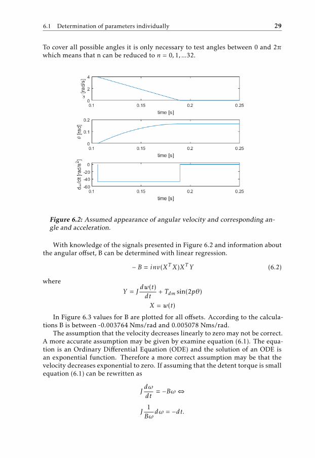
With the assumption that the velocity decreases linearly, and knowledge aboutthe time it takes for the motor to stop, it is possible to calculate ω(t). With knowl-edge of ω(t) it is also possible to calculate the rotor acceleration and the rotorangle, see the results in Figure 6.2. In the figure, the angle θ is plotted to startfrom zero radians. This means that the plotted angle is the angle the rotor rotatesfrom the measurements begins. It is not certain that the actual rotor angle θstarts at zero radians. Since the motor is microstepped with 1/16 step the motorwill perform 0.1125 = 0.000625πrad each step. This means that the rotor angle,when the measurement starts, can be n × 0.000625π rad, where n = 0, 1, ..., 3200.
When determining the friction constant, knowledge of the angle angle 2pθ =100θ in equation (6.1) is of interest. The start angle can be 100θ = n × 0.0625π.
6.1 Determination of parameters individually 29
To cover all possible angles it is only necessary to test angles between 0 and 2πwhich means that n can be reduced to n = 0, 1, ...32.
Figure 6.2: Assumed appearance of angular velocity and corresponding an-gle and acceleration.
With knowledge of the signals presented in Figure 6.2 and information aboutthe angular offset, B can be determined with linear regression.
− B = inv(XTX)XT Y (6.2)
where
Y = Jdw(t)dt
+ Tdm sin(2pθ)
X = w(t)
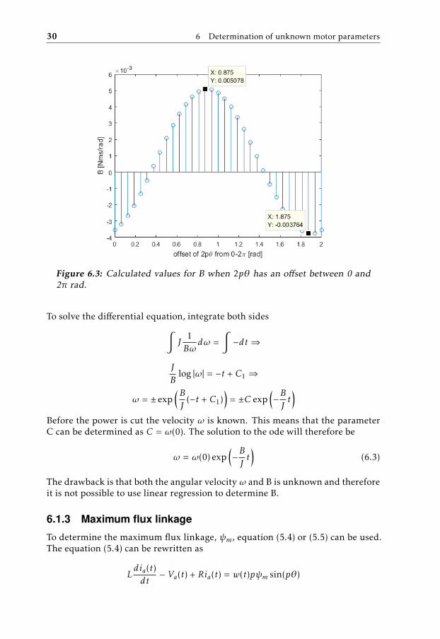
In Figure 6.3 values for B are plotted for all offsets. According to the calcula-tions B is between -0.003764 Nms/rad and 0.005078 Nms/rad.
The assumption that the velocity decreases linearly to zero may not be correct.A more accurate assumption may be given by examine equation (6.1). The equa-tion is an Ordinary Differential Equation (ODE) and the solution of an ODE isan exponential function. Therefore a more correct assumption may be that thevelocity decreases exponential to zero. If assuming that the detent torque is smallequation (6.1) can be rewritten as
Jdωdt
= −Bω⇔
J1Bω
dω = −dt.
30 6 Determination of unknown motor parameters
Figure 6.3: Calculated values for B when 2pθ has an offset between 0 and2π rad.
To solve the differential equation, integrate both sides∫J
1Bω
dω =∫−dt ⇒
JB
log |ω| = −t + C1 ⇒
ω = ± exp(BJ
(−t + C1))
= ±C exp(−BJt)
Before the power is cut the velocity ω is known. This means that the parameterC can be determined as C = ω(0). The solution to the ode will therefore be
ω = ω(0) exp(−BJt)
(6.3)
The drawback is that both the angular velocity ω and B is unknown and thereforeit is not possible to use linear regression to determine B.
6.1.3 Maximum flux linkage
To determine the maximum flux linkage, ψm, equation (5.4) or (5.5) can be used.The equation (5.4) can be rewritten as
Ldia(t)dt
− Va(t) + Ria(t) = w(t)pψm sin(pθ)
6.1 Determination of parameters individually 31
The data needed can be obtained by letting the motor drive with constant velocityω and measure the phase voltage and phase current of one phase, see dataset81 in Chapter 4.2. Since all parameters in equation (5.4) except the maximumflux linkage is known, or can be measured, the maximum flux linkage can bedetermined by linear regression where
Y = Ldia(t)dt
− Va(t) + Ria(t)
X = w(t)p sin(pθ).
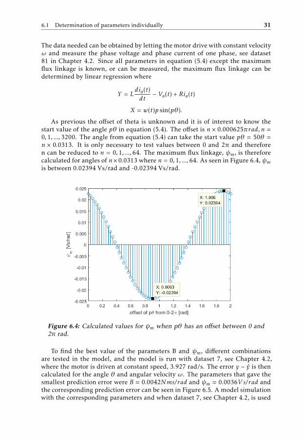
As previous the offset of theta is unknown and it is of interest to know thestart value of the angle pθ in equation (5.4). The offset is n × 0.000625πrad, n =0, 1, ..., 3200. The angle from equation (5.4) can take the start value pθ = 50θ =n × 0.0313. It is only necessary to test values between 0 and 2π and thereforen can be reduced to n = 0, 1, ..., 64. The maximum flux linkage, ψm, is thereforecalculated for angles of n×0.0313 where n = 0, 1, ..., 64. As seen in Figure 6.4, ψmis between 0.02394 Vs/rad and -0.02394 Vs/rad.
Figure 6.4: Calculated values for ψm when pθ has an offset between 0 and2π rad.
To find the best value of the parameters B and ψm, different combinationsare tested in the model, and the model is run with dataset 7, see Chapter 4.2,where the motor is driven at constant speed, 3.927 rad/s. The error y − y is thencalculated for the angle θ and angular velocity ω. The parameters that gave thesmallest prediction error were B = 0.0042Nms/rad and ψm = 0.0036V s/rad andthe corresponding prediction error can be seen in Figure 6.5. A model simulationwith the corresponding parameters and when dataset 7, see Chapter 4.2, is used
32 6 Determination of unknown motor parameters
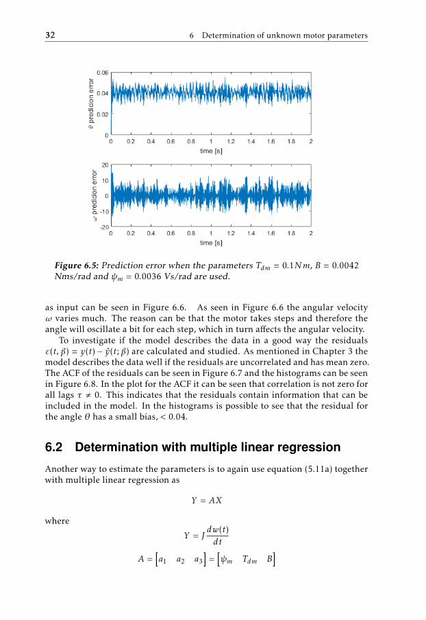
Figure 6.5: Prediction error when the parameters Tdm = 0.1Nm, B = 0.0042Nms/rad and ψm = 0.0036 Vs/rad are used.
as input can be seen in Figure 6.6. As seen in Figure 6.6 the angular velocityω varies much. The reason can be that the motor takes steps and therefore theangle will oscillate a bit for each step, which in turn affects the angular velocity.
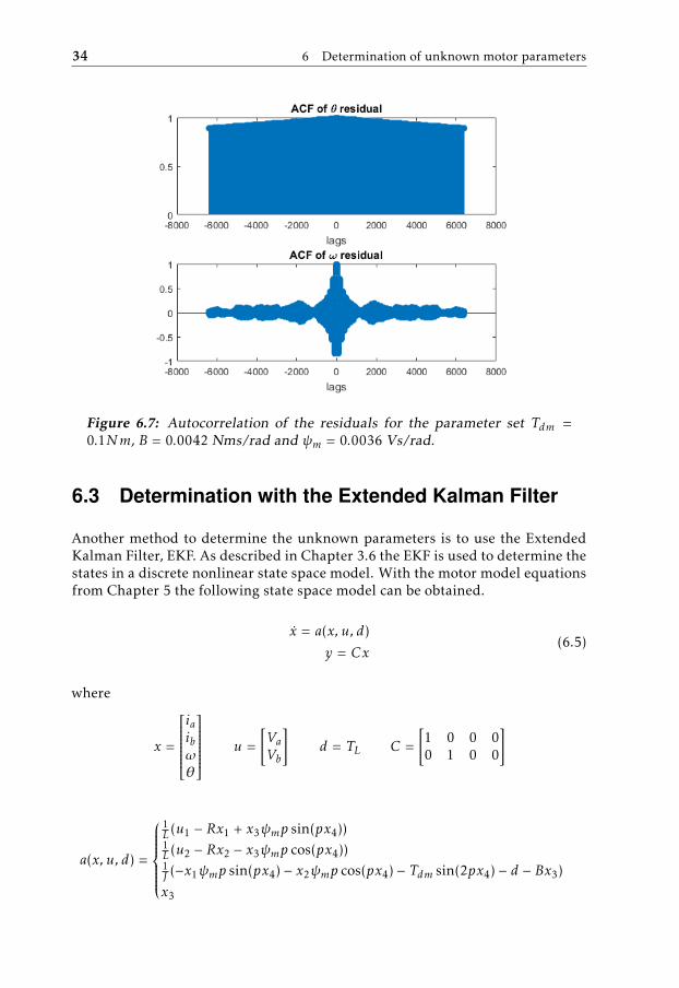
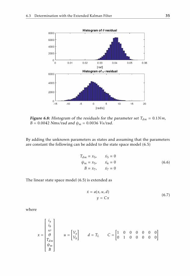
To investigate if the model describes the data in a good way the residualsε(t, β) = y(t) − y(t; β) are calculated and studied. As mentioned in Chapter 3 themodel describes the data well if the residuals are uncorrelated and has mean zero.The ACF of the residuals can be seen in Figure 6.7 and the histograms can be seenin Figure 6.8. In the plot for the ACF it can be seen that correlation is not zero forall lags τ , 0. This indicates that the residuals contain information that can beincluded in the model. In the histograms is possible to see that the residual forthe angle θ has a small bias, < 0.04.
6.2 Determination with multiple linear regression
Another way to estimate the parameters is to again use equation (5.11a) togetherwith multiple linear regression as
Y = AX
where
Y = Jdw(t)dt
A =[a1 a2 a3
]=
[ψm Tdm B
]
6.2 Determination with multiple linear regression 33
.
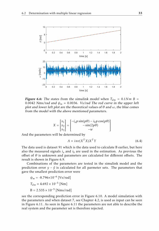
Figure 6.6: The states from the simulink model when Tdm = 0.1Nm B =0.0042 Nms/rad and ψm = 0.0036. Vs/rad The red curve in the upper leftplot and lower left plot are the theoretical values of θ and ω, the blue comesfrom the model with the above mentioned parameters.
X =
x1x2x3
=
−iap sin(pθ) − ibp cos(pθ)− sin(2pθ)−w
And the parameters will be determined by
A = inv(XTX)XT Y (6.4)
The data used is dataset 91 which is the data used to calculate B earlier, but herealso the measured signals ia and ib are used in the estimation. As previous theoffset of θ is unknown and parameters are calculated for different offsets. Theresult is shown in Figure 6.9.
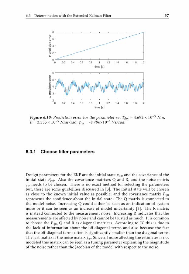
Combinations of the parameters are tested in the simulink model and theprediction error y − y is calculated for all parmeter sets. The parameters thatgave the smallest prediction error were
ψm = -8.796×10⁻⁶ [Vs/rad]
Tdm = 4.692 × 10⁻⁵ [Nm]
B = 2.535 × 10⁻⁵ [Nms/rad]
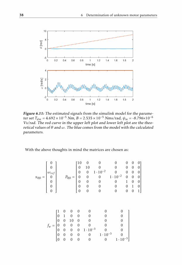
see the corresponding prediction error in Figure 6.10. A model simulation withthe parameters and when dataset 7, see Chapter 4.2, is used as input can be seenin Figure 6.11. As seen in figure 6.11 the parameters are not able to describe thereal system and the parameter set is therefore rejected.
34 6 Determination of unknown motor parameters
Figure 6.7: Autocorrelation of the residuals for the parameter set Tdm =0.1Nm, B = 0.0042 Nms/rad and ψm = 0.0036 Vs/rad.
6.3 Determination with the Extended Kalman Filter
Another method to determine the unknown parameters is to use the ExtendedKalman Filter, EKF. As described in Chapter 3.6 the EKF is used to determine thestates in a discrete nonlinear state space model. With the motor model equationsfrom Chapter 5 the following state space model can be obtained.
x = a(x, u, d)
y = Cx(6.5)
where
x =
iaibωθ
u =[VaVb
]d = TL C =
[1 0 0 00 1 0 0
]
a(x, u, d) =
1L (u1 − Rx1 + x3ψmp sin(px4))1L (u2 − Rx2 − x3ψmp cos(px4))1J (−x1ψmp sin(px4) − x2ψmp cos(px4) − Tdm sin(2px4) − d − Bx3)x3
6.3 Determination with the Extended Kalman Filter 35
Figure 6.8: Histogram of the residuals for the parameter set Tdm = 0.1Nm,B = 0.0042 Nms/rad and ψm = 0.0036 Vs/rad.
By adding the unknown parameters as states and assuming that the parametersare constant the following can be added to the state space model (6.5)
Tdm = x5,
ψm = x5,
B = x7,
x5 = 0
x6 = 0
x7 = 0
(6.6)
The linear state space model (6.5) is extended as
x = a(x, u, d)
y = Cx(6.7)
where
x =
iaibωθTdmψmB
u =
[VaVb
]d = TL C =
[1 0 0 0 0 0 00 1 0 0 0 0 0
]
36 6 Determination of unknown motor parameters
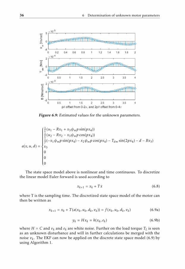
Figure 6.9: Estimated values for the unknown parameters.
a(x, u, d) =
1L (u1 − Rx1 + x3ψmp sin(px4))1L (u2 − Rx2 − x3ψmp cos(px4))1J (−x1ψmp sin(px4) − x2ψmp cos(px4) − Tdm sin(2px4) − d − Bx3)x3
000
The state space model above is nonlinear and time continuous. To discretizethe linear model Euler forward is used according to
xk+1 = xk + T x (6.8)
where T is the sampling time. The discretized state space model of the motor canthen be written as
xk+1 = xk + T (a(xk , uk , dk , vk)) = f (xk , uk , dk , vk) (6.9a)
yk = Hxk = h(xk , ek) (6.9b)
where H = C and vk and ek are white noise. Further on the load torque TL is seenas an unknown disturbance and will in further calculations be merged with thenoise vk . The EKF can now be applied on the discrete state space model (6.9) byusing Algorithm 1.
6.3 Determination with the Extended Kalman Filter 37
Figure 6.10: Prediction error for the parameter set Tdm = 4.692 × 10⁻⁵ Nm,B = 2.535 × 10⁻⁵ Nms/rad, ψm = -8.796×10⁻⁶ Vs/rad.
6.3.1 Choose filter parameters
Design parameters for the EKF are the initial state x0|0 and the covariance of theinitial state P0|0. Also the covariance matrixes Q and R, and the noise matrixfw needs to be chosen. There is no exact method for selecting the parametersbut, there are some guidelines discussed in [3]. The initial state will be chosenas close to the known initial value as possible, and the covariance matrix P0|0represents the confidence about the initial state. The Q matrix is connected tothe model noise. Increasing Q could either be seen as an indication of systemnoise or it can be seen as an increase of model uncertainty [3]. The R matrixis instead connected to the measurement noise. Increasing R indicates that themeasurements are affected by noise and cannot be trusted as much. It is commonto choose the P0|0, Q and R as diagonal matrices. According to [3] this is due tothe lack of information about the off-diagonal terms and also because the factthat the off-diagonal terms often is significantly smaller than the diagonal terms.The last matrix is the noise matrix fw. Since all noise affecting the estimates is notmodeled this matrix can be seen as a tuning parameter explaining the magnitudeof the noise rather than the Jacobian of the model with respect to the noise.
38 6 Determination of unknown motor parameters
Figure 6.11: The estimated signals from the simulink model for the parame-ter set Tdm = 4.692 × 10⁻⁵ Nm, B = 2.535 × 10⁻⁵ Nms/rad, ψm = -8.796×10⁻⁶
Vs/rad. The red curve in the upper left plot and lower left plot are the theo-retical values of θ and ω. The blue comes from the model with the calculatedparameters.
With the above thoughts in mind the matrices are chosen as:
x0|0 =
00
ωref0000
P0|0 =
10 0 0 0 0 0 00 10 0 0 0 0 00 0 1 · 10−2 0 0 0 00 0 0 1 · 10−2 0 0 00 0 0 0 1 0 00 0 0 0 0 1 00 0 0 0 0 0 1
fw =
1 0 0 0 0 0 00 1 0 0 0 0 00 0 10 0 0 0 00 0 0 0 0 0 00 0 0 0 1 · 10−3 0 00 0 0 0 0 1 · 10−3 00 0 0 0 0 0 1 · 10−3
6.4 Residual analysis 39
Q =
1 0 0 0 0 0 00 1 0 0 0 0 00 0 1 · 10−1 0 0 0 00 0 0 1 · 10−3 0 0 00 0 0 0 1 · 10−3 0 00 0 0 0 0 1 · 10−3 00 0 0 0 0 0 1 · 10−3
R =
[1 · 10−1 0
0 1 · 10−1
]
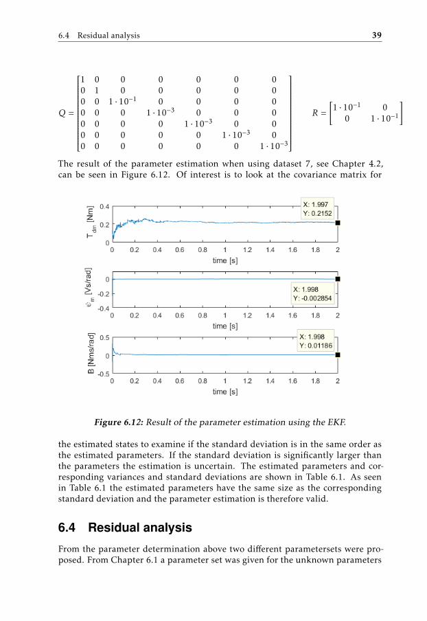
The result of the parameter estimation when using dataset 7, see Chapter 4.2,can be seen in Figure 6.12. Of interest is to look at the covariance matrix for
Figure 6.12: Result of the parameter estimation using the EKF.
the estimated states to examine if the standard deviation is in the same order asthe estimated parameters. If the standard deviation is significantly larger thanthe parameters the estimation is uncertain. The estimated parameters and cor-responding variances and standard deviations are shown in Table 6.1. As seenin Table 6.1 the estimated parameters have the same size as the correspondingstandard deviation and the parameter estimation is therefore valid.
6.4 Residual analysis
From the parameter determination above two different parametersets were pro-posed. From Chapter 6.1 a parameter set was given for the unknown parameters
40 6 Determination of unknown motor parameters
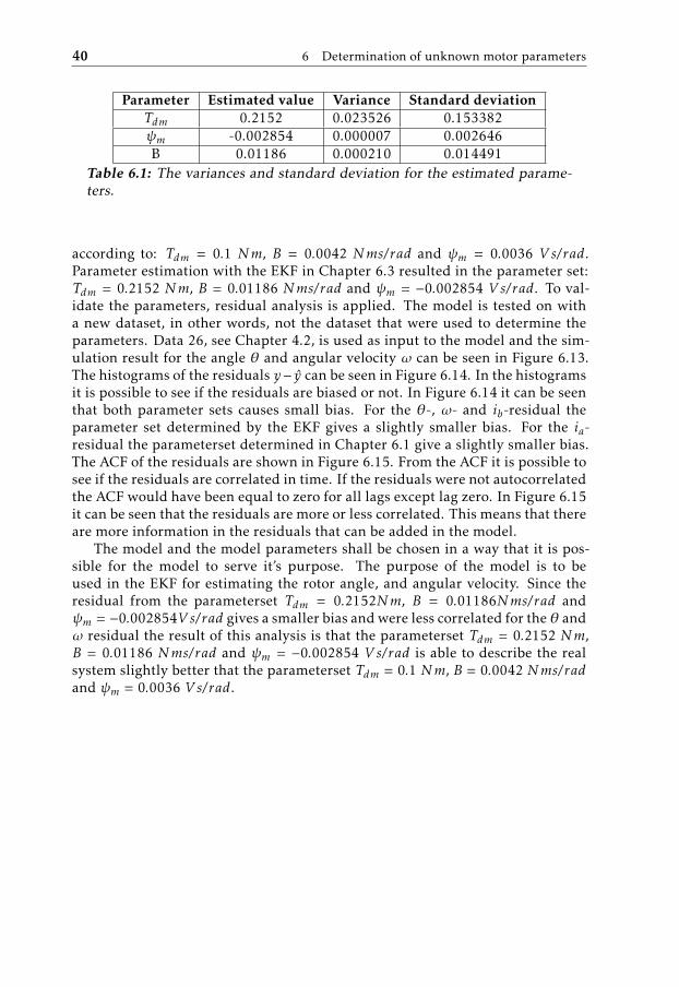
Parameter Estimated value Variance Standard deviationTdm 0.2152 0.023526 0.153382ψm -0.002854 0.000007 0.002646B 0.01186 0.000210 0.014491
Table 6.1: The variances and standard deviation for the estimated parame-ters.
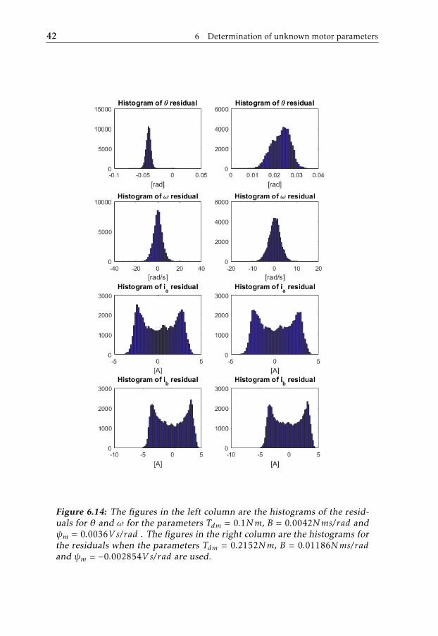
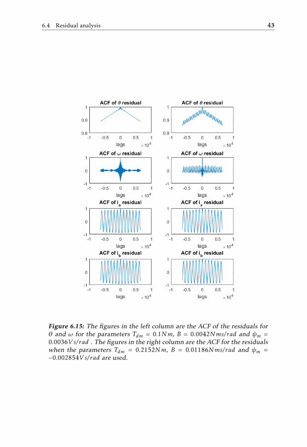
according to: Tdm = 0.1 Nm, B = 0.0042 Nms/rad and ψm = 0.0036 V s/rad.Parameter estimation with the EKF in Chapter 6.3 resulted in the parameter set:Tdm = 0.2152 Nm, B = 0.01186 Nms/rad and ψm = −0.002854 V s/rad. To val-idate the parameters, residual analysis is applied. The model is tested on witha new dataset, in other words, not the dataset that were used to determine theparameters. Data 26, see Chapter 4.2, is used as input to the model and the sim-ulation result for the angle θ and angular velocity ω can be seen in Figure 6.13.The histograms of the residuals y− y can be seen in Figure 6.14. In the histogramsit is possible to see if the residuals are biased or not. In Figure 6.14 it can be seenthat both parameter sets causes small bias. For the θ-, ω- and ib-residual theparameter set determined by the EKF gives a slightly smaller bias. For the ia-residual the parameterset determined in Chapter 6.1 give a slightly smaller bias.The ACF of the residuals are shown in Figure 6.15. From the ACF it is possible tosee if the residuals are correlated in time. If the residuals were not autocorrelatedthe ACF would have been equal to zero for all lags except lag zero. In Figure 6.15it can be seen that the residuals are more or less correlated. This means that thereare more information in the residuals that can be added in the model.
The model and the model parameters shall be chosen in a way that it is pos-sible for the model to serve it’s purpose. The purpose of the model is to beused in the EKF for estimating the rotor angle, and angular velocity. Since theresidual from the parameterset Tdm = 0.2152Nm, B = 0.01186Nms/rad andψm = −0.002854V s/rad gives a smaller bias and were less correlated for the θ andω residual the result of this analysis is that the parameterset Tdm = 0.2152 Nm,B = 0.01186 Nms/rad and ψm = −0.002854 V s/rad is able to describe the realsystem slightly better that the parameterset Tdm = 0.1 Nm, B = 0.0042 Nms/radand ψm = 0.0036 V s/rad.
6.4 Residual analysis 41
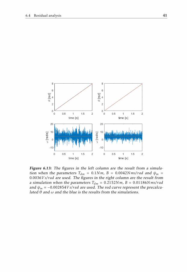
Figure 6.13: The figures in the left column are the result from a simula-tion when the parameters Tdm = 0.1Nm, B = 0.0042Nms/rad and ψm =0.0036V s/rad are used. The figures in the right column are the result froma simulation when the parameters Tdm = 0.2152Nm, B = 0.01186Nms/radand ψm = −0.002854V s/rad are used. The red curve represent the precalcu-lated θ and ω and the blue is the results from the simulations.
42 6 Determination of unknown motor parameters
Figure 6.14: The figures in the left column are the histograms of the resid-uals for θ and ω for the parameters Tdm = 0.1Nm, B = 0.0042Nms/rad andψm = 0.0036V s/rad . The figures in the right column are the histograms forthe residuals when the parameters Tdm = 0.2152Nm, B = 0.01186Nms/radand ψm = −0.002854V s/rad are used.
6.4 Residual analysis 43
Figure 6.15: The figures in the left column are the ACF of the residuals forθ and ω for the parameters Tdm = 0.1Nm, B = 0.0042Nms/rad and ψm =0.0036V s/rad . The figures in the right column are the ACF for the residualswhen the parameters Tdm = 0.2152Nm, B = 0.01186Nms/rad and ψm =−0.002854V s/rad are used.

7Estimations
This chapter will describe the estimation methods used in this thesis. In the firstsection the Extended Kalman Filter is implemented to estimate the rotor angleand rotor position. In the next section the load angle estimation is described andimplemented.
7.1 Extended Kalman Filter
An Extended Kalman Filter (EKF) can be used to estimate the rotor angular veloc-ity and the angle the rotor has rotated from the estimation started. As describedin Chapter 3.6 the EKF is used to determine the states in a discrete nonlinear statespace model. With the motor model equations from Chapter 5 the following statespace model can be obtained.
x = a(x, u, d)
y = Cx(7.1)
where
x =
iaibωθ
u =[VaVb
]d = TL C =
[1 0 0 00 1 0 0
]
a(x, u, d) =
1L (u1 − Rx1 + x3ψmp sin(px4))1L (u2 − Rx2 − x3ψmp cos(px4))1J (−x1ψmp sin(px4) − x2ψmp cos(px4) − Tdm sin(2px4) − d − Bx3)x3
45
46 7 Estimations
The state space model above is nonlinear and time continuous. To discretize thelinear model Euler forward is used according to
xk+1 = xk + T x (7.2)
where T is the sampling time. The discretized state space model of the motor canthen be written as
xk+1 = xk + T (a(xk , uk , dk , vk)) = f (xk , uk , dk , vk) (7.3a)
yk = Hxk = h(xk , ek) (7.3b)
where H = C and vk and ek are white noise. Further on the load torque TL is seenas an unknown disturbance and will in further calculations be merged with thenoise vk . The EKF can now be applied on the discrete state space model (7.3).The first order EKF is applied on the state space model by using Algorithm 1.
As described in Chapter 6.3.1, design parameters for the EKF are the initialstate x0|0, the covariance of the initial state P0|0 and the covariance matrixes Qand R, and the noise matrix fw. By using the guidelines described in Chapter6.3.1, the matrices are chosen as:
x0|0 =
00
ωref0
P0|0 =
5 0 0 00 5 0 00 0 1 · 10−2 00 0 0 6
fw =
1 0 0 00 1 0 00 0 10 00 0 0 0
Q =
1 0 0 00 1 0 00 0 1 · 10−1 00 0 0 1 · 10−3
R =[1 00 1
]
7.2 Load angle estimation
To get knowledge about the load torque [7] proposes to determine the load angle,see description in Chapter 3.2. As mentioned in Chapter 3.2 the load angle canbe determined by knowledge of the phase current and the back EMF. The currentvector is can be measured leaving only determining of the back EMF.
To estimate the back EMF equation (5.4), describing the electrical relations inthe stator phase, can be used. The equation can be rewritten as:
es = us − Lsdisdt− Rsis (7.4)
One possibility to estimate the back EMF is by solving equation (7.4), but sincethe current is a noisy signal it is not recommended. Instead the authors in [7]suggests to write equation (7.4) in the frequency domain.
Es(jω1) = Us(jω1) − jω1LsIs(jω1) − RsIs(jω1) (7.5)
7.2 Load angle estimation 47
where ω1 is the fundamental frequency [7]. To determine ω1, the fundamentalvoltage Us1 and fundamental current Is1 authors in [7] suggests to use the SDFT,see Chapter 3.3. With knowledge of the back EMF the load angle can be deter-mined according to
δ =π2− (∠(Es1 ) − ∠(Is1 )) (7.6)
The data used for calculating the load angle are dataset 33, 40, 41, 42, 43, 44and 46, which is data collected with the breaking bench for load torques between0-2.5 Nm, see Chapter 4.2. The datasets contains of collected phase voltages andphase currents for the two phases respectively.
To obtain the current vector is and the voltage vector us the phase currents iaand ib respective the phase voltages ua and ub are added together according to
is = ia + jib (7.7)
us = ua + jub (7.8)
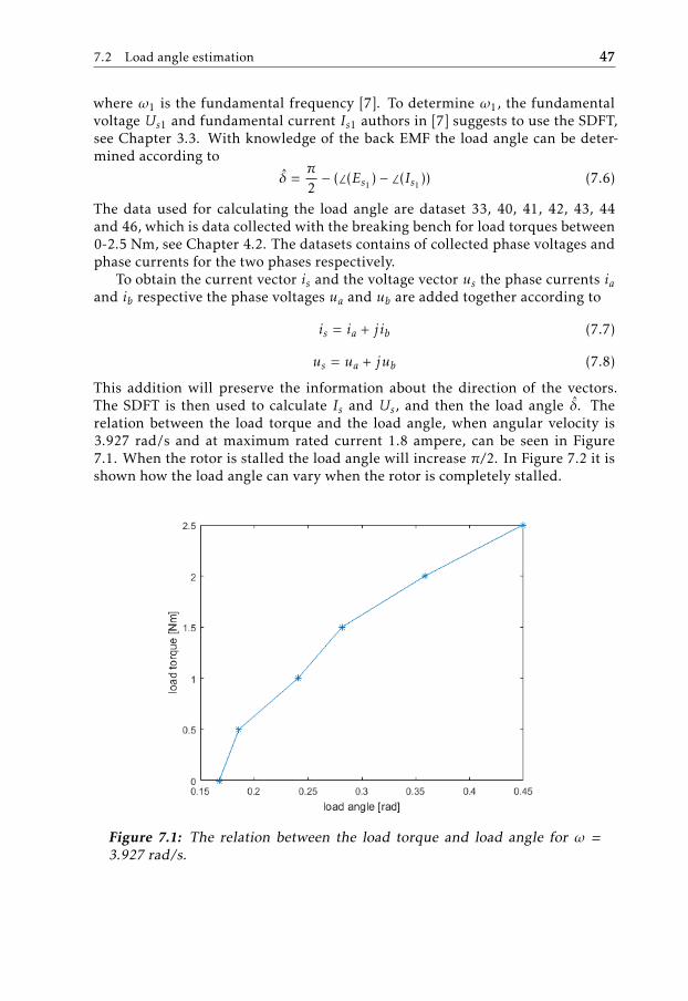
This addition will preserve the information about the direction of the vectors.The SDFT is then used to calculate Is and Us, and then the load angle δ. Therelation between the load torque and the load angle, when angular velocity is3.927 rad/s and at maximum rated current 1.8 ampere, can be seen in Figure7.1. When the rotor is stalled the load angle will increase π/2. In Figure 7.2 it isshown how the load angle can vary when the rotor is completely stalled.
Figure 7.1: The relation between the load torque and load angle for ω =3.927 rad/s.
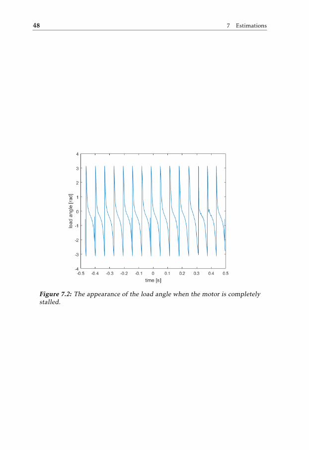
48 7 Estimations
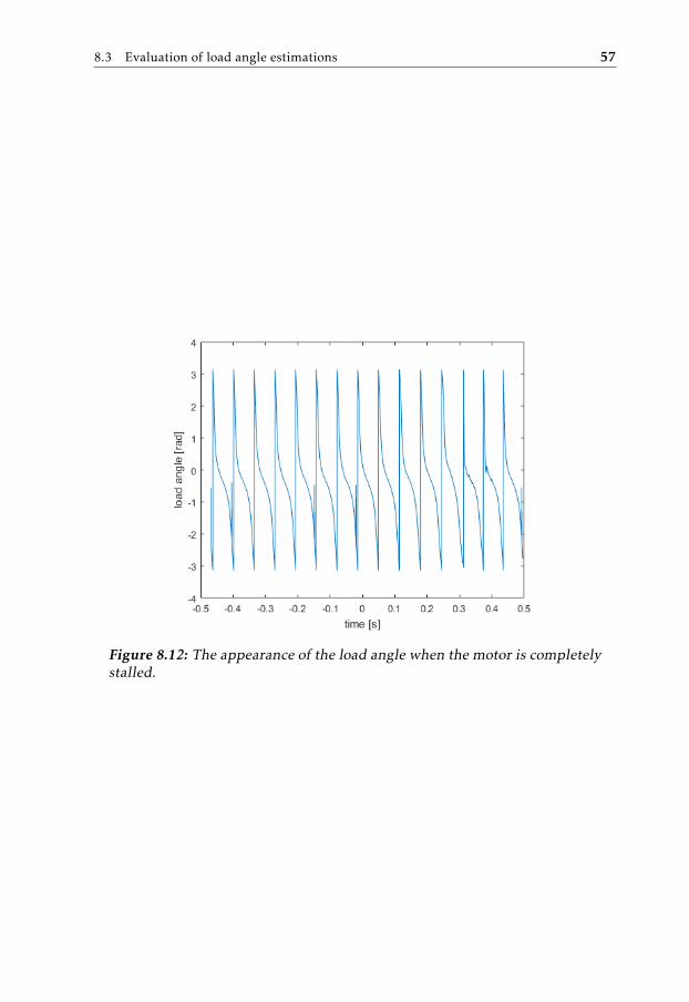
Figure 7.2: The appearance of the load angle when the motor is completelystalled.
8Results
In this chapter the results from this thesis work will be presented. In Section8.1 the model together with the determined parameters will be evaluated fordifferent datasets. The model is used in the EKF to estimate the rotor angle andangular velocity. The results from this estimations is presented in section 8.2.Finally an evaluation of the load angle estimations is presented in section 8.3.
8.1 Evaluation of model and model parameters
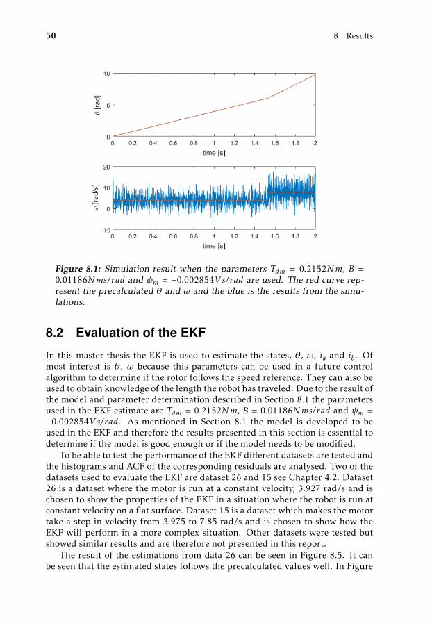
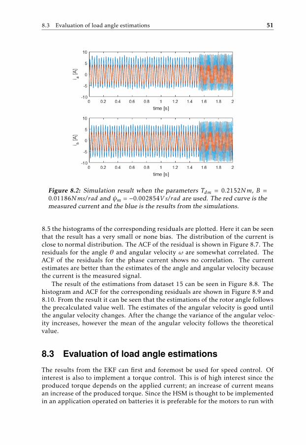
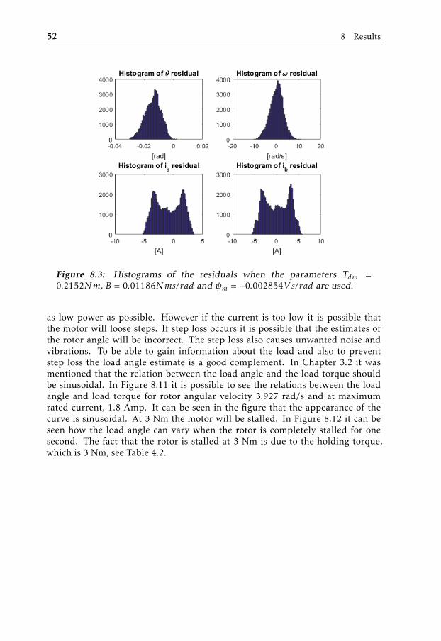
From Chapter 6 it was determined that the parameterset Tdm = 0.2152Nm, B =0.01186Nms/rad and ψm = −0.002854V s/rad, which was determined by the EKF,were the best parameterset for the model. To evaluate the model it is tested onwith a new dataset, in other words, not the dataset that were used to determinethe parameters. The dataset used will be dataset 15, see Chapter 4.2. Dataset15 is a dataset where the motor will take a step in velocity from 3.927 rad/s to7.854 rad/s and is used to see how the model will perform in a more difficultenvironment. In Figure 8.1 it is possible to see that the model is able to followthe theoretical angle well when dataset 15 is used. The estimations of the velocityis oscillating around the theoretical value, but the mean is close to the theoreticalvalue. In Figure 8.2 the current from the model can be seen. The frequency ofthe current is able to follow the measured but the amplitude is to high. Also theresiduals y − y are studied. The histograms of the residuals can be seen in Figure8.3 and the ACF can be seen in Figure 8.4. It is possible to se that the residualsonly suffers from small biases, and are more or less correlated. This means thatthere are more information in the residuals that can be added in the model.
49
50 8 Results
Figure 8.1: Simulation result when the parameters Tdm = 0.2152Nm, B =0.01186Nms/rad and ψm = −0.002854V s/rad are used. The red curve rep-resent the precalculated θ and ω and the blue is the results from the simu-lations.
8.2 Evaluation of the EKF
In this master thesis the EKF is used to estimate the states, θ, ω, ia and ib. Ofmost interest is θ, ω because this parameters can be used in a future controlalgorithm to determine if the rotor follows the speed reference. They can also beused to obtain knowledge of the length the robot has traveled. Due to the result ofthe model and parameter determination described in Section 8.1 the parametersused in the EKF estimate are Tdm = 0.2152Nm, B = 0.01186Nms/rad and ψm =−0.002854V s/rad. As mentioned in Section 8.1 the model is developed to beused in the EKF and therefore the results presented in this section is essential todetermine if the model is good enough or if the model needs to be modified.
To be able to test the performance of the EKF different datasets are tested andthe histograms and ACF of the corresponding residuals are analysed. Two of thedatasets used to evaluate the EKF are dataset 26 and 15 see Chapter 4.2. Dataset26 is a dataset where the motor is run at a constant velocity, 3.927 rad/s and ischosen to show the properties of the EKF in a situation where the robot is run atconstant velocity on a flat surface. Dataset 15 is a dataset which makes the motortake a step in velocity from 3.975 to 7.85 rad/s and is chosen to show how theEKF will perform in a more complex situation. Other datasets were tested butshowed similar results and are therefore not presented in this report.
The result of the estimations from data 26 can be seen in Figure 8.5. It canbe seen that the estimated states follows the precalculated values well. In Figure
8.3 Evaluation of load angle estimations 51
Figure 8.2: Simulation result when the parameters Tdm = 0.2152Nm, B =0.01186Nms/rad and ψm = −0.002854V s/rad are used. The red curve is themeasured current and the blue is the results from the simulations.
8.5 the histograms of the corresponding residuals are plotted. Here it can be seenthat the result has a very small or none bias. The distribution of the current isclose to normal distribution. The ACF of the residual is shown in Figure 8.7. Theresiduals for the angle θ and angular velocity ω are somewhat correlated. TheACF of the residuals for the phase current shows no correlation. The currentestimates are better than the estimates of the angle and angular velocity becausethe current is the measured signal.
The result of the estimations from dataset 15 can be seen in Figure 8.8. Thehistogram and ACF for the corresponding residuals are shown in Figure 8.9 and8.10. From the result it can be seen that the estimations of the rotor angle followsthe precalculated value well. The estimates of the angular velocity is good untilthe angular velocity changes. After the change the variance of the angular veloc-ity increases, however the mean of the angular velocity follows the theoreticalvalue.
8.3 Evaluation of load angle estimations
The results from the EKF can first and foremost be used for speed control. Ofinterest is also to implement a torque control. This is of high interest since theproduced torque depends on the applied current; an increase of current meansan increase of the produced torque. Since the HSM is thought to be implementedin an application operated on batteries it is preferable for the motors to run with
52 8 Results
Figure 8.3: Histograms of the residuals when the parameters Tdm =0.2152Nm, B = 0.01186Nms/rad and ψm = −0.002854V s/rad are used.
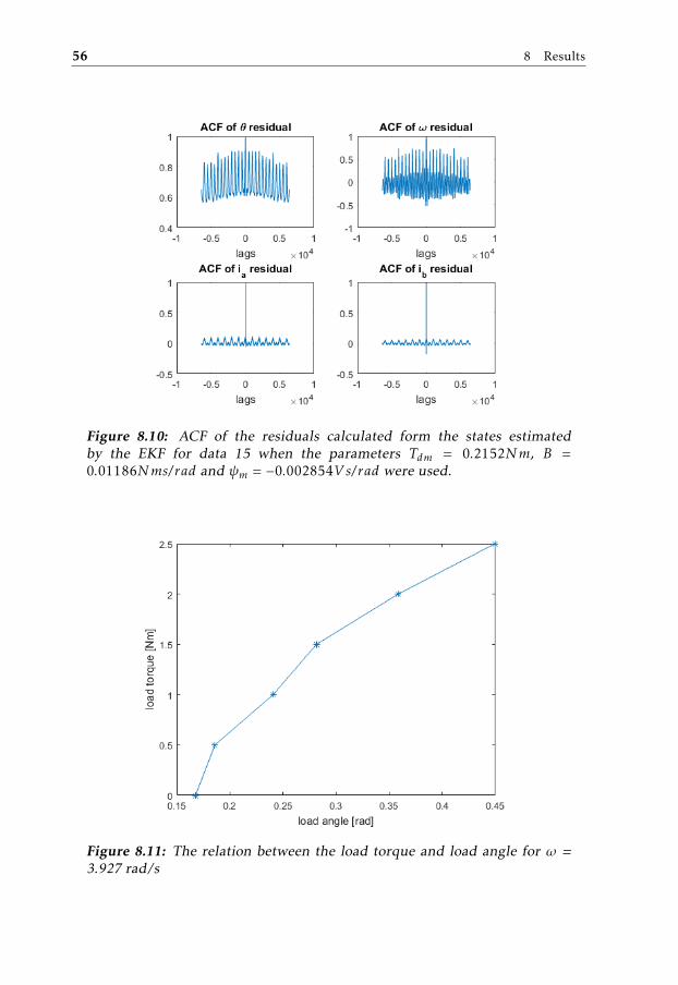
as low power as possible. However if the current is too low it is possible thatthe motor will loose steps. If step loss occurs it is possible that the estimates ofthe rotor angle will be incorrect. The step loss also causes unwanted noise andvibrations. To be able to gain information about the load and also to preventstep loss the load angle estimate is a good complement. In Chapter 3.2 it wasmentioned that the relation between the load angle and the load torque shouldbe sinusoidal. In Figure 8.11 it is possible to see the relations between the loadangle and load torque for rotor angular velocity 3.927 rad/s and at maximumrated current, 1.8 Amp. It can be seen in the figure that the appearance of thecurve is sinusoidal. At 3 Nm the motor will be stalled. In Figure 8.12 it can beseen how the load angle can vary when the rotor is completely stalled for onesecond. The fact that the rotor is stalled at 3 Nm is due to the holding torque,which is 3 Nm, see Table 4.2.
8.3 Evaluation of load angle estimations 53
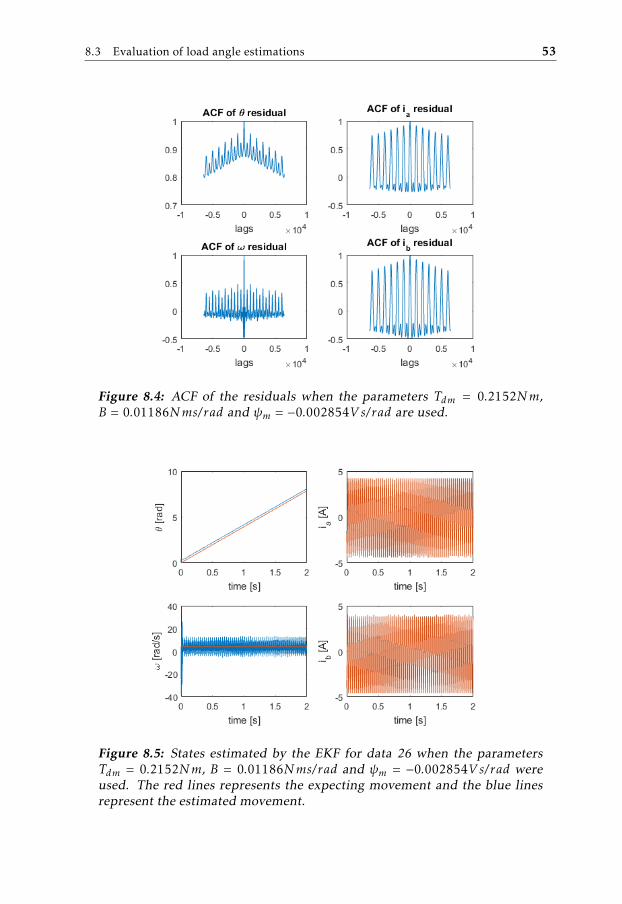
Figure 8.4: ACF of the residuals when the parameters Tdm = 0.2152Nm,B = 0.01186Nms/rad and ψm = −0.002854V s/rad are used.
Figure 8.5: States estimated by the EKF for data 26 when the parametersTdm = 0.2152Nm, B = 0.01186Nms/rad and ψm = −0.002854V s/rad wereused. The red lines represents the expecting movement and the blue linesrepresent the estimated movement.
54 8 Results
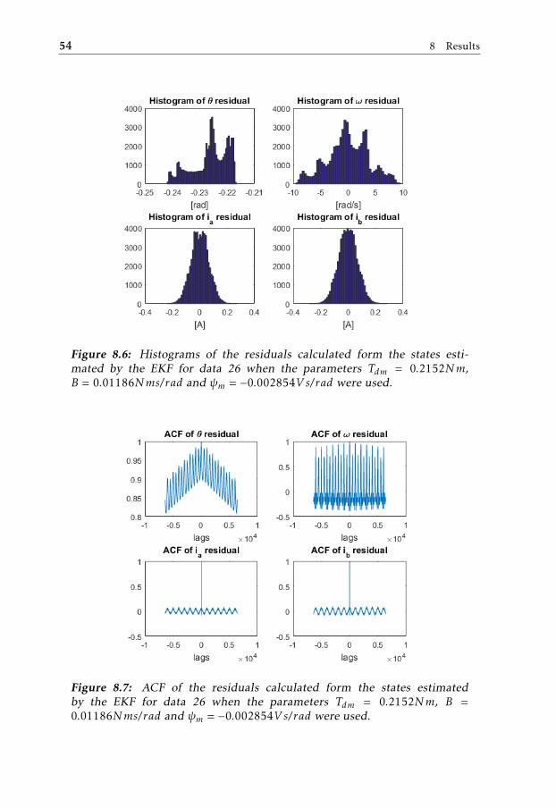
Figure 8.6: Histograms of the residuals calculated form the states esti-mated by the EKF for data 26 when the parameters Tdm = 0.2152Nm,B = 0.01186Nms/rad and ψm = −0.002854V s/rad were used.
Figure 8.7: ACF of the residuals calculated form the states estimatedby the EKF for data 26 when the parameters Tdm = 0.2152Nm, B =0.01186Nms/rad and ψm = −0.002854V s/rad were used.
8.3 Evaluation of load angle estimations 55
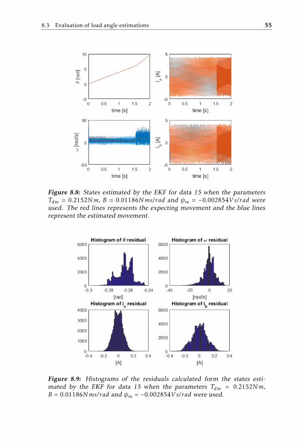
Figure 8.8: States estimated by the EKF for data 15 when the parametersTdm = 0.2152Nm, B = 0.01186Nms/rad and ψm = −0.002854V s/rad wereused. The red lines represents the expecting movement and the blue linesrepresent the estimated movement.
Figure 8.9: Histograms of the residuals calculated form the states esti-mated by the EKF for data 15 when the parameters Tdm = 0.2152Nm,B = 0.01186Nms/rad and ψm = −0.002854V s/rad were used.
56 8 Results
Figure 8.10: ACF of the residuals calculated form the states estimatedby the EKF for data 15 when the parameters Tdm = 0.2152Nm, B =0.01186Nms/rad and ψm = −0.002854V s/rad were used.
Figure 8.11: The relation between the load torque and load angle for ω =3.927 rad/s
8.3 Evaluation of load angle estimations 57
Figure 8.12: The appearance of the load angle when the motor is completelystalled.

9Discussion
In this chapter the results presented in Chapter 8 will be discussed. First a dis-cussion of the parameter determination will be done and it will be follow with adiscussion about the model. After that, the EKF and load angle estimate will bediscussed. Finally the chapter will present how the results from this thesis canbe used in the future.
9.1 Results
In this section the results presented in Chapter 8 will be discussed. First themodeling and parameter estimation will be discussed and after that follows adiscussion about the EKF and load angle estimation.
9.1.1 Motor model and parameters
The parameter estimation was not straight forward. Different methods, such aslinear regression for one parameter at a time, multiple linear regression for allparameters and EFK have been used, and all of them gave different parametersets. Residual analysis was used to determine which parameter set gave bestresult. Due to the lack of a positioning sensor, only theoretical values for theangle θ and angular velocity ω, could be compared with the estimated results.The precalculated values for the angular velocity ω was a constant value. Thisis true for the real system in a way that at least the mean of the actual velocityhas that value. Apart from this mean value it was impossible to know if thevariations in the estimated velocities were in accordance with the system. Thismade the parameter determination difficult since several parameters gave similarresults, and a positioning sensor had been helpful.
59
60 9 Discussion
One observation of the results is that the estimations of the rotor angle oftengives small constant biases. One explanation for this could be that the datasetsare collected when the motor is rotating at a constant velocity and then when thedataset is used in a simulation the model starts at velocity zero. It is a possibilitythat there is an internal inertia in the model to overcome before the modelledmotor can rotate as expected and this may create the biases seen in the results.
The model used in this thesis is a model based on basic electrical and mechan-ical equations. All system properties are not covered with the chosen model. Oneexample is that the electrical equations neglects the position and current depen-dence of the magnetic flux linkage and inductance. It is possible that the resultswould have been closer to the reference system if this dependence would havebeen added in the model. However, this would have increased the complexityand made all calculations more time consuming. A too complex model couldalso make estimations worse. In this thesis, focus was on creating a model toan estimator, which in the future should be possible to implement in a robot.Therefore the less complex model was preferable. Also the fact that authors in[2], [14] and [15] presented good result with the basic model made it natural toimplement that model.
9.1.2 EKF and load angle
The results from the EKF estimations showed good results. This provides thatthe model was a good choice. In the estimated velocity it is possible to see a noisyvariation. As mentioned earlier this variation could be explained by the motordesign. Because the motor takes steps by exiting its motor phases, the motionwill not be completely smooth. However, without a positioning sensor it is notpossible to say exactly how realistic these shown variations are, just that it islikely that some variations will exist.
The result of the load angle estimate seems promising. The relation betweenthe load torque and load angle shows the sinusoidal appearance as expected.However it was also expected that the load angle would be zero when the loadtorque was zero. As seen in the results the load angle is around 0.17 when theload torque is zero. The reason for this could be that the internal rotor torque,such as the detent torque or the torque produced due to friction, also affects theload angle.
When the motor is completely stalled the load angle varies rapidly. This isreasonable since a stall makes the rotor stop in one position fixing the back EMFvector. Meanwhile the current vector rotates with the excitation changes in thephases and therefore the load angle will change.
All implementation and calculations done in this master thesis are performedwith collected data with a very high sample time, almost 30 kHz. In a futureimplementation it is not possible to sample data this fast. The reason for why thedata were collected with this sample rate were because the phase voltage changedvery rapidly and when designing the model it was of interest to capture all modelproperties.
9.2 Future work 61
9.2 Future work
Since the EKF and the load angle has shown promising result it would be veryinteresting to take the evaluation of the hybrid stepper motor to the next level.This chapter will present suggestions for future work that can be done in thearea.
The first thing to investigate is how the estimated data will change if the sam-ple frequency changes. To sample the phase current at a lower rate should not bea problem. However problems could occur when it comes to the rapidly changingphase voltage.
9.2.1 Parameter determination
As mentioned in the previous discussion it was hard to distinguish differentdatasets from each other. In the report the prediction error is studied togetherwith residual analysis. Another method to distinguish datasets with similar bi-ases is to look at the root mean square, RMS, which is a measure of the variation.The RMS may give other datasets with better performance.
For determining the friction constant B, an assumption was made that thevelocity decreases linearly to zero. Further it was discussed that this assumptionmay be incorrect and therefore an approach where the velocity were assumedto decrease exponential were tested. In the report a conclusion were made thatthere were to many unknown signals to be able to determine B. However, whenthe rotor rotates it creates an induced voltage which affects the phase voltage ofthe system. When the power of the system is cut the measured phase voltage isassumed to be the induced voltage. Because of this, an assumption could madethat the relation between the rotor angular velocity and the phase voltage is
ω ∝ V (9.1)
Equation (6.3) can therefore be rewritten as
V = V (0) exp(−BJt)
(9.2)
To determine B linear regression can be used where
Y = ln
(VV (0)
)(9.3)
and
X =tJ
(9.4)
By using a dataset of the phase voltage when the power is cut and the motor decel-erates it is possible to determine B. Maybe this method can be used to determinea better data set.
62 9 Discussion
9.2.2 Extended Kalman Filter
In the EKF today, the load torque is seen as an unknown disturbance. Howeverit could be of interest to estimate the load torque as well. To make this possible amodel of the load torque needs to be developed. Since the robot shall be able tooperate in very varying areas it could be difficult to create a model that covers allvariations. However authors in [14] states that even a simple model of the loadtorque can provide good estimates and the area would therefore be interesting toinvestigate.
9.2.3 Load angle
To determine the load angle a test bench for breaking the motor was used. Withthis equipment it was possible to increase the load torque and observe how theload angle changed. The information given from the load angel can be used tocontrol the applied current when the robot reaches an uphill or an obstacle. Tobe able to do an accurate current control it is also important to know how theload angle is affected when the robot reaches a downhill, and the load torque isnegative. To be able to investigate this an experiment can be made where themotor is pushed by another motor.
The load angle varies when there is a change in load torque or current. This isbecause a change in the current changes the produced torque. Also the velocitycan affect the load angle since a higher velocity reduces the produced torque.I order to utilize all information in the load angle it could be of high interestto investigate how the relationship between the load angle and the load torquechanges for different velocities and currents.
When the behaviour of the load angle is known it can be used for stall de-tection. The most simple way is to implement a threshold function as adaptswith the rotor speed and the applied load torque. This implementation can forexample be used to detect collisions.
10Conclusions
This master thesis has investigated the possibilities to replace a BLDC-motor anda gearbox with a hybrid stepper motor. The main goal was to develop a possibleestimator for estimating information about the motor that could be used in afuture speed and torque control algorithm.
This thesis work has been treating modelling and estimations of a hybrid step-per motor. For modelling fundamental electrical and mechanical equations wereused. Decisions were made that a model based on these equations will be ableto describe the needed system behaviour and therefore an extended model werenot developed. It is advantageous to use the basic model in a future implemen-tation because it will be less time consuming as a more complex model. A majorproblem with the modelling has been the lack of a positioning sensor. This madeit difficult do determine which parameter set that best described the real system.There is a possibility that other parameter sets can describe the system better.
For estimations of the rotor angle and angular velocity an EKF has been tested.The EKF is used because it allows the model to be nonlinear. When tuned cor-rectly the EKF gives good results of the estimations. Also here a problem oc-curred due to the lack of a positioning sensor because the data to compare withwas not as accurate as might have been desirable.
As a complement to the EKF estimates the load angle was investigated. Therelation between the load angle and the load torque would, according to authorsin [7], be sinusoidal and that was also the result of the investigation in this thesis.For implementing the load angle estimation the sliding discrete fourier transformwas used. This variant of the fourier transform makes it possible to update theload angle estimate in a more efficient way.
The goal of this master thesis was to investigate the possibility to develop asensorless estimator to a Hybrid Stepper Motor. This to examine if it is possibleto replace a BLDC-motor together with a gearbox with a Hybrid Stepper motor.
63
64 10 Conclusions
It was shown that an EKF which estimates the rotor angle and rotor angular ve-locity, together with a load angle estimate should be able to give enough feedbackto a controller. The results of this thesis can be used as a basis for further investi-gations on the Hybrid Stepper motor. This to decide whether a stepper motor isa good alternative for propulsion of autonomous lawn mowing robots.
Bibliography
[1] P. P. Acarnley. Stepping motors : a guide to theory and practice, fourthedition. [Elektronisk resurs]. IEE control engineering series: 63. London: Institution of Electrical Engineers, c2002. ISBN 0852960298. Cited onpages 7 and 8.
[2] M. Bendjedia, Y. Ait-Amirat, B. Walther, and A. Berthon. Position controlof a sensorless stepper motor. IEEE Transactions on Power Electronics, 27(2):578–587, Feb 2012. ISSN 0885-8993. doi: 10.1109/TPEL.2011.2161774.Cited on pages 5, 6, and 60.
[3] S. Bolognani, L. Tubiana, and M. Zigliotto. Extended kalman filter tuningin sensorless pmsm drives. IEEE Transactions on Industry Applications, 39(6):1741–1747, Nov 2003. ISSN 0093-9994. doi: 10.1109/TIA.2003.818991.Cited on page 37.
[4] M. Butcher, A. Masi, R. Picatoste, and A. Giustiniani. Hybrid stepper motorelectrical model extensions for use in intelligent drives. IEEE Transactionson Industrial Electronics, 61(2):917–929, Feb 2014. ISSN 0278-0046. doi:10.1109/TIE.2013.2254097. Cited on pages 5 and 6.
[5] S. Derammelaere, L. Carlier, B. Vervisch, C. Debruyne, K. Stockman, L. Van-develde, P. Cox, and G. Van den Abeele. The opportunities of two-phase hy-brid stepping motor back emf sampling. In 2011 IEEE Energy ConversionCongress and Exposition, Technical University College of West-Flanders, Ko-rtrijk, Belgium, . Cited on page 6.
[6] S. Derammelaere, C. Debruyne, F. D. Belie, K. Stockman, and L. Vandevelde.Load angle estimation for two-phase hybrid stepping motors. IET ElectricPower Applications, 8(7):257–266, August 2014. ISSN 1751-8660. doi: 10.1049/iet-epa.2013.0333. Cited on pages 6 and 11.
[7] Stijn Derammelaere, Colin Debruyne, Frederik De Belie, Kurt Stockman,and Lieven Vandevelde. Load angle estimation for two-phase hybrid step-ping motors. IET Electric Power Applications, 8(7):257 – 266, . ISSN17518660. doi: 10.1049/iet-epa.2013.0333. Cited on pages 5, 6, 10, 11,46, 47, and 63.
65
66 Bibliography
[8] Mille Millnert Fredrik Gustafsson, Lennart Ljung. Signal Processing. Stu-dentlitteratur, 1:3 edition, 2010. ISBN 978-91-44-05835-1. Cited on page13.
[9] Fredrik Gustafsson. Statistical Sensor Fusion. Studentlitteratur, 2:1 edition,2012. ISBN 978-91-44-07732-1. Cited on page 13.
[10] T. A. Khan, T. A. Taj, and I. Ijaz. Hybrid stepper motor and its control-ling techniques a survey. In Electrical and Electronic Engineering Con-ference (ElConRusNW), Proceedings of the 2014 IEEE NW Russia YoungResearchers in, pages 79–83, Feb 2014. doi: 10.1109/ElConRusNW.2014.6839207. Cited on page 5.
[11] Torkel Glad Lennart Ljung. Modellbygge och simulering. Studentlitteratur,2:5 edition, 2004. ISBN 978-91-44-02443-1. Cited on page 12.
[12] Bertil Westergren Lennart Råde. Mathematics Handbook, for Scinece andEngineering. Studentlitteratur, 5:12 edition, 2004. ISBN 978-91-44-03109-5. Cited on page 13.
[13] Allegro MicroSystems LLC. Dual Full-Bridge MOSFET Driver with Mi-crostepping Translator. Cited on page 15.
[14] J. Persson and Y. Perriard. An optimized extended kalman filter algorithmfor hybrid stepper motors. In Industrial Electronics Society, 2003. IECON’03. The 29th Annual Conference of the IEEE, volume 1, pages 297–300vol.1, Nov 2003. doi: 10.1109/IECON.2003.1279995. Cited on pages 5, 6,60, and 62.
[15] D. Samokhvalov, S. Stoliarov, and A. Kekkonen. The hybrid stepper motormodeling in simulink. In Young Researchers in Electrical and ElectronicEngineering Conference (EIConRusNW), 2015 IEEE NW Russia, pages 282–285, Feb 2015. doi: 10.1109/EIConRusNW.2015.7102280. Cited on pages 5,6, 23, 25, and 60.
[16] Stephen D. Umans. Fitzgerald & Kingsley’s Electric Machinery. McGraw-Hill Education, seventh international edition edition, 2014. ISBN 978-1-259-25466-6. Cited on pages 5 and 7.
[17] Sanford Weisberg. Applied linear regression. [Elektronisk resurs]. Wiley Se-ries in Probability and Statistics. Hoboken, New Jersey : Wiley, 2014., 2014.ISBN 9781118386088. Cited on page 12.