sensors-09-07753

7/31/2019 sensors-09-07753

http://slidepdf.com/reader/full/sensors-09-07753 1/18

Sensors 2009, 9, 7753-7770; doi:10.3390/s91007753

sensorsISSN 1424-8220

www.mdpi.com/journal/sensors

Article

Defect Detection in Arc-Welding Processes by Means of the

Line-to-Continuum Method and Feature Selection

P. Beatriz Garcia-Allende *, Jesus Mirapeix, Olga M. Conde, Adolfo Cobo and

Jose M. Lopez-Higuera

Photonics Engineering Group, University of Cantabria, Avda. de los Castros S/N, 39005 Santander,

Spain; E-Mails: [email protected] (J.M.); [email protected] (O.M.C.);

[email protected] (A.C.); [email protected] (J.M.L.-H.)

* Author to whom correspondence should be addressed; E-Mail: [email protected];

Tel.: +34-942-200877; Fax: +34-942-200877.

Received: 8 July 2009; in revised form: 28 August 2009 / Accepted: 24 September 2009 /

Published: 29 September 2009

Abstract: Plasma optical spectroscopy is widely employed in on-line welding diagnostics.

The determination of the plasma electron temperature, which is typically selected as the

output monitoring parameter, implies the identification of the atomic emission lines. As a

consequence, additional processing stages are required with a direct impact on the real time

performance of the technique. The line-to-continuum method is a feasible alternative

spectroscopic approach and it is particularly interesting in terms of its computational

efficiency. However, the monitoring signal highly depends on the chosen emission line. In

this paper, a feature selection methodology is proposed to solve the uncertainty regarding

the selection of the optimum spectral band, which allows the employment of the line-to-

continuum method for on-line welding diagnostics. Field test results have been conducted

to demonstrate the feasibility of the solution.

Keywords: arc-welding; plasma spectroscopy; feature selection; on-line monitoring

OPEN ACCESS

7/31/2019 sensors-09-07753


Sensors 2009, 9 7754

1. Introduction

The fields where welding processes are key factors in the production stages cover a wide range of

different applications: manufacturing of pipes for various sectors, engines for aeronautics, automobiles

or heavy components for nuclear power stations are some relevant examples in this regard. The lack of a complete comprehension of the physical phenomena occurring during the welding process, and the

demanding quality standards to be found in this framework, have forced scientists to carry out an

intense research effort in both welding physics and procedures devoted to cope with quality issues.

Some of these studies have been focused on the development of theoretical models for both arc and

laser welding [1-3], including numerical analysis approaches [4]. These efforts help to understand the

process and, therefore, to determine the precise input parameter ranges that will provide seams free

of flaws.

However, in practice welding coupons employed for parameter adjustment, and both destructive

and non-destructive trials [5] have to be used to ensure that the performed seams satisfy the established

quality standards. This obviously implies a significant cost in terms of productivity, as a lot of time is

spent before and after the welding process itself, and, therefore, some of the seams have to be

reworked and evaluated again.

This scenario has led to an intense research effort aimed at developing efficient and reliable on-line

welding quality monitoring systems. They should be able to detect in real-time the occurrence of

possible defects and, as an added value, to control the welding setup to try to avoid these defects or

drifts from the standard operation conditions. Several techniques have been proposed, from electrical

and capacitive sensors [6,7], to monitoring based on the analysis of the acoustic signal generated

during the process [8,9] or solutions based on machine vision [10,11]. Among these alternatives, the

optical analysis of the welding plasma radiation has proved to be a feasible and promising option.

Initial proposals were based on the use of photodiodes and the analysis of emissions in the ultraviolet,

visible and infrared regions [12], determining for example the full-penetration condition in laser

welding [13].

A more sophisticated approach has been proposed by considering plasma optical spectroscopy,

where emission lines appearing in the plasma spectra are analyzed to provide a plasma electron

temperature T e profile that shows a direct correlation to weld defects [14,15]. In the last years, several

publications have dealt with refinements of this technique, allowing automatic defect detection [16]and reducing the overall computational cost of the system [17]. More recently, new strategies have

been proposed to extract more information from the plasma spectra, like the correlation analysis

proposed by Sibillano et al. [18], or proposals based on the use of optimization algorithms to generate

synthetic spectra [19]. Within the same framework, new spectroscopic parameters are also being

studied in an attempt to improve the monitoring system efficiency [20].

One of the key issues when using plasma spectroscopy lies in the correct selection of the emission

lines chosen to calculate the output monitoring parameter. On the one hand, and depending on the

selected instrumentation, there can be ambiguities on the emission line identification, what can end in

unexpected results. On the other hand, and especially when defect classification is required, i.e., to beable to distinguish among different types of defects, it would be highly interesting to know which

emission lines allow a better discrimination for classification purposes.

7/31/2019 sensors-09-07753


Sensors 2009, 9 7755

We have conducted some previous studies by using PCA (Principal Component Analysis) and

SFFS (Sequential Forward Floating Selection) to feed an Artificial Neural Network [21,22]. The use of

SFFS allows to gain knowledge about the best spectral bands selected. This will be used in this paper

to propose a scheme based on both the SFFS algorithm and the line-to-continuum method [23] to

generate the required output monitoring profiles. The line-to-continuum method implies the use of

only a single emission line that, in addition, does not need to be identified, i.e., associated with its

chemical species.

2. Plasma Optical Spectroscopy for Welding Diagnostics

The plasma electron temperature has been widely used as the output monitoring parameter for

welding diagnostics, given the known correlation between its profiles and the appearance of defects in

the seams. There are basically two approaches that are employed in the literature: a precise estimation

of T e can be obtained with the Boltzmann-plot method [23]:

e

m

mmn

mnmn

kT

E

Z

hcN

g A

I −⎟

⎠

⎞⎜⎝

⎛ =⎟⎟

⎠

⎞⎜⎜⎝

⎛ lnln

λ (1)

where several emission lines from the same species are involved in the calculations. In the previous

equation I mn is the relative intensity of the chosen emission line, m and n the upper and lower states,

respectively, λmn the central wavelength associated with the line, Amn the transition probability, g m the

statistical weight, h the Planck’s constant, c the light velocity, N the population density of the state m,

Z the partition function, E m the upper level energy and k the Boltzmann constant. T e can be obtained if

the left-hand side of Equation (1) is represented versus E m, given that the slope of the resulting line is

inversely proportional to the temperature.

On the other hand, and due to considerations regarding the computational performance of the

monitoring system, which determines its spatial resolution, a simplification of the Boltzmann-plot

method, where only two emission lines are involved, is typically used:

⎥⎦

⎤⎢⎣

⎡

−=

)2()1()1()2()2(

)1()2()2()1()1(ln

)1()2(

λ

λ

mm

mm

mme

g A I E

g A I E k

E E T

(2)

This equation was proposed by Marotta [24] for arc-welding processes. The commented techniques

can be equally applied to both arc and laser processes, although for the latter the energies of the upper

level disappear from the logarithm in the denominator.

Although different approaches can be taken into account, a possible processing scheme designed to

provide the required T e estimation from the acquired welding plasma spectra is presented in Figure 1.

The identification of the emission lines is compulsory to obtain T e. As shown in Figure 1, this

requires three additional processing stages (peak detection and line modeling and identification) and it

has, as a consequence, a direct implication in the real-time performance of the overall approach. An

alternative solution is to perform a previous spectral band selection stage with a data set consisting of

spectra from the same welding process under different conditions. Afterwards those lines can be used

without involving the identification in the processing scheme.

7/31/2019 sensors-09-07753


Sensors 2009, 9 7756

Figure 1. Comparison of the processing schemes associated with the traditional approach

and the proposed solution based on SFFS and the line-to-continuum method.

This could be applied for scenarios where the same materials and welding conditions are used, but it

limits the flexibility of the analysis strategy. On the other hand, as previously commented, there is a

lack of knowledge on the selection of the optimal emission lines for welding diagnostics. Some studies

have been carried out comparing the response of different elements and species, but we believe that byspecifically searching for the most discriminant spectral bands the overall performance of the

monitoring system should be improved.

Within this framework, the use of the line-to-continuum method to generate the output monitoring

profiles seems to be a good solution, given that it does not require the identification of the chosen

emission line. However, it could be performed to avoid problems related to the effect of unresolved

lines. This method was originally intended to estimate T e by means of the following expression [25]:

( )λ

λ

ξ λ

ε

Δ⎟⎟

⎠

⎞⎜⎜

⎝

⎛ −×= −

e

mi

ei

mmn

c

l

kT

E E

T Z

g A

I exp

1100052.2 5 (3)

where εl is the line intensity integrated over the line profile, I c the intensity of the adjacent background

radiation (non-integrated), Z i is the ion partition function, ζ the free-bound continuum correction, E i the

ionization potential and Δλ the wavelength bandwidth. It is worth mentioning that an iterative method

has to be employed to determine T e via Equation (3). However, in the proposed method we only use

the εl / I c ratio as the monitoring parameter. In a previous paper, this approach was initially explored in

comparison to an alternative method based on the estimation of the wavelength associated with the

maximum intensity of the continuum radiation [20]. In this case we concluded that the line-to-

continuum method could not be reliably used given the uncertainty regarding the selection of the

spectral band for the subsequent analysis. In this paper the use of the SFFS algorithm will help to deal

with this issue.

7/31/2019 sensors-09-07753


Sensors 2009, 9 7757

3. Sequential Floating forward Selection of Spectral Bands

The Sequential Floating Forward Selection (SFFS) algorithm [26] is widely applied to reduce the

dimensionality, i.e., the number of features or wavelengths, of spectral data prior to their

interpretation [27,28]. The spectral band selection criterion is based on the capability of the distinctfeatures to separate the different classes to be discriminated afterwards. The greater the separability

between the classes that a wavelength provides, the better the wavelength is for classification purposes.

Therefore, a similar approach could be followed to solve the uncertainty encountered in the selection

of the optimum band within the plasma spectra for on-line welding quality monitoring by means of the

line-to-continuum method described above [20]. The aim of SFFS is to select M spectral bands that

best discriminate among correct welds and flaws, out of the total number of initial bands N , so M << N .

In this way the line-to-continuum profiles obtained later on for these M bands will be optimized for

defect detection. It is worth highlighting here that SFFS has already been used in some previous works

by our group [22]. However, the focus was, on the contrary, to provide a set of spectral bands to feed

an Artificial Neural Network (ANN) for flaw discrimination as an alternative to the widely known

feature extraction techniques [21].

As mentioned before, the selection criterion for band selection is an objective function based on a

measurement of the separability of the classes. Specifically, it is estimated in terms of the

Bhattacharyya distance as in [22]:

( ) [ ] ( )

⎟⎟⎟⎟⎟⎟

⎠

⎞

⎜⎜⎜⎜⎜⎜

⎝

⎛

⎟ ⎠ ⎞

⎜⎝ ⎛

∑⋅∑

∑+∑+−∑+∑−=

2

1

212

21log

2

1

1221124

1μ μ μ μ T

B J

(4)

where μi is the mean of the i class; ∑i its covariance matrix and |∑i| stands for the determinant of matrix

∑i There are only two classes to be distinguished here: correct seams and defects. Therefore, the

overall separability among the classes to be discriminated is straightly given by (4).

Figure 2. Spectral curves of: (a) several correct seams. (b) distinct flaws.

Wavelength (nm)

I n t e n s i t y ( a . u . )

I n t e n s i t y ( a . u . )

Wavelength (nm)

(a) (b)

In Figure 2 several spectral curves of correct welds (a) and defects (b) are presented. As shown,

some ranges of the spectra exhibit similar characteristics and, as a consequence, they are useless for

7/31/2019 sensors-09-07753


Sensors 2009, 9 7758

defect detection purposes. The elimination of these ranges is compulsory prior to the application of

SFFS. This procedure is named data decorrelation since only one spectral band, the one that

maximizes the Bhatacharya distance, is selected within each redundant block. Each redundant block is

obtained as a wavelength range where spectral bands have a high correlation coefficient, nearly 1.

Figure 3. Block diagram of the spectral band selection and sorting procedure.

Data decorrelation SFFS

383.6

416.3

447.9

478.4

507.8

383.6 416.3 447.9 478.4 507.80

1

0.8

0.6

0.4

0.2

Wavelength (nm)

W a v e l e n g t h ( n m )

Correlation coefficient matrix between all thespectral bands

M uncorrelated

band blocks

M << 1180

N = 1180

Blocks of correlated spectral bands applying a

0.99 threshold

383.6

416.3

447.9

478.4

507.8

383.6 416.3 447.9 478.4 507.8Wavelength (nm)

W a v e l e n g t h ( n m )

N initial

bands

M spectral bands

sorted according

their

discrimination

capability

M uncorrelated

spectral bands

SFFS is named “ forward ” because it begins with an empty selected feature subset. It initially selects

from the uncorrelated subset of spectral bands the most discriminant one according to the

Bhattacharyya distance. Then it carries on sequentially adding the second most discriminant

wavelength and so on. Therefore, in each iteration a new spectral band is added. However, if the

iteration number is greater than 1, some of the previously added features can be removed if the

separability of the classes enhances. Then, after every forward step (addition of a new spectral band) a

number of backward steps (removal of several spectral bands) are applied as long as the resultingsubsets are better than the previously evaluated ones according to the Bhatacharrya distance, and for

that reason the selection procedure is also named “ floating ”. This procedure continues until some

7/31/2019 sensors-09-07753


7/31/2019 sensors-09-07753


Sensors 2009, 9 7760

line. Figure 4 shows the discrepancies to be found in the line-to-continuum profiles depending on the

spectral band selected. In these profiles I L stands for the relative intensity of the chosen spectral band

and I C for the corresponding background radiation.

Figure 4. Detection of weld flaws by means of line-to-continuum method: a) and b) bead-on-plate seams with defects; c) and d) output profiles with spectral band 518.41 nm; e) and

f) output profiles with spectral band 375.03 nm; g) and h) output profiles with spectral

band 481.08 nm.

Figure 4c,d presents the results obtained with spectral band 518.41 nm, Figure 4e,f with 375.03 nm

and Figure 4g,h with 481.08 nm. The latter offers the best results in terms of defect discrimination,given that the three flaws located at x ≈ 6 cm for seam nº 1 [Figure 4a], and at x ≈ 5 and 7 cm for seam

nº 2 (Figure 4b) are associated with rapid perturbations on the profiles. On the contrary, Figure 4c,d

7/31/2019 sensors-09-07753


Sensors 2009, 9 7761

does not show any correlation with these defects, indicating that the selected spectral band is not

suitable in this case. By using the spectral band located at 375.03 nm the identification of the defects is

again feasible, but the signal-to-noise ratio is clearly poorer in this case. It is worth mentioning that the

dip at the beginning of Figure 4g is due to the use of a lower welding current at the beginning of the

process. As expected, a lower plasma electron temperature is associated with a lower welding current,

given that the line-to-continuum profile is directly related to this parameter as suggested by

Equation (3). The slope of Figure 4h was caused by a non-constant distance between the electrode tip

and the plate provoked by the deformation of the plate by heat during previous seams. Again, the slope

is associated with T e, being the temperature higher as the distance between the electrode tip and the

plate becomes smaller. These two situations can be also considered as defective, although the analysis

via SFFS has been performed considering only the sections highlighted in Figure 4a,b as weld defects.

An example of automatic weld defect detection has been included in Figure 4g, using the approach

proposed by Ancona et al. in [16]. In this case the reference signal has been generated considering the

seam section between x ≈ 3.5 and x ≈ 5.5 cm as correct. The corresponding thresholds have been

plotted by determining both the I L /I C mean and standard deviation values, and chosing α = 10 [16]. It

can be observed that not only the defect at x ≈ 6 cm, but also the lack of penetration at the beginning of

the seam would be identified as defective, as the monitoring signal exceeds the calculated thresholds.

The same analysis has been conducted in Figure 4h, where again the signal associated with the defects

under analysis and the initial section of the seam exceeds the thresholds.

The results related to spectral bands 375.03 and 518.41 nm are worse than expected taking into

account that their selection by the SFFS algorithm is performed earlier than the selection of the 481.08

nm spectral band. An initial analysis indicates that a possible explanation lies in the suppression of bands correlated to these ones that would offer better correlation to the quality of the seams. This

occurs for example between spectral bands located at 375.03 and 446.07 nm. The latter gives rise to

profiles similar to the ones depicted in Figure 4g,h, but this band is correlated to the former and,

consequently, suppressed by the SFFS algorithm.

The plasma spectra for both experimental tests and spectral bands have been represented in Figure 5.

It can be appreciated how the band chosen by SFFS does not belong to an emission line, while in

446.07 nm a significant peak is to be found.

A feasible explanation for the uncertainty in the SFFS sorting criterion of the spectral bands is

based on its assumptions about the probability distribution functions of the data. The employment of

the SFFS algorithm implies a Gaussian or normal distribution of the classes. Correct welding could fit

with this assumption but this is not necessarily the case of the defect class taking into the account the

complexity of the physical phenomena occurring during the processes. An easy way to estimate

whether the class distributions are Gaussian or not is by evaluating its third and fourth order statistics

moments, namely skewness and kurtosis [29].

7/31/2019 sensors-09-07753


Sensors 2009, 9 7762

Figure 5. Comparison of spectra associated with correct and defective seams: a) and b)

spectral band 375.03 for seams nº 1 and 2; c) and d) spectral band 446.07 for seams nº 1

and 2.

Skewness is a measure of the asymmetry of the data around the class mean. Therefore the skewness

of the normal distribution (as in any other perfectly symmetric distribution) is zero. Kurtosis is a

measure of how outlier-prone a class distribution is and the kurtosis of the normal distribution is 3.

Skewness and kurtosis values per class and wavelength are displayed in Figure 6a,b, respectively,

while Figure 6c-f exhibits their corresponding histograms. Neither the skewness histogram pertaining

to the correct welding class nor the one pertaining to defects are centered around zero, which allows us

to conclude that none of the classes have a normal distribution. In spite of this fact, SFFS provides the

selection of some spectral bands that allow defect detection such as the one in 481.08 nm and, as a

consequence, a two step methodology is proposed. First the SFFS algorithm is applied and the

line-to-continuum profiles are obtained for the selected wavelengths. Then the signal-to-noise ratio of these profiles is evaluated and the one with the highest value is selected as the monitoring signal.

7/31/2019 sensors-09-07753


Sensors 2009, 9 7763

Figure 6. Modelling of the data distribution function of the classes: a) and b) skewness and

kurtosis values per class and wavelength; c) histogram of skewness values of correct

weldings d) histogram of skewness values of defects; e) and f) idem for kurtosis values.

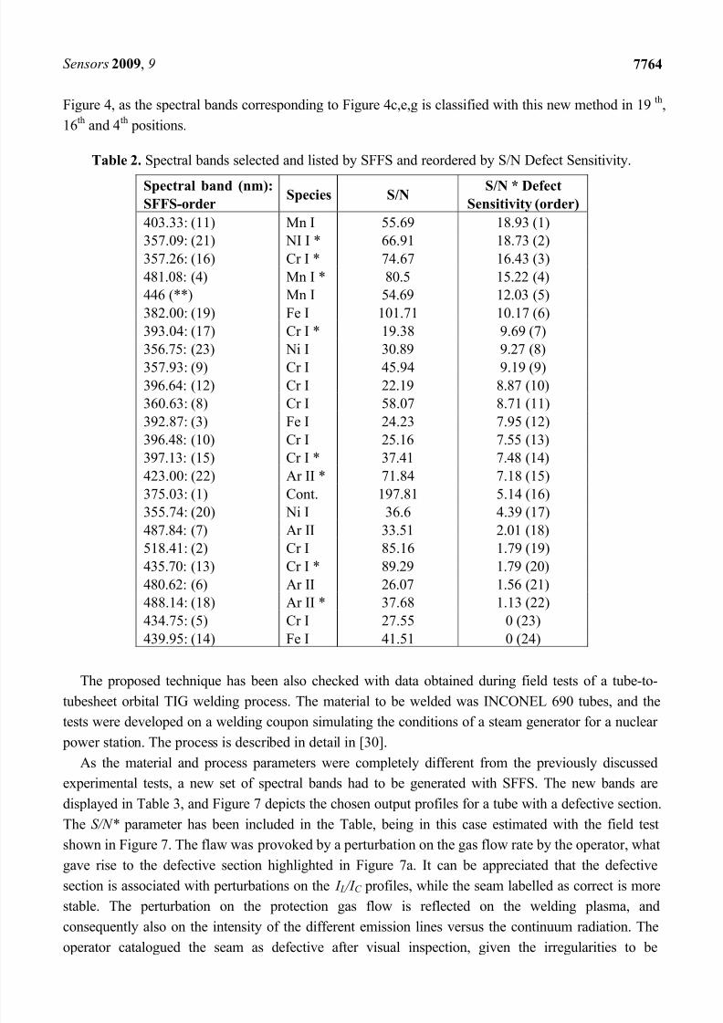
The reordering of the spectral bands in terms of the S/N* (Defect Sensitivity) parameter is presented

in Table 2. A detailed study of the resulting line-to-continuum profiles was conducted to elucidate a

suitable method to quantify their sensitivity to detect the weld flaws. This S/N* is calculated as follows:

first, the signal-to-noise ratio over a section free of defects is estimated (S/N in Table 2), being in this

case the seam segment between welding times 3 and 5 s for seam nº 1. Afterwards, the defect detection

sensitivity is considered as the difference between the I L /I C value at the defect (x ≈ 6 s) and x = 5.5,

where the signal indicates a correct seam. Finally, this two values are multiplied to generate the S/N* parameter. This new ordering of the spectral bands is in good agreement with the results shown in

7/31/2019 sensors-09-07753


Sensors 2009, 9 7764

Figure 4, as the spectral bands corresponding to Figure 4c,e,g is classified with this new method in 19th

,

16th

and 4th

positions.

Table 2. Spectral bands selected and listed by SFFS and reordered by S/N Defect Sensitivity.

Spectral band (nm):

SFFS-orderSpecies S/N

S/N * Defect

Sensitivity (order)

403.33: (11) Mn I 55.69 18.93 (1)

357.09: (21) NI I * 66.91 18.73 (2)

357.26: (16) Cr I * 74.67 16.43 (3)

481.08: (4) Mn I * 80.5 15.22 (4)

446 (**) Mn I 54.69 12.03 (5)

382.00: (19) Fe I 101.71 10.17 (6)

393.04: (17) Cr I * 19.38 9.69 (7)

356.75: (23) Ni I 30.89 9.27 (8)

357.93: (9) Cr I 45.94 9.19 (9)

396.64: (12) Cr I 22.19 8.87 (10)

360.63: (8) Cr I 58.07 8.71 (11)

392.87: (3) Fe I 24.23 7.95 (12)

396.48: (10) Cr I 25.16 7.55 (13)

397.13: (15) Cr I * 37.41 7.48 (14)

423.00: (22) Ar II * 71.84 7.18 (15)

375.03: (1) Cont. 197.81 5.14 (16)

355.74: (20) Ni I 36.6 4.39 (17)

487.84: (7) Ar II 33.51 2.01 (18)518.41: (2) Cr I 85.16 1.79 (19)

435.70: (13) Cr I * 89.29 1.79 (20)

480.62: (6) Ar II 26.07 1.56 (21)

488.14: (18) Ar II * 37.68 1.13 (22)

434.75: (5) Cr I 27.55 0 (23)

439.95: (14) Fe I 41.51 0 (24)

The proposed technique has been also checked with data obtained during field tests of a tube-to-

tubesheet orbital TIG welding process. The material to be welded was INCONEL 690 tubes, and the

tests were developed on a welding coupon simulating the conditions of a steam generator for a nuclear

power station. The process is described in detail in [30].

As the material and process parameters were completely different from the previously discussed

experimental tests, a new set of spectral bands had to be generated with SFFS. The new bands are

displayed in Table 3, and Figure 7 depicts the chosen output profiles for a tube with a defective section.

The S/N* parameter has been included in the Table, being in this case estimated with the field test

shown in Figure 7. The flaw was provoked by a perturbation on the gas flow rate by the operator, what

gave rise to the defective section highlighted in Figure 7a. It can be appreciated that the defective

section is associated with perturbations on the I L /I C profiles, while the seam labelled as correct is more

stable. The perturbation on the protection gas flow is reflected on the welding plasma, and

consequently also on the intensity of the different emission lines versus the continuum radiation. The

operator catalogued the seam as defective after visual inspection, given the irregularities to be

7/31/2019 sensors-09-07753


Sensors 2009, 9 7765

observed on the surface, as well as the associated bead color. Further analyses by means of destructive

or non-destructive evaluation techniques could have helped to improve this classification, but in this

case visual inspection was considered to be adequate. According to the ISO 6520-1:1998 standard this

defect could be labelled as an irregular surface (excessive surface roughness). Four different spectral

bands have been considered in this case: 404.14, 422.84, 480.52 and 423.64 nm. It is precisely the

latter, associated with Fe I, the one which exhibits worst results in terms of sensitivity to defects, as all

the profiles have been represented with the same vertical scale. It is important highlighting that the

defective section could be identified, at least partially, in the four cases, but the profile in Figure 7c

offers the best sensitivity: in terms of S/N* the spectral bands are classified as 7th (404.14 nm), 2nd

(422.84 nm), 8th

(480.52 nm) and 10th

(423.64 nm). The I L /I C thresholds have been calculated again for

Figure 7c, using in this case α = 3.

Table 3. Spectral bands selected and listed by SFFS and related to species participating in

the plasma: field tests.

Spectral band (nm):

(SFFS-order)Species S/N S/N * (order)

516.79 (12) Fe I 29.1 41.03 (1)

422.84 (3) Ar II 16.1 24.30 (2)

415.95 (2) Ar I 20.96 20.54 (3)

402.83 (6) Mn I * 30.68 19.68 (4)

426.35 (5) Cr I * 28.42 15.92 (5)

407.39 (9) Cont. 42.69 14.94 (6)

404.14 (1) Mn I * 13.91 14.47 (7)480.52 (7) Ar II 20.24 14.37 (8)

443.54 (11) Fe I 28.57 14.00 (9)

423.64 (4) Fe I 26.1 11.48 (10)

478.28 (8) Mn I 26.28 11.30 (11)

432.28 (14) Cont. 36.9 7.38 (12)

427.30 (10) Cr I 52.77 3.69 (13)

520.05 (13) Cr I 19.1 1.53 (14)

A different defect is presented in Figure 8a, where a porosity (highlighted in red) was created due tothe application of a gel to the tube-to-tubesheet interface. It is interesting to note that, although only

the porosity appears as visible, the gel was applied trough the whole interface, what probably provoked

deviations from the standard quality requirements. This can be the explanation to the fast perturbations

that appear in the profiles of Figure 8b-e. Again, Figure 8c, where the I L /I C thresholds have been

plotted, offers the best identification of the porosity and the higher defect sensitivity. It is interesting to

note that in this case the classification provided by S/N* seems valid for the first three bands, but the

fourth (Figure 8e) exhibits a better response than Figure 8b, for example. This can be explained

because the S/N* analysis was performed with the field test associated with Figure 7. In this case the

generalization of these classifications to both seams would not be valid, and a separate study should be

conducted.

7/31/2019 sensors-09-07753


Sensors 2009, 9 7766

Figure 7. Field test tube with defective section: a) welded tube; b) profile for spectral band

404.14 nm; c) profile for spectral band 422.84 nm; d) profile for spectral band 480.52 nm;

e) profile for spectral band 423.64 nm.

7/31/2019 sensors-09-07753


Sensors 2009, 9 7767

Figure 8. Field test tube with porosity: a) welded tube; b) profile for spectral band 404.14 nm;

c) profile for spectral band 422.84 nm; d) profile for spectral band 480.52 nm; e) profile for

spectral band 423.64 nm.

5. Conclusions

A spectroscopic approach based on feature selection and the line-to-continuum method for on-line

detection of welding defects is proposed and experimentally validated in this paper. Compared with

the determination of the plasma electron temperature, the main advantage of the line-to-continuum

method is its computational efficiency, since it does not imply the identification of the atomic emissionlines. However, its defect detection capability highly depends on the chosen emission lines. Therefore,

an initial stage is required to determine those spectral bands from the welding plasma that best

7/31/2019 sensors-09-07753


Sensors 2009, 9 7768

discriminate among correct welding and the appearance of defects. In a previous work [22] the SFFS

algorithm was employed to reduce spectral dimensionality of data from an embedded fiber-sensor for

on-line welding diagnostics. Selection criterion of the spectral bands was based on the maximization of

the distance between the different flaws and correct welds. This same approach has been applied here

to get rid of the uncertainty regarding the selection of the optimum spectral bands. SFFS is firstly

utilized to identify the proper lines for defect detection. Then, the monitoring signal consists of the

line-to-continuum profiles of those lines. Experimental results show a strong correlation between the

appearance of flaws and abrupt changes in the monitoring signal.

The conducted studies, which include an extended set of defects with different target materials,

have demonstrated the suitability of the methodology for on-line analysis. However, they have also

brought up that some uncertainty still remains regarding the SFFS sorting criterion of the spectral

bands. As shown, it occurs that some of the spectral bands that are selected later on by SFFS have

proved more successful in defect-detection. This is due to the fact that the wavelength selection

criterion, the Bhatacharyya distance, assumes a Gaussian distribution of the classes and neither correct

weldings nor the defect class fit with this assumption. As a consequence, a further comparative study

on the capability of the selected wavelengths for flaw detection has been performed, being the

signal-to-noise ratio of the line-to-continuum profiles the comparison criterion. Regarding the use of

the S/N* parameter to perform this fine classification of the spectral bands, it would be interesting to

define a more general approach able to quantify the sensitivity to the appearance of different defects.

Current studies are on going focused on this objective and also on the classification of the defects in

order to actuate on the precise welding parameter to try to prevent each defect from happening. It

should be also investigated if a set of different spectral bands is needed to accomplish discrimination between different defects, or an approach based in a single band is feasible, even to be used for

different materials and processes.

Acknowledgements

This work has been co-supported by the project TEC2007-67987-C02-01. Authors also want to

thank J.J. Valdiande for his valuable support during the experimental welding tests.

References and Notes

1. Eagar, T.W. Physics of Arc Welding Processes. In Advanced Joining Technologies; Chapman and

Hall: London, UK, 1990.

2. Wu, C.S.; Ushio, M.; Tanaka, M. Analysis of the TIG welding arc behaviour. Computat. Mater.

Sci. 1997, 7 , 308-314.

3. Haidar, J. A theoretical model for gas metal arc welding and gas tungsten arc welding. I. J. Appl.

Phys. (USA) 1998, 84, 3518-3529.

4. Gornushkin, I.B.; Kazakov, A.Y.; Omenetto, N.; Smith, B.W.; Winefordner, J.D. Experimental

verification of a radiative model of laser-induced plasma expanding into vacuum. Spectrochim.

Acta B 2005, 60, 215-230.

5. Halmshaw, R. Introduction to the non-destructive testing of welded joints; Cambridge: Abington,

UK, 2006.

7/31/2019 sensors-09-07753


Sensors 2009, 9 7769

6. Li, L.; Brookfield, D.J.; Steen, W.M. Plasma charge sensor for in-process, non-contact monitoring

of the laser welding process. Meas. Sci. Technol. 1996, 7 , 615-626.

7. Lu, W.; Zhang, Y.M.; Emmerson, J. Sensing of weld pool surface using non-transferred plasma

charge sensor. Meas. Sci. Technol. 2004, 15, 991-999.

8. Gu, H.; Duley, W.W. Statistical approach to acoustic monitoring of laser welding. J. Phys. D 1996,

29, 556-560.

9. Farson, D.F.; Kim, K.R. Generation of optical and acoustic emissions in laser weld plumes. J.

Appl. Phys. 1999, 85, 1329-1336.

10. Zhang, G.J.; Yan, Z.H.; Wu, L. Visual sensing of weld pool in variable polarity TIG welding of

aluminium alloy. Trans. Nonferrous Met. Soc. China 1997, 16 , 522-526.

11. Kovacevic, R.; Zhang, Y.M.; Ruan, S. Sensing and control of weld pool geometry for automated

GTA welding. J. Eng. Ind. Trans. ASME 1995, 117 , 210-222.

12. Gu, H.; Duley, W.W. Possible diagnostic signal for monitoring CO2 laser welding of aluminum

alloy sheets. Proc. SPIE 1995, 2374, 208-214.

13. Bardin, F.; Cobo, A.; Lopez-Higuera, J.M.; Collin, O.; Aubry, P.; Dubois, T.; Hogstrom, M.;

Nylen, P.; Jonsson, P.; Jones, J.D.C.; Hand, D.P. Optical techniques for real-time penetration

monitoring for laser welding. Appl. Opt. 2005, 44, 3869-3876.

14. Sforza, P.; de Blasiis, D. On-line optical monitoring system for arc welding. NDT E Int. 2002, 35,

37-43.

15. Ancona, A.; Spagnolo, V.; Lugara, P.M.; Ferrara, M. Optical sensor for real-time monitoring of

CO2 laser welding process. Appl. Opt. 2001, 40, 6019-6025.

16. Ancona, A.; Maggipinto, T.; Spagnolo, V.; Ferrara, M.; Lugara, P.M. Optical sensor for real timeweld defects detection. Proc. SPIE 2002, 4669, 217-226.

17. Mirapeix, J.; Cobo, A.; Conde, O.M.; Jaúregui, C.; López-Higuera, J.M. Fast algorithm for

spectral processing with application to on-line welding quality assurance. Meas. Sci. Technol.

2006, 17 , 2623-2629.

18. Sibillano, T.; Ancona, A.; Berardi, V.; Schingaro, E.; Parente, P.; Lugara, P.M. Correlation

spectroscopy as a tool for detecting losses of ligand elements in laser welding of aluminium alloys.

Opt. Lasers Eng. 2006, 44, 1324-1335.

19. Mirapeix, J.; Cobo, A.; González, D.A.; Lopez-Higuera, J.M. Plasma spectroscopy analysis

technique based on optimization algorithms and spectral synthesis. Opt. Express 2007, 15,

1884-1897.

20. Mirapeix, J.; Cobo, A.; Fernandez, S.; Cardoso, R.; Lopez-Higuera, J.M. Spectroscopic analysis of

the plasma continuum radiation for on-line arc-welding defect detection. J. Phys. D 2006, 41,

135202-135210.

21. Mirapeix, J.; García-Allende, P.B.; Cobo, A.; Conde, O.M.; López-Higuera, J.M. Real-time arc-

welding defect detection and classification with Principal Component Analysis and Artificial

Neural Networks. NDT E Int. 2007, 40, 315-323.

22. Garcia-Allende, P.B.; Mirapeix, J.; Conde, O.M.; Cobo, A.; Lopez-Higuera, J.M. Arc-welding

spectroscopic monitoring based on feature selection and neural networks. Sensors 2008, 8,

6496-6506.

7/31/2019 sensors-09-07753


Sensors 2009, 9 7770

23. Griem, H.R. Principles of Plasma Spectroscopy; Cambridge University Press, New York, NY,

USA, 1997.

24. Marotta, A. Determination of axial thermal plasma temperatures without Abel inversion. J. Phys.

D 1993, 27 , 268-272.

25. Bastiaans, G.J.; Mangold, R.A. The calculation of electron density and temperature in Ar

spectroscopic plasmas from continuum and line spectra. Spectrochim. Acta A 1985, 40B, 885-892.

26. Ferri, F.; Pudil, P.; Hatef, M.; Kittler, J. Comparative study of techniques for large-scale feature

selection. Pattern Recognition in Practice IV: Multiple Paradigms, Comparative Studies, and

Hybrid Systems; Gelsema, E.S., Kananl, L.N., Eds.; Elsevier Science: New York, NY, USA, 1994,

403-413.

27. Gomez-Chova, L.; Calpe, J.; Camps-Valls, G.; Martin, J.D.; Soria, E.; Vila, J.; Alonso-Chorda, L.;

Moreno, J. Feature selection of hyperspectral data through local correlation and SFFS for crop

classification. IEEE Int. Geosci. Remote Sens. Symp. Proc. 2003, 1, 555-557.

28. Deronde, D.; Kempeneers, P.; Forster, R.M. Imaging spectroscopy as a tool to study sediment

characteristics on a tidal sandbank in the Westerschelde. Estuar. Coast. Shelf Sci. 2006, 69,

580-590.

29. Holub, O.: Ferreira, S.T. Quantitative histogram analysis of images. Comput. Phys. Commun.

2006, 175, 620-623.

30. Cobo, A.; Mirapeix, J.; Linares, F.; Piney, J.A.; Solana, D.; Lopez-Higuera, J.M. Spectroscopic

Sensor System for Quality Assurance of the Tube-To-Tubesheet Welding Process in Nuclear

Steam Generators. IEEE Sensors J. 2007, 7 , 1219-1224.

© 2009 by the authors; licensee Molecular Diversity Preservation International, Basel, Switzerland.

This article is an open-access article distributed under the terms and conditions of the Creative

Commons Attribution license (http://creativecommons.org/licenses/by/3.0/).

sensors-09-07753

Documents