sensor’&’sensor’data’ processing - mcmaster...
TRANSCRIPT
Sensor & Sensor Data Processing
Part I
9

Learning Objectives• Characteristics of different types of signal sources
and sensors• Wireless• IMU data processing
o Device attitudeo Step counting
• Camera
10
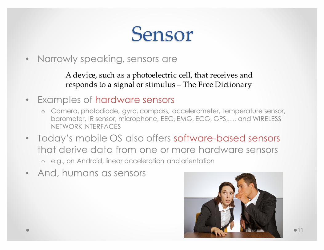
Sensor• Narrowly speaking, sensors are
• Examples of hardware sensorso Camera, photodiode, gyro, compass, accelerometer, temperature sensor,
barometer, IR sensor, microphone, EEG, EMG, ECG, GPS,…, and WIRELESS NETWORK INTERFACES
• Today’s mobile OS also offers software-based sensors that derive data from one or more hardware sensorso e.g., on Android, linear acceleration and orientation
• And, humans as sensors
11
A device, such as a photoelectric cell, that receives and responds to a signal or stimulus – The Free Dictionary

Wireless Interfaces as Sensors• Not such a radical idea• Positioning
o Global positioning system (GPS)o Cellular e-911o iBeacon
• Proximityo NFCo RFID
• Otherso Motion detectiono Gesture recognition
12
La distancia entre un iBeacon y el dispositivo receptor está categorizada dentro de 3 rangos distintos:
• Inmediato: menos de 50cm.• Cerca: aproximadamente entre 50cm y 2,5m.• Lejos: más o menos entre 2,5m y 30/50m, dependiendo de parede y de la potencia de emisión y otros
muchos factores.
Estos rangos se definen para notificar cambios de zona a las aplicaciones cuando estas están en background. En foreground es posible obtener la distancia exacta a la baliza midiendo el nivel de señal que nos llega y comparándolo con el valor de señal a 1m que va encapsulado en el paquete que recibimos de la baliza.
iBeacon for dummies

Wireless Sensors: Why, How and Limitations
13
R: reflection
D: diffraction -- a modification which light undergoes especially in passing by the edges of opaque bodies or through narrow openings
S: scattering -- obstacle << wave length
λ = C / fEx: 3e8/2.4e9 = 12.5cm

Wireless Link CharacteristicsDifferences from wired link ….
o decreased signal strength over distance: radio signal attenuates as it propagates through matter (path loss)
o interference from other sources: standardized wireless network frequencies (e.g., 2.4 GHz) shared by other devices (e.g., phone); devices (motors) interfere as well
o multipath propagation: radio signal reflects off objects ground, arriving ad destination at slightly different times
… make communication across (even a point-to-point) wireless link much more “difficult”

Radio Propagation Models
How to characterize the signal at the receiver?-‐‑Transmitter, receiver, environment, time-‐‑ Large scale, small scale
Propagation Models • Large scale models predict behavior averaged
over distances >> wave length λ=c/fo Function of distance & significant environmental features, roughly
frequency independento Breaks down as distance decreaseso Useful for modeling the range of a radio system and rough capacity
planning
• Small scale (fading) models describe signal variability on the scale of λo Multipath effects (phase cancellation) dominate, path attenuation
considered constanto Frequency and bandwidth dependento Focus is on modeling “Fading”: rapid change in signal over a short
distance or length of time

Large-‐‑scale Models• Path loss models
o Free spaceo Log-distanceo Log-normal shadowing
• Outdoor modelso “2-Ray” Ground Reflection modelo Diffraction model for hilly terrain
• Indoor models
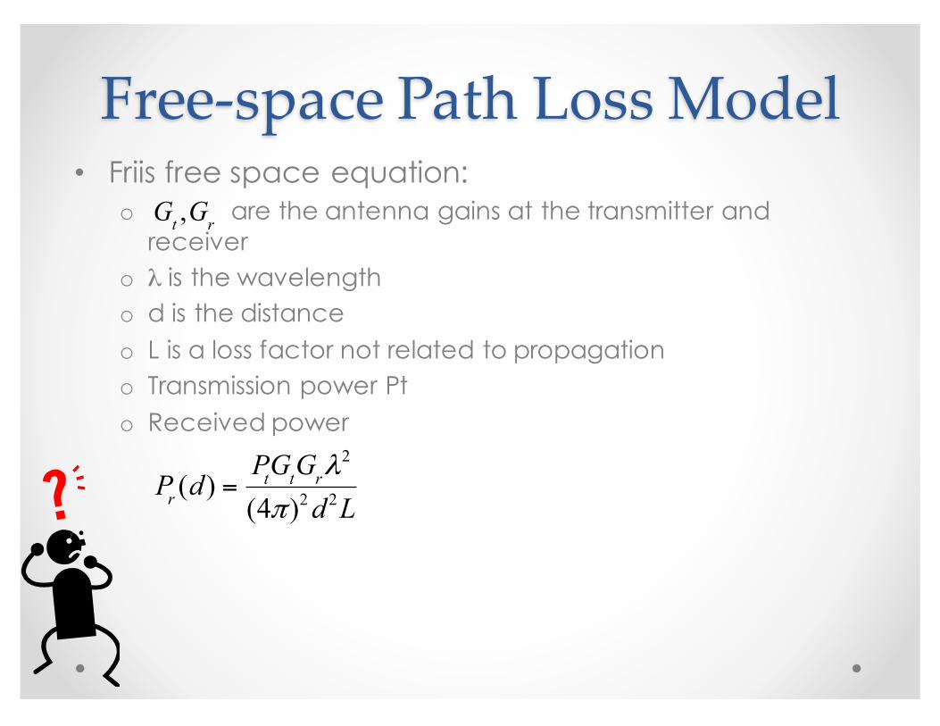
• Friis free space equation:o are the antenna gains at the transmitter and
receivero λ is the wavelengtho d is the distanceo L is a loss factor not related to propagationo Transmission power Pto Received power
Pr (d) =PtGtGrλ
2
(4π )2 d 2L
Gt ,Gr
Free-‐‑space Path Loss Model

• Friis free space equation:o are the antenna gains at the transmitter and
receivero λ is the wavelengtho d is the distanceo L is a loss factor not related to propagationo Transmission power Pt
o Received power
Pr (d) =PtGtGrλ
2
(4π )2 d 2L
Gt ,Gr
Free-‐‑space Path Loss Model
Er ( f , t) =α cos2π f (t − d / c)
dPr (d)∝ Er
2 ( f , t)
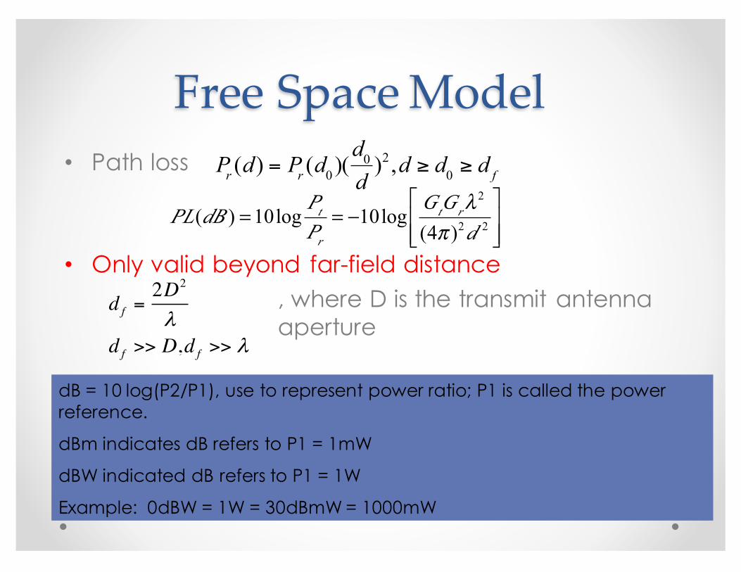
Free Space Model• Path loss
• Only valid beyond far-field distance, where D is the transmit antenna aperture
PL(dB ) =10logPtPr
= −10logGtGrλ
2
(4π )2d 2
⎡
⎣⎢⎢
⎤
⎦⎥⎥
Pr (d) = Pr (d0 )(
d0
d)2 ,d ≥ d0 ≥ d f
dB = 10 log(P2/P1), use to represent power ratio; P1 is called the power reference.
dBm indicates dB refers to P1 = 1mW
dBW indicated dB refers to P1 = 1W
Example: 0dBW = 1W = 30dBmW = 1000mW
d f =2D2
λd f >> D,d f >> λ

Example• Far field distance for an antenna with maximum
dimension of 1m and operating freq of 900MHz
• Consider a transmitter producing 50w of power and with a unity gain antenna at 900MHz. What is the received power in dBm at a free space distance of 100? What about 10Km? (assume L =1)
d f =2D2
λ= 23×108 / 900 ×106
= 6m
Pt =10 log(50 ×103) = 47dBm
Pr (100) =PtGtGrλ
2
(4π )2d 2L= 3.5×10⁻³mW = −24.5dBm
Pr (10km) = −24.5− 20 log(100) = −64.5dBm

Log-‐‑distance Path Loss Model
• Log-distance generalizes path loss to account for other environmental factors
• Choose a d0 in the far field.• Measure PL(d0)• Take measurements and derive β empirically
PL(d)[dB] = PL(d0 )+10β log(d / d0 )

Log-‐‑normal Shadowing• Shadowing occurs when objects block light of sight
(LOS) between transmitter and receiver
PL(d)[dB] = PL(d) + Xσ = PL(d0 ) +10β log( d
d0
) + Xσ
Xσis a zero-mean Gaussian distributed random variable (in dB) with standard deviation σ (also in dB)

Small-‐‑scale Fading• Factors that contribute to small-scale fading
o Multi-path propagation -- phase cancellation etc.o Speed of the mobile -- Dopler effecto Speed of surrounding objectso The transmission bandwidth of the signal wrt bw of the channel

Multipath Causes Phase Difference
Green signal travels 1/2λ farther than Yellow to reach receiver, who sees Red. For 2.4 GHz, λ (wavelength) =12.5cm.
Direct path

Reflecting wall, fixed antenna
Er ( f , t) =α cos2π f (t − r / c)
r− α cos2π f (t − (2d − r) / c)
2d − r
Phase difference: Δθ = 4π fc
(d − r)+π
Transmit antenna
walld
r
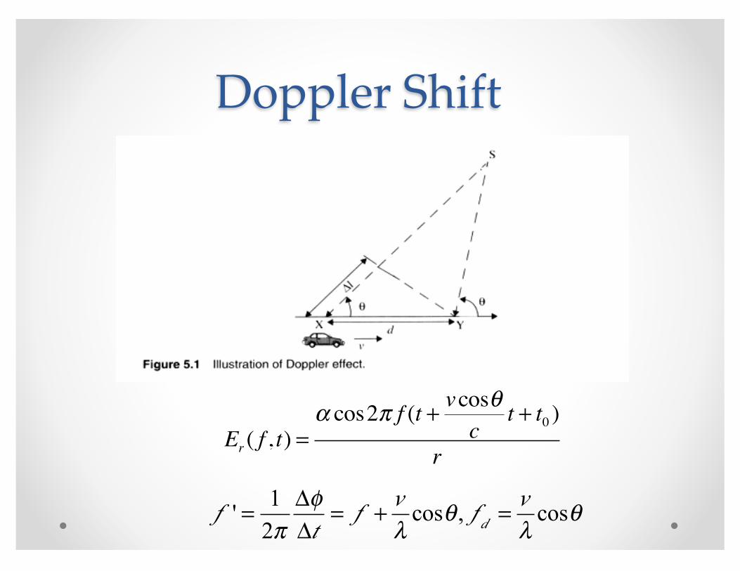
Doppler Shift
f ' = 12π
ΔφΔt
= f + vλcosθ , f d = v
λcosθ
Er ( f , t) =α cos2π f (t + vcosθ
ct + t0 )
r

Example: Police Radar
freflected − ftransmitted = Δf =2vt argetλ
f = 900MHz,λ = 0.333m,v = 60Km / hrΔf =100Hz
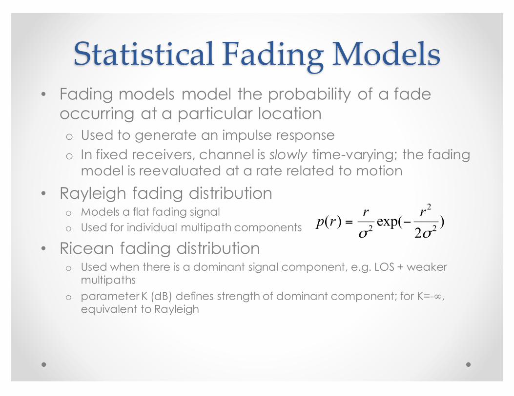
Statistical Fading Models• Fading models model the probability of a fade
occurring at a particular locationo Used to generate an impulse responseo In fixed receivers, channel is slowly time-varying; the fading
model is reevaluated at a rate related to motion
• Rayleigh fading distributiono Models a flat fading signalo Used for individual multipath components
• Ricean fading distributiono Used when there is a dominant signal component, e.g. LOS + weaker
multipathso parameter K (dB) defines strength of dominant component; for K=-∞,
equivalent to Rayleigh
p(r) = r
σ 2 exp(− r 2
2σ 2 )

Wireless Sensors Can …• Positioning
o Global positioning system (GPS)o Cellular e-911o iBeacon
• Proximityo NFCo RFID
• Otherso Motion detectiono Gesture recognition
30
✔
✔
✔

Trilateration with Wireless Signals• If we know distances to known anchors (e.g, WLAN APs,
cellular tower) exactlyo Trilateration à location in 2D
• In reality, o Anchors location may not be known exactlyo No actual ranging measurements
• Instantaneous measurements fluctuate• Path loss exponent unknown/changes• Antenna gain not known
o The circles may not intersect
31
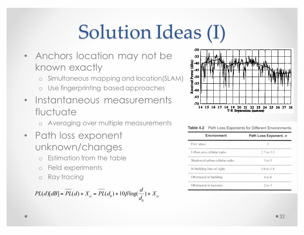
Solution Ideas (I)• Anchors location may not be
known exactlyo Simultaneous mapping and location(SLAM) o Use fingerprinting based approaches
• Instantaneous measurements fluctuateo Averaging over multiple measurements
• Path loss exponent unknown/changeso Estimation from the tableo Field experimentso Ray tracing
32
PL(d)[dB] = PL(d) + Xσ = PL(d0 ) +10β log( d
d0
) + Xσ

Solution Ideas(II)• Antenna gain unknown
o Treat as a variable to solveo Subtract out
• The circles may not intersecto Minimizing square errors
where d1, d3, d3 are distances estimation from the path loss model, (x1, y1), (x2, y2), (x3, y3) are the anchor locationso Can implement using an exhaustive search
33
arg! ,!!"# !! − !! − ! !+ !! − ! !!+ !! − !! − ! !+ !! − ! !
!
+ (!! − !! − ! !+ !! − ! !)! !

Algorithm Sketch (WiFi)
34
Scan Beacon Messages<MAC Addr, RSS>
Averaging Consecutive Scans
<RSS1, RSS2, …, RSSn>
Note: need to distinguish virtual APs
<RSS1-‐‑RSSn, RSS2 –RSSn, …, RSSn-‐‑1-‐‑RSSn>
Remove effects of antenna gains
<Δ1, Δ2, …, Δn-‐‑1>Best
match?
GuessedLocation
AP locations, path loss co-‐‑efficient
Estimated Location, Confidence
Confidence can be computed using the log-‐‑normal model assuming independent distributions
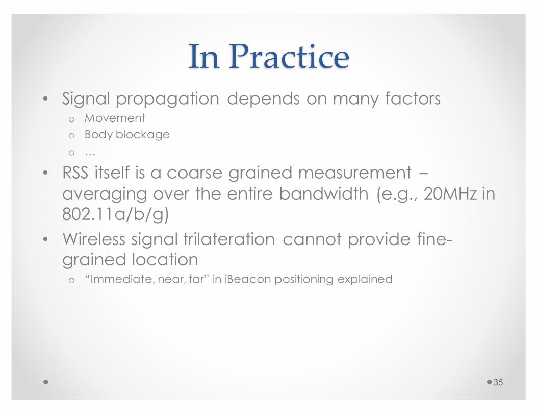
In Practice• Signal propagation depends on many factors
o Movemento Body blockageo …
• RSS itself is a coarse grained measurement –averaging over the entire bandwidth (e.g., 20MHz in 802.11a/b/g)
• Wireless signal trilateration cannot provide fine-grained locationo “Immediate, near, far” in iBeacon positioning explained
35

Wireless Fingerprinting• Trilateration approaches face difficulties in 1) locations of APs,
and 2) RSS not a good measure for distance• Alternatively, we can treat wireless signal propagation as a
blackbox and associate RF signal measurements as “fingerprints” at locations
36

Algorithm Sketch (WiFi)
Implementation notes:• For both the site survey and online phases, need to
take averages of multiple RSS readings respective to the same AP
• Can use <Δ1, Δ2, …, Δn-1> as fingerprints to mitigate device heterogeneity
37
Site Survey TrainingModelf-‐‑1: FP-‐‑> <x,y, z>
new RSS readings
Location

Implementation Notes• The training phase:
o Can be as simple as just setting up a lookup tableo Or, performing regression/function fitting to derive the mapping f: <x, y,z>
à FP (more on regression later)
• In the online phase, o Table lookupo Solving an optimization problem or using an exhaustive searcho Be aware of missing AP data
38
Incomplete data
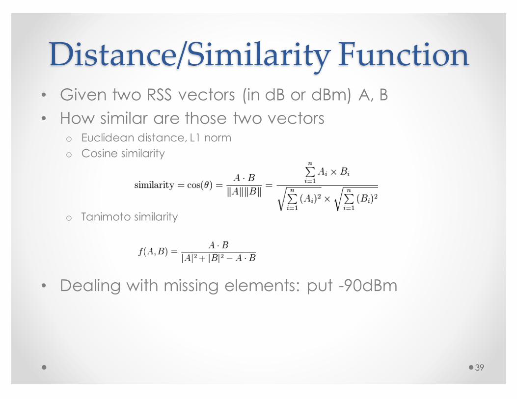
Distance/Similarity Function• Given two RSS vectors (in dB or dBm) A, B• How similar are those two vectors
o Euclidean distance, L1 normo Cosine similarity
o Tanimoto similarity
• Dealing with missing elements: put -90dBm
39
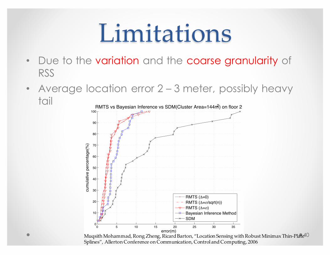
Limitations• Due to the variation and the coarse granularity of
RSS• Average location error 2 – 3 meter, possibly heavy
tail
400 5 10 15 20 25 30 35
0
10
20
30
40
50
60
70
80
90
100RMTS vs Bayesian Inference vs SDM(Cluster Area=144m2) on floor 2
error(m)
cum
ulat
ive
perc
enta
ge(%
)
RMTS (∆=0)RMTS (∆=σ/sqrt(n))RMTS (∆=σ)Bayesian Inference MethodSDM
MuqsithMohammad, Rong Zheng, RicardBarton, “Location Sensing with Robust MinimaxThin-‐‑Plate Splines”, AllertonConference on Communication, Control and Computing, 2006

Fine-‐‑grained RF Fingerprints• 802.11 a/g/n implements OFDM
o Wideband channel divided into subcarriers
• Intel 5300 card exports frequency response per subcarrier
41
Frequency subcarriers
1 2 3 4 5 6 7 8 9 10 39 48
cluster2
cluster2
Higher resolutionbut higher variability too
Sen, S., Radunovic, B., Choudhury, R. R., Minka, T., "ʺYou are facing the Mona Lisa: Spot Localization Using PHY Layer Information"ʺ, MobiSys 2012

Motion Detection• Channel state information (CSI) may not be suitable
for indoor positioning but can be useful in motion detection and gesture recognitiono Presence, movement of people in the environmento Changes in gesture/posture
• Can be used in device free scenarios (also called radio tomographic)
42

Take-‐‑home Messages• RF signal power/phase à Channel à position
(device-based), motion, gesture (device-free)• Didn’t cover direct time of flight (ToF), angle of
arrival (AoA) based methodso GPSo WiZ
• Compared to visible lights and IR, no need for line of light in RF is both a curse and a blesso Can be used to detect motion behind wallso Signal propagation is not easily confined
• Issues that will be addressed in later part of the courseo Movement is more than a collection of positions -- Bayesian filteringo Moved or not? How many people? -- Classification
43

Further Reading• T S Rappaport, Chapter 4, Wireless Communications
Principles And Practice
44