separated longitudinal drive-train for wheel-loaders
TRANSCRIPT
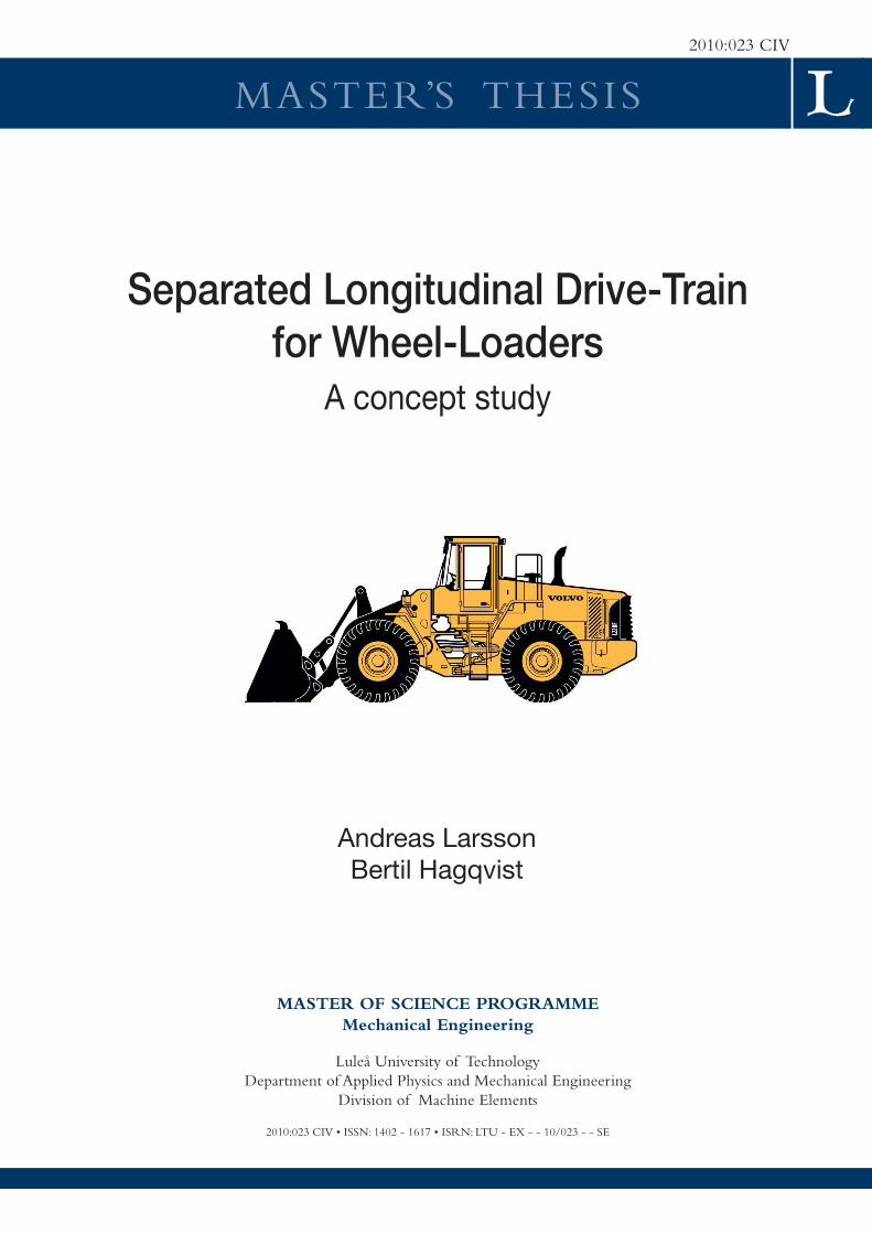
MASTER’S THESIS2010:023 CIV
Universitetstryckeriet, Luleå
Andreas LarssonBertil Hagqvist
Separated Longitudinal Drive-Trainfor Wheel-Loaders
A concept study
MASTER OF SCIENCE PROGRAMME Mechanical Engineering
Luleå University of Technology Department of Applied Physics and Mechanical Engineering
Division of Machine Elements
2010:023 CIV • ISSN: 1402 - 1617 • ISRN: LTU - EX - - 10/023 - - SE

1
Preface
This thesis work marks, after 20 weeks of hard labour, the end of our studies at the Master of Science programme in Mechanical Engineering at Luleå University of Technology. These 20 weeks at Volvo Construction Equipment in Eskilstuna has been an interesting experience where we have had a glimpse of the life after graduation and a possibility to put our theoretical knowledge into practice.
First of all we would like to thank Lena Brattberg Norman for giving us a chance to conduct our thesis work at the Component Technology department and for the warm welcome we received.
Furthermore we would like to tank our supervisors Joakim Lundin and Ralf Nordström for their invaluable help and selfless support at all times. Their immense knowledge, both in specific areas and of the company with its employees has always helped us to get answers for our questions. Special thanks also to everyone else at Volvo Construction Equipment who has taken time to help us during our thesis work.
At Luleå University of Technology we would like to send thanks to our examiner Pär Marklund whose constructive feedback and report writing knowledge has been of great help. Also, his relaxed attitude and genuine interest for technology is always an inspiration and makes the subject reachable.
Finally, we would like to thank Christian Liljendahl and Lukas Edvardsson who have taken care of two lost souls in Eskilstuna.
Andreas Larsson Bertil Hagqvist Eskilstuna, January 2010

2

3
Abstract
This thesis work is done in cooperation with Volvo Construction Equipment, a business area within the Volvo Group, which is one of the world’s leading manufacturers of construction equipment such as wheel-loaders, excavators, articulated haulers, road development equipment and compact equipment.
Concurrently with increasing fuel costs and environmental demands, such as CO2 emissions, ever increasing demands are placed on the producers to manufacture fuel efficient construction equipment. In order to maintain a leading market position Volvo Construction Equipment continuously need to improve the design of future generation construction equipment including fuel efficient high performing drive-train components.
The traction, performance and efficiency of all-wheel drive vehicles are strongly influenced by the way the differentials operate. In a wheel loader there are currently no differential between the front and rear axle but a rigid connection. This results in a wind-up torque build-up in the drive-train which contributes to losses and adds additional stress to the components.
The aim of this thesis is to investigate the feasibility and propose a mechanical design for separating the longitudinal drive-train for a large wheel-loader. The solution is to be optimised based on demands such as size, cost, performance, efficiency and controllability.
To reach the aims a pre-study was performed where the current drive-train design was studied as well as the competitors and related technology. The pre-study showed that few competitors have solutions for this problem, and those that does, have a very basic design and function. Problems with the current design were investigated together with possible problems and gains from a future design change. This showed that a fuel efficiency gain can not be secured with the data available and that a separation of the drive-train can not decrease the most critical stresses in the drive-train without causing a negative impact on the vehicles retardation ability, using the brake setup of today.
The work also resulted in a number of concepts for mechanical designs of a separated longitudinal drive-train as well as a concept evaluation performed together with engineers at Volvo CE. For the selected concept, a planetary differential with a wet-clutch differential lock, reasonableness calculations and drawings was also produced. Furthermore, the thesis shows that it is possible to fit such a solution in the current transmission housing without any drastic changes.

4

5
Table of contents 1. Introduction ................................................................................................................................9
1.1. Project background................................................................................................................9 1.2. Project outline .......................................................................................................................9 1.3. Aim and scope.....................................................................................................................10
2. Problem description .................................................................................................................11 2.1. Wheel-loader applications...................................................................................................11 2.1. Current design .....................................................................................................................11 2.2. Problem areas ......................................................................................................................12 2.3. Problem statement ...............................................................................................................12
3. Method ......................................................................................................................................13 4. Concept study ...........................................................................................................................14
4.1. Competitors and related technology....................................................................................14 4.2. Function analysis.................................................................................................................15 4.3. Definition of prerequisites...................................................................................................15 4.4. Concept break-down ...........................................................................................................16
4.4.1. Differential ...................................................................................................................16 4.6.2. Axle disconnect ............................................................................................................17 4.4.3. Dog-clutch....................................................................................................................17 4.4.4. Multi-plate wet clutch ..................................................................................................18
4.5. Assessment of potential benefits/drawbacks .......................................................................19 4.5.1. Fuel saving potential ....................................................................................................19 4.5.2. Reduction of component stresses .................................................................................19 4.5.3. Vehicle handling ..........................................................................................................22
4.6. Concept evaluation and selection ........................................................................................22 5. Detailed design..........................................................................................................................23
5.1. Design layout ......................................................................................................................23 5.2. Sub-systems.........................................................................................................................23
5.2.1. Wet clutch ....................................................................................................................23 5.2.2. Differential ...................................................................................................................26 5.2.3. Dog-clutch....................................................................................................................26 5.2.4. Bearings........................................................................................................................28 5.2.5. Hydraulic system..........................................................................................................29
5.3. Final design .........................................................................................................................30 5.4. Estimation of production cost..............................................................................................31 5.5. Suggestion of control strategy.............................................................................................32
6. Conclusions and recommendations ........................................................................................34 7. List of references ......................................................................................................................35 List of appendices
APPENDIX A – Fuel saving potential APPENDIX B – Separated drive-train – driving dynamics test APPENDIX C – Concept evaluation APPENDIX D – Bearing dimensioning APPENDIX E – Dog-clutch dimensioning APPENDIX F – Differential gears calculation result APPENDIX G – FE-analysis of complex components APPENDIX H – Spline dimensioning APPENDIX I – Screw joints APPENDIX J – Early ideas APPENDIX K – Drawings

6
7
Nomenclature Variables a Acceleration [m/s2] c Specific heat capacity [J/kgK] d Brake distribution ratio [-] F Force [N] g Gravity constant [m/s2] h Height [m] J Inertia [kgm2] k Spring constant [N/m] L Length [m] M Moment [Nm] m Mass [kg] N Gear ratio [-] n Number [-] p Pressure [Pa] Q Heat accommodation [J] R Radius [m] r Differential distribution ratio [-] s Distance [m] T Temperature [°C] v Velocity [m/s] μ Coefficient of friction [-] φ Angle [rad] ω Rotational speed [rad/s] ρ Density [kg/m3]
Subscripts AFF Available friction front AFR Available friction rear axle Wheel axle bp Balance piston br Brake c Clutch cbo Clutch during break-out cm Center of mass dc Dog-clutch FF Friction front FR Friction rear f Friction interfaces fd Friction disc fi Friction disc inner fo Friction disc outer g Ground max Maximum value mfb Maximum front brake N Normal NF Normal front NR Normal rear oil Oil p Piston pi Piston inner

8
po Piston outer ps Propeller shaft rot Rotation rs Rear shaft s Screws sp Spring st Stroke stall During stall tire Wheel-loader tire wb Wheel base

9
1. Introduction
This thesis work is done in cooperation with Volvo Construction Equipment, a business area within the Volvo Group, which is one of the world’s leading manufacturers of construction equipment such as wheel loaders, excavators, articulated haulers, road development equipment and compact equipment. Production facilities are located in Europe, Asia, North America and Latin America. The turnover for 2007 reached SEK 53 billion. The number of employees is approximately 16 000. The Component Division, at which this thesis work is done, develops drive-trains to Volvo’s construction machinery such as their wheel-loaders. Engines, transmissions, axle systems and vehicle electronics are the main components being developed at this division located in Eskilstuna. 1.1. Project background
The drive-train setup of all all-wheel drive vehicles is crucial for its traction, efficiency and performance. In Volvo’s wheel-loaders there is currently a rigid connection between the front and rear axle, no differential or other type of connection that allows the axles to rotate at different speeds is present. This results in wind-up torque build-up in the drive-train which contributes to losses and adds additional stress to the components. The drive-train setup also affects vehicle stability, handling and brake performance. Therefore, in order to improve fuel efficiency, durability and traction of the Volvo wheel-loaders the potential contributions from a separated longitudinal drive-train need to be studied. In Figure 1 below the wheel-loader drive-train setup can be seen.
Figure 1. Wheel-loader drive-train.
1.2. Project outline
According to the company’s directives the following activities will be performed during the thesis work
• Literature review and competitor studies • Definition of design pre-requisites • Concept generation • Concept selection • Detailed development of selected concept • Estimation of production cost • Writing of technical report • Suggestion of continued work • Presentation of the work at Volvo CE and Luleå University of Technology

10
1.3. Aim and scope
To reduce the extension of the project it is limited to only one transmission, HTE-305, with performance and space requirement from existing transmissions. The work is also limited to deal with the mechanical development. Simulations concerning efficiency and performance are carried out by Volvo engineers.
The aim of this thesis is to analyze needs, identify critical areas and produce a number of concepts for an improved wheel-loader transmission, with respects to energy efficient propulsion, drivetrain component stress and torque distribution. Also, a detailed design of one of these concepts suitable for a technology demonstrator is aimed to be performed together with a compilation of recommendations for continued work.

11
2. Problem description
This chapter presents the work environment of the wheel-loader as well as the current design and the problems that occur because of this design. The chapter is ended with a formulation of the problem.
2.1. Wheel-loader applications
The Volvo loaders that this master thesis aims for are mainly used in extreme environments
and heavy duty applications. Their purpose is to lift and transport gods, often gravel from a pile to a hauler for example. The ground is usually slippery and rough, and with heavy load in the bucket the weight on the rear axle is a fraction of the weight on the front one. This places high demands on the drive-train to distribute the right amount of torque to utilize all tractive force available. 2.1. Current design
Most Volvo wheel-loaders are designed to have equal distance, X, from the front and rear axle to the articulation joint, see Figure 2. This setup makes the curve radius, R, and the travelled distance equal for both axles when cornering, which has made a solution whit a rigid shaft between the front and rear axle possible. The rigid shaft is placed in the transmission and connects the front and rear shaft to each other and distributes torque from the transmission to them.
Figure 2. Wheel-loader geometry.
Wheel-loaders from Volvo have a dog-clutch for differential locking in the front axle and an
optional limited slip differential in the rear axle. The rear axle can oscillate 15 degrees in each direction to make all wheels obtain ground contact on broken ground.
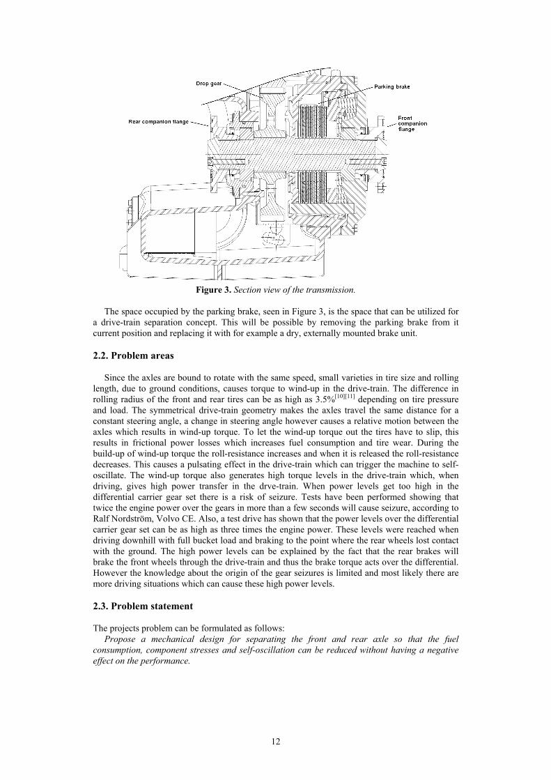
With the current design the longitudinal drive-train is rigid and no locking device is needed between the axles. In Figure 3 a section view of the current transmission can be seen. It shows the lower part of the transmission where this projects design space lie.
12
Figure 3. Section view of the transmission.
The space occupied by the parking brake, seen in Figure 3, is the space that can be utilized for
a drive-train separation concept. This will be possible by removing the parking brake from it current position and replacing it with for example a dry, externally mounted brake unit.
2.2. Problem areas
Since the axles are bound to rotate with the same speed, small varieties in tire size and rolling length, due to ground conditions, causes torque to wind-up in the drive-train. The difference in rolling radius of the front and rear tires can be as high as 3.5%[10][11] depending on tire pressure and load. The symmetrical drive-train geometry makes the axles travel the same distance for a constant steering angle, a change in steering angle however causes a relative motion between the axles which results in wind-up torque. To let the wind-up torque out the tires have to slip, this results in frictional power losses which increases fuel consumption and tire wear. During the build-up of wind-up torque the roll-resistance increases and when it is released the roll-resistance decreases. This causes a pulsating effect in the drive-train which can trigger the machine to self-oscillate. The wind-up torque also generates high torque levels in the drive-train which, when driving, gives high power transfer in the drve-train. When power levels get too high in the differential carrier gear set there is a risk of seizure. Tests have been performed showing that twice the engine power over the gears in more than a few seconds will cause seizure, according to Ralf Nordström, Volvo CE. Also, a test drive has shown that the power levels over the differential carrier gear set can be as high as three times the engine power. These levels were reached when driving downhill with full bucket load and braking to the point where the rear wheels lost contact with the ground. The high power levels can be explained by the fact that the rear brakes will brake the front wheels through the drive-train and thus the brake torque acts over the differential. However the knowledge about the origin of the gear seizures is limited and most likely there are more driving situations which can cause these high power levels. 2.3. Problem statement The projects problem can be formulated as follows:
Propose a mechanical design for separating the front and rear axle so that the fuel consumption, component stresses and self-oscillation can be reduced without having a negative effect on the performance.

13
3. Method
The first stage of the project is the pre-study where information is gathered in different areas and purposes through literature studies, patent studies, interviews and by searching in internal documents and test reports. Different solutions for similar technologies are investigated to get a broader view of the subject. A study of the current design is also crucial for understanding its weaknesses and strengths.
A function analysis is performed, based on the information retrieved during the pre-study, to get a better grip of the actions that are needed for reaching the target and accomplishing increased customer values.
To pin point the demands on the new drive-train the prerequisites are defined for all measurable properties. The properties that have known demands that have to be fulfilled are governed by limits that they have to obtain. Other properties are governed by aims to show in which directions they have to go to be competitive.
The next phase is the concept generation where different concept and combination of concepts are generated through different processes and with the prerequisites in mind. Concepts that do not stand a chance to reach the limits of the prerequisites or are way off the aims are ruled out immediately, while reasonable concepts are kept for the concept refinement.
In the concept refinement phase all concepts are refined to be as competitive as possible for the concept selection. All concepts are looked upon one by one and the goal is to make every concept optimised, even if there are other concepts that seam to be better solutions. This is done so that no personal opinions should effect the concept selection.
Evaluation of the concepts will be done through evaluation matrixes and discussions with engineers at Volvo. The benefits and the drawbacks are pin pointed for each concept and weighted to get the relative relation between them.
The concept selection will be made together whit Volvo CE engineers, based on the concept evaluation, to find the concept best suited for Volvo CE.
A first design layout will be done for the chosen concept so that it fits in the transmission and all parts work together as they should. This will form the basis of the definition of sub-systems.
To structure the development work the concept is divided into sub-systems with different functions. The sub-systems are classified after how critical they are so the most critical sub-systems are detected and looked into first.
For solving some of the sub-systems, available components at Volvo and other suppliers might be used, that would save time and production cost for a demonstrator. These components will be looked up and evaluated.
The other sub systems are then developed and designed to make the usage of the available components possible and to fulfil their purpose. This phase will include calculations and analysis to design and verify the functions of each sub-system.

14
4. Concept study
This chapter contains a summary of competitor technology and related technology where the competitors’ solution to the problem and solutions to similar problems in other business areas are dealt with. The prerequisites are presented in this part of the report together with the function analysis. The solution span is defied in the concept break-down as the possible combinations of important sub-systems witch are also described more in detail under this subheading. Different, possible drawbacks and benefits of the different solutions are discussed and evaluated, the solutions are narrowed down to four concepts and from these one is selected as the final concept. 4.1. Competitors and related technology
Most competitors have the same solution, regarding the longitudinal drive-train, as Volvo have in their wheel-loaders. John Deere, who purchases their transmissions from ZF, has a solution with rear axle disconnect for their smaller wheel-loaders (5-8 tons capacity). That solution is an optional clutch package which is bolted on to the existing transmission. The clutch is a solenoid engaged dog-clutch, see Figure 4, and can only be operated while standing still. John Deere has also had a solution with front axle disconnect for the smaller machines but this is no longer available.
Figure 4. John Deere's rear axle disconnect. [I]
Volvo’s first articulated wheel loaders LM 845/846, manufactured between the years 1972
and 1979, had a disconnectable rear axle. The disengagement was controlled by a leaver in the driver cabin. In earlier rear wheel steered models, LM 640/840, also had a disconnectable rear axle and this when shifting into transport gear. In both types of machines the engagement/disengagement was performed by a dog-clutch. As of the 4300 model Volvo removed the separated longitudinal drive train and has not had such a solution since then.
In the automotive industry there are many different layouts of all wheel drive systems. There are systems with engageble front or rear axle and systems with longitudinal differential combined with clutches of different types. The trend within this industry is that manually controlled dog-clutches are replaced with electronically controlled wet clutches used together with the traction control system. An example of an all wheel drive system with engageble rear axle can be seen in Figure 5.

15
Figure 5. Schematic drive-train of modern all-wheel drive system.
Volvo’s articulated haulers use a longitudinal differential combined with a dog-clutch operated
either manually or automatically. Current development project are however investigating the possibility of replacing the dog-clutch with a wet-clutch because of its favourable engage/disengagement properties.
4.2. Function analysis
The purpose of the function analysis is to find the action areas for the longitudinal drive-train concepts. To obtain the main function on the first level the sub-functions of the second level must be fulfilled, and to obtain these the sub-functions on the third level must be fulfilled and so forth.
In a concept for a new longitudinal drive-train one must fulfil the customer demands. To meet the demands there are some critical areas to be considered and these are solved by the actions. This is done in the function analysis diagram in Figure 6.
Off-road ability Fuel consumptionDurability Comfort
Avoid wheel-slip
Supply full torque for both
axles
Limit speed difference between axles
Avoid high unwanted power levels in the
drive-trainReduce roll resistance Avoid trigging
self-oscillations No driver
interference
Autonomous system
Separate rotational speeds of axles
Longitudal drive-train
Customer values
Actions
Critical areas
Figure 6. Function analysis diagram. 4.3. Definition of prerequisites
The requirements are governed by both limits and aims. Some properties has certain demands
that has to be fulfilled, these properties are governed by limits. All concepts have to fulfil all the properties with a limit. Most limits are inherited from the current drive-train design. Other properties may not have a specific limit but are still important. These properties are governed by aims. The aim point in which direction the property needs to go to be competitive in the concept selection. In Table 1 the limits and aims for each property can be seen.

16
Table 1. List of requirements. Property Limit Aim Unit Torque capacity front axle 12800 [Nm] Torque capacity rear axle 9000 [Nm] Life L10 >10000 [hours] Degree of automation 100% [-] Parking brake VCE demand[12] [-] Production cost Minimize [SEK/piece
] Wind-up torque < Current Minimize [Nm] Efficiency > Current Maximize [-] Mounting dimensions = Current [m3] Service interval > Current [hours] Weight Minimize [kg] Engagement time Minimize [s] Number of parts/complexity Minimize [-]
The front axle torque capacity in Table 1 is determined by the maximum torque delivered from
the torque converter, the stall torque. To determine the needed torque capacity of the rear axle the weight on the rear axle when crowding, i.e. lifted front axle, and the obtainable friction of the wheels are used as limiting factors. The mounting dimension requirement refers to the placement of the companion flanges and that the transmission housing is unchanged.
4.4. Concept break-down
To get an overview of the realistic solution space a break-down of the solutions are
performed, Figure 7.
Differential Axle disconnect
Front axle disconnect Rear axle disconnect Front/Rear axle disconnect
Wet clutch Wet clutchWet clutchWet clutch Dog clutch Dog clutch Dog clutchDog clutch
Differential lock
Axle separation
Figure 7. Axle separation break-down.
Removing the wind-up torque is only possible by separating the axles and this can be done by
either using a differential or by disconnecting one axle. To keep the performance of today’s solution one has to be able to lock the differential or connect the disconnected axle when the traction is low and/or high amount of tractive force is needed. This can be achieved by using either a dog-clutch or a wet clutch to lock the drive-train. In the axle disconnect case you obviously can have a solution which can disconnect/connect either of the axles. This can seem unnecessarily complicated but there is such a solution available on the market which is fully automatic and uses one dog-clutch for each shaft, called NoSpin™ or Detroit locker™.
4.4.1. Differential
Since the differential distributes torque between the axles with a fixed distribution ratio[3] the available traction for one axle will determine the available tractive force for the vehicle, depending on the distribution ratio. This ratio can be selected to fit the axle weight distribution to obtain as high tractive force as possible at conditions where the coefficient of friction between tires and ground is the same for all wheels. For wheel-loaders the weight distribution between the axels shifts depending on the load. This, and the fact that the friction coefficient between tire and
17
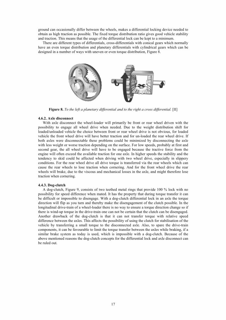
ground can occasionally differ between the wheels, makes a differential locking device needed to obtain as high traction as possible. The fixed torque distribution ratio gives good vehicle stability and traction. This means that the usage of the differential lock can be kept to a minimum.
There are different types of differentials, cross-differentials with conical gears which normally have an even torque distribution and planetary differentials with cylindrical gears which can be designed in a number of ways with uneven or even torque distribution, Figure 8.
Figure 8. To the left a planetary differential and to the right a cross differential. [II]
4.6.2. Axle disconnect
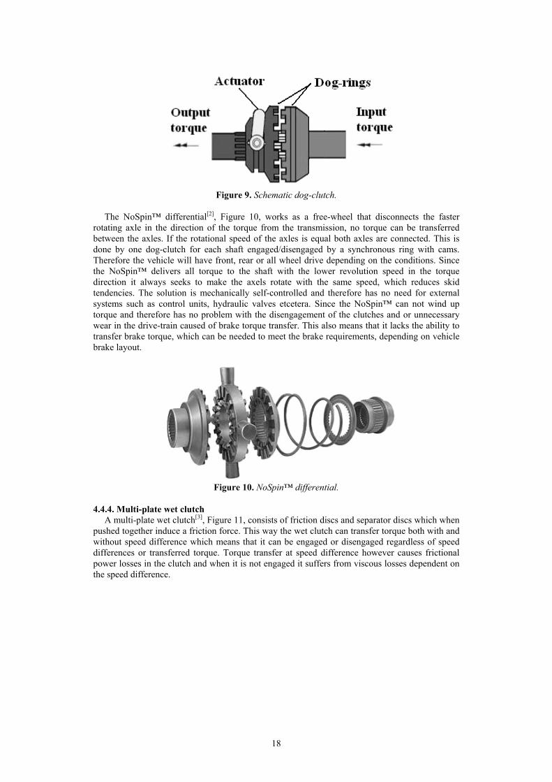
With axle disconnect the wheel-loader will primarily be front or rear wheel driven with the possibility to engage all wheel drive when needed. Due to the weight distribution shift for loaded/unloaded vehicle the choice between front or rear wheel drive is not obvious, for loaded vehicle the front wheel drive will have better traction and for un-loaded the rear wheel drive. If both axles were disconnectable these problems could be minimized by disconnecting the axle with less weight or worse traction depending on the surface. For low speeds, probably at first and second gear, the all wheel drive will have to be engaged because the tractive force from the engine will often exceed the available traction for one axle. In higher speeds the stability and the tendency to skid could be affected when driving with two wheel drive, especially in slippery conditions. For the rear wheel drive all drive torque is transferred via the rear wheels which can cause the rear wheels to lose traction when cornering. And for the front wheel drive the rear wheels will brake, due to the viscous and mechanical losses in the axle, and might therefore lose traction when cornering. 4.4.3. Dog-clutch
A dog-clutch, Figure 9, consists of two teethed metal rings that provide 100 % lock with no possibility for speed difference when mated. It has the property that during torque transfer it can be difficult or impossible to disengage. With a dog-clutch differential lock in an axle the torque direction will flip as you turn and thereby make the disengagement of the clutch possible. In the longitudinal drive-train of a wheel-loader there is no way to ensure a torque direction change so if there is wind-up torque in the drive-train one can not be certain that the clutch can be disengaged. Another drawback of the dog-clutch is that it can not transfer torque with relative speed difference between the axles. This affects the possibility of using the clutch for stabilisation of the vehicle by transferring a small torque to the disconnected axle. Also, to spare the drive-train components, it can be favourable to limit the torque transfer between the axles while braking, if a similar brake system as today is used, which is impossible with a dog-clutch. Because of the above mentioned reasons the dog-clutch concepts for the differential lock and axle disconnect can be ruled out.
18
Figure 9. Schematic dog-clutch.
The NoSpin™ differential[2], Figure 10, works as a free-wheel that disconnects the faster
rotating axle in the direction of the torque from the transmission, no torque can be transferred between the axles. If the rotational speed of the axles is equal both axles are connected. This is done by one dog-clutch for each shaft engaged/disengaged by a synchronous ring with cams. Therefore the vehicle will have front, rear or all wheel drive depending on the conditions. Since the NoSpin™ delivers all torque to the shaft with the lower revolution speed in the torque direction it always seeks to make the axels rotate with the same speed, which reduces skid tendencies. The solution is mechanically self-controlled and therefore has no need for external systems such as control units, hydraulic valves etcetera. Since the NoSpin™ can not wind up torque and therefore has no problem with the disengagement of the clutches and or unnecessary wear in the drive-train caused of brake torque transfer. This also means that it lacks the ability to transfer brake torque, which can be needed to meet the brake requirements, depending on vehicle brake layout.
Figure 10. NoSpin™ differential.
4.4.4. Multi-plate wet clutch
A multi-plate wet clutch[3], Figure 11, consists of friction discs and separator discs which when pushed together induce a friction force. This way the wet clutch can transfer torque both with and without speed difference which means that it can be engaged or disengaged regardless of speed differences or transferred torque. Torque transfer at speed difference however causes frictional power losses in the clutch and when it is not engaged it suffers from viscous losses dependent on the speed difference.

19
Figure 11. Schematic multi-plate wet clutch.
4.5. Assessment of potential benefits/drawbacks
Here follows discussions and estimations of the most obvious benefits and drawbacks. This is
done to get a better view of the ups and downs for different solutions for the concept selection.
4.5.1. Fuel saving potential To estimate the potential fuel saving for a separated drive-train calculations have been done
based on logged vehicle data collected from Analys Matris and a fuel efficiency test, see Appendix A. The result of these calculations shows an approximate saving of 0.3%. This calculation does not consider fuel savings under 13.5 km/h, this since the fuel efficiency test was only performed in higher speeds. For the differential and axle disconnect concepts this seems logical since they probably will have to be locked at lower speeds, however the NoSpin™ will have a separated drive-train for all speeds and this could result in larger fuel savings.
4.5.2. Reduction of component stresses
The additional component stress, mainly in the differential carrier gear sets (crown wheel - pinion) of the axles, caused by wind-up torque will be considerably reduced with a separated drive-train in higher speeds. In lower speeds the power transfer over the gears due to wind-up torque is quite low and therefore does not cause as much component stress. The highest power levels over the gear sets occur when brake torque is transferred from the rear axle to the front axle through the drive-train. To determine whether this torque transfer is needed or not a calculation of the retardation capacity with separated drive-train was made using a free body diagram of the wheel-loader during braking in forward motion which can be seen in Figure 12.

20
Figure 12. Free body diagram.
Force equilibrium in X-direction gives
0=⋅++ amFF FFFR , (1) and force equilibrium in Y-direction then gives
0=⋅−+ gmFF NFNR . (2) Moment equilibrium around the point (X,Y)=(0,0) in Figure 12 gives
0=⋅⋅−⋅+⋅⋅ cmwbNFcm LgmLFham , (3) An finally the law of friction gives
NRAFR FF ⋅= μ , (4)
NFAFF FF ⋅= μ . (5)
The solution can be divided into two separate cases. The first case is that no wheel slip occurs during the braking which means that the available friction force for the rear axle, FAFR, will be the limiting factor
FRAFR FF = . (6) (6) inserted in (4) gives
NRFR FF ⋅= μ . (7)
The brake force for the front axle, FFR, will depend on the brake distribution, where the distributed amount in the rear axle, dbr and the distributed amount in the front axle, 1-dbr. This gives
FRbr
brFF F
dd
F ⋅−
=1
. (8)
(7) inserted in (8) gives

21
NRbr
brFF F
dd
F ⋅⋅−
= μ1
. (9)
(2) inserted in (3) then gives
( )wb
cmcmwbNR
LhaLLg
mF ⋅+−⋅
= . (10)
(7) and (9) inserted in (1) gives
br
NR
dmFa 1
⋅⋅−= μ . (11)
(10) inserted in (11) then gives the acceleration, a, expressed in known variables
( )cmbrwb
wbcm
hdLLLga⋅+⋅
−⋅⋅=
μμ
. (12)
This, equation (10), is only valid if ga ⋅≤ μ else ga ⋅= μ . The second case is that the rear
wheels are allowed to slip during braking and this will give the maximum retardation ability of the wheel-loader with separated drive-train. In this case the braking force in the rear axle is limited by the dynamic friction force which is assumed to be the same as the maximum available static friction force, hence equation (6) and (7) are valid for this case as well.
The brake force in the front axle is limited by the maximum brake capacity[13], Fmfb, the angular acceleration, ω’, the radius, R, and the inertia of the tires, J, so
RFF FFmfb
J'⋅−=ω
. (13)
Since the front tires doesn’t skid the angular acceleration of the tire, ω’, can be expressed by the machine acceleration, a, and the wheel radius, r.
Ra
='ω (14)
(14) inserted in (13) gives
2Ja
RFF mfbFF
⋅+= . (15)
(7) and (15) inserted in (1) gives
02 =+⋅⋅
++⋅ aRmJa
mF
mF mfbNRμ . (16)
(10) inserted in (16) then gives the acceleration, a, expressed in known variables
( )( ) 2R
LJhLm
FLLLgma
wbcmwb
mfbwbwbcm
⋅+⋅+⋅
⋅−−⋅⋅⋅=
μ
μ. (17)

22
Equation (17) is also only valid if ga ⋅≤ μ else ga ⋅= μ . In Table 2 a compilation of the calculated values of the retardation can be seen.
Table 2. Calculated retardation results L220F. Case Acceleration (Original) [m/s2] Acceleration (Separated) [m/s2] 1, Loaded -5,9 -3,4 1, Empty -7,4 -6,2 2, Loaded -5,9 -4,7 2, Empty -7,4 -6,9
The values in Table 2 are calculated for a coefficient of friction, μ=0,8. The original drive-train
has the same values for both cases since the brake capacity is not large enough to lock-up the tires. Volvo CE has brake demands of 5 m/s2 with load and 6.5 m/s2 empty. The conclusion of the results was that the braking capacity, with the brake setup of today, was insufficient for reaching the requirements without transferring torque through the drive-train. With locked rear wheels and a high coefficient of friction the demands can be barely meet however this is not recommended due to tire wear and driver safety. A test was also performed on a L150F which supported the conclusion, see Appendix B. This means that if a change of the brake setup is not done torque transfer between the axles can not be avoided when braking hard. Although the transferred torque can most probably be reduced by controlling the wet-clutches for the differential and the axle disconnect concepts. Since the NoSpin™ lacks the ability to transfer torque between the axles it will require a redesign of the brake system.
4.5.3. Vehicle handling
To observe the differences in handling a test was performed comparing the drive-train of today with the front respective the rear propeller shaft disconnected, Appendix B. The most noticeable result was that the tendency to skid increased for disconnected rear shaft, and increased even more for disconnected front shaft. Another stability problem that was found was that the rear wheels lost traction and could start to skid when braking downhill, this behaviour is equal for both front- and rear wheel drive. How the NoSpin™ and the differential would have behaved in a test like this is hard to say, but a qualified guess is that they both would have shown less tendency to skid than the axle disconnect concepts did. 4.6. Concept evaluation and selection
The concept break-down resulted in four interesting and doable concepts.
• Rear axle disconnect (wet clutch) • Front axle disconnect (wet clutch) • Differential with locking (wet clutch) • NoSpin™
These concepts were evaluated using Pugh’s method[9] and, together with Volvo engineers,
chosen criteria were evaluated for each concept. This resulted in a ranking of the concepts where the differential was the most favourable. The evaluation matrix together with an explanation of the criteria can be found in Appendix C.
Strong points of the differential concept are that it is thought, because of is torque distribution, to more seldom have a need to engage the clutch and therefore have better road manners, especially in slippery conditions, than the concepts with disconnectable axles. For the disconnectable axle concepts to possess as good road manners the control system and strategies would probably have to be more complex and therefore require more development and testing. Since the differential concept is very similar to the rear axle disconnect concept, another advantage is that if the final design would be considered to expensive or to complex, the design of most parts could still be used for a rear axle disconnect solution.
23
5. Detailed design
The following chapter shows the motivation, layout draft and the development of each sub-system with reasonableness assessments of their dimensions. The final design is also presented together with an estimation of the production cost and a suggestion of the control strategy.
5.1. Design layout
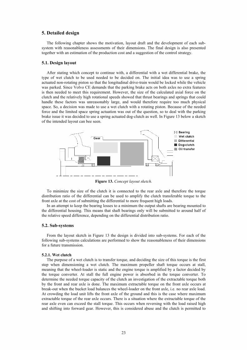
After stating which concept to continue with, a differential with a wet differential brake, the
type of wet clutch to be used needed to be decided on. The initial idea was to use a spring actuated non-rotating piston so that the longitudinal drive-train would be locked while the vehicle was parked. Since Volvo CE demands that the parking brake acts on both axles no extra features is then needed to meet this requirement. However, the size of the calculated axial force on the clutch and the relatively high rotational speeds showed that thrust bearings and springs that could handle these factors was unreasonably large, and would therefore require too much physical space. So, a decision was made to use a wet clutch with a rotating piston. Because of the needed force and the limited space spring actuation was out of the question, so to deal with the parking brake issue it was decided to use a spring actuated dog-clutch as well. In Figure 13 below a sketch of the intended layout can bee seen.
Figure 13. Concept layout sketch.
To minimize the size of the clutch it is connected to the rear axle and therefore the torque
distribution ratio of the differential can be used to amplify the clutch transferable torque to the front axle at the cost of submitting the differential to more frequent high loads.
In an attempt to keep the bearing losses to a minimum the output shafts are bearing mounted to the differential housing. This means that shaft bearings only will be submitted to around half of the relative speed difference, depending on the differential distribution ratio. 5.2. Sub-systems
From the layout sketch in Figure 13 the design is divided into sub-systems. For each of the
following sub-systems calculations are performed to show the reasonableness of their dimensions for a future transmission. 5.2.1. Wet clutch
The purpose of a wet clutch is to transfer torque, and deciding the size of this torque is the first step when dimensioning a wet clutch. The maximum propeller shaft torque occurs at stall, meaning that the wheel-loader is static and the engine torque is amplified by a factor decided by the torque converter. At stall the full engine power is absorbed in the torque converter. To determine the needed torque capacity of the clutch an investigation of the extractable torque both by the front and rear axle is done. The maximum extractable torque on the front axle occurs at break-out when the bucket load balances the wheel-loader on the front axle, i.e. no rear axle load. At crowding the load unit lifts the front axle of the ground and this is the case where maximum extractable torque of the rear axle occurs. There is a situation where the extractable torque of the rear axle even can exceed the stall torque. This occurs when reversing with the load raised high and shifting into forward gear. However, this is considered abuse and the clutch is permitted to
24
slip in such a situation. The propeller shaft torque, Mps max, for break-out and crowding can then be calculated by
axle
tiregNps N
RFM
⋅⋅=
μmaxmax , (18)
where FN max is the maximum axle load, μg is the tire to ground coefficient of friction, Rtire is the tire rolling radius and Naxle is the axle gear ratio. Numerical values for this calculation based on the L220 model can be seen in Table 3.
Table 3. Results extractable torque L220. Parameter Notation Front axle Rear axle Unit Max axle load FN max 505 229 [kN] Coefficient of friction μg 1 1 [-] Axle gear ratio Naxle 23,33 23,33 [-] Tire rolling radius Rtire 0,9 0,9 [m] Max extractable torque Mps max 19,5 8,8 [kNm] Stall torque Mstall 12,8 12,8 [kNm]
As seen in Table 3 the stall torque easily can be extracted on the front axle while the rear axle
in this case only can make use of about 70% of the stall torque. Since a differential with uneven torque distribution was chosen and the clutch is mounted on the rear output shaft the clutch will not have to handle the full stall torque. The maximum clutch torque for the break out case, Mcbo, can be calculated by
rM
M stallcbo = , (19)
where r is the differential distribution ratio. With r=1,5 the clutch toque can be calculated to 8,5 kNm which means that the crowding case will be dimensioning.
Designing a wet clutch is always a compromise between torque capacity, surface pressure, piston force, space requirements etc. In this case the inner and outer diameter of the friction discs was put as large as possible and thereby maximizing torque capacity and space utilization. The maximum axial force, Fc, on the clutch can then be expressed by
ffc
cc Rn
MF⋅⋅
=μ
, (20)
where Mc is the clutch torque capacity, µc is the coefficient of friction, nf is the number of friction interfaces and Rf is the friction radius which can be derived[1] by integration and calculated by
( )( )22
33
32
fifo
fifof RR
RRR
−⋅
−⋅= . (21)
The maximum surface pressure, pfd, is then
( )22fifo
cfd RR
Fp
−⋅=π
, (22)
where Rfo is the outer and Rfi is the inner radius of the friction surface. To determine the oil pressure, poil, needed to apply the clutch force one has to consider the maximum return spring force, Fs max, as well so
25
( )22max
pipo
scoil RR
FFp
−⋅+
=π
, (23)
where Rpo is the outer piston radius and Rpi is the inner. To determine the size of the needed spring force one must first investigate the rotation induced forces on the piston. The rotation induced force, Frot, can be calculated by[1]
( ) ( )[ ]222442
24 pipooilpiporot RRRRRF −⋅⋅−−⋅⋅⋅
=ωρπ
, (24)
where ω is the rotational velocity, ρ is the oil density and Roil is the oil level radius. Since the design requires a stand-by pressure, psb, to disengage the dog-clutch when the system is pressurized this will give an extra addition to the spring force, Fsp, needed to avoid self engagement of the clutch at high rotational speeds. This force can be calculated by
( )22piposbrotsp RRpFF −⋅⋅+= ∑ π , (25)
and the maximum spring force, Fsp max, that will effect the maximum oil pressure will then be
stspspsp LnkFF ⋅⋅+=max , (26)
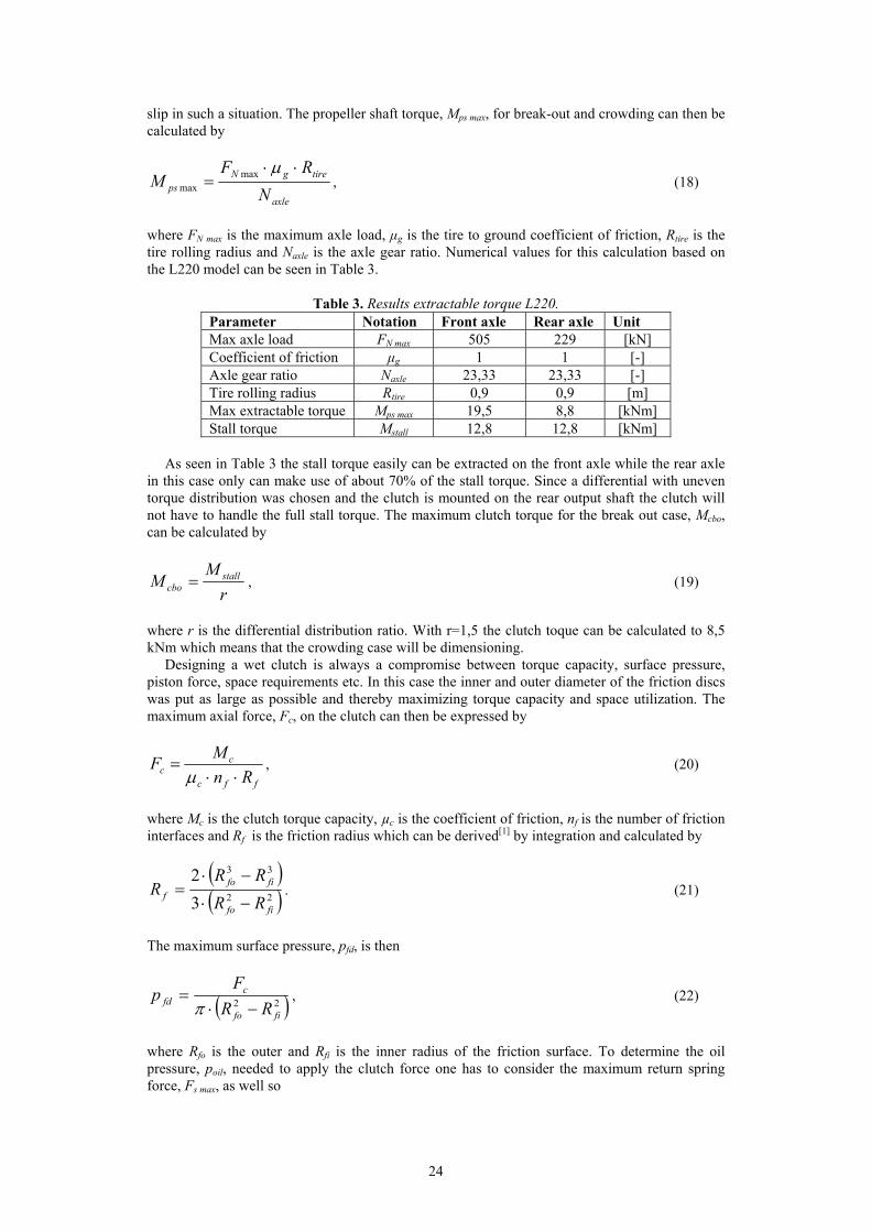
where k is the spring constant, nsp is the number of springs and Lst is maximum piston stroke length. The chosen clutch data for each parameter in the above equations can be seen in Table 4.
Table 4. Clutch data. Parameter Notation Size Unit Outer radius friction surface Rfo 119 [mm] Inner radius friction surface Rfi 100 [mm] Outer radius piston Rpo 115 [mm] Inner radius piston Rpi 75 [mm] Outer radius balance piston Rbp o 110 [mm] Inner radius balance piston Rbp i 75 [mm] Oil level radius piston Roil p 55 [mm] Oil level radius balance piston Roil bp 40 [mm] Number of friction interfaces nf 20 [-] Coefficient of friction μc 0,1 [-] Torque capacity Mc 9 [kNm] Max rotational speed ω 2600 [rpm] Oil density ρ 850 [kg/m3] Spring constant k 4,52 [N/mm] Number of springs nsp 25 [-] Max piston stroke length Lst 5 [mm]
With the numerical values in Table 4 the results presented in Table 5 can be calculated.
Table 5. Clutch calculation results. Variable Notation Size Unit Axial clutch force Fc 41 [kN] Friction disc surface pressure pfd 3,1 [MPa] Spring force disengaged Fsp 3,8 [kN] Max spring force engaged Fsp max 5,5 [kN] Max oil pressure poil 1,9 [MPa]

26
To get an estimation of the clutch power capacity an approximated heat accumulation ability in the separator discs are calculated according to
TmcQ Δ⋅⋅=Δ , (27) where c is the specific heat capacity, m is the total mass of the separator disc between the friction surfaces and ΔT is the change in temperature. If a 60°C temperature increase is allowed the absorbed heat would be about 78 kJ which can be compared to the energy of one wheel spinning with 170 rpm or the full engine power during 0.3 seconds. Both these cases are extreme and will most probably never have to be accommodated in the clutch. 5.2.2. Differential
The differential used in the concept is a two step planetary differential whit an uneven torque distribution ratio. This type of differential is axially compact and the torque distribution makes the use of a smaller clutch package possible.
For the differential, the worst load case is when the stall torque is transferred to the front shaft. In that case all torque is transferred via the differential gears. The differential gears are dimensioned from this static load case, which is considered enough since the loads on the gears are lower when they are rotating since the drive-train will be locked in low gears and the rotating speed of the gears are low even for an unlocked drive-train.
The final distribution ratio and the sizes of the differential gears were determined, and Mats Åkerblom at Volvo CE chose the gear geometry and performed gear strength calculations using Volvo’s calculation software. The final distribution ratio of the differential is 59/41, 59% of the torque to the front axle and 41% to the rear. The results of the calculations can be seen in Appendix F.
5.2.3. Dog-clutch
The dog-clutch is needed as a connection between the front and rear axle in conditions where the system oil pressure is zero, such as during parking or when utilizing the parking brake as an emergency brake. The requirements that limits both these cases are, for the L220, as follows
1. The parking brake shall hold the vehicle stationary with a weight of 40500 kg and 25%
slope. This assumes a rolling resistance of 0, the brake pressure is 0 MPa and a maximum tire rolling radius of 920 mm.
2. When using the parking brake as an emergency brake, the braking distance shall be maximum 26 m when braking from 32 km/h to 0 km/h with a machine weight of 40500 kg. (ISO 3450). The brake distance starts from the point where the brake pressure is 0 MPa and assumes a maximum tire rolling radius of 920 mm and a flat, dry tarmac surface.
From the above requirements the strain on the dog-clutch in both cases can be derived.
Case 1 – Stationary vehicle The brake force, Fbr, needed to hold the vehicle stationary can be written as
( )ϕsin⋅⋅= gmFbr , (28)
where m is the vehicle mass, g is the gravity constant and φ is the slope angle. The rear shaft moment, Mrs, for this force will then be
axle
tirebrrs N
RFM ⋅= , (29)
where Rtire is the maximum rolling radius and Naxle is the gear ratio of the axle.
Since the moment on the rear shaft has its reacting moment in the parking brake on the front shaft the moment is taken trough the differential and therefore the properties of the differential

27
has to be considered. A free body diagram of the shafts, the differential gears and the dog-clutch can be seen in Figure 14.
1. Rear companion flange
2. Rear differential gear
3. Dog-clutch
4. Front differential gear
5. Front companion flange
M1 M2 M3 M4 M5
1
2 34
5
Figure 14. Free body diagram.
From Figure 14 it is understood that M1 represents the rear shaft moment, Mrs, and M3 represents the dog-clutch moment, Mdc, so
1MM rs = (30) and
1MM dc = (31) M5 represents the parking brake moment and, since M1 and M5 are the only moments acting from the surroundings on the system, static equilibrium gives,
051 =+ MM . (32) Static equilibrium for each shaft gives
0321 =++ MMM (33) and
054 =+ MM . (34) The proportion of moment between the differential gears, M2 and M4, is governed by the ratio in the differential, r.
24 MrM ⋅= (35) To find the relation between the rear shaft moment, Mrs, and the moment acting on the dog-clutch, Mdc, equation (30), (31), (32), (33), (34) and (35) is used.
28
⎟⎠⎞
⎜⎝⎛ +⋅=
rMM rsdc
11 (36)
Case 2 – Emergency brake
If uniform acceleration is assumed the needed acceleration can be calculated by
svva
2
20
2 −= , (37)
where v0 is the initial speed, v is the end speed and s is the braking distance. The brake force, Fbr, needed to stop the vehicle within the prescribed distance can then be written as
amFbr ⋅= . (38)
The rear shaft moment can then be calculated using equation (29), and from that the dog-clutch moment can be calculated using equation (36). With numerical values one can see that the static case exert the larger moment on the dog-clutch and will therefore be dimensioning. In Appendix H these numerical values can be found together with an assessment of the reasonableness of surface pressure and shear stress levels in an approximated geometry for the dog teeth.
5.2.4. Bearings
All bearings used in the concept are calculated to make sure that the right choice of bearing has been done and that the bearing will stand the loads. There are two different bearing loads to consider, there is the static bearing load that only ensures that the bearing will stand its worst load case, and there is the dynamic bearing load witch gives the life of the bearing for the load collectives. The bearing calculations are performed on SKF bearings using their own methods[5].
For the shaft bearings, mounted to the front respective the rear shaft and the differential housing, only the static load case has to be considered since the rotational speeds of these bearings are low at all times. As dimensioning load for these bearings the load that emerges on the bearings from the axial force in the propeller shaft that appear due to the friction in the spline when it is sliding is used. This force acts mostly as an axial load on the bearing, why tapered roller bearings are used.
The needle bearings for the planetary gears in the differential are also only dimensioned from the static load case, also here since the rotational speeds are low. For these bearings the worst load case is when the forces on the gear flanks are at its top level which is when the stall torque is taken out on the front axle and all torque goes through the differential.
The only bearings in this concept that rotates continuously at high speeds are the housing bearings, mounted to the transmission housing and the differential housing; therefore these bearings have to be calculated both for the static load case. To ensure that the bearings will stand the static load the static load case is calculated and the dynamic load case is calculated to estimate the life of the bearings. For the static load case the dimensioning load is the force from the friction in the propeller shaft splines plus the forces that emerge from the drop gear[7] in the transmission. The dynamic load is calculated from a load collective containing different loads, at witch rotational speed they occur and their time fraction of the total operating time of the wheel loader. An example of such a load collective can be seen in Figure 15. For every load in the collective the life is calculated, and the life and time fraction is then taken into account when calculating the total life of the wheel-loader.
The conclusions that can be drawn from the calculations are that all chosen bearings will stand their highest static load and that the life of the housing bearings well exceeds the demands.
To see all calculations and the results for each bearing, see Appendix D.

29
Figure 15. Load collective, front axle pinion.
5.2.5. Hydraulic system
As a consequence of the decision to use a single oil channel for both the wet clutch cylinder and the dog-clutch cylinder the hydraulic system has to be more complicated. To disengage the dog-clutch during normal operations a stand-by pressure is needed. This is achieved by the use of a extra three port solenoid operated directional valve, a pressure control valve and a check valve as can be seen in the schematics in Figure 16.
Figure 16. Proposed layout of hydraulic system.
During normal operations the solenoid in directional valve will be powered and thereby supply
the cylinders with the stand-by pressure through the pressure control valve. The proportional valve then controls the pressure during engagement of the wet clutch. Should an emergency occur

30
the power to the directional valve will be turned off and thereby connecting the cylinders to the reservoir and locking the dog-clutch.
The needed flow rate was estimated to ~15 l/min for the maximum stroke length of the piston and an engagement time of 0.5 seconds which means that an accumulator would probably not be needed depending on the supply unit.
5.3. Final design
The basic features of the final design proposal are illustrated in the section view seen in Figure
17. All numbers within () in the following section refers to the numbers in Figure 17.
Figure 17. Section view of the final design proposal.
In the final design the oil transfer (1) had to switch place with the rear differential housing
bearing (2) compared to the design layout draft. This since the rear shaft bearings (3) had to be larger radial than first expected. The moving of the oil transfer resulted in a need for a new oil channel (4) in the transmission housing (10). To make that channel one drilling and two milling operations have to be added to the operations made when making transmission housing. These holes can be made in the multipurpose mill that is used to machine the transmission housing today, and in the same set up. The holes can be made in all produced housings whether they should have a differential or an ordinary longitudinal drive-train, since the holes do not affect the drive-train of today.
In order to save space the dog-clutch (5) and the wet-clutch (6) share the same oil channel (7), hence one oil transfer can be used instead of two which would be very space consuming. The control strategy is that at all times when the loader is running a small standby-pressure is keeping the spring (8) activated dog-clutch disengaged; this standby-pressure and the returns springs (18) of the wet-clutch piston (19) are chosen so that the wet-clutch is not activated at this pressure.

31
When activating the wet-clutch the pressure is increased, this does not affect the dog-clutch and it will still be disengaged. The spring activation of the dog-clutch means that it will only be engaged when the control pressure is under the standby level, due to failure or when the loader is turned off.
To make the oil transfer in the rear end of the transmission housing possible, the shimming of the differential housing bearings is moved to the front end of the transmission (9), this way a seal (20) can be placed between the transmission housing and the rear bearing housing (11) and the axial placement of the rotating seals will thereby have a shorter chain of tolerances.
The differential housing (12) has to be divided into three sections; one division is to make the mounting of the clutches possible and the other to make the mounting of the differential possible. The first division (13) is selected so that the screw joint that keeps the sections together will not have to transfer moment, only axial reaction force when the wet-clutch is engaged. It transfers moment from the dog-clutch, but that moment is small in the context and never occurs simultaneously with the axial force from the wet-clutch. The other division (14) is made so that the planetary carrier (15) is one section that is bolted to the housing after the differential gears (16) are mounted into it. The parts are connected with screw joints, calculations of these can be found in Appendix I. FEM-analysis of the differential housing and the pistons can be found in Appendix G.
Concerning the splines (17) connecting the rear solar gear and the clutch hub to the rear axle, this is done by only one spline on the shaft. The idea was, at first, to make the solar gear and the shaft in one piece and have only the clutch hub connected with a spline, but the limited axial space would have made it impossible to cut the spline so the solar gear had to be connected by a spline to. To see strength estimations of all splines in the concept, see Appendix H.
For the differential, the moment distribution ratio is 59/41, front/rear. This gives that the moment required in the wet-clutch for transferring stall torque to the front shaft is less than the 9000 Nm that the clutch is dimensioned for.
Drawings of all new parts included in the concept can be found in Appendix K.
5.4. Estimation of production cost
In order to estimate a production cost most of the parts in the concepts have been matched to part in other Volvo transmissions. Volvo’s buying prices for these parts have then been the basis of the estimation, Table 6. As a reference the prices of the parts from today’s solution, Table 7, have been put together in the same way to see the difference in price.
Table 6. Prices for the concept, SEK.
Part Price Shafts 2800 Wet-clutch 1700 Dog-clutch 200 Bearings 900 Oil transfer 1300 Outer housing parts 1400 Inner housing and drop gear 6000 Differential 2800 Sum 17100
Table 7. Prices for the current solution, SEK.
Part Price Shafts 1800 Bearings 300 Outer housing parts 1400 Drop gear 5000 Sum 8500

32
This comparison halts because many small parts are missing and the parking brake is excluded in the estimations. Furthermore the price of the parts in the concept will be dependent of the number of produced units. The assembling cost is excluded in the comparison, but will obviously be higher for the new concept than for today’s solution. The conclusion that can be made from these numbers is that the new concept will cost slightly more than twice the price of the current solution.
5.5. Suggestion of control strategy
The following suggestion of control strategy is our personal opinion based on the knowledge
acquired during this thesis work. In Figure 18 a diagram of the suggested control logic can be seen.
Gear
= 1 or 2
Velocity
Speed difference
> N %
Valve
Oil pressure
Clutch engage
Brake pressure
> X MPa
OR
Engagement time
Rotational speeds
Brake pressure
Figure 18. Simplified logic diagram of suggested control strategy.
The clutch engagement can be said to depend on three different conditions. First, the clutch
engagement should have a velocity dependency. In low vehicle velocities, where the main work with the machine takes place, the tractive effort is usually high and the benefits of a separated longitudinal drive-train are low it is favourable to keep the clutch engaged to avoid wheel slip. At higher velocities, i.e. transport, the tractive effort is low and the benefits of a separated drive-train are higher and therefore it is beneficial with a disengaged clutch. Instead of defining a certain velocity at which the clutch should engage/disengage we believe, based on our experience acquired during the test drive which can be seen in Appendix B, that a control strategy based on which gear is used suits better. Since the velocity intervals of the gears overlap the same velocity can be achieved on several gears but with a lower available torque on higher gears and thereby the risk of slip can be reduced.
The second condition for clutch engagement is used to avoid wheel slip at higher velocities. By monitoring the rotational speeds of both axles a limiting value of the speed difference can be used to detect wheel slip. The risk of wheel slip on third and fourth gear is considered very low and will probably only occur at very slippery conditions or with extremely low rear axle loads. A limiting value of the speed difference have not been set as it requires a larger knowledge and testing of the influence of tire type, tire pressure and axle load on the rolling circumference. The clutch disengagement in this case can be done by ramping down the pressure after a certain velocity dependent engagement time to detect if the slip condition is still fulfilled.
The third condition deals with the transfer of brake torque through the drive-train. Due to the separated drive-train the rear wheels will slip and the retardation ability of the vehicle will decrease if not the clutch is engaged during rapid retardations. During slow retardations however
33
clutch engagement is not necessary. A suitable control parameter for this could be the brake pressure. This is another parameter which requires more testing to determine the limits. One could discuss if not the speed difference condition would cover this case as well, however that would require a initial slip which could impair the retardation ability.

34
6. Conclusions and recommendations
After working with this project for a couple of months some conclusions have been made and some problems, that we recommend a deeper look into, have been spotted.
The first, obvious, conclusion is that the longitudinal drive-train can be separated, either by an axle disconnect or a differential with a locking device, and fitted in today’s transmission housing without having to make any radical changes to it. To get a detailed view of the concept see drawings in Appendix K.
With such a solution the parking brake could be changed from the wet brake inside the transmission of today to a dry disc brake placed on one of the propeller shafts, the coupling to the other propeller shaft could then be done by a spring activated dog-clutch. This is what our suggestion looks like today, and it is probably the easiest way to do it, but we believe that it could be beneficial to either place the parking brake on one shaft in the transmission, and thereby use the torque distribution in the differential to brake both axles, or have spring activation on the main brakes (like in trucks), and thereby make the parking brake totally independent of the drive-train. This would make the solution a lot less complicated since the need for a dog-clutch would vanish.
To determine if the differential concepts’ better handling performance, compared to the rear axle disconnect, compensate for its higher price testing of a prototype and dynamic simulations in slippery conditions would be favourable. Also, a deeper look into how expensive it would be to develop software for the axle disconnect that counterbalances its handling problems and makes it more competitive would be good before it is expelled. We are convinced that the stability problems of the axle disconnect can be dealt with since many car manufactures has done it with dazzling results.
The fuel savings due to a separated drive-train should be more thoroughly investigated. Our calculations are only based on one small test of fuel saving potential that is assumed to be valid for the whole wheel-loader fleet, the result shows a negligible fuel saving, Appendix A. This is mainly because many wheel-loaders are only used at low speeds where the separated drive-train does not contribute, tests and further researches where the focus is on wheel-loaders that is used mostly for load carrying would most likely show a higher fuel saving potential. It is for those wheel-loaders a separated drive-train would be most beneficial, the self oscillation also occur mostly for the load carrying wheel-loaders.
I order to assimilate the potential of the separated drive-train to reduce stresses in the axles the brake setup or controlling strategy must be remade in some way. By only separating the drive-train without changing the brake setup the result will be that the rear wheels will slip when braking, especially when braking downhill with load in the bucket. This behaviour is unpleasant, increases tire wear and braking distance, and can cause the driver to lose control of the vehicle. To reach the same braking distance as today the brake capacity of the brakes in the front axle will have to be increased, the brake capacity of the brakes in the rear axle might also have to be increased to ensure good retardation capacity when reversing; we have not looked into that so it is something that has to be done. The wheel slip has to be dealt with by some kind of control strategy; the easiest one would be to adjust the brake pressure so that the front axle gets higher pressure than the rear axle when driving forward and vice versa when reversing. This strategy could solve the problem with the wheel slip but would have to be calibrated for a worst case, fully loaded bucket, and therefore would not utilize the brake capacity to its max in other cases. Another, more refined, strategy would be to have a load sensing system that could set the brake pressure proportion between the front and rear axle depending on the axle pressure, that could be calculated from the load weight in the bucket. An even more refined strategy is to equip the loaders with ABS, Anti-lock Braking System; it would avoid wheel slip, utilize all available fiction for each tire and could give stability advantages when braking in slippery conditions. To find a good solution for the brakes a deeper investigation has to be done concerning only this matter to se what could be done and what is unrealistic. For our concept, since it contains a differential brake, one can lock the drive-train and the braking capacity will be exactly as it is today, but then the risk of seizure in the differential carrier gear set will still be present.

35
7. List of references Literature [1] M. Anleitner, Wet brake & Clutch Technology, Livonia Technical Services Co [2] D. Myhrman, Terängmaskinen Del 1, SkogForsk, 1993 [3] K-O. Olsson, Maskinelement, Liber AB, 9147052732, Stockholm, 2006-01 [4] B. Sundström, Handbok och formelsamling i hållfasthetslära, KTH, 1999 [5] SKF, Huvudkatalog 6000SV, 2006 [6] C. Nordling, J. Österman, Physics handbook for science and engineering, Lund, 2004 [7] E. Eriksson, O. Isaksson, E. Kassfeldt, S. Lagerkrans, E. Höglund, J. Lundberg, Maskinelement, Luleå, 1991 [8] O. Isaksson, Grundläggande hydraulik, Luleå, 1999 [9] K. Ulrich, S. Eppinger, Product Design And Development, Singapore, 2003 [10] Michelin Earthmover Department, Technical characteristics Michelin 29.5 R 25 XLD D2 A TL*, 1993. [11] Michelin Earthmover Department, Technical characteristics Michelin 23.5 R 25 XHA TL*, 2004. Internal documents [12] System Specification L220 drive train, Requirement agreement between HLD and CMP [13] Strandberg, J., Beräkning bromsar lastar 2628-modeller. (TeamPlace 76200 Driveline systems) Växellåda till dumper CAT D250E. Inspektion av växellåda. Rapport nr PRO98GDCK042748. Sörensson A., Test report draft, Fuel consumption with and without rear shaft, 2009. Strandberg L. Reg nr SR01LS0032, Körfallskatalog - Lasta/bär i backe, 2001. Strandberg L. Reg nr SR01LS0032, Körfallskatalog - Lasta/bär i plan mark, 2001. Strandberg L. Reg nr SR01LS0032, Körfallskatalog - Kort lastarcykel, 2001. Oral references Joakim Lundin, Design Engineer – Wet clutches, R&D Driveline Design, Volvo CE, Eskilstuna Ralf Nordström, Lead Engineer – Axle Technology, Driveline Technology, Volvo CE, Eskilstuna Mats Åkerblom, Design Engineer, R&D Driveline Design, Volvo CE, Eskilstuna Thomas Andersson, Design Engineer – Bevel gears, R&D Driveline Design, Volvo CE, Eskilstuna Johnny Strandberg, Design Engineer – Brakes, R&D Driveline Design, Volvo CE, Eskilstuna Henrik Strand, Bearing Expert, Structures and Durability Europe, Volvo CE, Eskilstuna Tore Oscarsson, Engineering, Loader Platform, Volvo CE, Eskilstuna Andreas Nordstrand, Design Engineer, Emerging Technologies, Volvo CE, Eskilstuna Fredrik Rydholm, Product Planner, Component & Technology Planning, Volvo CE, Eskilstuna Daniel Jansson, Design Engineer - Transmissions, Driveline Technology, Volvo CE, Eskilstuna Johan Aleberg, Design Engineer – Hydraulics, R&D Driveline Design, Volvo CE, Eskilstuna Images [I] John Deere product and information training bulletin, No. 08WL16 [II] http://en.wikipedia.org/wiki/File:Differential_free.png, Author: Wapcaplet

Appendix A - Fuel saving potential. Page: 1(2)
This document contains calculations of the fuel savings that can be made by separating the longitudinal drive-train in the L220F. The calculations are made based on the fuel consumption measured in the L220F with and without rear shaft and the distribution of speeds for the whole L220F fleet. Input The measured fuel consumption from the test, Fuel consumption with and without rear shaft – A. Sörensson, can be seen in Table 1.
Table 1. Measured fuel consumption. Case l/h normal l/h no rear shaft Volume difference % 31 km/h gravel 28,25 27,95 -2,1 17 km/h gravel 15,18 14,61 -3,7 31 km/h asphalt 25,2 24,88 -0,1 41 km/h asphalt 44,28 43,05 -3,5 17 km/h gravel loaded 16,58 16,22 -1,0
The speed distribution for the fleet collected from Analys Matris for L220F can be seen in Table 2.
Table 2. Time spent within speed interval. Speed km/h
0-<0,5
0,5-<4,5
4,5-<9
9-<13,5
13,5-<18
18-<22,5
22,5-<27
27-<31,5
31,5-<36
36-<40,5
40,5-
% time
37,1 22,1 22,8 10,1 4,1 2,3 1,0 0,3 0,1 0,1 0,0
The mean fuel consumption for the fleet can be collected from Analys Matris and is 19,7 l/h. The mean idling fuel consumption for the fleet can be collected from Analys Matris and is 4,6 l/h. Assumptions The assumptions for the following calculations are
1. The fuel consumption for speeds under 13,5 km/h is the same for both drive-train constellations. This is assumed since the separated drive-train probably will be locked in the first two gears.
2. The fuel consumption for 13,5-22,5 km/h is approximately the mean consumption for the two test runs in 17 km/h.
3. The fuel consumption for 22,5-36km/h is approximately the mean consumption for the two test runs in 31 km/h.
4. The fuel consumption for speeds over 36km/h is approximately the consumption for the test run in 41 km/h.
5. In the speed interval 0-0,5 km/h all idling is included therefore an assumption is made that only 50% of the time in this interval is actual driving.

Appendix A - Fuel saving potential. Page: 2(2)
Calculations For the original drive-train layout the fuel consumption for speeds under 13,5 km/h can be calculated from the mean consumption minus the consumptions for the higher speeds and idling, times their time share divided with its own time share. For the concept with separated drive-train overall consumption can be calculated from the fuel consumptions at each speed times its time share. This can bee seen in Table 3.
Table 3. Mean fuel consumption for speed intervals. Speed km/h Idling *0-<13,5 13,5-<22,5 22,5-<36 36- *0- 0- % time 18,5 73,6 6,4 1,4 0,1 81,5 100 Mean l/h normal
4,60 23,63 16,19 26,73 44,28 23,13 19,70
Mean l/h no rear shaft
4,60 23,63 15,42 26,42 43,05 23,06 19,65
*Idling excluded. This gives a fuel saving average of 0,25 % for the separated drive-train with idling included. With idling excluded the average fuel saving for the fleet is 0,30%. Conclusions and discussion The result with a fuel saving of 0,25% respective 0,30% seams reasonable but it is not an exact value since the assumptions are pretty rough and the fuel consumption for the higher speeds are based on a single test. From a simplified approximation with a fuel saving of 4 % for higher speeds that is approximately 10 % of the usage time one get a fuel saving of ~0,4 %. This shows that the separated drive-train will be hard to motivate as standard equipment but for customers that uses their wheel-loaders a lot for load-carrying applications, hence have a bigger part of the usage time at higher speeds, it could be an interesting option.

Appendix B - Separated drive-train - Driving dynamics test Page: 1(3)
The following pages presents a comparison of the vehicle handling and retardation capability of an L150F with four wheel drive, front wheel drive and rear wheel drive. The test is performed to investigate the benefits and drawbacks of a separated longitudal drive-train. The conclusions that could be made were that the retardation capability for the separated drive-train was severely reduced and the vehicle handling, in most senses, was also affected negatively.
Cases 1. Retardation Execution: Maximum brake from >20 km/h on gravel and asphalt. Purpose: Investigate stability, retardation and wheel lock-up. 2. Turning radius Execution: Driving with full steering and measuring the turning radius. Purpose: Investigate tendencies for over- and under-steering. 3. Sharp curves Execution: Cornering in connected curves at speeds >10 km/h. Purpose: Investigate stability and skid tendency. 4. Ascent Execution: Start in a steep slope and driving in a shallow slope in 10 km/h. Purpose: Investigate traction. 5. Descent Execution: Controlled descent using brakes or engine brake. Purpose: Investigate stability and retardation. 6. Snaking Execution: Driving with varying throttle level and speeds. Purpose: Investigate snaking tendency. 7. Oscillation Execution: Driving with varying throttle level and speeds perhaps use a bump to trigger the oscillation. Purpose: Investigate self-oscillation properties.
Table 1. Test compilation. Test Case Loaded*/Empty Surface Comments 1.1 Retardation Empty Gravel 1.2 Retardation Empty Asphalt 1.3 Retardation Loaded Gravel 1.4 Retardation Loaded Asphalt 2.1 Turning radius Empty Gravel 2.2 Turning radius Loaded Gravel 3.1 Sharp curves Empty Gravel 3.2 Sharp curves Loaded Gravel 4.1 Ascent Empty Gravel 4.2 Ascent Loaded Gravel 5.1 Descent Empty Gravel Brakes 5.2 Descent Empty Gravel Engine brake 5.3 Descent Loaded Gravel Brakes 5.4 Descent Loaded Gravel Engine brake 6.1 Snaking Empty/Loaded Gravel/Asphalt 7.1 Oscillation Empty/Loaded Gravel/Asphalt
*Load 6,7 ton ~ full 4m3 bucket
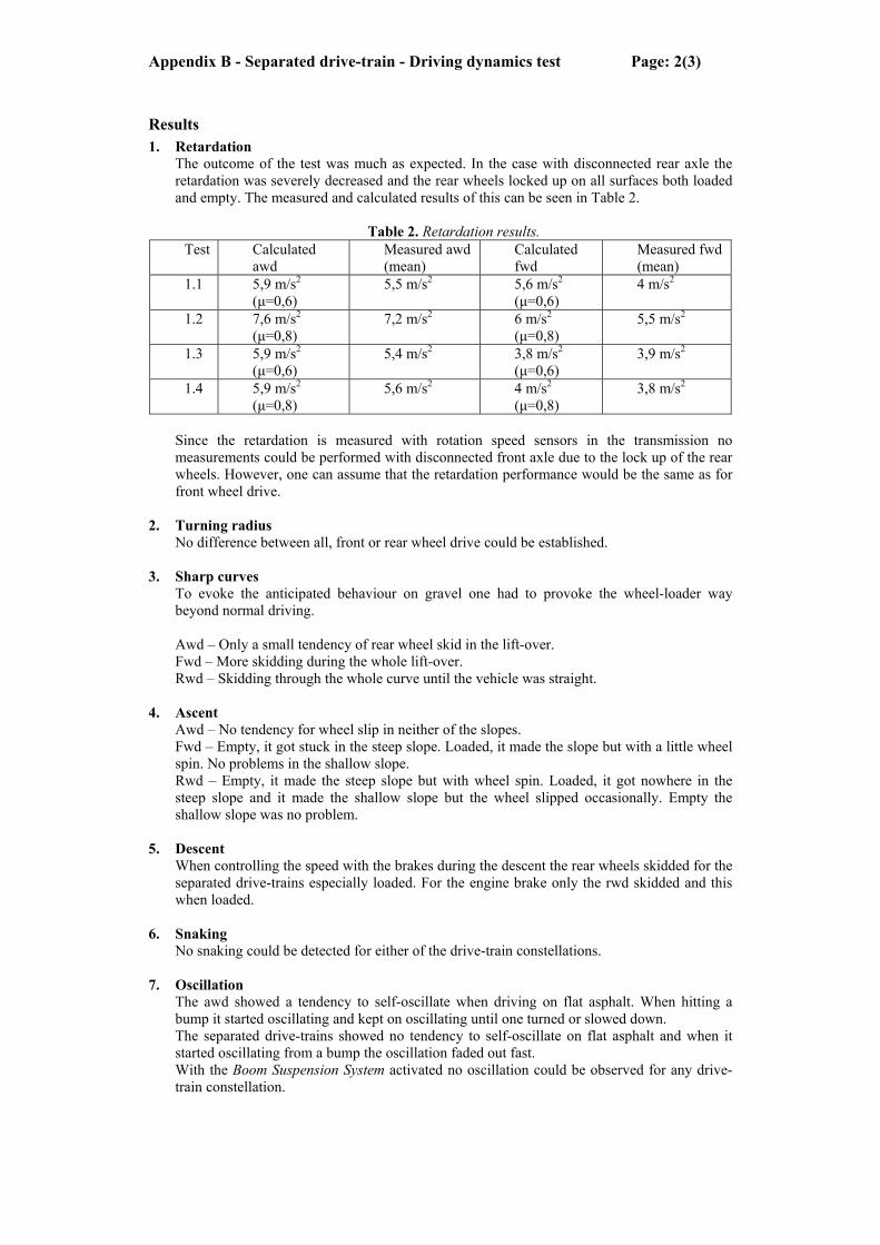
Appendix B - Separated drive-train - Driving dynamics test Page: 2(3)
Results 1. Retardation
The outcome of the test was much as expected. In the case with disconnected rear axle the retardation was severely decreased and the rear wheels locked up on all surfaces both loaded and empty. The measured and calculated results of this can be seen in Table 2.
Table 2. Retardation results. Test Calculated
awd Measured awd (mean)
Calculated fwd
Measured fwd (mean)
1.1 5,9 m/s2 (μ=0,6)
5,5 m/s2 5,6 m/s2 (μ=0,6)
4 m/s2
1.2 7,6 m/s2 (μ=0,8)
7,2 m/s2 6 m/s2 (μ=0,8)
5,5 m/s2
1.3 5,9 m/s2 (μ=0,6)
5,4 m/s2 3,8 m/s2 (μ=0,6)
3,9 m/s2
1.4 5,9 m/s2 (μ=0,8)
5,6 m/s2 4 m/s2 (μ=0,8)
3,8 m/s2
Since the retardation is measured with rotation speed sensors in the transmission no measurements could be performed with disconnected front axle due to the lock up of the rear wheels. However, one can assume that the retardation performance would be the same as for front wheel drive.
2. Turning radius No difference between all, front or rear wheel drive could be established.
3. Sharp curves To evoke the anticipated behaviour on gravel one had to provoke the wheel-loader way beyond normal driving. Awd – Only a small tendency of rear wheel skid in the lift-over. Fwd – More skidding during the whole lift-over. Rwd – Skidding through the whole curve until the vehicle was straight.
4. Ascent Awd – No tendency for wheel slip in neither of the slopes. Fwd – Empty, it got stuck in the steep slope. Loaded, it made the slope but with a little wheel spin. No problems in the shallow slope. Rwd – Empty, it made the steep slope but with wheel spin. Loaded, it got nowhere in the steep slope and it made the shallow slope but the wheel slipped occasionally. Empty the shallow slope was no problem.
5. Descent When controlling the speed with the brakes during the descent the rear wheels skidded for the separated drive-trains especially loaded. For the engine brake only the rwd skidded and this when loaded.
6. Snaking No snaking could be detected for either of the drive-train constellations.
7. Oscillation The awd showed a tendency to self-oscillate when driving on flat asphalt. When hitting a bump it started oscillating and kept on oscillating until one turned or slowed down. The separated drive-trains showed no tendency to self-oscillate on flat asphalt and when it started oscillating from a bump the oscillation faded out fast. With the Boom Suspension System activated no oscillation could be observed for any drive-train constellation.
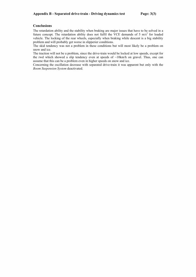
Appendix B - Separated drive-train - Driving dynamics test Page: 3(3)
Conclusions The retardation ability and the stability when braking are major issues that have to be solved in a future concept. The retardation ability does not fulfil the VCE demands of 5 m/s2 for loaded vehicle. The locking of the rear wheels, especially when braking while descent is a big stability problem and will probably get worse in slipperier conditions. The skid tendency was not a problem in these conditions but will most likely be a problem on snow and ice. The traction will not be a problem, since the drive-train would be locked at low speeds, except for the rwd which showed a slip tendency even at speeds of ~10km/h on gravel. Thus, one can assume that this can be a problem even in higher speeds on snow and ice. Concerning the oscillation decrease with separated drive-train it was apparent but only with the Boom Suspension System deactivated.

Appendix C - Concept evaluation. Page: 1(2)
The criterions used to evaluate the concepts in the Pugh matrix, seen in Figure 1, were chosen together with Volvo engineers. In this document an explanation of each criteria and the result of the evaluation can be seen.
Evaluation criteria
Ease of control Refers to the complexity of designing a completely autonomous control system that can compensate for the concepts weaknesses so that performance, compared to the original solution, is not compromised. Ability to transfer brake torque How well the concept can transfer brake torque from the rear brakes through the drive-train to the front wheels. Ability to reduce torque transfer between axles How well the concept can reduce unwanted wind-up torques in the drive-train. Driving stability How the vehicle handling is affected by the concept. Required space The physical space consumed by the designed concept. Production cost The cost of serial production compared to today’s solution. Lifecycle cost TCO, Total Cost of Ownership, refers to how much potential savings for the customer each concept provides. Reliability How the reliability of the wheel-loader is affected by each concept. Development cost Internal costs for the development of a product for serial production. Noise level How the noise of the machine is affected, gear noise etc. Efficiency How is the vehicle efficiency affected by the different concepts? Durability How durable is the concepts? Serviceability Is the complexity of service affected? Do the concepts affect the service interval? Volvo business case Money making potential for Volvo.

Appendix C - Concept evaluation. Page: 2(2)
Figure 1. Pugh's matrix.

Appendix D - Bearing dimensioning Page: 1(6)
This document contains calculations for the dimensioning of included bearings. To make sure that the bearings can stand the maximal load they can be exposed to, static load calculations are done for all bearings. The life of the housing bearings is also calculated to see how long they will bear.
Shaft bearings The shaft bearings connect the shafts to the differential housing; they only rotate with the speed difference between the housing and the shafts which can be considered low. Forces acting on the bearings are mainly the forces that result from the axial forces in the propeller shafts. These forces occur due to the friction in the propeller shaft splines. Since the speeds are low the bearings can be dimensioned from a static load case where safety factor, s0, is solved by
0
00 P
Cs = , (1)
where C0 is the static load rating for the bearing and P0 is the equivalent static bearing load. P0 is determent by the radial force, Fr, and the axial force, Fa, acting on the bearing
ar FYFP ⋅+⋅= 00 5,0 , (2) where Y0 is the static axial factor for the bearing. The forces, Fr and Fa, acting on the bearing are components of the axial force from the propeller shaft, Fp, dependent of the angle of the propeller shaft, αp, in respect to the shaft mounted by the bearing. Thus the forces can be described by
)sin( ppr FF α⋅= (3)
and
)cos( ppa FF α⋅= . (4)
(3) and (4) in (2) gives
))cos()sin(5,0( 00 ppp YFP αα ⋅+⋅= (5)
The frictional force in the propeller shaft, Fp, can be estimated by
rM
Fs
pp ⋅
⋅=
)cos(αμ
(6)
where μ is the coefficient of friction in the spline, Mp is the propeller shaft moment, αs is the nominal pressure angle of the spline and r is the mean radius for the spline. In Table 1 the used input data can be found.
Table 1. Input data shaft bearings static Variable Rear Front Bering nr. SKF 32010 X/Q SKF 32014 X/Q
C0 127 kN 153 kN

Appendix D - Bearing dimensioning Page: 2(6)
Y0 0,7 0,8 Mp max 9000 N 12800 N μ 0,3 0,3 αs 30° 30° r 45 mm 45 mm αp 10° *20°
*For the front propeller shaft the angle can vary from approximately -20 to 20 degrees, in this interval P0 has its highest value at 20 and -20 degrees. Table 2 shows the result of the calculations.
Table 2. Output data shaft bearings static Variable Rear Front
Fp 69 kN 99 kN P0 54 kN 91 kN s0 2,36 1,68
These safety factors are satisfying, especially since this load case does not occur very often, and the coefficient of friction is set to a value much higher than it is likely to be.
Housing bearings The housing bearing mounts the differential housing to the transmission housing.
Static The housing bearings will, for the static load case, have to manage both the resulting forces from the axial force in the propeller shaft and the resulting forces from the drop gear. For the drop gear the following equations can be defined.
)sin( bnax FF β⋅= (7) Where Fax is the axial resultant of the normal force, Fn, acting on the gear flank and βb is the base helix angle of the gear.
)sin()cos( tbnrad FF αβ ⋅⋅= (8) Where Frad is the radial resultant of the normal force of the gear flank and αt is the transposed normal pressure angle, which is calculated from the normal pressure angle, α, and the helix angle, β, as
⎟⎟⎠
⎞⎜⎜⎝
⎛=
)cos()tan(arctan
βαα t . (9)
The peripheral resultant, Fper, of the normal force of the gear is calculated by
)cos()cos( tbnper FF αβ ⋅⋅=. (10)
This peripheral resultant, Fper, is the torque transferring force acting on the gear and the following expression can be defined,

Appendix D - Bearing dimensioning Page: 3(6)
d
dper R
MF = , (11)
where Md is the moment of the drop gear and Rd is its radius. The axial force acting on the bearing, Fab, is calculated from the axial force from the propeller shaft, Fa, equation (4) and (6) and the axial force from the drop gear, Fax, equation (7), (10) and (11),
⎟⎟⎟⎟⎟
⎠
⎞
⎜⎜⎜⎜⎜
⎝
⎛
⎟⎟⎠
⎞⎜⎜⎝
⎛⋅
⋅+⋅
⋅
⋅=
)cos()tan(cos(arctan
)tan()cos(
)cos(βα
βα
αμ
d
bdp
s
pab
R
Mr
MF (12)
The radial force acting on the bearing, Frb, is the forces Fper and Frad, equation (8), (9), (10) and (11), added and since they are perpendicular this is done as
2
)cos()tan(1 ⎟⎟⎠
⎞⎜⎜⎝
⎛+⋅⋅=
βα
d
dfrb R
MdF (13)
where df is the radial force distribution factor depending on how close the bearing is to the gear. For this case the equivalent static load, P0, is calculated by
abrb FYFP ⋅+⋅= 00 5,0 (14) The safety factor is calculated by equation (1). In Table 3 the used input data can be found.
Table 3. Static input data, housing bearings. Variable Front Rear Bering nr. SKF 32924 SKF 32922 X/Q
C0 305 kN 224 kN Y0 0,9 0,9
Mp max 9000 N 12800 N Md max 12800 N 12800 N μ 0,3 0,3 αs 30° 30° r 45 mm 45 mm αp 10° *20° β 20° 20° βb 18°44´50´´ 18°44´50´´ α 20° 20° df 0,28 0,72 Rd 148 mm 148 mm
Table 4 shows the result of the calculations.
Table 4. Static output data, housing bearings. Variable Front Rear
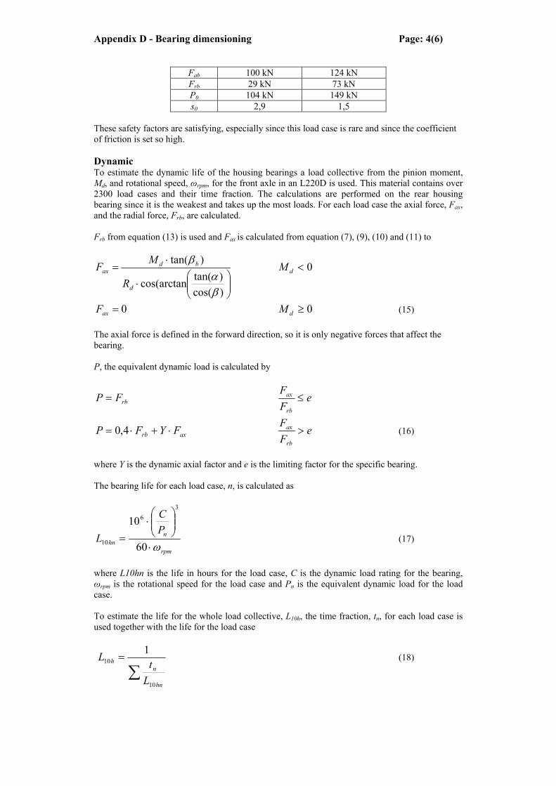
Appendix D - Bearing dimensioning Page: 4(6)
Fab 100 kN 124 kN Frb 29 kN 73 kN P0 104 kN 149 kN s0 2,9 1,5
These safety factors are satisfying, especially since this load case is rare and since the coefficient of friction is set so high. Dynamic To estimate the dynamic life of the housing bearings a load collective from the pinion moment, Md, and rotational speed, ωrpm, for the front axle in an L220D is used. This material contains over 2300 load cases and their time fraction. The calculations are performed on the rear housing bearing since it is the weakest and takes up the most loads. For each load case the axial force, Fax, and the radial force, Frb, are calculated. Frb from equation (13) is used and Fax is calculated from equation (7), (9), (10) and (11) to
⎟⎟⎠
⎞⎜⎜⎝
⎛⋅
⋅=
)cos()tan(cos(arctan
)tan(
βα
β
d
bdax
R
MF 0<dM
0=axF 0≥dM (15) The axial force is defined in the forward direction, so it is only negative forces that affect the bearing. P, the equivalent dynamic load is calculated by
rbFP = eFF
rb
ax ≤
axrb FYFP ⋅+⋅= 4,0 eFF
rb
ax > (16)
where Y is the dynamic axial factor and e is the limiting factor for the specific bearing. The bearing life for each load case, n, is calculated as
rpm
nhn
PC
Lω⋅
⎟⎟⎠
⎞⎜⎜⎝
⎛⋅
=60
103
6
10 (17)
where L10hn is the life in hours for the load case, C is the dynamic load rating for the bearing, ωrpm is the rotational speed for the load case and Pn is the equivalent dynamic load for the load case. To estimate the life for the whole load collective, L10h, the time fraction, tn, for each load case is used together with the life for the load case
∑=
hn
nh
Lt
L
10
101
(18)

Appendix D - Bearing dimensioning Page: 5(6)
Since the load cases are only for the front axle the loads from the rear axle are missing, this can be corrected by doubling all moments for the load cases and calculate the life, L10h2, the same way as L10h was calculated. This estimation will be an understatement of the life since the loads on the rear axle rarely are as high as the ones on the front axle. The life will in fact be somewhere between L10h2 and L10h. In Table 5 the used input data can be found.
Table 5. Input data housing bearing dynamic Variable Rear Bering nr. SKF 32922 X/Q
C 125 kN Y 1,7 β 20° βb 18°44´50´´ α 20° df 0,72 Rd 148 mm
Table 6 shows the results of the calculations.
Table 6. Output data housing bearing dynamic Variable Rear
L10h 324 000 h L10h2 40 000 h
This shows that the bearings will have a long enough life.
Planetary gear bearings The planetary gear bearings are mounted to the planetary gears and their axles. All loads on these bearings acts radial on the bearings, why needle bearings can be used, the rotational speeds are low, so the bearings can be dimensioned from the static load case. As dimensioning load, the load that acts on the bearing when the stall torque is taken out on the front shaft is used. To calculate the forces acting on the gears in the differential the easiest way is to chose a direction and sum all forces in that direction together. In this case the direction from the contact between the solar gear and the planetary gear to the centre of the planetary gear, this direction is called y. all forces in the y-direction is summed to Fy
)sin()cos(Pr ββ ⋅+⋅+= PperadSrady FFFF , (19) where FSrad is the radial contact force to the solar gear, FPrad is the radial contact force between the planetary gears and FPper is the periphery contact force between the planetary gears, the angle between those two contacts is β in this equation. From the y-direction a perpendicular x-direction is defined, and all forces in this direction is summed to Fx
)sin()cos( Pr ββ ⋅+⋅−= adPperSperx FFFF , (20) where FSper is the periphery contact force to the sun gear. Since there are no axial forces acting on the gears, the equivalent static bearing load, P0, can be defined as
220 xy FFP += (21)

Appendix D - Bearing dimensioning Page: 6(6)
The safety factor for the bearings, s0, is calculated by equation (1). Table 7 contains all input variables for each planetary gear bearing.
Table 7. Input data, planetary gear bearings.
In Table 8 the results of the calculations can be seen.
Table 8. Output data, planetary gear bearings. P0 113 kN 102 kN s0 1,0 1,4
The safety factor for the rear planetary gear bearing is really near the limit. This could probably be okay since this load only occurs at stall torque in reverse, at stall torque in forward the safety factor is almost five. But the planetary gear could be switched to a bigger one allowing a bigger bearing and decreasing the angle β, witch would lead to a higher safety factor for the worst load case. The safety factor for the front planetary gear bearings is okay, the forces will never exceed those values and the load case is rare. Conclusions The calculations show that all bearings will stand their worst static load case with satisfying safety factors. For the rear planetary gear bearing load is really close to the bearings limit but that load case corresponds to the stall torque taken out on the front axle in reverse which is a load case that if not never so very seldom occurs. The exact life of the housing bearings is hard to determine but what can be concluded is that it will be long enough.
Rear planetary gear Front planetary gear Bearing SKF k 55x60x30 2x SKF k 30x40x30
C0 108 kN 2x 69,5 kN β 79° 58°
FSper 53,5 53,5 FSrad 28,5 27,5 FPper 52,5 52,5 FPrad 30 30

Appendix E - Dog-clutch dimensioning Page: 1(4)
The purpose of the dog-clutch is to lock the front and rear axle together when the system pressure is zero, i.e. when the parking brake is used either in static conditions or as an emergency brake. This document contains the derivation of the limiting load cases together with an assessment of approximated dimensions of the dog-clutch.
Requirements L220 • The parking brake shall hold the vehicle stationary with a weight of 40500 kg and 25%
slope. This assumes a rolling resistance of 0, the brake pressure is 0 MPa and a maximum tire rolling radius of 920 mm.
• When using the parking brake as an emergency brake, the braking distance shall be maximum 26 m when braking from 32 km/h to 0 km/h with a machine weight of 40500 kg. (ISO 3450). The brake distance starts from the point where the brake pressure is 0 MPa and assumes a maximum tire rolling radius of 920 mm and a flat, dry tarmac surface.
Case 1 – Stationary vehicle The brake force, Fb, needed to hold the vehicle stationary can be written as
( )ϕsin⋅⋅= gmFb , (1) where m is the vehicle mass, g is the gravity constant and φ is the slope angle. The rear shaft moment, Mrs, for this force will then be
axle
tirebrs N
RFM
⋅= , (2)
where Rtire is the maximum rolling radius and Naxle is the gear ratio of the axle. Since the moment on the rear shaft has its reacting momentum in the parking brake on the front shaft the momentum is taken trough the differential and therefore the properties of the differential has to be considered. A free body diagram of the shafts, the differential gears and the dog clutch can be seen in Figure 1.
1. Rear companion flange
2. Rear differential gear
3. Dog-clutch
4. Front differential gear
5. Front companion flange
M1 M2 M3 M4 M5
1
2 34
5
Figure 1. Free body diagram

Appendix E - Dog-clutch dimensioning Page: 2(4)
From Figure 1 it is understood that M1 represents the rear shaft moment, Mrs, and M3 represents the dog clutch momentum, Mdc, so
1MM rs = (3) and
1MM dc = (4) M5 represents the parking brake momentum and, since M1 and M5 are the only moments acting from the surroundings on the system, static equilibrium gives,
051 =+ MM . (5) Static equilibrium for each shaft gives
0321 =++ MMM (6) and
054 =+ MM . (7) The proportion of momentum between the differential gears, M2 and M4, is governed by the ratio in the differential, r.
24 MrM ⋅= (8) To find the relation between the rear shaft moment, Mrs, and the moment acting on the dog clutch, Mdc, equation (3), (4), (5), (6), (7) and (8) is used.
⎟⎠⎞
⎜⎝⎛ +⋅=
rMM rsdc
11 (9)
Case 2 – Emergency brake If uniform acceleration is assumed the needed acceleration can be calculated by
svva
2
20
2 −= , (10)
where v0 is the initial speed, v is the end speed and s is the braking distance. The brake force, Fb, needed to stop the vehicle within the prescribed distance can then be written as
amFb ⋅= . (11) The rear shaft moment can then be calculated using equation (2), and from that the dog clutch moment can be calculated using equation (9).

Appendix E - Dog-clutch dimensioning Page: 3(4)
Dog teeth The section area, As, of each tooth can be approximated as the difference between two circle sectors
( )22
21
ios RRA −⋅⋅= θ , (5)
where θ is the sector angle, Ro is the outer radius and Ri is the inner radius of the tooth. The force that act upon the tooth, Ft, can be approximated from the dog-clutch moment as
( )iot
dct RRn
MF
+⋅⋅
= max2, (6)
where nt is the number of teeth. From the tooth force and the section area the mean shear stress, τm, now can be calculated by
s
tm A
F=τ . (7)
The contact pressure, pt, between the teeth can calculated as
( )iot
tt RRd
Fp−⋅
= , (8)
where dt is the tooth depth.
Load calculations In Table 1 the input data for the Volvo L220 used can be found.
Table 1. Dog-clutch input data. Parameter Value Unit
m 40500 kg g 9,8 m/s2 φ 25% - Ri 50 mm Ro 40 mm
Rtire 920 mm dt 5 mm nt 8 -
Naxle 23,33 - θ 0,44 rad v 0 km/h v0 32 km/h s 26 m r 1,5 -
Table 2 shows the result of the calculations.
Table 2. Dog-clutch output data. Variable Stationary vehicle Emergency brake
a - -1,5 m/s2

Appendix E - Dog-clutch dimensioning Page: 4(4)
Fb 96,3 kN 61,5 kN Mdc 6,3 kNm 4,0 kNm τm 89 MPa 57 MPa pt 351 MPa 225 MPa
From the calculated values one can see that Case 1 exerts a larger moment on the dog-clutch and therefore this will be dimensioning. Conclusions The calculations show that the stress levels in the dog-clutch are reasonable even for its worst load case.
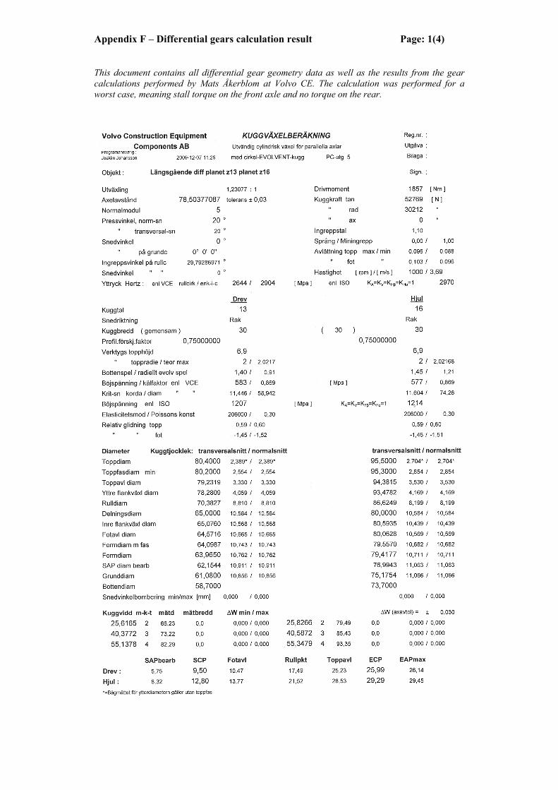
Appendix F – Differential gears calculation result Page: 1(4)
This document contains all differential gear geometry data as well as the results from the gear calculations performed by Mats Åkerblom at Volvo CE. The calculation was performed for a worst case, meaning stall torque on the front axle and no torque on the rear.

Appendix F – Differential gears calculation result Page: 2(4)

Appendix F – Differential gears calculation result Page: 3(4)

Appendix F – Differential gears calculation result Page: 4(4)
Conclusions Since Volvo lacks the experience of differential concepts in the longitudinal drive-train there
are currently no load collectives for dimensioning available, so dynamical calculations could not be performed. The calculations performed on the static load case show that the stress levels are high but acceptable according to Volvo’s dimensioning demands.

Appendix G - FE-analysis of complex components. Page: 1(4)
This document contains a description of finite element analysis performed on some of the more complex components in an attempt to assess their strength. Since this thesis work is a concept study the analysis is only used as an indication of that the design dimensions are reasonable.
Differential housing The differential housing is submitted to a number of different load cases. This analysis is
performed for the worst static case, meaning that the full stall torque is transferred to the front axle while reversing with the wheel-loader plus the maximum addition from the propeller shaft splines. In the analysis four different mesh densities was simulated to make sure that the solution converges. The three solid models used where simplified by removing features such as holes, gear teeth, splines to reduce mesh complexity and thereby calculation time. In Figure 1 below the completed mesh can be seen. The material used was structural steel.
Figure 1. Differential housing mesh.
The forces where divided into radial and axial components and set to act on the drop-gear and
the bearing seats where constrained to cylindrical supports. Table 1 shows the loads used in the simulation.
Table 1. Load case.
Component Size of force [kN] Direction Axial 124 +X Radial 102 -Y
As expected the stress concentrations and stress maximum are found around the radius
transitions near the bearing seat, Figure 2.

Appendix G - FE-analysis of complex components. Page: 2(4)
Figure 2. Stress distribution in differential housing.
The maximum stress is calculated to 265 MPa however this occurs in the sharp radius
transitions where there would be blends in the product. The maximum total deformation is 0,1 mm where the larger part is in the X-direction. By this, one can conclude that the stress levels are reasonable for the worst static case and thereby the dimensions can be thought to be reasonable.
Piston The piston was also analysed for the worst static load case with four different mesh densities
on a simplified geometry. Forces acting on the piston are the force due to the hydraulic pressure and the maximum force of the return springs and the material used was aluminium. The mesh can bee seen in Figure 3.
Figure 3. Piston mesh.
A hydraulic pressure of 2 MPa was applied in positive X-direction and the maximum spring
force (4 kN) in negative X-direction. Figure 4 shows the stress distribution in the piston.

Appendix G - FE-analysis of complex components. Page: 3(4)
Figure 4. Stress distribution in piston.
The maximum stress calculated is 146 MPa with a total deformation of 0,3 mm in X-direction.
Deformations in the Y-direction was below 0,1 mm. These levels are thought to be reasonable and can easily be reduced further by for example increasing the radius where the maximum occurs.
Balance piston The worst static load case for the balance piston occurs at the wheel-loaders top speed as the
rotational induces pressure is largest then. As in the previous analysis different meshes was used to detect convergence. The final mesh can be seen in Figure 5.
Figure 5. Balance piston mesh.
The rotation induced pressure was applied on the whole surface so that the force X-component
in negative direction is 5,5 kN. The opposite surface mating with the clamp ring was fixed. Figure 6 shows the stress distribution and levels due to these conditions.

Appendix G - FE-analysis of complex components. Page: 4(4)
Figure 6. Stress distribution in balance piston.
From Figure 6 one can see that the maximum stress is about 300 MPa. However, this occurs
near the clamp ring surface where there is an infinitely small radius which does not exist on the real model. By looking at other critical areas one can see that the stress maximum will be below 200 MPa with a 1 mm thick balance piston. The thickness could easily be increase by 0,5-1 mm if one wants to reduce the stresses depending on what steel is used. One can then conclude that the design is reasonable.
Conclusions No alarming stresses were detected in the FEM-analyses. The balance piston’s maximum stress
could be close to the limit depending on material choice and the strain hardening due to the making of the piston. If it should show that it will be a problem the geometry of the piston could easily be changed to solve it.

Appendix H - Spline dimensioning Page: 1(2)
This document contains calculations for estimating the stresses in the splines. All values are estimated and the purpose with these calculations is only to show that the stresses are well below critical limits and the spline setup is thereby reasonable.
Splines The splines transfer moment from one rotating part to another by teeth on each part. With the transferred moment, M, and the number of teeth, nt, the force on each tooth, Ft, is calculated by
( )iott RRn
MF+⋅
⋅=
2
, (1) where Ro is the outer contact radius of the spline and Ri is the inner contact radius. The contact area, Ac, for each tooth is calculated by
ciocc dRRnA ⋅−⋅= )( , (2) where nc is the number of contacts per tooth and dc is the contact depth. To find the mean shear stress of the teeth the section area for each tooth, As, is calculated as
ctcs dwnA ⋅⋅= , (3) where wt is the inner tooth width at the inner contact radius. The mean shear stress, τm, is then calculated by
s
tm A
F=τ , (4)
and the surface pressure of the tooth, pt, is
c
tt A
Fp = . (5)
In Table 1 the used input data can be found.
Table 1. Input data, splines.
Variable UnitSeparator
Disc Friction
Disc Clutch Hub
Rear Comp Flange
Dog Clutch
Rear Solar Gear
M Nm 9000 9000 9000 9000 6300 9000 R0 mm 124 99 38 35 65 38 Ri mm 120 96 35 30,5 62,5 35 nt - 76 60 38 32 60 38 nc - 10 10 1 1 1 1 dc mm 2,5 1,25 30 54 8 29 wt Mm 6,5 6 4,5 4 5 4,5
Table 2 shows the results of the calculations.

Appendix H - Spline dimensioning Page: 2(2)
Table 2. Output data, splines.
Variable Unit Separator
Disc Friction
Disc Clutch Hub
Rear Comp Flange
Dog Clutch
Rear Solar Gear
Ft N 971 1538 6489 8588 1647 6489 Ac mm2 100 38 90 243 20 87 As mm2 163 75 135 216 40 131 τm MPa 6 21 48 40 41 50 pt MPa 10 41 72 35 82 75
Conclusions There are no critical shear stresses or surface pressures for any spline. This shows that the spline setup is reasonable. However, the input data in Table 1 is only estimated so the results in Table 2 are not valid for the final dimensioning but gives a hint of the sizes.

Appendix I - Screw joint dimensioning Page: 1(2)
This document contains the dimensioning of the screw joints in the concept. The dimensioning is made from demands of torque and axial force capacity for the joints.
Screw joints There are two new screw joints in the concept, one between the cylinder and drop gear (joint 1)
and one between the drop gear and the planet carrier (joint 2). To know that the concept is realizable these screw joints have to be dimensioned so that it then can be investigated that there is enough physical space. In Table 1 below the data of the selected screws can be seen. All data and all equations used in this document are collected from: K. Björk, Formler och Tabeller för Mekanisk Konstruktion.
Table 1. Screw joint data.
Parameter Notation Joint 1 Joint 2 Screw size - M8 M12 Strength class - 12:9 12:9 Yield limit σy 1080 MPa 1080 MPa Preload (% of max) Cpl 73 % Number of screws Ns 16 12 Bolt circle radius Rbc 133 mm 140 mm Clearance hole diameter Di 9 mm 13 mm Span width Do 13 mm 18 mm Mean diameter Dm 7,188 mm 10,863 mm Stress area As 36,6 mm2 84,3 mm2 Pitch P 1,25 mm 1,75 mm Axial force from clutch Fc 41 kN - Coefficient of friction μ 0,14
The total preload force, Fpl, can be calculate by
ssyplpl nAcF ⋅⋅⋅= σ . (1) For joint 1 one must take the clutch force, Fc, in consideration as well, so the effective preload force, Fpl eff, is then
cplpleff FFF −= . (2) The maximum transferrable torque, Mt, can then be calculated for joint 1 by
bcplefft RFM ⋅⋅= μ , (3) and for joint 2
bcplt RFM ⋅⋅= μ . (4) The tightening toque, Mv, can then be calculated from
( ) ⎥⎦⎤
⎢⎣⎡ ⋅++⋅⋅= μϕε mb
mplv rDFM 1tan
2, (5)
where
( ) ( )°=30cos
tan 1με , (6)

Appendix I - Screw joint dimensioning Page: 2(2)
( )mD
P⋅
=π
ϕtan , (7)
4io
mbDDr +
= . (8)
The pressure from the screw head onto the part, php, is
( )22
4
io
plhp DD
Fp
−⋅
⋅=π
(9)
By using equations (1-9) with the values from Table 1 the results found in Table 2 can be calculated.
Table 2. Screw joint results. Variable Notation Joint 1 Joint 2 Transferrable torque Mt 7,8 kNm 15,6 kNm Tightening torque Mv 35 Nm 150 Nm Safety factor s 1,24 1,22 Hole plane pressure php 380 MPa 546 MPa
From the values in Table 2 one can conclude that the screw joints are of reasonable size.
Conclusions In these calculations it is shown that the screw joints are dimensioned with a satisfying safety
factor. The hole plane pressures levels are normal for these kinds of joints.

Appendix J – Early ideas Page: 1(3)
This document contains a number of visualizations of ideas produced at an early state of the product development process. Two step planetary differential with dog-clutch differential lock
Single step planetary differential wet-clutch differential lock

Appendix J – Early ideas Page: 2(3)
Disconnectable rear axle by wet-clutch with dog-clutch for parking brake connection.
Disconnectable front and rear axle by wet-clutches

Appendix J – Early ideas Page: 3(3)
Disconnectable front axle by dog-clutch
NoSpin differential

Appendix K – Drawings Page: 1(25)
This document contains drawings of all parts included in the mechanical design. The drawings are not meant for manufacturing but as a geometric definition of the concept.