Separation of scales with fast rotation and weak stratificationand some ideas for exascale computing

Beth Wingate - Los Alamos National Laboratory

Supported by DOE ASCR & BER

Outline

o Mesoscale dynamics in the ocean – deformation radius

- Ocean grid spacing relative to the deformation radius for eddy resolving versus climate scales

- Charney and the separation of time scales

- Time separation in today’s hydrostatic ocean codeso A new result for strong rotation and weak stratification

- New nonhydrostatic slow equations

- Some numerical results

- Some observationso How are these ideas related to next generation ocean models?

We’d like to resolve the mesoscale features of the ocean

o What is mesoscale dynamics?Climate simulations

• low resolution: 1 deg (100 km)• long duration: 100s of years• fully coupled to atmosphere, etc.

Eddy-resolving sim.• high resolution: 0.1 deg (10 km)• short duration: 50-100 years• ocean only

Potential temperature0.8º x 0.8º grid

Potential temperature0.1º x 0.1º grid

Rossby Radiusof deformation

The baroclinic instability occurs near the deformation radius

Potential temperature - vertical cross section

Surface temperature

low resolution-0.8ºstandard POPlow resolution-0.8ºstandard POP

high resolution-0.1ºstandard POPhigh resolution-0.1ºstandard POP

low resolution-0.8ºstandard POP

high resolution-0.1ºstandard POP

NS NS

dep

th

resolution: 0.8 (low) 0.4 0.2 (high)

Depth of 6C isotherm

high res.

POP

POP

POP

POP

POP

POP

low res.

med. res.

resolution: 0.8 (low) 0.4 0.2 (high)

Kinetic energy

Eddy Kinetic energy

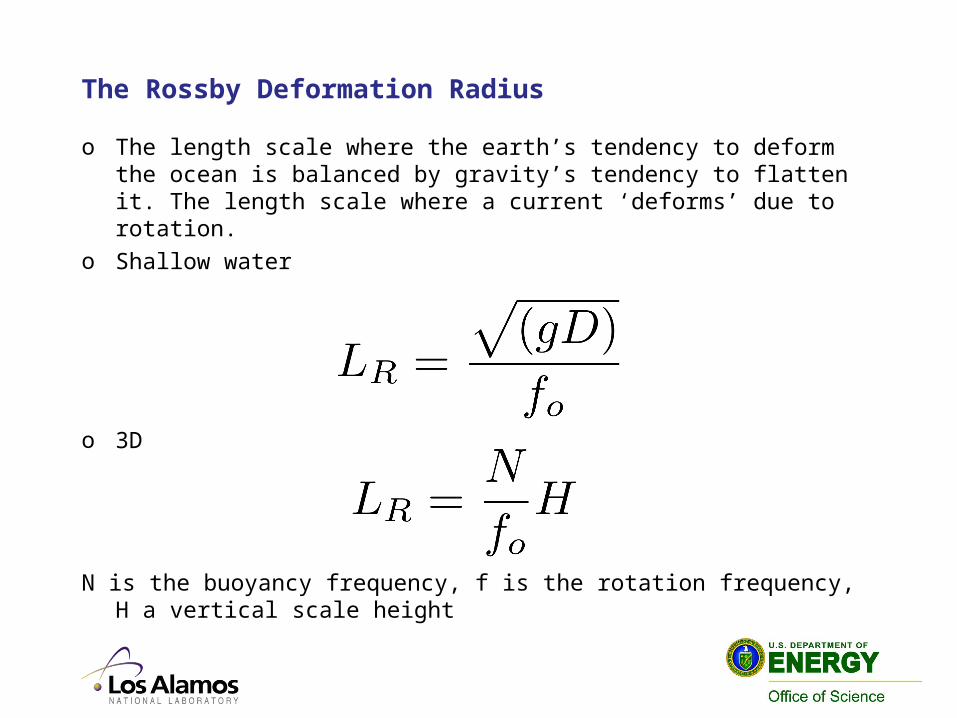
The Rossby Deformation Radius

o The length scale where the earth’s tendency to deform the ocean is balanced by gravity’s tendency to flatten it. The length scale where a current ‘deforms’ due to rotation.

o Shallow water

o 3D

N is the buoyancy frequency, f is the rotation frequency, H a vertical scale height

Deformation radius versus grid spacing

Smith, Maltrud, Bryan, Hecht, 2000

o By using measurements of typical length and time scales Charney, based on a paper he published about stability the year before, derived the Quasi-Geostrophic equations which, “Filtered out the fast waves” (Charney, Geof Publ, 1948)

o He used geostrophic balance and hydrostatic balance.o Extensively used to understand the large scale features

of rotating and stratified flow including explaining baroclinic instability. It also is the source of understanding Rossby waves (planetary scale waves).

o Important conceptual model

Separation of Time Scales and Charney

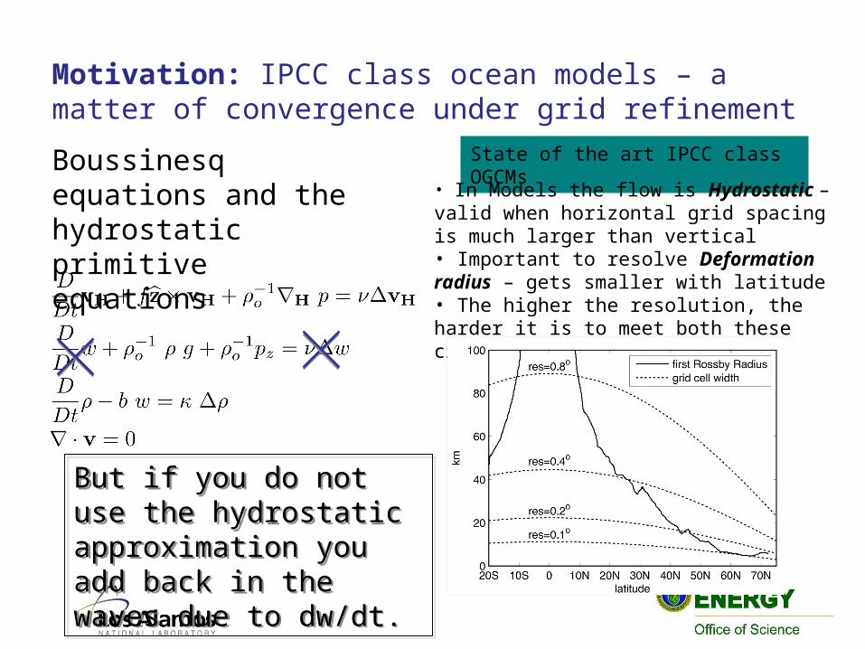
Motivation: IPCC class ocean models – a matter of convergence under grid refinement

State of the art IPCC class OGCMs

• In Models the flow is Hydrostatic – valid when horizontal grid spacing is much larger than vertical• Important to resolve Deformation radius – gets smaller with latitude• The higher the resolution, the harder it is to meet both these criteria.

Boussinesq equations and the hydrostatic primitive equations

But if you do not use the hydrostatic approximation you add back in the waves due to dw/dt.

But if you do not use the hydrostatic approximation you add back in the waves due to dw/dt.

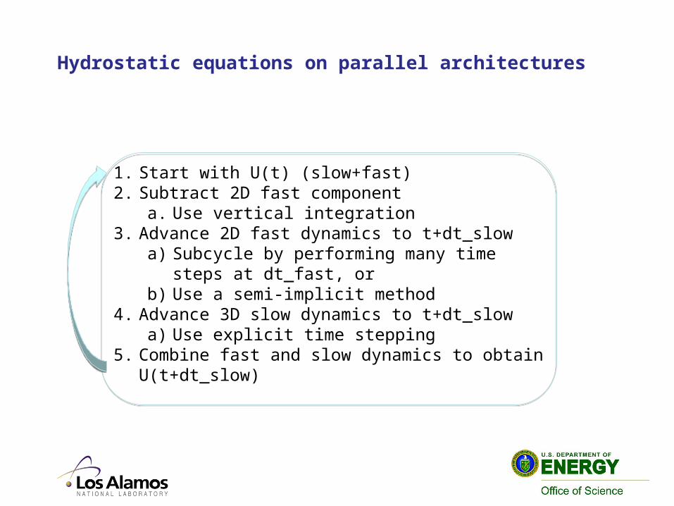
1. Start with U(t) (slow+fast)2. Subtract 2D fast component

a. Use vertical integration3. Advance 2D fast dynamics to t+dt_slow

a) Subcycle by performing many time steps at dt_fast, or

b) Use a semi-implicit method4. Advance 3D slow dynamics to t+dt_slow

a) Use explicit time stepping5. Combine fast and slow dynamics to obtain

U(t+dt_slow)

Hydrostatic equations on parallel architectures

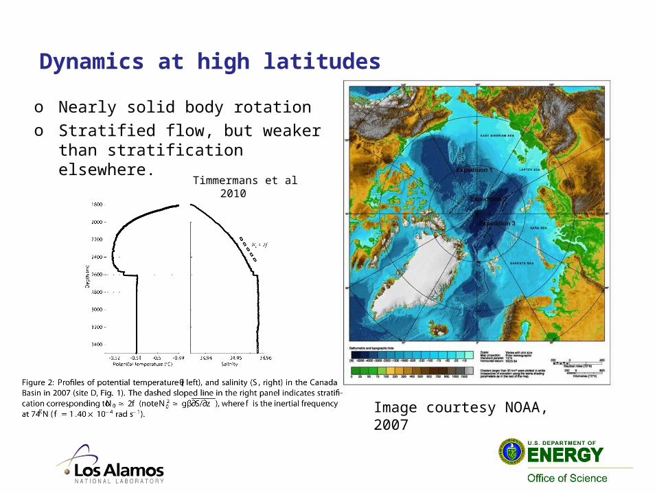
Dynamics at high latitudes

o Nearly solid body rotationo Stratified flow, but weaker than

stratification elsewhere.

Image courtesy NOAA, 2007

Timmermans et al 2010

Low Rossby limiting dynamics in weak stratificationBeth Wingate, Pedro Embid, Miranda Holmes-Cerfon, Mark Taylor

Triply periodic rotating and stratified Boussinesq equations

Embid and Majda, 1996, 1998

Majda and Embid, 1998

Schochet, 1994

Klainerman and Majda 1981

Embid and Majda, 1996, 1998

Majda and Embid, 1998

Schochet, 1994

Klainerman and Majda 1981

Consider the linear waves of this system

Buoyancy Frequency:

Rotation Frequency:

Slow:

Rossby Deformation Radius:

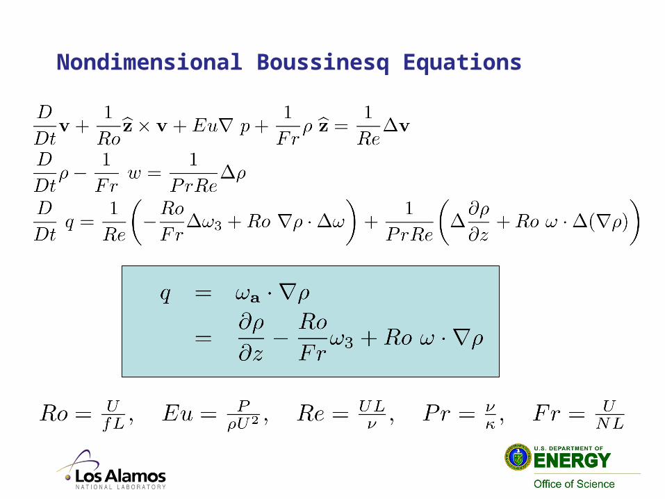
Nondimensional Boussinesq Equations

Conserved Quantities:Total Energy and Potential Enstrophy

In the absence of viscosity and diffusivity:

where

Nonlocal form in a Hilbert Space

Embid and Majda, 1996, 1997

Schochet, 1994

Klainerman and Majda 1981

Hilbert Space X of vector fields u in L that are divergence free and equipped with the L norm.

2

2

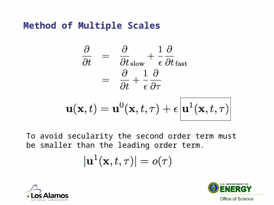
Method of Multiple Scales

To avoid secularity the second order term must be smaller than the leading order term.

Abstract form with slow and fast time scales

To lowest order

Solve for the fast leading order solutions

Solve with Duhammel’s formula and ensure the u1 solution is not large by using the concept of fast wave averaging.

The order 1 solution is a function of the leading order solution:

Where solves:

By direct computation here is the fast wave averaged equation:

Compute the evolution equation for the Fourier amplitudes

The eigenvalues and eigenfunctions of the leading order equations

Look at solutions of the linear problem:

Notice that there is a dispersive mode with zero frequency.

0

gyroscopic/inertial waves

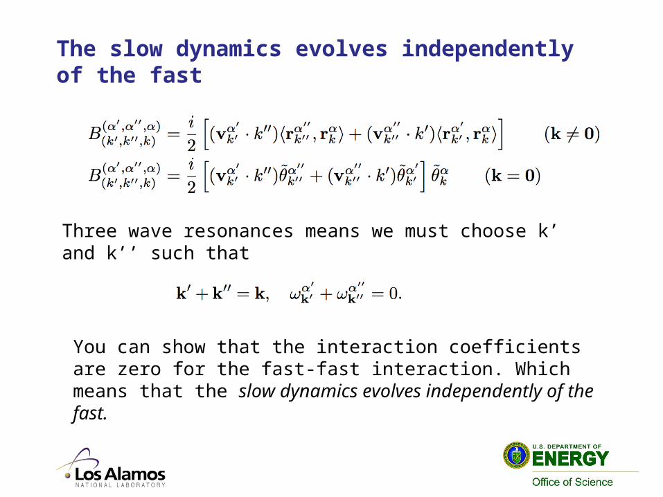
The slow dynamics evolves independently of the fast

Three wave resonances means we must choose k’ and k’’ such that

You can show that the interaction coefficients are zero for the fast-fast interaction. Which means that the slow dynamics evolves independently of the fast.

The new slow equations challenge our ideas of fast and slow dynamics in the ocean. They are nonhydrostatic.

2-D

2-D

3-D

2-D

Taylor-Proudman Theory

Taylor Proudman theorem: In rapidly rotating flow, the flow two-dimensionalizes.

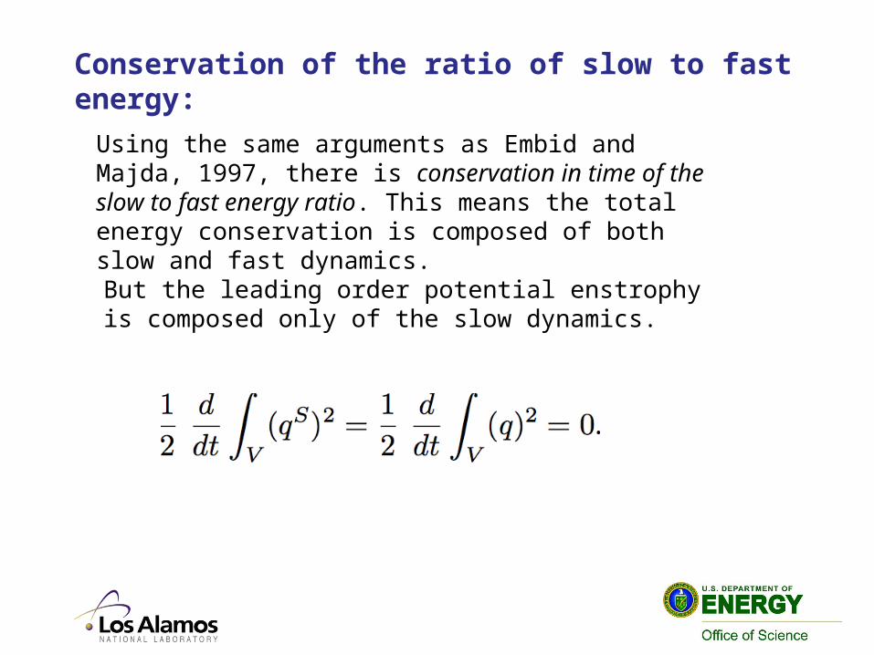
Conservation of the ratio of slow to fast energy:

Using the same arguments as Embid and Majda, 1997, there is conservation in time of the slow to fast energy ratio. This means the total energy conservation is composed of both slow and fast dynamics.

But the leading order potential enstrophy is composed only of the slow dynamics.

High resolution numerical simulations

White noise forcing. Smith and Waleffe, JFM, 2002

Hyperviscosity:

Random Forcing:

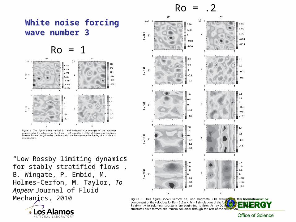
White noise forcing wave number 3

Ro = 1

Ro = .2

“Low Rossby limiting dynamics for stably stratified flows”, B. Wingate, P. Embid, M. Holmes-Cerfon, M. Taylor, To Appear Journal of Fluid Mechanics, 2010

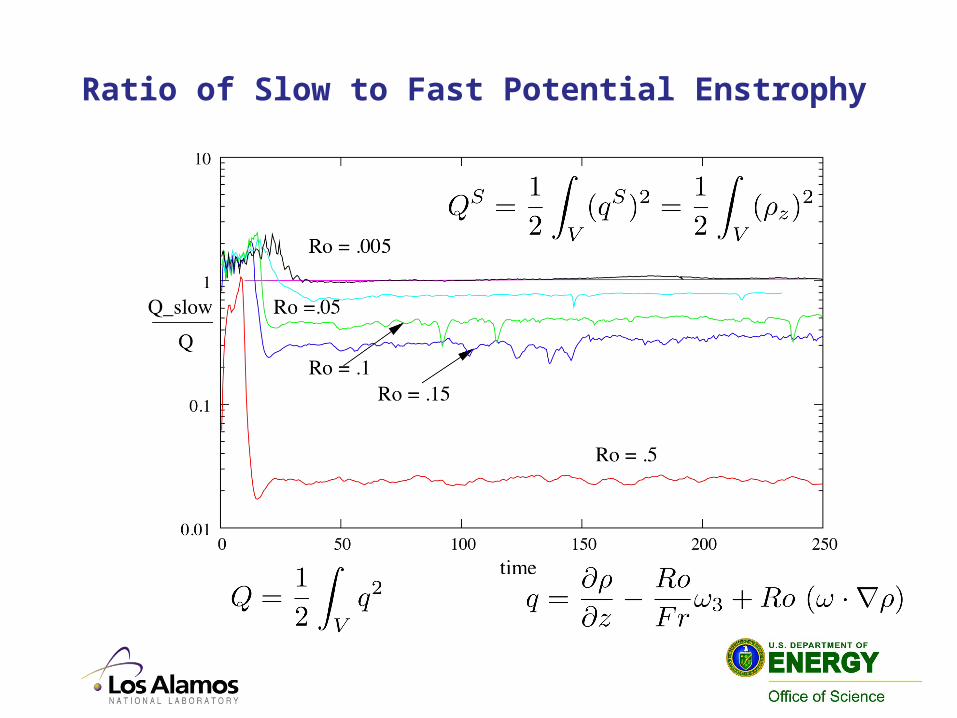
Ratio of Slow to Fast Potential Enstrophy

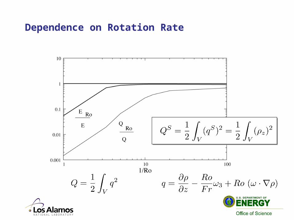
Dependence on Rotation Rate

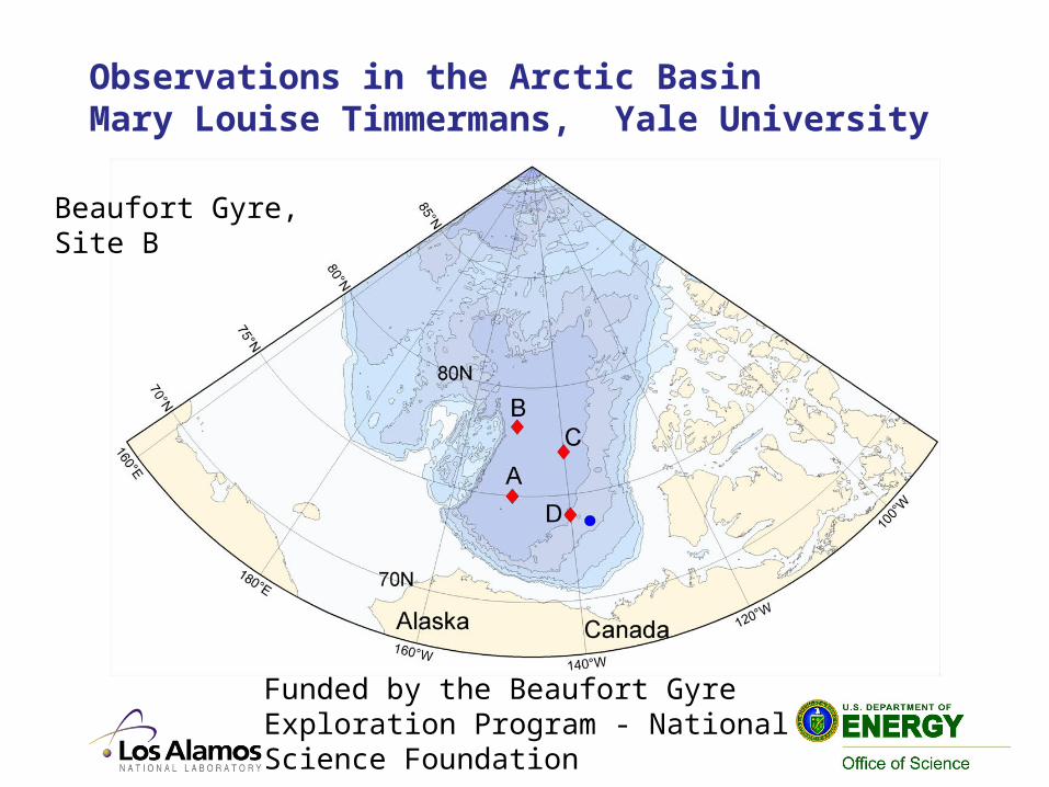
Observations in the Arctic BasinMary Louise Timmermans, Yale University

Beaufort Gyre, Site B

Funded by the Beaufort Gyre Exploration Program - National Science Foundation

Typical Oceanic Conditions at site B

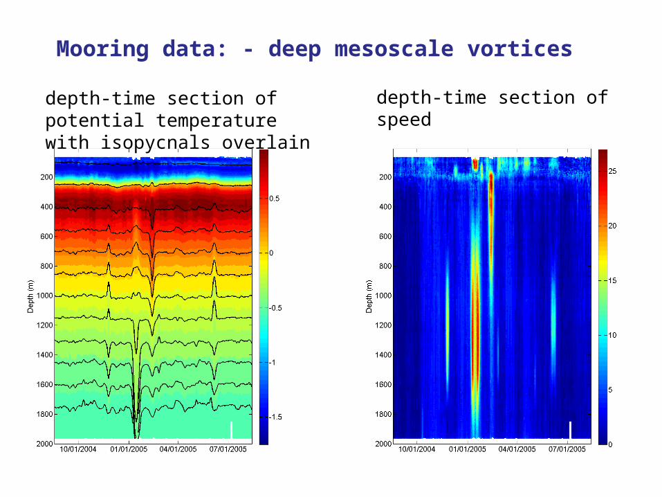
Mooring data: - deep mesoscale vortices

Theme Area? 31

depth-time section of potential temperature with isopycnals overlain

depth-time section of speed

What I’m thinking about for nonhydrostatic ocean and exascale computing

What is fast in most of the ocean (hydrostatic) is slow in areas of weak stratification. Meaning the ocean itself wanders in and out of the parameter space, touching regions where there are separations of time scales but not necessarily QG.

If we are to solve the nonhydrostatic equations for the SLOW mesoscale but step over the fast waves, how do we do it?

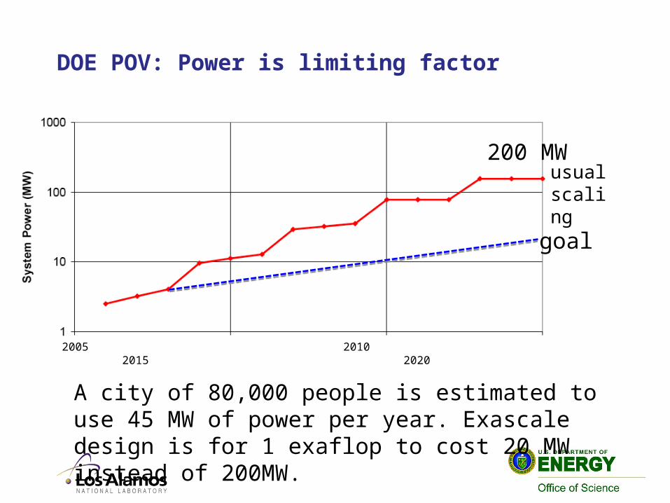
DOE POV: Power is limiting factor

goal

usual scaling

2005 2010 2015 2020

A city of 80,000 people is estimated to use 45 MW of power per year. Exascale design is for 1 exaflop to cost 20 MW instead of 200MW.

200 MW

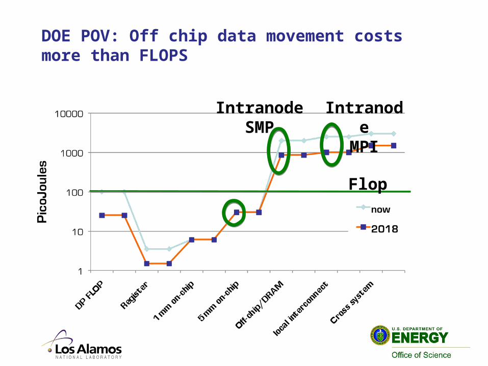
DOE POV: Off chip data movement costs more than FLOPS

IntranodeMPI

IntranodeSMP

Flop

Scientist POV: My life as a Co-Designer Example of the programming model for using CPU + GPU

CPU

Chipset

DRAM

GPU

DRAM

PCIexpress busPCIexpress busHOST DEVICE

Data parallel pieces of an algorithm are executed on the device as KERNELS that are executed as many THREADS grouped together in BLOCKS. BLOCKS grouped together in GRIDS. Each concept has hardware meaning.

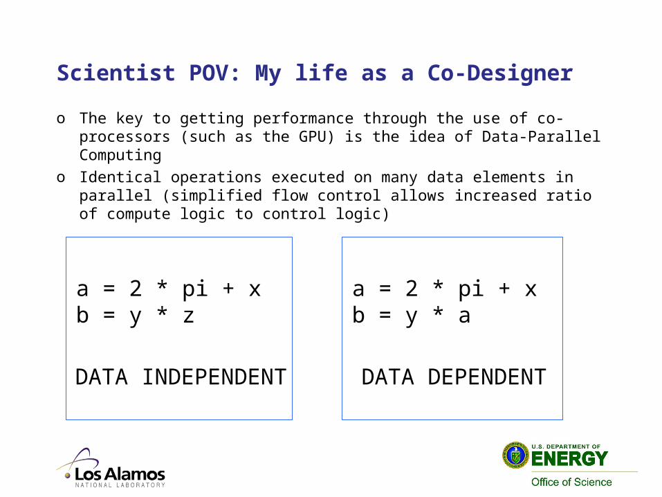
Scientist POV: My life as a Co-Designer

o The key to getting performance through the use of co-processors (such as the GPU) is the idea of Data-Parallel Computing

o Identical operations executed on many data elements in parallel (simplified flow control allows increased ratio of compute logic to control logic)

a = 2 * pi + xb = y * z

a = 2 * pi + xb = y * a

DATA INDEPENDENT DATA DEPENDENT

Scientist POV: My life as a Co-Designer: Example of the programming model for using CPU + GPU

main program{

…… Logic to execute ocean model dynamics

…… Call to ship data in CPU memory to GPU memory

ColumnPhysicsKernal<<<dim3 GridSize, dim3 BlockSize>>>(…)

…… Call to ship GPU memory back to CPU memory}

__global__ ColumnPhysicsKernal(float *x, int *b, …){Int id = blockIDx.x*blockDIM.x+threadID.xA(id) = sin(x(id))}

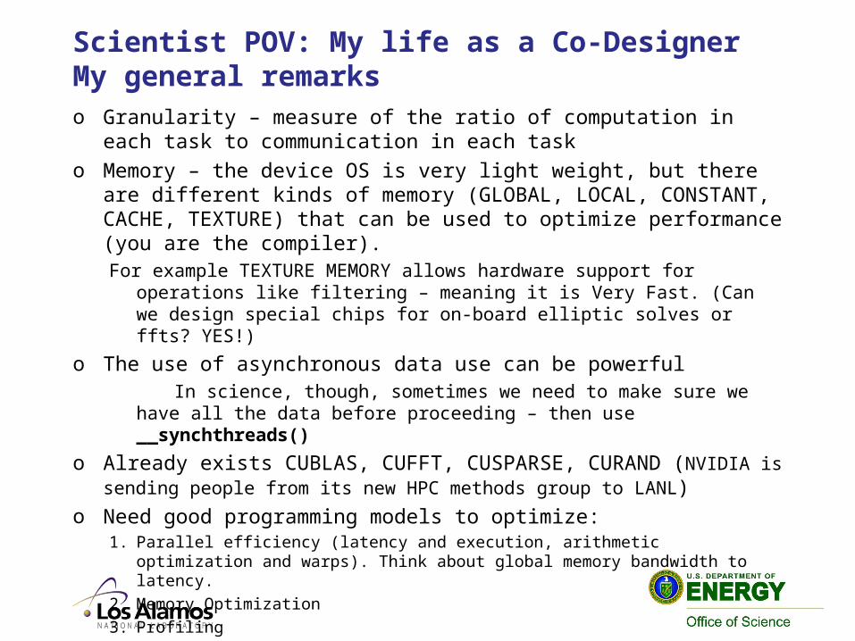
Scientist POV: My life as a Co-Designer My general remarkso Granularity – measure of the ratio of computation in each

task to communication in each tasko Memory – the device OS is very light weight, but there are

different kinds of memory (GLOBAL, LOCAL, CONSTANT, CACHE, TEXTURE) that can be used to optimize performance (you are the compiler). For example TEXTURE MEMORY allows hardware support for

operations like filtering – meaning it is Very Fast. (Can we design special chips for on-board elliptic solves or ffts? YES!)

o The use of asynchronous data use can be powerful In science, though, sometimes we need to make sure we have

all the data before proceeding – then use __synchthreads()

o Already exists CUBLAS, CUFFT, CUSPARSE, CURAND (NVIDIA is sending people from its new HPC methods group to LANL)

o Need good programming models to optimize:1. Parallel efficiency (latency and execution, arithmetic optimization and

warps). Think about global memory bandwidth to latency.2. Memory Optimization3. Profiling

Scientist POV: My life as a Co-Designer More general remarks

o On a heterogeneous machine we can have hardware that perform specific operations. We need to ‘reach through’ all the way to chip designers to do this.

o Considering the original problem from the math/algorithms point of view through the lens of heterogeneous computing1. Our complex climate codes will no longer be dominated by one

numerical method. We may use spectral elements for something, finite volumes for another, we may need to use monte carlo to solve elliptic problems. We may need to throw our current algorithms such as the barotropic/baroclinic splitting away entirely and throw compute cycles at the problem with high order methods. We may need to consider if there is a part of the dynamics that can be considered stochastic.

2. We already do this in the climate model with different methods in the atmosphere, ocean, ice sheets, sea ice. Why not take this further?

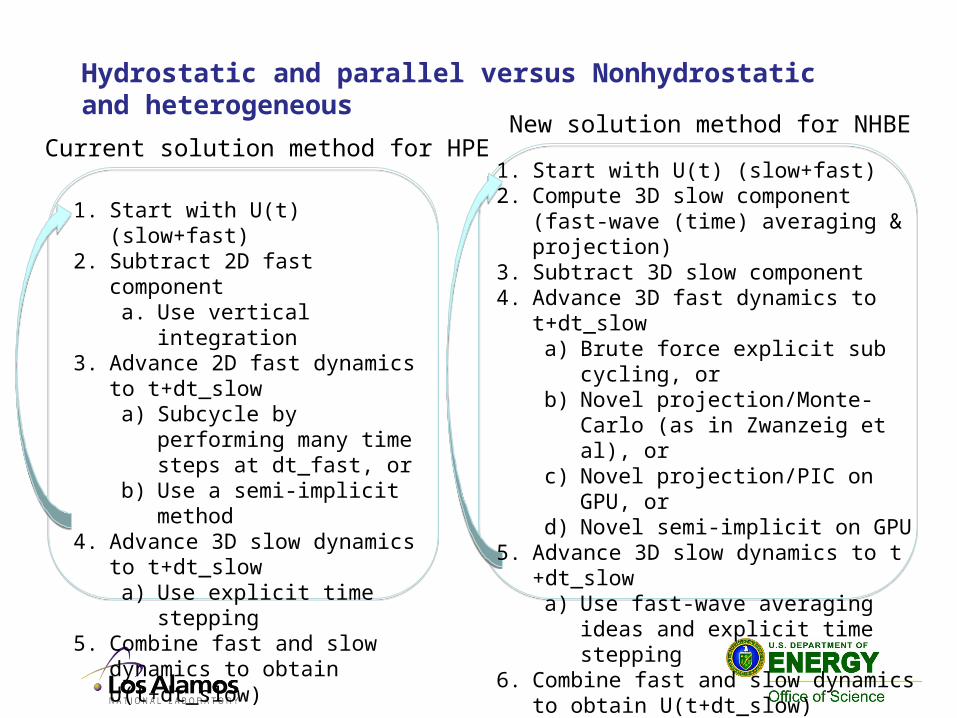
Hydrostatic and parallel versus Nonhydrostatic and heterogeneous

Current solution method for HPE New solution method for NHBE

1. Start with U(t) (slow+fast)2. Subtract 2D fast component

a. Use vertical integration3. Advance 2D fast dynamics to

t+dt_slowa) Subcycle by performing many

time steps at dt_fast, orb) Use a semi-implicit method

4. Advance 3D slow dynamics to t+dt_slow

a) Use explicit time stepping5. Combine fast and slow dynamics to

obtain U(t+dt_slow)

1. Start with U(t) (slow+fast)2. Compute 3D slow component (fast-wave

(time) averaging & projection)3. Subtract 3D slow component4. Advance 3D fast dynamics to t+dt_slow

a) Brute force explicit sub cycling, orb) Novel projection/Monte-Carlo (as in

Zwanzeig et al), orc) Novel projection/PIC on GPU, ord) Novel semi-implicit on GPU

5. Advance 3D slow dynamics to t +dt_slowa) Use fast-wave averaging ideas and

explicit time stepping6. Combine fast and slow dynamics to obtain

U(t+dt_slow)

Summary

o Discussed the mesoscale in contemporary ocean models and our approximations.

o Showed you a new result that suggests there are slow dynamics in weak stratification and they are nonhydrostatic.

o Suggests the nonhydrostatic equations are necessary to predict the mesoscale dynamics.

o Importance of conceptual models in the design of next generation numerical ocean models.

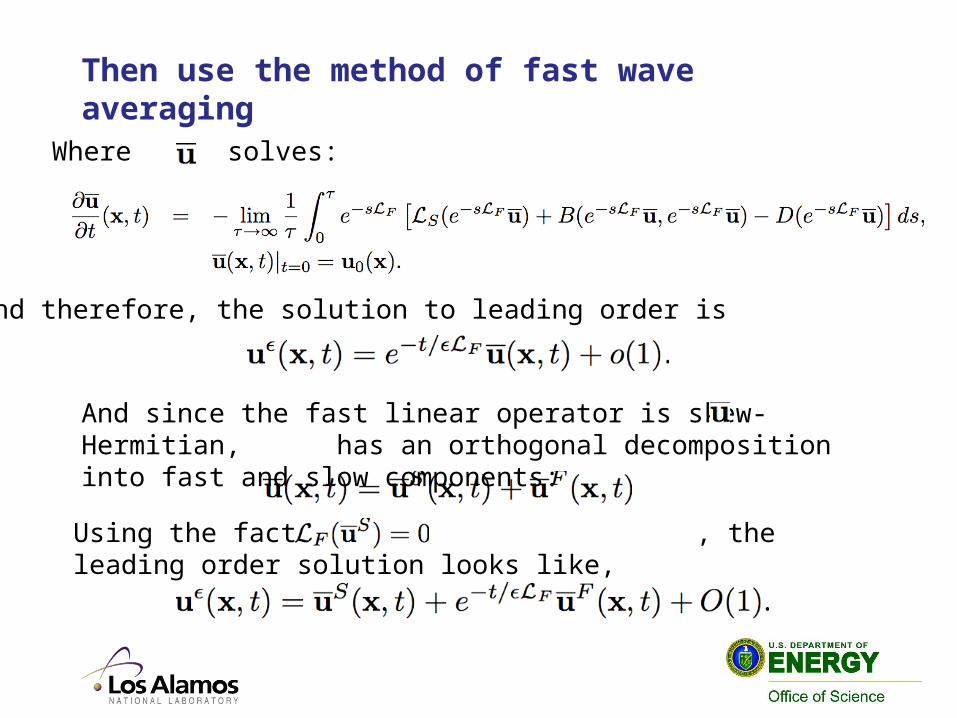
Then use the method of fast wave averagingWhere solves:

And therefore, the solution to leading order is

And since the fast linear operator is skew-Hermitian, has an orthogonal decomposition into fast and slow components:

Using the fact that , the leading order solution looks like,

A key observation is that the fast operator, , is skew-Hermitian in X:.

By the Spectral Theorem, skew-Hermitian operators have purely imaginary eigenvalues and an orthonormal basis of eigenfunctions.

Physically this means the basic normal mode solutions of the equations are wave solutions.

The null space of , , is orthogonal to the range of because the null space is spanned by the eigenfunctions with zero eigenvalues (slow modes) where the range is spanned by the remaining eigenfunctions with non-zero eigenvalues (fast modes).

Derive the equation for the slow dynamics

Knowing the slow dynamics evolves independently of the fast we can find the equations for the slow dynamics by projecting the solution and the equations onto the null space of the fast operator . Then the fast wave averaged equation for the slow modes becomes,

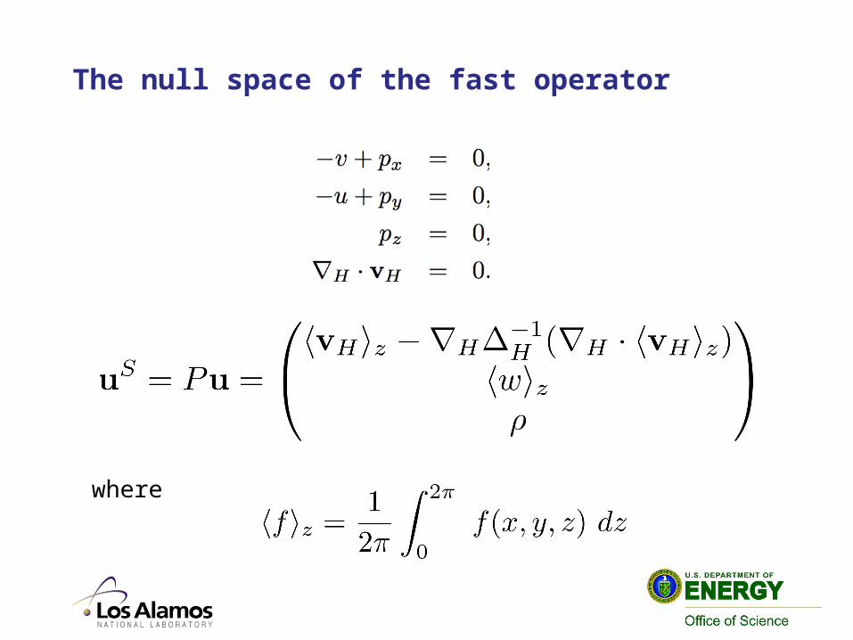
The null space of the fast operator

where

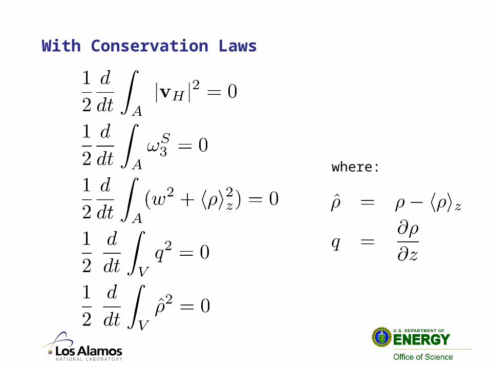
With Conservation Laws

where: