separation of stellar populations by an evolving bar
TRANSCRIPT

MNRAS 469, 1587–1611 (2017) doi:10.1093/mnras/stx947Advance Access publication 2017 April 24
Separation of stellar populations by an evolving bar: implicationsfor the bulge of the Milky Way
Victor P. Debattista,1‹ Melissa Ness,2 Oscar A. Gonzalez,3 K. Freeman,4
Manuela Zoccali5,6 and Dante Minniti6,7,81Jeremiah Horrocks Institute, University of Central Lancashire, Preston PR1 2HE, UK2Max-Planck-Institut fur Astronomie, Konigstuhl 17, D-69117 Heidelberg, Germany3UK Astronomy Technology Centre, Royal Observatory, Blackford Hill, Edinburgh EH9 3HJ, UK4Research School of Astronomy and Astrophysics, Mount Stromlo Observatory, Cotter Road, Weston Creek ACT 2611, Australia5Instituto de Astrofısica, Facultad de Fısica, Pontificia Universidad Catolica de Chile, Av. Vicuna Mackenna 4860, 782-0436 Macul, Santiago, Chile6The Millennium Institute of Astrophysics (MAS), Av. Vicuna Mackenna 4860, 782-0436 Macul, Santiago, Chile7Departamento de Ciencias Fisicas, Universidad Andres Bello, Republica 220, Santiago, Chile8Vatican Observatory, I-00120 Vatican City State, Italy
Accepted 2017 April 19. Received 2017 April 18; in original form 2016 April 15
ABSTRACTWe present a novel interpretation of the previously puzzling different behaviours of stellarpopulations of the Milky Way’s bulge. We first show, by means of pure N-body simulations,that initially co-spatial stellar populations with different in-plane random motions separatewhen a bar forms. The radially cooler populations form a strong bar, and are vertically thin andpeanut-shaped, while the hotter populations form a weaker bar and become a vertically thickerbox. We demonstrate that it is the radial, not the vertical, velocity dispersion that dominates thisevolution. Assuming that early stellar discs heat rapidly as they form, then both the in-plane andvertical random motions correlate with stellar age and chemistry, leading to different densitydistributions for metal-rich and metal-poor stars. We then use a high-resolution simulation,in which all stars form out of gas, to demonstrate that this is what happens. When we applythese results to the Milky Way we show that a very broad range of observed trends for ages,densities, kinematics and chemistries, that have been presented as evidence for contradictorypaths to the formation of the bulge, are in fact consistent with a bulge which formed from acontinuum of disc stellar populations which were kinematically separated by the bar. For thefirst time, we are able to account for the bulge’s main trends via a model in which the bulgeformed largely in situ. Since the model is generic, we also predict the general appearance ofstellar population maps of external edge-on galaxies.
Key words: Galaxy: bulge – Galaxy: evolution – Galaxy: formation – Galaxy: structure –galaxies: bulges – galaxies: kinematics and dynamics.
1 IN T RO D U C T I O N
The origin of the bulge of the Milky Way has been the subjectof considerable discussion. On the one hand, many lines of evi-dence now point to the fact that the Milky Way hosts a bar (deVaucouleurs 1964; Peters 1975; Cohen & Few 1976; Liszt & Bur-ton 1980; Gerhard & Vietri 1986; Mulder & Liem 1986; Binneyet al. 1991; Nakada et al. 1991; Whitelock & Catchpole 1992;Weiland et al. 1994; Paczynski et al. 1994; Dwek et al. 1995;Zhao, Rich & Spergel 1996; Sevenster 1996; Binney, Gerhard &Spergel 1997; Nikolaev & Weinberg 1997; Stanek et al. 1997;
⋆ E-mail: [email protected]
Hammersley et al. 2000). This leads to the opportunity for secu-lar evolution to have sculpted the centre of the Milky Way intothe bulge we see today. Evidence of this comes from the morphol-ogy and kinematics of the bulge. The X-shape of the red clumpdistribution in the bulge is manifested by the bimodal distributionof their distances (McWilliam & Zoccali 2010; Nataf et al. 2010;Saito et al. 2011; Wegg & Gerhard 2013; Gonzalez et al. 2015).This distribution is produced by looking through the near- andfar-side corners of a peanut-shaped bulge (e.g. Li & Shen 2012).Such box-/peanut-shaped (B-/P-shaped) bulges are produced bythe buckling instability of bars (Raha et al. 1991; Merritt & Sell-wood 1994; Bureau & Athanassoula 2005; Debattista et al. 2006)or by orbit trapping (Combes & Sanders 1981; Combes et al. 1990;Quillen 2002; Quillen et al. 2014) and is observed in many external
C⃝ 2017 The AuthorsPublished by Oxford University Press on behalf of the Royal Astronomical Society
1588 V. P. Debattista et al.
galaxies. Li & Shen (2012) showed that a buckled bar model is fullyable to account for this morphology in the Milky Way. Meanwhiledata from the BRAVA, ARGOS and APOGEE surveys have shownthat the bulge is cylindrically rotating (Howard et al. 2008; Nesset al. 2013b, 2016b), which is the typical velocity field producedby bars. A more detailed comparison of a barred simulation withkinematics from the BRAVA survey (Howard et al. 2008; Kunderet al. 2012) by Shen et al. (2010) noted that the velocity and veloc-ity dispersion profiles can be reproduced provided a slowly rotatingbulge component constitutes less than 8 per cent of the disc mass.Thus, these properties all favour the presence of a bulge formed bythe vertical thickening of the bar [see the reviews of Kormendy &Kennicutt (2004) and Fisher & Drory (2016)].
The alternative path to the formation of bulges is their accretionas part of the hierarchical growth of galaxies (Kauffmann, White& Guiderdoni 1993; Guedes et al. 2013). Various lines of evi-dence favouring the existence of such a component in the Galacticbulge have been put forth. Photometric studies of resolved stellarpopulations have generally found uniformly old stars across thebulge, typically older than 10 Gyr (Ortolani et al. 1995; Kuijken& Rich 2002; Zoccali et al. 2003; Ferreras, Wyse & Silk 2003;Sahu et al. 2006; Clarkson et al. 2008, 2011; Brown et al. 2010;Valenti et al. 2013; Calamida et al. 2014). For instance, Clarksonet al. (2011) estimate that any component younger than 5 Gyr mustaccount for less than 3.4 per cent of the bulge. The Milky Way bulgealso exhibits a metallicity gradient in the vertical direction (Zoccaliet al. 2008; Gonzalez et al. 2011; Johnson et al. 2011, 2013). Thisvertical gradient was thought to be impossible if the bulge formedvia the buckling instability. Evidence for an accreted bulge was alsoinferred from the old and metal-poor RR Lyrae at the centre of theGalaxy, which Dekany et al. (2013) showed traced a more axisym-metric, weakly barred shape than the red clump stars. Lastly, thevelocity dispersion of metal-poor stars on the minor-axis above |b|≃ 4◦ becomes flat, while that of metal-rich stars continues declining(Babusiaux 2016), suggesting the existence of a second component.
One interpretation of these seemingly conflicting results isthat the Milky Way has a compound bulge (Athanassoula 2005;Debattista et al. 2005), with both a secular B/P bulge and an ac-creted classical bulge present (Babusiaux et al. 2010; Hill et al. 2011;Zoccali et al. 2014). Many external galaxies have been found to hostcompound bulges. For instance, Mendez-Abreu et al. (2014) foundthat ∼30 per cent of their sample of face-on barred galaxies showedsigns of multiple bulge components, while Erwin et al. (2015) pre-sented a sample of nine galaxies with composite bulges (see alsoErwin et al. 2003). Thus, composite bulges are not rare, and it isconceivable that the Milky Way has one too. A compound bulgecan easily produce the vertical metallicity gradient observed viathe variation of the relative importance of two components (Griecoet al. 2012).
One of the challenges that pure secular evolution models havefaced is why the properties of the bulge should be different for dif-ferent populations (usually defined via the metallicity of the stars).Since gravity cannot act differently on stars of different metallic-ities, a number of studies have postulated that the different stellarpopulations represent different structural components, or perhapsdifferent regions of the initial disc. Martinez-Valpuesta & Gerhard(2013) demonstrate that, contrary to naive expectations, bucklingcan generate a vertical metallicity gradient, consistent with that ob-served, out of steep radial gradients. Di Matteo et al. (2014) insteadconsider pure N-body simulations including a classical bulge andfind that stars initially in the disc as far out as the outer Lindbladresonance of the bar contribute to the boxy bulge, comprising up to
30 per cent of stars at high latitudes. In these scenarios, assumingthat the initial disc has a declining metallicity profile, a puzzlingobservation is that the X-shape is weak or absent in the metal-poorstars (Ness et al. 2012; Uttenthaler et al. 2012; Rojas-Arriagadaet al. 2014). Bekki & Tsujimoto (2011) instead considered the evo-lution of a thin+thick disc model, where the thick disc was metal-poor and the thin disc was metal-rich. In this way, they were ableto build a vertical metallicity gradient in the bulge. Di Matteo et al.(2015) argued that a single thin disc model is unable to produce theobserved split red clump in the metal-rich stars and no split in themetal-poor red clump stars.
As argued by Di Matteo et al. (2015), we do not expect thata single thin stellar disc is able to explain the full range of datauncovered for stars in the bulge because there is nothing to distin-guish different chemical populations. Like those authors, we findthat multiple discs are needed to explain the observational data.However, we show that it is not primarily the disc thickness thatdrives the differences between stellar populations in the bulge, butrather the initial random motion in the disc plane, a situation whicharises naturally in a disc during its early rapid growth phase. In thispaper, we consider both purely collisionless N-body simulationscomprised of multiple stellar populations with different kinematicsand a simulation with star formation, in order to understand how thestructure of the Milky Way’s bulge arises. We discover that stellarpopulations separate (further) in the presence of a bar, a process werefer to as kinematic fractionation. We explore the implications ofthis separation for the morphology, kinematics, ages, chemistry andmicrolensing of the bulge.
This paper is organized as follows. In Section 2, we present asimple dynamical interpretation for why kinematic fractionationoccurs. Section 3 presents a study based on pure N-body simula-tions of kinematic fractionation, showing that the radial velocitydispersion is the main driving factor in the separation and that thevertical velocity dispersion plays a smaller role. We then demon-strate the same behaviour in a simulation with gas and star formationin Section 4. Section 5 compares the trends in the resultant bulgeof this simulation with those in the Milky Way’s bulge, showingthat all the observed trends can be reproduced, with only an addi-tional 5 per cent hot component (a stellar halo) needed to match thekinematics at low metallicity. We also predict new trends for testingfor kinematic fractionation in the Milky Way. Section 6 discussesthese results including making predictions for the metallicity andage distributions of B/P bulges in edge-on galaxies, and ends witha summary of our conclusions.
2 TH E O R E T I C A L C O N S I D E R ATI O N S
Below we present models in which stellar populations with dif-ferent initial in-plane kinematics, but identical density distribution,separate as the bar forms and grows. We refer to this behaviouras kinematic fractionation, in analogy with chemical fractionationproduced by phase transitions. The key result of these simulationsis that the populations with larger initial in-plane random motiongo on to become thicker and less peanut-shaped, and to host weakerbars.
Before presenting these simulations, we seek to understand qual-itatively why radially hotter discs become vertically thicker. Merritt& Sellwood (1994) showed that bending instabilities in discs occurwhen the vertical frequency of stars, ν, exceeds the frequency withwhich they encounter a vertical perturbation, allowing them to re-spond in phase with a perturbation, thereby enhancing it. Bars are themost important source of bending instabilities for two reasons. First,
MNRAS 469, 1587–1611 (2017)

Kinematic fractionation by an evolving bar 1589
because of their intrinsic geometry, bars enforce m = 2 (saddle-shaped) bends, which generally are very vigorous. Secondly, barsraise the in-plane velocity dispersion, but do not substantially alterthe vertical dispersion unless they suffer bending instabilities. Whydoes this matter? Consider the case of a vertical m = 2 perturbationrotating at frequency #p, the pattern speed of the bar. The frequencyat which stars encounter this perturbation is 2(# − #p), where #
is the mean angular frequency of the stars. Thus, stars will supportthe perturbation as long as
ν > 2(# − #p), (1)
enabling it to grow inside co-rotation. If we separate disc starsinto two populations based on their radial random motion, wecan label population ‘h’ (hot) as the one with the larger radialvelocity dispersion and population ‘c’ (cool) the one with thesmaller dispersion. It is well known that the asymmetric drift,$V ≡ Vcirc −
⟨Vφ
⟩≃ xσ 2
R/Vcirc [e.g. Binney & Tremaine (1987),section 4.2.1(a)], where Vcirc is the circular velocity and ⟨Vφ⟩ is themean streaming velocity of the stars and x is a factor that dependson the density distribution and orientation of the velocity ellipsoid;−1 < x < 1 at one disc scalelength. Thus
# ≃ #circ − x
RVcircσ 2
R, (2)
where #circ is the frequency of circular orbits at radius R. Therefore,#h <#c: raising σ R lowers #. While we have assumed near axisym-metry to make this argument, the underlying principle, that hotterpopulations rotate more slowly, holds also when the perturbationis stronger since the mean streaming motion is just one componentsupporting a population against collapse. Stars in population ‘h’satisfy inequality 1 at a smaller ν than those in population ‘c’. Asmaller ν is achieved when the maximum height, zmax, that the starreaches is larger. Since, as a population thickens, ν declines fasterthan # (Appendix A presents orbit integrations which demonstratethis result), a bend in population ‘h’ will saturate at a larger zmax
than in population ‘c’. We conclude that in general radially hotterpopulations can thicken more than radially cooler ones.
This separation of different kinematic populations does not endat the buckling instability. Bars transfer angular momentum tothe halo slowing down in the process (Weinberg 1985; Debattista& Sellwood 1998, 2000; Athanassoula 2002; O’Neill & Dubin-ski 2003). With #p declining and σ R rising, the right-hand side ofequation (1) drops, allowing more stars to respond in phase with fur-ther perturbations. As long as the bar is slowing, therefore, the discwill continue to thicken at different rates for different radial disper-sion populations, allowing the separation of populations to persistin subsequent evolution. As examples of this behaviour, Martinez-Valpuesta, Shlosman & Heller (2006) found that slowing bars thathad buckled already can buckle again, while Debattista et al. (2006)was able to induce buckling in an otherwise stable bar by slowingit down with an impulsively imposed torque.
3 D E M O N S T R ATI O N U S I N G P U R E N- B O DYM O D E L S
The initial conditions usually employed in pure N-body simulationsstudying disc galaxy evolution have generally set up a disc com-posed of a single distribution function, equivalent to a single stellarpopulation. In reality, discs are composed of multiple populationsof different ages with different dispersions; even in the Solar neigh-bourhood, the radial, tangential and vertical velocity dispersionsare all a function of age (e.g. Wielen 1977; Nordstrom et al. 2004;
Holmberg, Nordstrom & Andersen 2009; Aumer & Binney 2009;Casagrande et al. 2011). In the early Universe, disc galaxies weresubject to significant internal turmoil (e.g. Glazebrook 2013), andhad lower mass, which resulted in rapid heating. As a consequence,in young galaxies, the stellar random motion increases rapidly withage over a relatively short period of time. Alternatively, early discsmay form directly hot, with subsequent populations forming incooler, thinner distributions (Kassin et al. 2012; Bird et al. 2013;Stinson et al. 2013; Wisnioski et al. 2015; Grand et al. 2016). Theoutcome of this upside–down evolution is similar: discs with ran-dom motions increasing as a function of age.
In order to explore the effect of the age dependence of randommotions on the evolution of different populations, we first study thebehaviour of multipopulation discs by means of carefully controlledpure N-body (i.e. gasless) simulations where the initial conditionsare comprised of multiple superposed stellar discs with different ini-tial kinematics. We run two types of simulations: one in which mul-tiple stellar discs are exactly co-spatial but have different in-planekinematics (described in Section 3.1), and another set with only twodiscs, with different initial heights (described in Section 3.2).
3.1 Co-spatial discs
In the first set of simulations, we build systems in which the initialdisc is comprised of five separate populations with different in-plane velocity dispersions but identical density distribution. We setup initial conditions using GALACTICS (Kuijken & Dubinski 1995;Widrow & Dubinski 2005; Widrow, Pym & Dubinski 2008). Weconstruct a model consisting of an exponential disc and a Navarro–Frenk–White (NFW) halo (Navarro, Frenk & White 1996), with nobulge component. We truncate this NFW halo as follows:
ρ(r) = 22−γ σ 2h
4πa2h
1(r/ah)γ (1 + r/ah)3−γ
C(r; rh, δrh), (3)
(Widrow et al. 2008). Here, C(r; rh, δrh) is a cutoff function tosmoothly truncate the model at a finite radius, and is given by:
C(r; rh, δrh) = 12
erfc(
r − rh√2δrh
). (4)
Our choice of parameters is σ h = 400 km s−1, ah = 16.7 kpc,γ = 0.873, rh = 100 kpc and δrh = 25 kpc.
We build model discs with an exponential profile:
+(R, z) = +0 exp(−R/Rd) sech2(z/zd), (5)
where Rd is the disc scalelength and zd is the scaleheight. Ourdiscs have Md = 2π+0R
2d = 5.2 × 10¹⁰ M⊙, Rd = 2.4 kpc and
zd = 250 pc. The rotation curve resulting from this set of parametersis shown in the top panel of Fig. 1. We construct five versions ofthis disc density, with different radial velocity dispersion profiles:
σ 2R(R) = σ 2
R0 exp(−R/Rσ ). (6)
We vary the central velocity dispersion, σ R0, fixing Rσ to 2.5 kpc.We select five values of σ R0, 190 km s−1 (disc D1), 165 km s−1 (discD2), 140 km s−1 (disc D3), 115 km s−1 (disc D4) and 90 km s−1
(disc D5). This large range of σ R0 was chosen to enhance the effectof kinematic fractionation; the evolution of further models with anarrower range of σ R0 is qualitatively similar to what we will showhere. The middle panel of Fig. 1 shows the different radial velocitydispersion profiles of the five discs. Although we vary the in-planekinematics of the initial discs, the vertical density profile of eachdisc is identical and therefore the vertical velocity dispersion, σ z,shown in the bottom panel of Fig. 1, is too. We use 6 × 10⁶ particles
MNRAS 469, 1587–1611 (2017)

1590 V. P. Debattista et al.
Figure 1. Top: the rotation curve of the pure N-body models D1–D5. Thedotted (blue) curve shows the halo contribution, the dashed (red) curveshows that of the stars and the solid (black) curve shows the full rotationcurve. Middle: radial velocity dispersions, σR, for discs D1 (red) to D5(blue). Bottom: vertical velocity dispersion, σ z, of the disc in model D5.Models D1–D4 have σ z almost identical to this.
in each disc and 4 × 10⁶ particles in the halo, giving particles ofmass ≃1.1 × 10⁴ M⊙ (disc) and ≃1.7 × 10⁵ M⊙ (halo).
Once we build the five discs, we construct a further two com-pound discs which are superpositions of different subsamples of
D1–D5. In model CU (‘compounded uniformly’), we sample eachof the discs equally. Thus, we extract from each one-fifth of theirparticles and join them together to form a new composite disc withratio D1:D2:D3:D4:D5 set to 1:1:1:1:1. The second disc, modelCL (‘compounded linearly’), samples the discs assuming a linearlydecreasing contribution from D1 to D5 in the ratio 5:4:3:2:1. Thesecomposite systems mimic a system with a continuum of stellar pop-ulations, in the case of CU with a constant star formation rate, whileCL corresponds to a declining star formation rate (assuming that thekinematically hotter populations are older). We therefore refer toeach of disc D1–D5 in models CU and CL as different populations.
Because the overall mass distribution is unchanged by the resam-pling, by the linearity of the Boltzmann and Poisson equations, thecomposite discs CL and CU are also in equilibrium. We evolve thesemodels using PKDGRAV (Stadel 2001), with a particle softening ofϵ = 50 and 100 pc for star and halo particles, respectively. Our basetime-step is $t = 5 Myr and we refine time-steps such that each par-ticle’s time-step satisfies δt = $t/2n < η
√ϵ/ag , where ag is the
acceleration at the particle’s current position; we set η = 0.2. Ourgravity calculation uses an opening angle of the tree code θ = 0.7.
3.1.1 Evolution of single-population discs
Before considering the multipopulation discs, we demonstrate thatthe single-population discs evolve very differently from each otherusing the two most different models, discs D1 and D5. Fig. 2 showstheir evolution. The top panel of Fig. 2 shows the bar amplitude,defined as
Abar =∣∣∣∣
∑i mie
2iφi
∑i mi
∣∣∣∣ (7)
where the sums extend over all star particles in a given disc popu-lation, mi is the mass of the ith particle (which is the same for allstar particles in these pure N-body simulations) and φi is its cylin-drical angle. In both models, the bar forms by 1 Gyr, although thebar in model D1 is best characterized as a very weak oval at thispoint. Later, the two bars reach a semimajor axis of ∼6.5 kpc. Thebar in model D5 buckles at ∼3.7 Gyr, at which point its amplitudedecreases. In model D1 instead an axisymmetric buckling occurs at0.4 Gyr, before the bar forms. We measure the radial profile of theroot-mean-square height of star particles, hz, and average this pro-file to a radius of 2 kpc, ⟨hz⟩; the second panel from the top showsits time evolution. Whereas ⟨hz⟩ evolves mildly in model D5 untilthe bar buckles, in model D1 ⟨hz⟩ rises very sharply from 250 to∼700 pc, while the bar is still forming; thereafter it barely evolvesany further. In model D5 instead the rise in ⟨hz⟩ is initially driven byslow heating by the bar and abruptly by the buckling. The third andfourth panels show the evolution of the radial and vertical velocitydispersions averaged over the same radial range. In model D5, ⟨σ R⟩rises rapidly once the bar forms, while ⟨σ z⟩ increases only slightly.The buckling in model D5 increases ⟨σ z⟩ at the expense of ⟨σ R⟩.Instead, in model D1 a large fraction of the random motion in theplane is transformed into vertical random motion. At later times,both ⟨σ R⟩ and ⟨σ z⟩ evolve very little.
The vertical evolution of a system composed of a single popula-tion is therefore strongly determined by the radial velocity disper-sion before bar formation. A radially hot disc efficiently transformsa large fraction of its in-plane random motion into vertical randommotion. If a hot disc and a cold disc are coincident, a reasonableexpectation is that the cold disc drives the formation of a strong bar,which transforms a large part of the hot disc’s radial random motioninto vertical random motion, thickening the system overall.
MNRAS 469, 1587–1611 (2017)
Kinematic fractionation by an evolving bar 1591
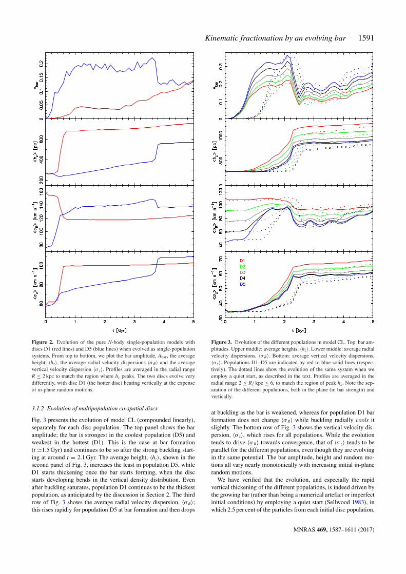
Figure 2. Evolution of the pure N-body single-population models withdiscs D1 (red lines) and D5 (blue lines) when evolved as single-populationsystems. From top to bottom, we plot the bar amplitude, Abar, the averageheight, ⟨hz⟩, the average radial velocity dispersions ⟨σR⟩ and the averagevertical velocity dispersion ⟨σ z⟩. Profiles are averaged in the radial rangeR ≤ 2 kpc to match the region where hz peaks. The two discs evolve verydifferently, with disc D1 (the hotter disc) heating vertically at the expenseof in-plane random motions.
3.1.2 Evolution of multipopulation co-spatial discs
Fig. 3 presents the evolution of model CL (compounded linearly),separately for each disc population. The top panel shows the baramplitude; the bar is strongest in the coolest population (D5) andweakest in the hottest (D1). This is the case at bar formation(t ≃1.5 Gyr) and continues to be so after the strong buckling start-ing at around t = 2.1 Gyr. The average height, ⟨hz⟩, shown in thesecond panel of Fig. 3, increases the least in population D5, whileD1 starts thickening once the bar starts forming, when the discstarts developing bends in the vertical density distribution. Evenafter buckling saturates, population D1 continues to be the thickestpopulation, as anticipated by the discussion in Section 2. The thirdrow of Fig. 3 shows the average radial velocity dispersion, ⟨σ R⟩;this rises rapidly for population D5 at bar formation and then drops
Figure 3. Evolution of the different populations in model CL. Top: bar am-plitudes. Upper middle: average heights, ⟨hz⟩. Lower middle: average radialvelocity dispersions, ⟨σR⟩. Bottom: average vertical velocity dispersions,⟨σ z⟩. Populations D1–D5 are indicated by red to blue solid lines (respec-tively). The dotted lines show the evolution of the same system when weemploy a quiet start, as described in the text. Profiles are averaged in theradial range 2 ≤ R/ kpc ≤ 6, to match the region of peak hz. Note the sep-aration of the different populations, both in the plane (in bar strength) andvertically.
at buckling as the bar is weakened, whereas for population D1 barformation does not change ⟨σ R⟩ while buckling radially cools itslightly. The bottom row of Fig. 3 shows the vertical velocity dis-persion, ⟨σ z⟩, which rises for all populations. While the evolutiontends to drive ⟨σ R⟩ towards convergence, that of ⟨σ z⟩ tends to beparallel for the different populations, even though they are evolvingin the same potential. The bar amplitude, height and random mo-tions all vary nearly monotonically with increasing initial in-planerandom motions.
We have verified that the evolution, and especially the rapidvertical thickening of the different populations, is indeed driven bythe growing bar (rather than being a numerical artefact or imperfectinitial conditions) by employing a quiet start (Sellwood 1983), inwhich 2.5 per cent of the particles from each initial disc population,
MNRAS 469, 1587–1611 (2017)

1592 V. P. Debattista et al.
and from the halo, are drawn from the full system. Each chosenparticle, with phase space coordinates (x, y, z, vx, vy, vz), is thenreplaced by 40 particles as follows:⎛
⎜⎜⎜⎜⎜⎜⎝
x
y
z
vx
vy
vz
⎞
⎟⎟⎟⎟⎟⎟⎠→
19∑
n=0
R(nπ
10
)
⎛
⎜⎜⎜⎜⎜⎜⎝
x
y
z
vx
vy
vz
⎞
⎟⎟⎟⎟⎟⎟⎠+
19∑
n=0
R(nπ
10
)
⎛
⎜⎜⎜⎜⎜⎜⎝
x
y
−z
vx
vy
−vz
⎞
⎟⎟⎟⎟⎟⎟⎠(8)
where R(φ) is the rotation matrix for a rotation by an angle φ aboutthe z-axis. This setup leads to a very low seed m = 2 perturbationout of which the bar must grow, delaying its formation. The dottedlines in Fig. 3 show that the bar forms about 0.5 Gyr later with thisquiet start. The thickening and heating of the different populationsis then also delayed, which would not occur if thickening arises forartificial numerical reasons, and must therefore be driven by the bar.
The evolution of model CU (compounded uniformly) is quali-tatively similar to that of CL. Because the number of particles ineach population is the same in model CU, it makes visual compar-ison between different populations easier. Fig. 4 presents the finaldensity distribution of each population in model CU. In the face-onview, population D1 has a significantly rounder bar with a weakerquadrupole moment, while the bar in population D5 has a strongerquadrupole moment. None the less, the bar has the same size inall five populations. The difference in the vertical structure is evenmore striking; while population D1 has a thick centre and a some-what boxy shape, population D5 is thinner at the centre and thusexhibits a peanut shape. The edge-on unsharp masks in the rightcolumn reveal a photometric X-shape in populations D3–D5 whichis smeared out in populations D1 and D2.
We have verified that the separation of populations is not depen-dent on the presence of very hot populations by running a furthermodel comprised of an equal mix of discs D4 and D5, the twocoolest discs. The two populations separate to a degree comparableto what they did in model CL. Therefore, kinematic fractionationdoes not require very hot populations to be present.
3.2 Evolution of discs with different heights
In this section, we present four different simulations each containingtwo discs of different heights. We use the same version of the thickerdisc in all four simulations. The thinner discs have the same densitydistribution and therefore also the same vertical random motionsin all four cases, but differ in their radial random motions. In thisway, we are able to study the relative importance of vertical andradial random motions to the final B/P bulge morphology of thetwo different populations.
In order to set up initial conditions with discs of different thick-ness, we again use GALACTICS, which allows two discs with differentdensity distributions to be set up. We choose identically the samehalo parameters as in models CL and CU, and again include nobulges in the models. Instead of a pseudo-continuum of populationsas in models CL and CU, we use only two discs, one thinner andthe other thicker. Both discs have a scalelength Rd = 2.4 kpc. Eachdisc has a mass Md = 2.6 × 10¹⁰ M⊙ (i.e. half that of the totaldisc in models CL and CU) and is represented by 3 × 10⁶ particles.One disc has a scaleheight zd = 100 pc (thinner disc), while theother has zd = 400 pc (thicker disc). These two discs are thereforenot to be thought of as the thin and thick discs of a galaxy such asthe Milky Way. Indeed both discs are considerably thinner than theMilky Way’s thick disc and closer to the thin disc (Juric et al. 2008),
which accounts for our terminology ‘thinner’ and ‘thicker’ ratherthan ‘thin’ and ‘thick’. As before, σ 2
R declines exponentially, fromσ R0 = 90 km s−1 for the thicker disc. We produce four thinner discmodels. In T1, the thinner disc is radially cooler than the thickerdisc, while in models T3 and T4, the thinner disc is radially hotter. Inmodel T2, we set up the thinner disc such that it has almost the sameσ R profile as the thicker disc. Fig. 5 shows the initial conditions ofthese systems.
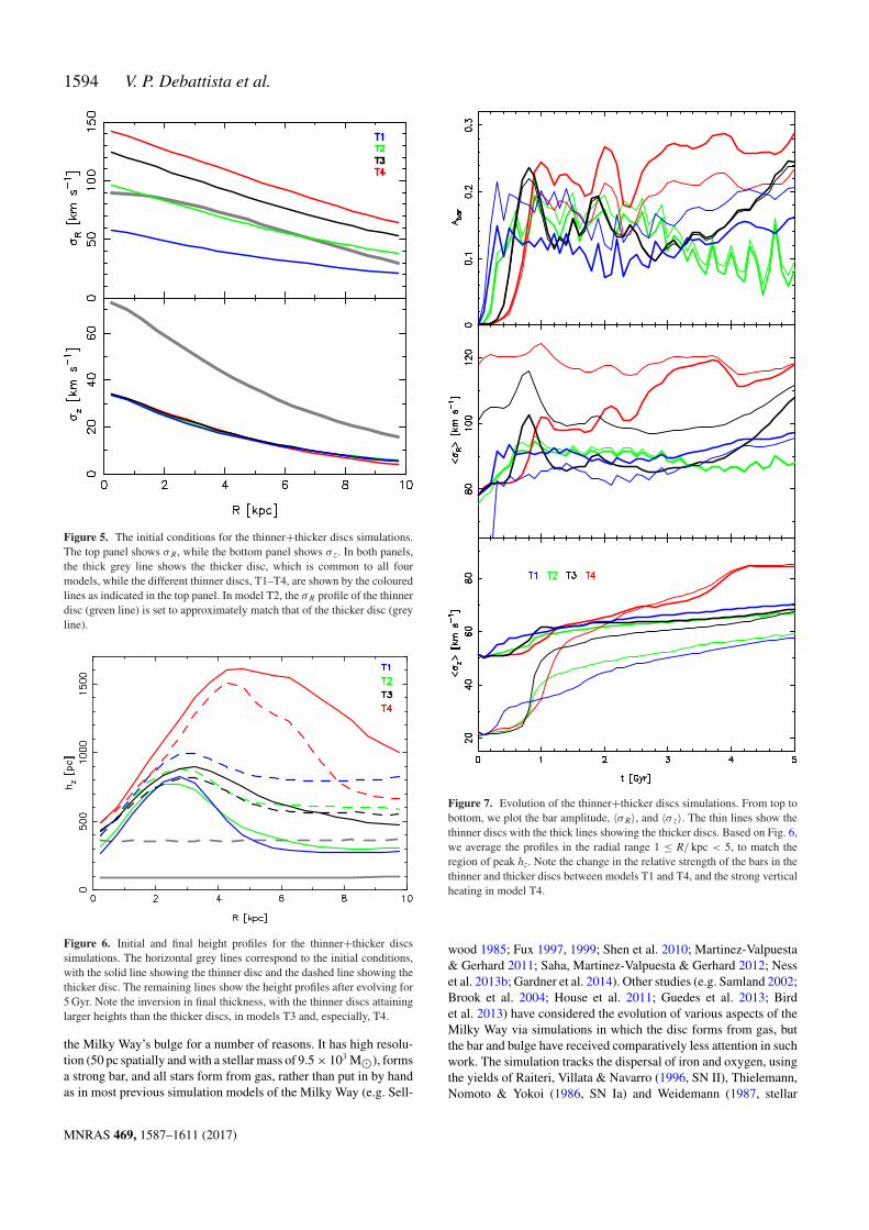
As with models CU and CL, we evolve these models using PKD-GRAV with the same numerical parameters. Fig. 6 compares the finalhz profiles of these models. All four thinner disc models start outwith the same density distribution. The radial extent and degree towhich both discs heat vertically increases from model T1 to T4, i.e.with increasing in-plane random motion of the thinner disc. In mod-els T1 and T2, the thinner disc remains thinner than the thicker disc,but in models T3 and T4, the thinner disc heats to the extent thattheir height becomes larger than that of the thicker disc at the endof the simulation. Fig. 7 shows the overall evolution of the systems.In models T2 and T3, the bar has equal amplitude in both discs,while the bar is stronger in the thinner disc in T1 and in the thicker(but radially cooler) disc in model T4. The velocity dispersionsincrease in all models, with ⟨σ z⟩ increasing rapidly in the thinnerdisc around the time of bar formation. ⟨σ z⟩ increases the most inmodel T4, for which the thinner disc become vertically hotter thanthe thicker disc. Buckling occurs in these models at times rangingfrom 0.3 Gyr (model T1) to 1.1 Gyr (model T4).
Fig. 8 shows face-on and edge-on density maps as well as edge-on unsharp mask images of the thinner and thicker populations inmodel T4. The thicker population, which, initially, has lower radialvelocity dispersion than the thinner population, ends up verticallycooler with a more readily apparent peanut shape, which standsout clearly in the unsharp mask. The thinner disc instead ends upmore vertically extended and hosting a weaker bar with a weakerpeanut shape than the thicker disc. Thus, it is not the initial heightof the disc that is the strongest driver of the final bulge morphology(i.e. whether it is boxy or peanut-shaped), but the in-plane randommotions.
3.3 Summary of the pure N-body simulations
The key insights these pure N-body experiments provide can besummarized as follows:
(i) The formation and evolution of a bar causes co-spatial stel-lar populations, with different initial radial velocity dispersions, toseparate. The initially radially hotter populations are lifted to largerheights than the cooler populations, form a weaker bar, and giverise to a boxy/spheroidal shape, not a peanut shape. The coolerpopulations instead form a peanut shape.
(ii) A thin, radially hot population thickens more than a thick,radially cool population. While it is natural that a radially hot-ter population will also be vertically hotter and thicker, the initialthickness of the disc is not the main driver of the final morphology.Instead, the initial in-plane random motions are more important indetermining the subsequent bulge morphology than is the initialvertical dispersion.
We stress that the initial conditions we have used in these pureN-body simulations are not always meant to represent realistic sys-tems; indeed it would be hard to conceive of a formation scenariowhich leads to a vertically thicker disc being radially cooler than athinner disc. The goal of these experiments has been to show the
MNRAS 469, 1587–1611 (2017)

Kinematic fractionation by an evolving bar 1593
Figure 4. The face-on (left-hand panels) and edge-on (middle panels) surface density of stars in each disc population of model CU at 5 Gyr. These twocolumns share a common density scale indicated by the wedge at top. The right-hand panels show an unsharp mask of the edge-on image using a square kernelof width 1.4 kpc. From top to bottom are shown populations D1 (initially radially hottest) to D5 (initially radially coolest). Decreasing initial σR leads to astronger quadrupole, a thinner disc and a more prominent peanut shape.
relative importance of the vertical and in-plane random motions tothe final morphology.
4 SI M U L ATI O N W I T H STA R FO R M AT I O N
Having explored the effect of different in-plane kinematics withpure N-body simulations, we now examine a simulation in whichthe stars form continuously out of gas, allowing the ages and random
motions (in-plane and vertically), as well as the chemical properties,to be correlated. We consider the evolution of the model presented byCole et al. (2014) and Ness et al. (2014). Briefly, in this simulation, adisc galaxy forms entirely out of gas cooling from a spherical coronaand settling into a disc, triggering continuous star formation. Thisstar-forming simulation, which was evolved with GASOLINE (Wads-ley, Stadel & Quinn 2004), the smooth particle hydrodynamics ver-sion of PKDGRAV, is extremely useful for deciphering the evolution of
MNRAS 469, 1587–1611 (2017)
1594 V. P. Debattista et al.
Figure 5. The initial conditions for the thinner+thicker discs simulations.The top panel shows σR, while the bottom panel shows σ z. In both panels,the thick grey line shows the thicker disc, which is common to all fourmodels, while the different thinner discs, T1–T4, are shown by the colouredlines as indicated in the top panel. In model T2, the σR profile of the thinnerdisc (green line) is set to approximately match that of the thicker disc (greyline).
Figure 6. Initial and final height profiles for the thinner+thicker discssimulations. The horizontal grey lines correspond to the initial conditions,with the solid line showing the thinner disc and the dashed line showing thethicker disc. The remaining lines show the height profiles after evolving for5 Gyr. Note the inversion in final thickness, with the thinner discs attaininglarger heights than the thicker discs, in models T3 and, especially, T4.
the Milky Way’s bulge for a number of reasons. It has high resolu-tion (50 pc spatially and with a stellar mass of 9.5 × 10³ M⊙), formsa strong bar, and all stars form from gas, rather than put in by handas in most previous simulation models of the Milky Way (e.g. Sell-
Figure 7. Evolution of the thinner+thicker discs simulations. From top tobottom, we plot the bar amplitude, ⟨σR⟩, and ⟨σ z⟩. The thin lines show thethinner discs with the thick lines showing the thicker discs. Based on Fig. 6,we average the profiles in the radial range 1 ≤ R/ kpc < 5, to match theregion of peak hz. Note the change in the relative strength of the bars in thethinner and thicker discs between models T1 and T4, and the strong verticalheating in model T4.
wood 1985; Fux 1997, 1999; Shen et al. 2010; Martinez-Valpuesta& Gerhard 2011; Saha, Martinez-Valpuesta & Gerhard 2012; Nesset al. 2013b; Gardner et al. 2014). Other studies (e.g. Samland 2002;Brook et al. 2004; House et al. 2011; Guedes et al. 2013; Birdet al. 2013) have considered the evolution of various aspects of theMilky Way via simulations in which the disc forms from gas, butthe bar and bulge have received comparatively less attention in suchwork. The simulation tracks the dispersal of iron and oxygen, usingthe yields of Raiteri, Villata & Navarro (1996, SN II), Thielemann,Nomoto & Yokoi (1986, SN Ia) and Weidemann (1987, stellar
MNRAS 469, 1587–1611 (2017)

Kinematic fractionation by an evolving bar 1595
Figure 8. The face-on (left-hand panels) and edge-on (middle panels) surface density of stars in the thinner (top row) and thicker (bottom row) disc populationsof model T4 at 5 Gyr. These two columns share a common density scale with the first two columns of Fig. 4. The right-hand panels show an unsharp maskof the edge-on image using a square kernel of width 1.4 kpc. The initially thinner disc ends thicker, with a less peanut-shaped bulge, than the initially thickerdisc, demonstrating that the main driver of the final morphology is not the thickness of the initial disc, but its in-plane random motion.
winds), allowing us to dissect the model not just by age, but also bymetallicity, [Fe/H], and α-enhancement, [O/Fe].
Cole et al. (2014) showed that the model forms between 2 and 4Gyr, slowly growing longer after then (their figs 1 and 2). By 10 Gyr,a B/P-shaped bulge has formed as can be seen in fig. 2 of Ness et al.(2014). Because we are interested in comparing the model to theMilky Way, we scale the model in size and velocity to approximatethe size of the bar and the bulge rotational velocity as seen fromthe Sun, as described in Ness et al. (2014, multiplying coordinatesby 1.2 and velocities by 0.48). We use the same scalefactors at alltimes when presenting this simulation.
4.1 The system before bar formation
At 2 Gyr, the model has already formed 55 per cent of the total finalstellar mass, which is not uncommon for Sb-type galaxies (e.g. Ken-nicutt, Tamblyn & Congdon 1994; Tacchella et al. 2015), althoughon average Milky Way mass galaxies reached half their mass atz ∼ 1–1.4 (Behroozi, Wechsler & Conroy 2013; Patel et al. 2013;Terrazas et al. 2016; van Dokkum et al. 2013). We measure theproperties of the stellar distribution at this time as a function of thetime of formation, τ , of the stars. We separate stars in 0.5 Gyr binsin τ and from here on refer to each such bin as a separate population.
We emphasize that the stars initially form in a discy distribu-tion. Fig. 9 shows the density distribution of the oldest stellarpopulation, with 0.0 ≤ τ ≤ 0.5 Gyr, at t = 0.5 Gyr, i.e. just af-ter formation. Strong spirals can be seen, as can a few very weakstar-forming clumps. At t = 10 Gyr, this population still retains adiscy character, although the stars have spread out, both radiallyand vertically, considerably.
Fig. 10 shows the average radial, ⟨σ R⟩, and average vertical,⟨σ z⟩, velocity dispersions, for the stars born before 2 Gyr. At 2 Gyr,the older stellar populations are radially and vertically hotter thanthe younger populations. The top row of Fig. 11 maps the av-erage metallicity, ⟨[Fe/H]⟩, at t = 2 Gyr. ⟨[Fe/H]⟩ rises rapidlyin the first 2 Gyr. For all populations, the central ∼500 pc is moremetal-rich with a small [Fe/H] gradient outside this region. A small-scale (∼0.5 kpc) bar is evident in the mass distribution, which pro-
Figure 9. The oldest stellar population (0.0 ≤ τ ≤ 0.5 Gyr) at t = 0.5 Gyrin the star-forming simulation. The distribution of these stars is discy andthin at formation, not a thick spheroid.
vides the seed around which the larger bar grows. We also exam-ined maps of the average α-abundance, ⟨[O/Fe]⟩. These show that⟨[O/Fe]⟩ drops rapidly with increasing τ .
Thus overall, at 2 Gyr, before the bar has formed, the ageof a stellar population correlates with ⟨σ R⟩, and ⟨[O/Fe]⟩, andanticorrelates with ⟨[Fe/H]⟩. These dependencies on age im-ply that σ R correlates with chemistry, which we show explicitlyin Fig. 12.
Therefore, on the basis of the pure N-body simulations, we ex-pect that the bar will cause the different populations to separatemorphologically, forming a stronger bar in the younger, metal-rich
MNRAS 469, 1587–1611 (2017)

1596 V. P. Debattista et al.
Figure 10. The evolution of ⟨σR⟩ (top), and ⟨σ z⟩ (bottom) in the star-forming simulation. The different τ populations are indicated in the toppanel. Averages are taken over the radial range 1.5 ≤ R/ kpc ≤ 3. Note thatat 2 Gyr (marked by the filled circles), as the bar starts forming, the radialand vertical dispersions increase with τ .
Figure 12. The (anti)correlation between ([Fe/H]) [O/Fe] and σR att = 2 Gyr, before the bar has formed in the star-forming simulation. Theserelations arise because σR, [Fe/H] and [O/Fe] all evolve with time.
Figure 11. Maps of ⟨[Fe/H]⟩ at t = 2 Gyr (top row) and at t = 10 Gyr (bottom row) for different τ populations as indicated at the top right of each map (fromleft to right, 0.0 ≤ τ/ Gyr ≤ 0.5, 0.5 ≤ τ/ Gyr ≤ 1.0, 1.0 ≤ τ/ Gyr ≤ 1.5 and 1.5 ≤ τ/ Gyr ≤ 2.0), in the star-forming simulation. The colour scale, indicatedby the wedge beside each map, is common to all panels and spans −1.5 ≤ [Fe/H] ≤ 0.2. Contours indicate the surface density of the different populations.The metallicity of populations rises rapidly with τ .
MNRAS 469, 1587–1611 (2017)

Kinematic fractionation by an evolving bar 1597
Figure 13. The azimuthally averaged rotation curve of the star-formingsimulation after 10 Gyr.
populations and a more ellipsoidal distribution in the older, metal-poor populations. As with σ R, σ z also correlates with age, as ex-pected since dispersions increase continuously at this time. Thus, σ z
will also correlate with chemistry, but the driver of the separation ofpopulations will be σ R, not σ z, as we showed in Section 3.2 abovefor the pure N-body simulations.
4.2 The final system
The azimuthally averaged rotation curve of this model at 10 Gyris shown in Fig. 13. This exhibits a central peak which then dropsoff and flattens. Because we are studying the bulge of the model,our velocity scaling is determined by comparing the bulge with thatof the Milky Way, which has a rather flatter rotation curve (e.g.Bland-Hawthorn & Gerhard 2016; Li et al. 2016). Further out, therotation velocity of our model is lower than that of the Milky Way.
4.2.1 Velocity dispersions
Fig. 10 shows the evolution of ⟨σ R⟩ and ⟨σ z⟩. We average in therange 1.5 ≤ R/ kpc ≤ 3 in order to avoid the effects of the nucleardisc (Cole et al. 2014; Debattista et al. 2015). The formation ofthe bar raises ⟨σ R⟩ sharply, while ⟨σ z⟩ increases more slowly. Asin the pure N-body simulations, ⟨σ R⟩ of the different populationsevolve towards each other, while their ⟨σ z⟩ remain separated, withcontinued late time heating driven by the growing bar. While we findno single violent buckling event like in the pure N-body simulations,small-scale bends in the disc can be detected after 2 Gyr, whichcontribute to the vertical heating of the inner disc.
4.2.2 Vertical distribution
The top panel of Fig. 14 plots profiles of hz for the different τ pop-ulations. All populations thicken considerably outside R = 500 pcbetween 2 and 10 Gyr, with the height of the oldest populationroughly doubling at R = 2 kpc. For stars with 2 ≤ τ/ Gyr ≤ 4, theprofile is locally peaked at R ≃ 1.6 kpc rather than monotonicallyincreasing, indicating that these younger populations are peanut-shaped.
The bottom panel of Fig. 14 plots the vertical density profilesalong the minor axis of the disc at 10 Gyr for different τ populations,
Figure 14. Top: vertical height of stars at t = 2 Gyr (dashed lines) andat 10 Gyr (solid lines) for the different τ populations in the star-formingsimulation. The younger stars have a prominent local peak at R ∼ 1.7 kpc,coinciding with their stronger peanut shape. Bottom: vertical density profilealong the minor axis of the disc at 10 Gyr. The profiles are normalized to thecentral density of the oldest population. Colours are as in the top panel. Thered lines show four bins, of equal width in τ , of stars born at 2 ≤ τ/ Gyr ≤ 4.The younger populations extend to lower height than the older populations.
normalized by the mid-plane density of the oldest population. Theoldest population is clearly the one that extends the furthest inheight and we have verified that still younger populations reacheven lower height. The density of the oldest population peaks atz ≃ 200 pc rather than at the mid-plane. This may be related to theboxy-core structure reported by Li & Shen (2015).
4.2.3 Bar strength
The left-hand panels of Fig. 15 show the final projected stellarsurface density in different populations. There is a clear trend forthe stellar distribution to become more strongly barred the later thestars formed. For stars formed before the bar (τ ≤ 2 Gyr), there isa strong dependence of bar strength on age. The bottom panel ofFig. 16 shows the evolution of bar amplitude, Abar, as a function ofτ . Populations with τ < 1.5 Gyr end up in a weaker bar comparedwith populations that form later. The various populations with 2 ≤τ/ Gyr ≤ 4 have very similar global amplitude. The bar amplitude
MNRAS 469, 1587–1611 (2017)

1598 V. P. Debattista et al.
Figure 15. The face-on (left two columns) and edge-on (middle two columns) surface density distribution for different τ populations, as indicated, in thestar-forming simulation at t = 10 Gyr. The right two columns show a cross-section with |y| ≤ 0.2 kpc through the edge-on views of the middle panels. Inthe edge-on panels, the bar is perpendicular to the line of sight (i.e. it is viewed side-on). Note that slightly different spatial scales are used for the face-onand the edge-on views. The quadrupole moment and peanut shape both increase rapidly with τ .
Figure 16. Top: final radial m = 2 amplitude, a2 (m = 2 Fourier amplitudein radial bins), of the surface density of stars in different τ populations inthe star-forming simulation. Bottom: the evolution of bar amplitude, Abar,for different τ populations, as indicated. Globally and at each radius, the baris weakest in the oldest stellar populations. The red lines show four bins, ofequal width in τ , of stars born at 2 ≤ τ/ Gyr ≤ 4.
of the old populations evolves in parallel with that of the younger,cooler populations without ever becoming as strong.
The top panel of Fig. 16 presents the radial profile of the m = 2Fourier moment, a2, showing that the peak amplitude decreaseswith age. Populations formed during 2 ≤ τ/ Gyr ≤ 4 also havedifferent profiles, in spite of their equal overall bar strength, withpeak amplitude increasing with τ . In Fig. 15, this is directly evidentas an increasingly elongated density distribution. None the less thebar has the same semimajor axis size for all populations.
4.2.4 Peanut shape
The middle and right-hand panels of Fig. 15 show the edge-ondistribution of different τ populations, with the bar viewed side-on.As τ increases, the disc becomes thinner, particularly at the centreand the shape changes from boxy to peanuty, in agreement withthe radial profiles of hz shown in the top panel of Fig. 14. Thevery oldest populations have a thick, boxy spheroidal shape. Theyounger populations are thinner at the centre, resulting in a peanutstructure. As with the bar strength, this result is in agreement withthe pure N-body simulations.
4.2.5 Chemistry
The bottom row of Fig. 11 shows maps of ⟨[Fe/H]⟩ at t = 10 Gyr,which can be compared with the maps in the top row at t = 2 Gyr.The central ⟨[Fe/H]⟩ remains high, although it is distributed over aslightly larger region than at 2 Gyr. Other ⟨[Fe/H]⟩ gradients withineach τ population are largely erased, evidence of the significantmixing over this region.
The top panel of Fig. 17 shows the vertical ⟨[Fe/H]⟩ profiles onthe bar’s minor axis. A non-zero gradient is present which at large|z| is dominated by the oldest population. The vertical ⟨[Fe/H]⟩ gra-dient for all stars varies with |z|, becoming flatter with height. Thebottom panel shows similar profiles for ⟨[O/Fe]⟩. The oldest popu-lation is very α-enhanced, dropping rapidly with τ . The ⟨[O/Fe]⟩ ofall stars is low near the mid-plane where stars are still forming butis quickly dominated by the oldest stellar population by ∼400 pc. Inboth panels, the profile within each τ bin is flatter than the overall
MNRAS 469, 1587–1611 (2017)

Kinematic fractionation by an evolving bar 1599
Figure 17. Vertical profiles of stellar chemistry on the minor axis of the bar(with R < 0.3 kpc) at 10 Gyr for different populations in the star-formingsimulation. The top panel shows ⟨[Fe/H]⟩, while the bottom one shows⟨[O/Fe]⟩. The total profiles are indicated by the orange lines. The stronggradients are largely due to the different vertical extent of different agepopulations, not to internal gradients within each τ population, which arequite shallow. The red lines show four bins, of equal width in τ , of starsborn at 2 ≤ τ/ Gyr ≤ 4.
profile, indicating that the overall steep gradients in ⟨[Fe/H]⟩ and⟨[O/Fe]⟩ are produced by variations in the relative densities of dif-ferent age populations. Once the oldest population dominates thevertical profile, the chemical gradients become much flatter.
4.2.6 Dependence of height on metallicity
The top panel of Fig. 18 plots the height profiles of stars for differentbins in [Fe/H]. The metal-rich stars comprise a thinner distributionthan do the metal-poor ones. A peak is present at R ≃ 1.6 kpc in thehigh metallicity hz profile, whereas it rises monotonically for themore metal-poor stars. The peak in the metal-rich stars is a signatureof the peanut-shaped distribution in the younger populations, andthe absence of a peak in the lowest [Fe/H] stars is consistent withthe absence of a peanut shape in old stars. The height profilesfor different [O/Fe] bins are qualitatively similar, with the [O/Fe]-rich population monotonically increasing in height, whereas the[O/Fe]-poor population exhibits a local peak. Bearing in mind theanticorrelation between age and [Fe/H], and the correlation with[O/Fe], Figs 14 and 18 tell a consistent story.
4.3 Synthesis of the pure N-body and star-forming simulations
We have shown that the evolution of both the kinematics and themorphology of the star-forming simulation are consistent with those
Figure 18. Profiles of the vertical height for different [Fe/H] (top) and[O/Fe] bins (bottom) at 10 Gyr in the star-forming simulation. Peaks, asso-ciated with a peanut, rather than boxy, shape, are evident at high [Fe/H] andlow [O/Fe].
of the pure N-body simulations: populations with smaller initialin-plane velocity dispersions end up vertically thinner with a pro-nounced peanut shape and a strong bar. Conversely, the hotter pop-ulations form a thicker distribution with a boxy, not peanut, shapeand with a bar that has a significantly weaker quadrupole moment.The pure N-body simulations have, by their nature, no chemistrybut if we reasonably assume that the high σ R populations are older,then we expect them to have lower [Fe/H] and higher [O/Fe], asin the star-forming simulation. Then, the pure N-body simulationswould predict a strong peanut shape in the metal-rich populationand a weak bar with a boxy bulge in the oldest, metal-poor pop-ulation. The evolution of the bulge in the star-forming simulationcan therefore be understood simply as resulting from the separationinduced by differences in in-plane kinematics at bar formation.
5 A P P L I C ATI O N TO TH E M I L K Y WAY
Having understood how kinematic fractionation gives rise to mor-phological and kinematic differences between different stellar pop-ulations, we now explore whether the resulting trends can explainobservations of the Milky Way’s bulge by comparing the star for-mation model with the Milky Way. We also take this opportunityto predict trends that have not been observed before. We scale themodel in the same way as above and view the model from the Sun’sperspective, using the standard Galactic coordinates (l, b). We as-sume that the Sun is 8 kpc from the Galactic Centre, placing theobserver at y = −8 kpc, and orienting the bar at an angle of 27◦ to
MNRAS 469, 1587–1611 (2017)
1600 V. P. Debattista et al.
the line of sight (Wegg & Gerhard 2013). We emphasize that in thissection we are only interested in understanding trends that arise inthe Milky Way’s bulge, not in matching them in detail.
5.1 Caveats about the model
Before comparing the model with the Milky Way, it is important tomention some limitations of the model. The model is very usefulfor interpretating global trends, but should not be construed as adetailed model of the Milky Way, even after we rescale it. It suffersfrom a number of limitations which preclude efforts to test the modelin a detailed quantitative way. One important difference is that theX-shape is less prominent in the model than in the Milky Way, andrises to smaller heights. This is possibly due to the fact that the barhas not grown quite as much as in the Milky Way. The bar in themodel has a radius of ∼3 kpc (Cole et al. 2014), while the bar in theMilky Way extends to ∼4.5–5 kpc (Wegg, Gerhard & Portail 2015).The relatively high gas inflow rate to the centre of the model, withthe attendant angular momentum transport and high star formationrate, is probably the source of this slow growth. Cole et al. (2014)showed that this gas inflow produces a nuclear disc, which De-battista et al. (2015) proposed is the origin of the high-velocitypeaks seen in the mid-plane line-of-sight velocity distributionsat l ≃ 6◦–8◦ in the APOGEE data (Nidever et al. 2012). (Alterna-tively Aumer & Schonrich 2015, proposed that these high-velocitypeaks are produced by young stars trapped by the bar from the disc.)
A second limitation of the model is in its chemical evolution.The simulation did not include the diffusion of metals between gasparticles, without which too many low-metallicity stars form at allages. This has the effect of broadening the metallicity distributionfunction and of weakening the trends between metallicity and age.With metal diffusion, a tighter correlation between age and chem-istry would have resulted, making the chemical separation by thebar even stronger. Also, while the yields we use for the [Fe/H]enrichment have been shown to lead to very good matches to themetallicity distribution functions across the Milky Way (Loebmanet al. 2016), the oxygen yields may have significant offsets (e.g.Loebman et al. 2011).
Lastly, and most obviously, the simulation was only run for 10Gyr. However by the end of the simulation, the model has longbeen in a phase of slow secular evolution, growing slowly whilecontinuing to form stars.
5.2 X-shape
Several of the currently known morphological properties of theMilky Way bulge are based on the magnitude measurement of redclump stars. A number of studies have used bulge red clump starsfrom the Two Micron All-Sky Survey and the VISTA Variablesin the Via Lactea (VVV) ESO public survey (Minniti et al. 2010)to derive the mean line-of-sight distances across the bulge, thusmapping its 3D shape. This has resulted in the discovery of anX-shaped structure as a bimodal distance distribution (McWilliam& Zoccali 2010; Nataf et al. 2010; Saito et al. 2011; Wegg & Ger-hard 2013; Gonzalez et al. 2015). Li & Shen (2012) showed that apeanut-shaped bulge viewed from the Solar perspective is responsi-ble for this X-shape. By separating red clump stars into metal-rich([Fe/H] > −0.5) and metal-poor ([Fe/H] < −0.5) populations,Ness et al. (2012), Uttenthaler et al. (2012) and Rojas-Arriagadaet al. (2014) determined that metal-poor stars do not follow the bi-modal distance distribution and therefore do not trace the X-shapeof the bulge.
We now investigate the properties of the X-shape in the sim-ulation. Gonzalez et al. (2015) have already compared the model,scaled and oriented the same way as here, with the Milky Way. Theyshowed that the model produced a split red clump at b = −8.5◦ for−2◦ ≤ l ≤ +2◦; at l = +2◦ the bright peak is more prominent, whilethe faint peak is more prominent at l = −2◦. These are the sametrends as observed in the VVV survey and can be explained by anX-shaped overdensity of stars along the line of sight.
In order to test if the model is able to reproduce the trends withmetallicity, we observe the star particles assuming they are redclump stars. Because young, metal-poor stars (caused by the ab-sence of gas metallicity mixing) contaminate the old, metal-poorbins when selecting by metallicity, in this analysis we deconstructthe X-shape by age, rather than by [Fe/H]. The method to derivedistances from red clump stars is based on the construction of theluminosity function of the bulge towards a given line of sight wherethe red clump can be easily identified and its mean magnitude ob-tained (Stanek et al. 1994). We set the absolute magnitude of starsin the model to MK = −1.61, selecting equal numbers of stars inthe magnitude bins 12.3 < K < 12.9 and 12.9 < K < 13.58 (chosento sample the near and far arms of the X-shape with equal numbersof stars, independent of the detailed density distribution, reminis-cent of the ARGOS selection strategy). We convolve the magnitudedistribution with a Gaussian kernel of σ = 0.17 mag to simulatethe intrinsic scatter of the red clump (e.g. Gerhard & Martinez-Valpuesta 2012), and then transform back to distance using thedistance modulus appropriate for 8 kpc.
The bottom row of Fig. 19 shows the distribution of the red clumpstars in the model, at distances from the Sun 6 ≤ Rs/ kpc ≤ 11, forthree different lines of sight on the minor axis (|l| < 2◦), wherethe stars are divided into four age bins. At low latitudes (b ∼ 3◦),the distance distribution generally consists of a single peak for allstellar ages, as expected since the arms of an X-shape only becomesufficiently separated at higher latitudes. No split is present in theoldest stars even at higher latitudes, but one is visible for youngerstars. The separation between the peaks increases and the depth ofthe minima between peaks increases with decreasing stellar age.Both the separation and the depth of the minima also become moreprominent with increasing latitude. The prominence of the X-shapedepends strongly on stellar age, with the older stellar populationsshowing a weak (or no) bimodality and the younger populationsexhibiting a strongly bimodal distance distribution.
We infer that the age dependence in the distribution of stars trac-ing the X-shape qualitatively explains the metallicity dependence ofthe split clump observed in the Milky Way, where the most metal-rich stars show the largest bimodality and stars of [Fe/H] < −0.5show only a single peak in their distance distribution. We identifythe oldest stars in the simulation, which trace the X-shape weakly,if at all, with the metal-poor stars in the Galaxy. Conversely, weidentify the more metal-rich stars in the Milky Way, which do tracethe X-shape, with the slightly younger stars in the simulation.
The bottom row of Fig. 19 also shows that stars younger than7 Gyr in the model also have a split red clump. The percentageof stars in each age bin at each latitude is indicated in each panelof Fig. 19. Stars younger than 7 Gyr contribute <14 per cent ofstars in this region, a number which reflects details of the model’sevolution. In the Milky Way, this fraction would be even lower,since observations based on turnoff studies show that such starscontribute <5 per cent of bulge stars (e.g. Ortolani et al. 1995;Kuijken & Rich 2002; Zoccali et al. 2003; Sahu et al. 2006; Clark-son et al. 2008, 2011; Brown et al. 2010; Valenti et al. 2013). Thecrucial point is that an age difference of just 2 Gyr is sufficient for
MNRAS 469, 1587–1611 (2017)

Kinematic fractionation by an evolving bar 1601
Figure 19. The distribution of red clump stars in the star-forming model, at distances from the Sun in the range 6 ≤ Rs/ kpc ≤ 11, at three different lines ofsight on the minor axis, with the stars divided into age bins. Here, age is defined as 10 Gyr − τ . Top: raw data with no observational error added. Bottom: thehistograms convolved with the intrinsic scatter of the red clump magnitude of σ = 0.17 dex. Younger (metal-rich) red clump stars would appear distributed onan X-shape, while older (metal-poor) ones would not, given the intrinsic scatter. More precise distance measurements however can reveal a weak bimodalityalso in metal-poor populations.
the bulge red clump distributions to change from a single peak to abimodal distribution.
The absence of a bimodal distribution in stars older than 8 Gyris not absolute. We have convolved the magnitude distribution withan intrinsic scatter of σ = 0.17 mag. If the observational uncer-tainty were lower, then even the oldest population exhibits a weaklybimodal distribution. The top row of Fig. 19 presents examples ofdistance distributions unconvolved with any observational uncer-tainty. In this case, even the oldest population (age > 9 Gyr) has abimodal distribution at |b| = 5◦. A prediction that follows is that,with higher distance precision, a weaker split at lower metallicitiesmay also be observed. A second prediction from the unsmootheddata is that, for the younger populations, the stars are distributed intwo distinct distributions, corresponding to the arms of the X-shape,with a near zero density of stars in between. We emphasize that thisparticular prediction is for ages, not [Fe/H] since at any age thedistribution of [Fe/H] is probably not perfectly single-valued.
5.3 Interpretation of the different distributions of Milky Waybulge red clump stars and RR Lyrae
The dependence of bar strength on age, shown in Figs 15 and 16, isdirectly relevant to interpreting the difference in the distribution ofRR Lyrae and red clump stars noted by Dekany et al. (2013). Theadoption of red clump stars as distance tracers includes the entirerange of stellar ages that is found in the Milky Way bulge. On theother hand, RR Lyrae are old stars (Walker 1989). Dekany et al.(2013) investigated the spatial distribution of the oldest populationof the bulge by measuring the distances to RR Lyrae based on theirnear-infrared light curves from VVV photometry. They found adistribution of RR Lyrae in the Galactic bulge that is quite roundand exhibits little evidence of the bar morphology traced by the red
clump stars. Fig. 20 shows the projected mean distance to red clumpstars from Gonzalez et al. (2012) compared to that from RR Lyrae.We used the individual distances to the RR Lyrae from Dekany et al.(2013) to calculate a mean RR Lyrae distance using a Gaussian fitto the distance distribution in each line of sight. The projecteddistance is shown in Fig. 20 as well as the surface density contoursusing the individual distances of the entire RR Lyrae sample fromDekany et al. (2013). Dekany et al. (2013) interpreted the spheroidaldistribution of this old population as evidence for a dynamicallydistinct population that formed separate from the disc in the bulge.
We assess the need for such a composite bulge scenario by mea-suring the mean distances to the simulated stars, in a similar way asdone for the observations. We first select all the stars within the dis-tance range 4 ≤ Rs/ kpc ≤ 12 to sample the integrated populationof the red clump stars observed across the extent of the bulge. Wethen consider only the oldest stellar population with τ ≤ 0.5 Gyrto obtain a sample representative of the oldest population of thebulge, corresponding to the population traced by the RR Lyrae. Wethen measure the mean distances to both samples in (l, b)-spaceat a fixed latitude of 3.5◦ ≤ b ≤ 4.5◦ in 1◦-spaced longitude binsbetween −9◦ ≤ l ≤ +9◦. As we did in comparing with the ob-served X-shape, in order to match the observational uncertainties,we first convert the line-of-sight distance of every star particle toan observed magnitude by adopting an absolute magnitude for thered clump of MK = −1.61 mag (Alves 2000). The magnitude dis-tribution of stars towards each line of sight is then convolved witha Gaussian with σ = 0.17 mag in order to account for the intrinsicscatter of the bulge red clump population (Gonzalez et al. 2011;Gerhard & Martinez-Valpuesta 2012). We then produce a Gaus-sian fit to the magnitude distribution towards each line of sight andretrieve the corresponding mean magnitude of the distribution. Fi-nally, this mean magnitude value is converted back to a distance
MNRAS 469, 1587–1611 (2017)

1602 V. P. Debattista et al.
Figure 20. Face-on projection of the simulated mean line-of-sight distancesfor star particles at 3.5◦ < b < 4.5◦ with ages > 9.5 Gyr (black open circles)and for all the star particles (red open circles) in the star-forming simulation.The projected mean line-of-sight distances of RR Lyrae from Dekany et al.(2013) (black filled circles) for latitudes 3.5◦ ≤ b ≤ 4.5◦ and of red-clumpstars in the same latitude range from Gonzalez et al. (2012, red filled circles)are also shown. The surface density contours of the full RR Lyrae sampleof Dekany et al. (2013) are included in the plot. All distances, for simulatedand observed stars, were calculated adopting an absolute magnitude ofMK = −1.61 mag in order to bring the model to the mean distance of the RRLyrae. The simulation matches the weaker barred distribution of RR Lyraeand stronger bar in the red clump stars seen in the Milky Way’s bulge.
using the same MK value. For the oldest stars, instead, we ignorethe small distance uncertainties. Fig. 20 shows the mean positionsprojected on to the (x, y)-plane for both cases: including all the stars,and selecting only the oldest stars from the simulation.
Purely by measuring distances to the oldest stars, the distanceprofile becomes flatter than when including the entire range ofages, with a remarkable similarity to the RR Lyrae measurementsin the Milky Way. Furthermore, when all the stars of the simula-tion are included, the distance profile becomes steeper and tracesthe position angle of the bar. Thus this result explains the differentmorphological signatures traced by red clump stars and RR Lyraewithin the Galactic bulge, without the need for a second, dynami-cally distinct, component. Instead, the continuum of bar quadrupolemoments, from weak to strong as a function of formation time, isable to explain the observed shape difference.
A natural interpretation of the nearly spheroidal distribution ofthe RR Lyrae stars in the Galactic bulge is that these are olderthan the bar itself. By the time the bar formed, they constituteda radially hotter stellar population, possibly as part of the stellarhalo, and therefore did not acquire a strong quadrupole moment. Aconsequence of this interpretation is that the RR Lyrae should notexhibit a strong peanut shape.
Recently, Kunder et al. (2016) presented radial velocity measure-ments of 947 RR Lyrae from the Bulge RR Lyrae Radial VelocityAssay (BRAVA-RR) survey located in four bulge fields at Galacticlatitude −5◦ < b < −3◦ and longitude |l| < 4◦. Kunder et al. (2016)concluded that the bulge RR Lyrae are part of a separate compo-nent, i.e. a classical bulge or inner halo, based on the null rotationobserved in this population when compared to the RC stars. If this
result is confirmed after extending the rotation curve of the RRLyrae to larger Galactic longitudes (|l| < 10◦), it could suggest thatthe population traced by these stars is linked to the most metal-poor([Fe/H] < −1.0) population of red clump stars that shows a simi-lar kinematic behaviour as observed by the ARGOS survey (Nesset al. 2013b). Here, we showed that the oldest population found inthe model follows a weakly barred distribution. However, we do notfind a velocity difference between RR Lyrae and red clump stars aslarge as that seen in the BRAVA-RR data.
A more continuous change in the orientation of the bar with agehas been measured in bulge Mira variables (Catchpole et al. 2016).Mira variables follow a period–age relationship, with short periodscorresponding to older stars (Wyatt & Cahn 1983), spanning arange of ages from ∼3 Gyr to globular cluster ages. Catchpole et al.(2016) find that the younger (!5 Gyr) Mira variables in the bulge at(l, b) = (±8◦, −7◦) follow a clear bar structure, while the older onesare more spheroidal. The angle of the major axis of the distributionof Miras to the line of sight twists continuously with their period,as would be expected for populations with continuously varyingquadrupole moments (e.g. Gerhard & Martinez-Valpuesta 2012).
5.4 Stellar kinematics
We now compare the kinematics of the bulge as observed inARGOS, selecting stars in the simulation to be within 3.5 kpc ofthe Galactic Centre, as was done for red clump stars (with distanceerrors <1.5 kpc) in ARGOS. The results of this section are not toosensitive to these distance cuts; removing the distance cuts changesthe mean velocities and the dispersions by no more than 10 per cent.
The right column of Fig. 21 shows the rotation and dispersionprofiles in the simulation compared to the ARGOS data, at lati-tudes of b = 5◦, 7.5◦ and 10◦. The rotation for both ARGOS andthe simulation is cylindrical, with very little difference in rota-tion speed at different latitudes. Cylindrical rotation of the Galacticbulge has been observed by several studies (e.g. Howard et al. 2008;Kunder et al. 2012; Ness et al. 2013b, 2016b; Zoccali et al. 2014)and is a generic feature of N-body models of boxy bulges (Combeset al. 1990; Athanassoula & Misiriotis 2002; Saha & Gerhard 2013).The dispersion profiles of the observations and the simulation arealso very similar, peaking in the centre and decreasing with increas-ing longitude. The peak velocity dispersion is observed near thecentre (b ∼ 2◦) on the minor axis, as first reported by the GIBS sur-vey (Zoccali et al. 2014), and decreases with latitude. The model’svelocity dispersion at b = 2◦ is ∼1.5 times the velocity dispersionat 5◦, which is comparable to the fractional difference reported inGIBS (Zoccali et al. 2014) and ARGOS (Ness et al. 2016a). Outsidethe boxy bulge, in the disc (|l| > 15◦), the dispersion is similar atall latitudes.
The ARGOS stars span a metallicity range of −2 < [Fe/H] < 0.5,although 95 per cent of stars have [Fe/H] > −1. The velocity dis-persions of stars vary as a function of their metallicity (Babusiauxet al. 2010; Ness et al. 2013b, 2016b). We investigate these ob-served differences in the kinematics using the stellar age in thesimulation as a proxy for [Fe/H], as we did previously for theX-shape analysis. The second column of Fig. 21 shows the kine-matics of the metal-rich ([Fe/H] > −0.5) ARGOS stars, togetherwith intermediate-age (7 Gyr < age < 8 Gyr) stars in the model.The model stars have kinematics that are qualitatively similar to theobservational trends of the metal-rich stars, with a larger differencein velocity dispersion between 5◦ ≤ |b| ≤ 10◦, and a lower andflatter dispersion profile at higher latitudes, compared to all stars(left column). The ∼10 per cent increase in the velocity dispersion
MNRAS 469, 1587–1611 (2017)

Kinematic fractionation by an evolving bar 1603
Figure 21. The ARGOS data (points with error bars) compared to the star-forming simulation (shaded region showing the sampling uncertainty; the shadinguses the same colour scheme as the ARGOS data points to indicate latitude). Left: all stars in the simulation along a given line of sight. Second column: starswith [Fe/H] > −0.5 compared to model stars with ages between 7 and 9 Gyr. Third column: ARGOS stars with [Fe/H] < −0.5 compared with old modelstars (age > 9 Gyr). Right: the same old stars in the model with a 15 per cent admixture of a hot population as described in the text. This fraction correspondsto 5 per cent of the stellar mass of the bulge; this small addition leads to an excellent match to the observed kinematics of the metal-poor stars.
at b = −5◦ of the intermediate-age stars relative to the full distribu-tion is not observed in ARGOS for the more metal-rich stars. Theorigin of this discrepancy is unclear.
The third column of Fig. 21 compares the metal-poor([Fe/H] < −0.5) ARGOS stars with old (age > 9 Gyr) stars inthe model. The trends observed for this population, including therelatively high and flat velocity dispersion that changes slowly withlatitude, are not reproduced by the model. We have explored a va-riety of age cuts in the model, and all of them fail to match thesekinematic trends. This suggests that the model is missing a compo-nent that can produce these kinematics. A similarly hot population atlow metallicity was found by Babusiaux (2016). In order to explorethis population further, we note that ARGOS finds that stars with[Fe/H] < −1 have a ∼50 per cent rotation velocity and an averagevelocity dispersion ∼120 km s−1 across 5◦ ≤ b ≤ 10◦ (componentD of Ness et al. 2013a). We add such a population to the old stel-lar population in the model. The right column of Fig. 21 showsthe outcome of adding 15 per cent of stars with the properties ofpopulation D from ARGOS (i.e. rotation speed which is 50 per centof the metal-rich stars and a dispersion of 120 km s−1) to the oldpopulation in the model. The qualitative match to the observationsis now very good, with flat, nearly constant velocity dispersion withlongitude and a relatively small drop with latitude. Bearing in mindthat the [Fe/H] < −0.5 population accounts for 30 per cent of allthe ARGOS stars, and that the model needed only ∼15 per cent ofsuch stars to match this behaviour, we conclude that this component
accounts for ∼5 per cent of the mass of the central Milky Way. Thisadditional population is most likely the stellar halo, which mustalso be present in the inner Milky Way. This low contribution of ahot component is significantly more stringent than the estimates ofShen et al. (2010) for the presence of a hot, unrotating component.
5.5 Trends in the age distribution
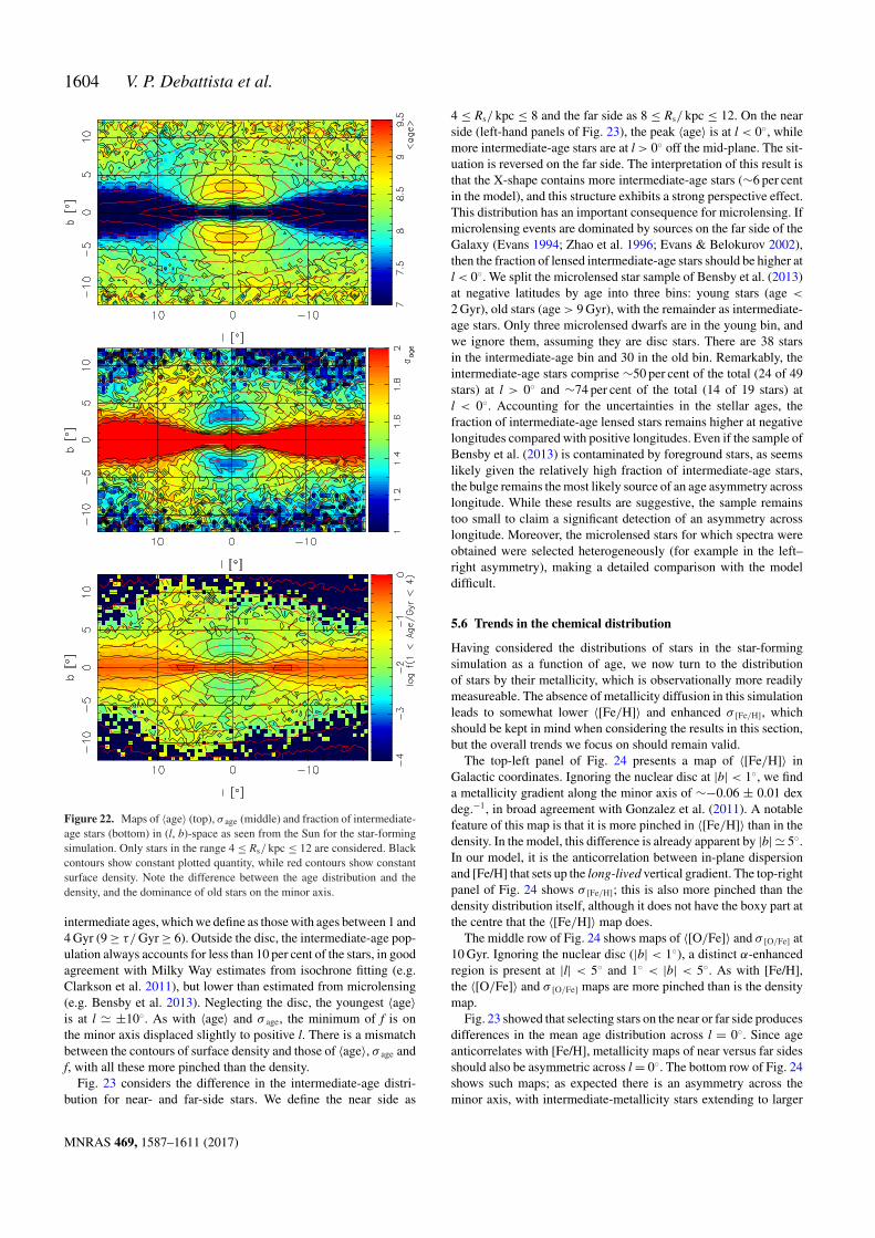
Fig. 22 shows the average age, ⟨age⟩, (top panel) and the standarddeviation in the age, σ age, (middle panel) in (l, b)-space. The peakof ⟨age⟩ is on the minor axis, although a small shift to positive l dueto the effect of perspective is evident. At the same location, σ age isat a minimum. The peak in ⟨age⟩ and the minimum in σ age are dueto the fact that it is the oldest stars that ascend the furthest on thebar’s minor axis, giving rise to a vertical age gradient and a mini-mum in σ age as seen from the Sun. Younger populations are insteadmore peanut-shaped. The dominance of the oldest stars above themid-plane is consistent with observations in the Milky Way (e.g.Ortolani et al. 1995; Kuijken & Rich 2002; Zoccali et al. 2003;Sahu et al. 2006; Clarkson et al. 2008, 2011; Brown et al. 2010;Valenti et al. 2013). Ness et al. (2014) showed that, none the less,younger stars are also mixed in with the old stars, particularly whenthe most metal-rich populations are considered, even at latitudes|b| ≥ 2◦. This qualitatively agrees with the finding of younger mi-crolensed dwarf stars (Bensby et al. 2011, 2013). In the bottompanel of Fig. 22, we show the fraction, f, of all stars which have
MNRAS 469, 1587–1611 (2017)
1604 V. P. Debattista et al.
Figure 22. Maps of ⟨age⟩ (top), σ age (middle) and fraction of intermediate-age stars (bottom) in (l, b)-space as seen from the Sun for the star-formingsimulation. Only stars in the range 4 ≤ Rs/ kpc ≤ 12 are considered. Blackcontours show constant plotted quantity, while red contours show constantsurface density. Note the difference between the age distribution and thedensity, and the dominance of old stars on the minor axis.
intermediate ages, which we define as those with ages between 1 and4 Gyr (9 ≥ τ/ Gyr ≥ 6). Outside the disc, the intermediate-age pop-ulation always accounts for less than 10 per cent of the stars, in goodagreement with Milky Way estimates from isochrone fitting (e.g.Clarkson et al. 2011), but lower than estimated from microlensing(e.g. Bensby et al. 2013). Neglecting the disc, the youngest ⟨age⟩is at l ≃ ±10◦. As with ⟨age⟩ and σ age, the minimum of f is onthe minor axis displaced slightly to positive l. There is a mismatchbetween the contours of surface density and those of ⟨age⟩, σ age andf, with all these more pinched than the density.
Fig. 23 considers the difference in the intermediate-age distri-bution for near- and far-side stars. We define the near side as
4 ≤ Rs/ kpc ≤ 8 and the far side as 8 ≤ Rs/ kpc ≤ 12. On the nearside (left-hand panels of Fig. 23), the peak ⟨age⟩ is at l < 0◦, whilemore intermediate-age stars are at l > 0◦ off the mid-plane. The sit-uation is reversed on the far side. The interpretation of this result isthat the X-shape contains more intermediate-age stars (∼6 per centin the model), and this structure exhibits a strong perspective effect.This distribution has an important consequence for microlensing. Ifmicrolensing events are dominated by sources on the far side of theGalaxy (Evans 1994; Zhao et al. 1996; Evans & Belokurov 2002),then the fraction of lensed intermediate-age stars should be higher atl < 0◦. We split the microlensed star sample of Bensby et al. (2013)at negative latitudes by age into three bins: young stars (age <
2 Gyr), old stars (age > 9 Gyr), with the remainder as intermediate-age stars. Only three microlensed dwarfs are in the young bin, andwe ignore them, assuming they are disc stars. There are 38 starsin the intermediate-age bin and 30 in the old bin. Remarkably, theintermediate-age stars comprise ∼50 per cent of the total (24 of 49stars) at l > 0◦ and ∼74 per cent of the total (14 of 19 stars) atl < 0◦. Accounting for the uncertainties in the stellar ages, thefraction of intermediate-age lensed stars remains higher at negativelongitudes compared with positive longitudes. Even if the sample ofBensby et al. (2013) is contaminated by foreground stars, as seemslikely given the relatively high fraction of intermediate-age stars,the bulge remains the most likely source of an age asymmetry acrosslongitude. While these results are suggestive, the sample remainstoo small to claim a significant detection of an asymmetry acrosslongitude. Moreover, the microlensed stars for which spectra wereobtained were selected heterogeneously (for example in the left–right asymmetry), making a detailed comparison with the modeldifficult.
5.6 Trends in the chemical distribution
Having considered the distributions of stars in the star-formingsimulation as a function of age, we now turn to the distributionof stars by their metallicity, which is observationally more readilymeasureable. The absence of metallicity diffusion in this simulationleads to somewhat lower ⟨[Fe/H]⟩ and enhanced σ [Fe/H], whichshould be kept in mind when considering the results in this section,but the overall trends we focus on should remain valid.
The top-left panel of Fig. 24 presents a map of ⟨[Fe/H]⟩ inGalactic coordinates. Ignoring the nuclear disc at |b| < 1◦, we finda metallicity gradient along the minor axis of ∼−0.06 ± 0.01 dexdeg.−1, in broad agreement with Gonzalez et al. (2011). A notablefeature of this map is that it is more pinched in ⟨[Fe/H]⟩ than in thedensity. In the model, this difference is already apparent by |b| ≃ 5◦.In our model, it is the anticorrelation between in-plane dispersionand [Fe/H] that sets up the long-lived vertical gradient. The top-rightpanel of Fig. 24 shows σ [Fe/H]; this is also more pinched than thedensity distribution itself, although it does not have the boxy part atthe centre that the ⟨[Fe/H]⟩ map does.
The middle row of Fig. 24 shows maps of ⟨[O/Fe]⟩ and σ [O/Fe] at10 Gyr. Ignoring the nuclear disc (|b| < 1◦), a distinct α-enhancedregion is present at |l| < 5◦ and 1◦ < |b| < 5◦. As with [Fe/H],the ⟨[O/Fe]⟩ and σ [O/Fe] maps are more pinched than is the densitymap.
Fig. 23 showed that selecting stars on the near or far side producesdifferences in the mean age distribution across l = 0◦. Since ageanticorrelates with [Fe/H], metallicity maps of near versus far sidesshould also be asymmetric across l = 0◦. The bottom row of Fig. 24shows such maps; as expected there is an asymmetry across theminor axis, with intermediate-metallicity stars extending to larger
MNRAS 469, 1587–1611 (2017)

Kinematic fractionation by an evolving bar 1605
Figure 23. Near- versus far-side stellar age distributions in the star-forming simulation. Top row: maps of ⟨age⟩. Bottom row: maps of fraction of intermediate-age (1 Gyr ≤ age ≤ 4 Gyr) stars. The maps on the left are for near-side stars (4 ≤ Rs/ kpc ≤ 8), while those on the right are for the far-side stars (8 ≤ Rs/ kpc≤ 12). Black contours show constant plotted quantity while red contours show constant surface density of the population under consideration. Away from theminor axis younger stars contribute most on the side where the arms of the X-shape are located. Thus, the greater vertical extent of the intermediate-age starsis at l > 0◦, a perspective effect.
latitude at l > 0◦ on the near side and at l < 0◦ on the far side.However, this difference is not as prominent as in the ages. As withages, this asymmetry will manifest in microlensed stars. Using themicrolensing data of Bensby et al. (2013), we find that there is ahigher average metallicity for lensed stars at l < 0◦ than at l > 0◦,but again the number of stars is too small for this result to be verysignificant.
Ness et al. (2013a) showed that, in the ARGOS survey, the frac-tion of metal-rich (their component A) stars decreases with latitude.In contrast, the fraction of metal-poor stars (their component C) in-creases relative to the intermediate-metallicity stars although theyremain less abundant. Fig. 25 shows maps of the fraction of stars inthe same three broad metallicity bins A, B and C as in Ness et al.(2013a, we stress that these are only convenient bins, not distinctstructural components). The metal-rich population A is dominantat low latitudes, but drops off rapidly with increasingly latitude,as found also by Ness et al. (2013a). The metal-poor population Cinstead follows the opposite trend, representing a smaller popula-tion at low latitudes, but increases with latitude. The intermediate-metallicity population B dominates everywhere except near the discwhere population A dominates. These are all trends that are in agree-ment with the findings of Ness et al. (2013a).
Recently, Zoccali et al. (2017) parametrized the metallicity distri-bution in each of the 26 fields of the GIBS survey into a metal-poorand a metal-rich components. They presented a density map for each
of the two components for −10◦ < l < 10◦ and −10◦ < b < 10◦
showing that the metal-poor population is more centrally concen-trated than the metal-rich one, and has a more axisymmetric spatialdistribution. On the other hand, the metal-rich population has abox-like distribution. These trends are consistent with the results ofFig. 25.
6 D ISCUSSION
The separation by the bar of different stellar populations onthe basis of their in-plane kinematics presents a novel expla-nation for the origin of many of the trends seen in the MilkyWay’s bulge, which have seemed to require more than one for-mation mechanism. Because this mechanism has never been de-scribed before, we coin the term ‘kinematic fractionation’ to referto it.
Kinematic fractionation circumvents the need for two or morecomponents to explain the trends observed in the bulge by employ-ing a continuum of stellar populations with different in-plane ran-dom motions, a very natural outcome of internal evolution. Heatingcan be accomplished in a variety of ways, including star-formingclumps, spirals, lopsidedness and other perturbations, supernovafeedback, gas turbulence and even interactions, but there is noneed to generate a separate population (a thick disc or a classical
MNRAS 469, 1587–1611 (2017)

1606 V. P. Debattista et al.
Figure 24. The stellar chemistry in the star-forming simulation. Top: maps of ⟨[Fe/H]⟩ (left) and σ [Fe/H] (right) in (l, b)-space as seen from the Sun. Onlystars in the range 4 ≤ Rs/ kpc ≤ 12 are considered. Middle: same as top row for [O/Fe]. Bottom: maps of ⟨[Fe/H]⟩ for near-side (left) and far-side (right)stars. Black contours show constant plotted quantity, while red contours show constant surface density of the population under consideration. Note the verticalgradients in ⟨[Fe/H]⟩ and ⟨[O/Fe]⟩ and the mismatch between density and chemistry contours.
accreted bulge) in the process. Moreover, early discs may form hot-ter directly (e.g. Bird et al. 2013). As we showed in the star-formingsimulation, at early times even 2 Gyr is enough time to produce asignificant difference in the random motions between younger andolder stars, and in the Milky Way the bar may have required evenlonger to form. Nor do the trends observed in the Milky Way re-quire that different spatial regions of the disc contribute to differentparts of the bulge. For instance, one of the key differences betweenour model and earlier work is that the vertical metallicity gradientresults not from a radial gradient in the initial system, but from
the correlation between age (and metallicity) and kinematics at barformation. This results in a long-lived vertical gradient.
The star-forming simulation we have compared the Milky Wayto is not a particularly good match to it. Thus, the results presentedhere have focused on trends, not on detailed matches to observations.On the other hand, the very fact that this quite generic model pro-duces trends that are also seen in the Milky Way argues very force-fully that the model captures the essential physics that producesthese non-trivial trends, unless we are prepared to accept a quiteremarkable coincidence.
MNRAS 469, 1587–1611 (2017)
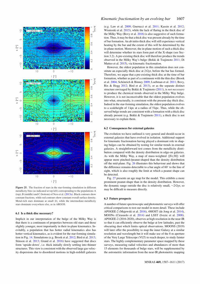
Kinematic fractionation by an evolving bar 1607
Figure 25. The fraction of stars in the star-forming simulation in differentmetallicity bins (as indicated at top left) corresponding to the populations A(top), B (middle) and C (bottom) of Ness et al. (2013a). Black contours showconstant fractions, while red contours show constant overall surface density.Metal-rich stars dominate at small |b|, while the intermediate-metallicitystars dominate everywhere else, as in ARGOS.
6.1 Is a thick disc necessary?
Implicit in our interpretation of the bulge of the Milky Way isthat there is a continuum of properties between old stars and thoseslightly younger, most importantly in their in-plane kinematics. In-evitably, a population that has hotter radial kinematics also hashotter vertical kinematics, as is evident for the star-forming simula-tion in Fig. 14. Simulations (e.g. Brook et al. 2012; Bird et al. 2013;Stinson et al. 2013; Grand et al. 2016) have suggested that discsform ‘upside-down’, i.e. thick initially slowly settling into thinnerstructures. This view is consistent with the observed large gas veloc-ity dispersions due to disordered motions in high-redshift galaxies
(e.g. Law et al. 2009; Gnerucci et al. 2011; Kassin et al. 2012;Wisnioski et al. 2015), while the lack of flaring in the thick disc ofthe Milky Way (Bovy et al. 2016) is also suggestive of such forma-tion. Thus, it may be that a thick disc was present already by the timeof bar formation. An ab initio thick disc will still experience verticalheating by the bar and the extent of this will be determined by thein-plane motion. Moreover, the in-plane motion of such a thick discwill determine whether its stars form part of the X-shape (see Sec-tion 3.2). A pre-existing thick disc will therefore produce the trendsobserved in the Milky Way’s bulge (Bekki & Tsujimoto 2011; DiMatteo et al. 2015), via kinematic fractionation.
However, the oldest population in this simulation does not con-stitute an especially thick disc at 2 Gyr, before the bar has formed.Therefore, we argue that a pre-existing thick disc at the time of barformation, whether as part of a continuum with the thin disc (Brooket al. 2004; Schonrich & Binney 2009; Loebman et al. 2011; Bovy,Rix & Hogg 2012; Bird et al. 2013), or as the separate distinctstructure envisaged by Bekki & Tsujimoto (2011), is not necessaryto produce the chemical trends observed in the Milky Way bulge.However, it is not inconceivable that the oldest population evolvesinto what, structurally, is consistent with the present-day thick disc.Indeed in the star-forming simulation, the oldest population evolvesto a scaleheight of 1 kpc at a radius of 5 kpc. Thus, while the ob-served bulge trends are consistent with a formation with a thick discalready present (e.g. Bekki & Tsujimoto 2011), a thick disc is notnecessary to explain them.
6.2 Consequences for external galaxies
The evolution we have outlined is very general and should occur inexternal galaxies that have evolved in isolation. Additional supportfor kinematic fractionation having played a dominant role in shap-ing bulges can be obtained by testing for similar trends in externalgalaxies. A straightforward test comes from the metallicity distri-bution compared with the density distribution in edge-on galaxies.As with the Milky Way, a map of mass-weighted ⟨[Fe/H]⟩ willappear more pinched-/peanut-shaped than the density distributionoff the mid-plane. Fig. 26 illustrates this behaviour and shows thatthe difference remains detectable to a bar angle of 60◦ to the line ofsight, which is also roughly the limit at which a peanut shape canbe detected.
Fig. 27 presents an age map for the model. This exhibits a moreprominent peanut-shape than in the density distribution. However,the dynamic range outside the disc is relatively small, ∼2 Gyr, somay be difficult to measure directly.
6.3 Future prospects
A number of future spectroscopic and photometric surveys will offercritical comparisons to test our model in more detail. These includeAPOGEE-2 (Majewski et al. 2016), 4MOST (de Jong et al. 2014),MOONs (Cirasuolo et al. 2014) and LSST (Ivezic et al. 2008).APOGEE-2 (2016-2020), observes at high resolution in the near-IRso that it can efficiently observe the bulge at low latitudes, past theobscuring dust which limits optical observations. MOONS (2019)will later offer the possibility to map the inner Galaxy at a similarresolution and wavelength but it will make use of the 8 m apertureof the Very Large Telescope (VLT) to reach deeper, to study fainterstars. The highly complementary parameter space mapped by thesesurveys, measuring radial velocities and abundances of more than15 elements for thousands of bulge stars, will be supplemented bythe astrometric information from the near-IR photometric mapping
MNRAS 469, 1587–1611 (2017)

1608 V. P. Debattista et al.
Figure 26. Maps of ⟨[Fe/H]⟩ (black contours and colours) and surfacedensity (red contours) in the star-forming simulation seen edge-on withthe bar side-on (top), end-on (bottom) and two intermediate orientations(middle two panels). The bar’s orientation is indicated in the top right ofeach panel. These maps predict the trends in the metallicity distribution ofexternal B/P-bulge galaxies.
Figure 27. Map of ⟨age⟩ (black contours and colours) and surface density(red contours) in the star-forming simulation seen edge-on with the barside-on.
of the VVV survey. The kinematics, chemical abundances, propermotions and even spectroscopic age measurements of large numberof stars (Martig et al. 2015; Ness et al. 2016a), in addition to thoseof other Galactic components provided by optical surveys such asGaia, 4MOST, WEAVE and LSST, will provide the critical con-straints on our model, helping us understand the detailed formationhistory of the Galaxy. In this context, our model also presents thepossibility of defining optimal strategies during the planning stagesof forthcoming surveys.
Our predictions are general and not specific to the Milky Wayand so comparisons to boxy bulges in other spiral galaxies are alsovery important. Modern Integral Field Unit spectrographs and theirdedicated surveys offer a great opportunity for understanding thebulge of the Milky Way in context (Gonzalez & Gadotti 2016), bymeasuring the morphological aspects of other spiral galaxies andprevalence of mergers compared to secular evolution at high redshift(e.g. Gadotti et al. 2015).
Our results also point the way forward in terms of future effortsto simulate the Milky Way in detail. Since simulations with full gasphysics are subject to much more stochasticity, and are computa-tionally expensive, pure N-body simulations will continue to play animportant role in trying to understand the bulge of the Milky Way.Past pure N-body simulations of the Milky Way (e.g. Fux 1997;Shen et al. 2010; Martinez-Valpuesta & Gerhard 2011) have pro-duced good matches to the density distribution and kinematics of thebulge. Studying the age and metallicity distributions of such mod-els requires assigning to particles a population tag (age/chemistry)in some way. Martinez-Valpuesta & Gerhard (2013) used such atechnique to match the observed vertical [Fe/H] gradient; in theirapproach the metallicity of a particle was a function of its initialorbital radius. We propose that a more useful approach to assign-ing a population tag to particles is based on their initial orbitalcircularities, rather than on their initial position.
6.4 Summary
Our main conclusions can be summarized as follows
(i) Bars can efficiently separate disc stellar populations thatdiffer by their initial in-plane kinematics (see Section 3). Hotpopulations form bars with weak quadrupoles, become verticallythick, particularly at the centre, and are box-shaped, while the coolerpopulations host stronger bars, are thinner at the centre and thus pro-duce a peanut shape. We refer to this separation of populations askinematic fractionation.
(ii) The early rapid evolution of discs naturally imprints cor-relations (or anticorrelations) between age, σ R, [Fe/H] and [O/Fe],which leads to relations between σ R and chemistry (see Section 4.1).After bar formation, kinematic fractionation leads to different pop-ulations having different bar strengths, vertical distributions andB/P-bulge strengths, naturally without the need for a separate ori-gin for different populations. Instead the properties of the bulge varycontinuously with age. The underlying reason for these differencesis primarily the difference in the initial σ R and its strong dependenceon age in young galaxies (see Section 4.2).
(iii) Kinematic fractionation also leads to the X-shape that isstronger in relatively younger (metal-rich) stars than in the older(metal-poor) ones. In our star-forming model, a difference of just2 Gyr in age is sufficient to alter the final distribution of stars froma single peak to a bimodal distribution. This is also consistentwith observations in the Milky Way (Ness et al. 2012; Uttenthaleret al. 2012; Rojas-Arriagada et al. 2014). Moreover we predict that,
MNRAS 469, 1587–1611 (2017)

Kinematic fractionation by an evolving bar 1609
for tracers with small distance uncertainties, old populations willstill appear bimodal, while younger populations will be well sepa-rated (see Section 5.2).
(iv) Kinematic fractionation of a hot, older population and acooler, younger population produces a weaker old bar populationand a stronger young bar population, even if the difference in ageis only ∼2 Gyr. This is consistent with what is observed in theMilky Way, where the RR Lyrae trace a weak bar, while red clumpstars trace a stronger bar (Dekany et al. 2013). In addition, bulgeMira variables show a smooth variation from strongly barred tomore spheroidal distribution as a function of their age (Catchpoleet al. 2016, see Section 5.3).
(v) Comparing with the ARGOS data (Ness et al. 2013b), themodel is able to match the overall kinematics and those of themetal-rich population. Matching to the kinematics of the metal-poor population, with its relatively flat velocity dispersion whichvaries slowly with latitude, requires the addition of 15 per centof stars in a hot, slowly rotating component. This slowly rotat-ing population amounts to ∼5 per cent of all bulge stars. Assuminga bulge-to-total stellar mass ratio of ∼25 per cent (Bland-Hawthorn& Gerhard 2016), this amounts to 1.25 per cent of the stellar massof the Milky Way. We attribute these stars to a metal-poor halo,leaving no room for a classical bulge. This conclusion is in agree-ment with the independent result derived by Kormendy et al. (inprogress and private communication) that the Milky Way has noclassical bulge component: aside from the boxy bulge, near the cen-tre they find only a nuclear star cluster and a small discy pseudo-bulge. Bland-Hawthorn & Gerhard (2016) review some of the trendswhich have been used to argue for a bulge component built throughmergers (a ‘classical bulge’ component); we have shown here thatthese trends can be explained without such an accreted bulge (seeSection 5.4).
(vi) A vertically declining [Fe/H] gradient, and vertically rising[O/Fe] gradient, are established largely as a result of the differentvertical extents of different ages. A declining [Fe/H] gradient hasbeen found in the Milky Way (e.g. Zoccali et al. 2008; Gonza-lez et al. 2011; Johnson et al. 2013). Separating populations intobroad metallicity bins, as used in ARGOS (Ness et al. 2013a), weshowed that at low latitudes the metal-rich population dominateswith the low-metallicity and intermediate-metallicity bins provid-ing a smaller contribution. The contribution of the metal-rich pop-ulation drops rapidly at larger latitudes, with that of the low- andintermediate-metallicity bins rising. The intermediate-metallicitybin dominates at large latitudes. These trends are in agreement withobservations in the Milky Way (Ness et al. 2013a, see Section 5.6).
(vii) Because the minor axis is dominated by old, metal-poorstars, a prediction of the kinematic fractionation model is that theshape of the ⟨[Fe/H]⟩ (or ⟨[O/Fe]⟩ or ⟨age⟩) map in the (l, b)-planewill appear more pinched/peanut-shaped than the density distribu-tion. These trends will need to be verified in future surveys (seeSections 5.5 and 5.6).
(viii) We predict that microlensed dwarf stars on the far(Rs > 8 kpc) side of the Galaxy will contain more intermediate-age, metal-rich stars at negative longitudes compared with pos-itive longitudes. The data of Bensby et al. (2013) suggest suchtrends, but the number of spectroscopically measured microlenseddwarfs is still too small to confirm this result (see Sections 5.5and 5.6).
(ix) A simple test of the kinematic fractionation model is pro-vided by external edge-on barred galaxies with B/P bulges, forwhich maps of ⟨[Fe/H]⟩ will be more strongly pinched/peanut-shaped than the density distribution itself (see Section 6.2).
ACK NOW L E DG E ME NT S
VPD is supported by STFC Consolidated grant no. ST/M000877/1.MN is funded by the European Research Council under the Euro-pean Union’s Seventh Framework Programme (FP 7) ERC GrantAgreement no. 321035. MZ and DM acknowledge support by theMinistry of Economy, Development, and Tourism’s MillenniumScience Initiative through grant IC120009, awarded to The Millen-nium Institute of Astrophysics (MAS), by the BASAL-CATA Centerfor Astrophysics and Associated Technologies PFB-06, FondecytRegular Proyects 1130196 and 1150345 and (MZ) by CONICYT’sPCI grant DPI20140066. We acknowledge support from the ESFExchange Grant (number 4650) within the framework of the ESFActivity entitled ‘Gaia Research for European Astronomy Train-ing’. The star-forming simulation used in this paper was run at theHigh Performance Computing Facility of the University of CentralLancashire. The pure N-body simulations were run at the DiRACShared Memory Processing system at the University of Cambridge,operated by the COSMOS Project at the Department of AppliedMathematics and Theoretical Physics on behalf of the STFC DiRACHPC Facility (www.dirac.ac.uk). This equipment was funded byBIS National E-infrastructure capital grant ST/J005673/1, STFCcapital grant ST/H008586/1 and STFC DiRAC Operations grantST/K00333X/1. DiRAC is part of the National E-Infrastructure.We are deeply grateful to Larry Widrow for his support with usingGALACTICS, including providing us with a development version thatallows for two discs of different thickness. VPD acknowledges withgreat pleasure the support of the Pauli Center for Theoretical Stud-ies, which is supported by the Swiss National Science Foundation(SNF), the University of Zurich and ETH Zurich. He particularlythanks George Lake for arranging for his sabbatical visit duringwhich time this paper was completed. We thank Sandro Tacchella,Reynier Peletier, Peter Erwin and Marc Balcells for useful discus-sions. We thank the anonymous referee for useful comments thathave helped improve the paper.
R E F E R E N C E S
Alves D. R., 2000, ApJ, 539, 732Athanassoula E., 2002, ApJ, 569, L83Athanassoula E., 2005, MNRAS, 358, 1477Athanassoula E., Misiriotis A., 2002, MNRAS, 330, 35Aumer M., Binney J. J., 2009, MNRAS, 397, 1286Aumer M., Schonrich R., 2015, MNRAS, 454, 3166Babusiaux C., 2016, PASA, 33, e026Babusiaux C. et al., 2010, A&A, 519, A77Behroozi P. S., Wechsler R. H., Conroy C., 2013, ApJ, 770, 57Bekki K., Tsujimoto T., 2011, MNRAS, 416, L60Bensby T. et al., 2011, A&A, 533, A134Bensby T. et al., 2013, A&A, 549, A147Binney J., Tremaine S., 1987, Galactic Dynamics. Princeton Univ. Press,
Princeton, NJBinney J., Gerhard O. E., Stark A. A., Bally J., Uchida K. I., 1991, MNRAS,
252, 210Binney J., Gerhard O., Spergel D., 1997, MNRAS, 288, 365Bird J. C., Kazantzidis S., Weinberg D. H., Guedes J., Callegari S., Mayer
L., Madau P., 2013, ApJ, 773, 43Bland-Hawthorn J., Gerhard O., 2016, ARA&A, 54, 529Bovy J., Rix H.-W., Hogg D. W., 2012, ApJ, 751, 131Bovy J., Rix H.-W., Schlafly E. F., Nidever D. L., Holtzman J. A., Shetrone
M., Beers T. C., 2016, ApJ, 823, 30Brook C. B., Kawata D., Gibson B. K., Freeman K. C., 2004, ApJ, 612, 894Brook C. B. et al., 2012, MNRAS, 426, 690Brown T. M. et al., 2010, ApJ, 725, L19
MNRAS 469, 1587–1611 (2017)

1610 V. P. Debattista et al.
Bureau M., Athanassoula E., 2005, ApJ, 626, 159Calamida A. et al., 2014, ApJ, 790, 164Casagrande L., Schonrich R., Asplund M., Cassisi S., Ramırez I., Melendez
J., Bensby T., Feltzing S., 2011, A&A, 530, A138Catchpole R. M., Whitelock P. A., Feast M. W., Hughes S. M. G., Irwin M.,
Alard C., 2016, MNRAS, 455, 2216Cirasuolo M. et al., 2014, in Ramsay S. K., McLean I. S., Takami H., eds,
Proc. SPIE Conf. Ser., Vol. 9147, Ground-based and Airborne Instru-mentation for Astronomy V. SPIE, Bellingham, p. 91470N
Clarkson W. et al., 2008, ApJ, 684, 1110Clarkson W. I. et al., 2011, ApJ, 735, 37Cohen R. J., Few R. W., 1976, MNRAS, 176, 495Cole D. R., Debattista V. P., Erwin P., Earp S. W. F., Roskar R., 2014,
MNRAS, 445, 3352Combes F., Sanders R. H., 1981, A&A, 96, 164Combes F., Debbasch F., Friedli D., Pfenniger D., 1990, A&A, 233, 82de Jong R. S. et al., 2014, in Ramsay S. K., McLean I. S., Takami H., eds,
Proc. SPIE Conf. Ser., Vol. 9147, Ground-based and Airborne Instru-mentation for Astronomy V. SPIE, Bellingham, p. 91470M
de Vaucouleurs G., 1964, in Kerr F. J., ed., IAU Symp., Vol. 20, The Galaxyand the Magellanic Clouds. Kluwer, Dordrecht, p. 195
Debattista V. P., Sellwood J. A., 1998, ApJ, 493, L5Debattista V. P., Sellwood J. A., 2000, ApJ, 543, 704Debattista V. P., Carollo C. M., Mayer L., Moore B., 2005, ApJ, 628,
678Debattista V. P., Mayer L., Carollo C. M., Moore B., Wadsley J., Quinn T.,
2006, ApJ, 645, 209Debattista V. P., Ness M., Earp S. W. F., Cole D. R., 2015, ApJ, 812, L16Dekany I., Minniti D., Catelan M., Zoccali M., Saito R. K., Hempel M.,
Gonzalez O. A., 2013, ApJ, 776, L19Di Matteo P. et al., 2014, A&A, 567, A122Di Matteo P. et al., 2015, A&A, 577, A1Dwek E. et al., 1995, ApJ, 445, 716Erwin P., Beltran J. C. V., Graham A. W., Beckman J. E., 2003, ApJ, 597,
929Erwin P. et al., 2015, MNRAS, 446, 4039Evans N. W., 1994, ApJ, 437, L31Evans N. W., Belokurov V., 2002, ApJ, 567, L119Ferreras I., Wyse R. F. G., Silk J., 2003, MNRAS, 345, 1381Fisher D. B., Drory N., 2016, in Laurikainen E., Peletier R., Gadotti D.,
eds, Astrophysics and Space Science Library, Vol. 418, Galactic Bulges.Springer-Verlag, Switzerland, p. 41
Fux R., 1997, A&A, 327, 983Fux R., 1999, A&A, 345, 787Gadotti D. A., Seidel M. K., Sanchez-Blazquez P., Falcon-Barroso J.,
Husemann B., Coelho P., Perez I., 2015, A&A, 584, A90Gardner E., Debattista V. P., Robin A. C., Vasquez S., Zoccali M., 2014,
MNRAS, 438, 3275Gerhard O., Martinez-Valpuesta I., 2012, ApJ, 744, L8Gerhard O. E., Vietri M., 1986, MNRAS, 223, 377Glazebrook K., 2013, PASA, 30, e056Gnerucci A. et al., 2011, A&A, 528, A88Gonzalez O. A., Gadotti D., 2016, in Laurikainen E., Peletier
R., Gadotti D., eds, Astrophysics and Space ScienceLibrary, Vol. 418, Galactic Bulges. Springer-Verlag, Switzerland,p. 199
Gonzalez O. A. et al., 2011, A&A, 530, A54Gonzalez O. A., Rejkuba M., Zoccali M., Valenti E., Minniti D., Schultheis
M., Tobar R., Chen B., 2012, A&A, 543, A13Gonzalez O. A., Zoccali M., Debattista V. P., Alonso-Garcıa J., Valenti E.,
Minniti D., 2015, A&A, 583, L5Grand R. J. J., Springel V., Gomez F. A., Marinacci F., Pakmor R., Campbell
D. J. R., Jenkins A., 2016, MNRAS, 459, 199Grieco V., Matteucci F., Pipino A., Cescutti G., 2012, A&A, 548, A60Guedes J., Mayer L., Carollo M., Madau P., 2013, ApJ, 772, 36Hammersley P. L., Garzon F., Mahoney T. J., Lopez-Corredoira M., Torres
M. A. P., 2000, MNRAS, 317, L45Hill V. et al., 2011, A&A, 534, A80
Holmberg J., Nordstrom B., Andersen J., 2009, A&A, 501, 941House E. L. et al., 2011, MNRAS, 415, 2652Howard C. D., Rich R. M., Reitzel D. B., Koch A., De Propris R., Zhao H.,
2008, ApJ, 688, 1060Ivezic Z. et al., 2008, preprint (arXiv:0805.2366)Johnson C. I., Rich R. M., Fulbright J. P., Valenti E., McWilliam A., 2011,
ApJ, 732, 108Johnson C. I., Rich R. M., Kobayashi C., Kunder A., Pilachowski C. A.,
Koch A., de Propris R., 2013, ApJ, 765, 157Juric M. et al., 2008, ApJ, 673, 864Kassin S. A. et al., 2012, ApJ, 758, 106Kauffmann G., White S. D. M., Guiderdoni B., 1993, MNRAS, 264, 201Kennicutt R. C. Jr., Tamblyn P., Congdon C. E., 1994, ApJ, 435, 22Kormendy J., Kennicutt R. C., 2004, ARA&A, 42, 603Kuijken K., Dubinski J., 1995, MNRAS, 277, 1341Kuijken K., Rich R. M., 2002, AJ, 124, 2054Kunder A. et al., 2012, AJ, 143, 57Kunder A. et al., 2016, ApJ, 821, L25Law D. R., Steidel C. C., Erb D. K., Larkin J. E., Pettini M., Shapley A. E.,
Wright S. A., 2009, ApJ, 697, 2057Li Z., Gerhard O., Shen J., Portail M., Wegg C., 2016, ApJ, 824, 13Li Z.-Y., Shen J., 2012, ApJ, 757, L7Li Z.-Y., Shen J., 2015, ApJ, 815, L20Liszt H. S., Burton W. B., 1980, ApJ, 236, 779Loebman S. R., Roskar R., Debattista V. P., Ivezic, Z., Quinn T. R., Wadsley
J., 2011, ApJ, 737, 8Loebman S. R., Debattista V. P., Nidever D. L., Hayden M. R., Holtzman J.
A., Clarke A. J., Roskar R., Valluri M., 2016, ApJ, 818, L6Majewski S. R. et al., 2016, Astron. Nachr., 337, 863Martig M. et al., 2015, MNRAS, 451, 2230Martinez-Valpuesta I., Gerhard O., 2011, ApJ, 734, L20Martinez-Valpuesta I., Gerhard O., 2013, ApJ, 766, L3Martinez-Valpuesta I., Shlosman I., Heller C., 2006, ApJ, 637, 214McWilliam A., Zoccali M., 2010, ApJ, 724, 1491Mendez-Abreu J., Debattista V. P., Corsini E. M., Aguerri J. A. L., 2014,
A&A, 572, A25Merritt D., Sellwood J. A., 1994, ApJ, 425, 551Minniti D. et al., 2010, New Astron., 15, 433Mulder W. A., Liem B. T., 1986, A&A, 157, 148Nakada Y., Onaka T., Yamamura I., Deguchi S., Hashimoto O., Izumiura
H., Sekiguchi K., 1991, Nature, 353, 140Nataf D. M., Udalski A., Gould A., Fouque P., Stanek K. Z., 2010, ApJ,
721, L28Navarro J. F., Frenk C. S., White S. D. M., 1996, ApJ, 462, 563Ness M. et al., 2012, ApJ, 756, 22Ness M. et al., 2013a, MNRAS, 430, 836Ness M. et al., 2013b, MNRAS, 432, 2092Ness M., Debattista V. P., Bensby T., Feltzing S., Roskar R., Cole D. R.,
Johnson J. A., Freeman K., 2014, ApJ, 787, L19Ness M., Hogg D. W., Rix H.-W., Martig M., Pinsonneault M. H., Ho A. Y.
Q., 2016a, ApJ, 823, 114Ness M. et al., 2016b, ApJ, 819, 2Nidever D. L. et al., 2012, ApJ, 755, L25Nikolaev S., Weinberg M. D., 1997, ApJ, 487, 885Nordstrom B. et al., 2004, A&A, 418, 989O’Neill J. K., Dubinski J., 2003, MNRAS, 346, 251Ortolani S., Renzini A., Gilmozzi R., Marconi G., Barbuy B., Bica E., Rich
R. M., 1995, Nature, 377, 701Paczynski B., Stanek K. Z., Udalski A., Szymanski M., Kaluzny J., Kubiak
M., Mateo M., Krzeminski W., 1994, ApJ, 435, L113Patel S. G. et al., 2013, ApJ, 778, 115Peters W. L., III, 1975, ApJ, 195, 617Quillen A. C., 2002, AJ, 124, 722Quillen A. C., Minchev I., Sharma S., Qin Y.-J., Di Matteo P., 2014, MNRAS,
437, 1284Raha N., Sellwood J. A., James R. A., Kahn F. D., 1991, Nature, 352, 411Raiteri C. M., Villata M., Navarro J. F., 1996, A&A, 315, 105Rojas-Arriagada A. et al., 2014, A&A, 569, A103
MNRAS 469, 1587–1611 (2017)

Kinematic fractionation by an evolving bar 1611
Saha K., Gerhard O., 2013, MNRAS, 430, 2039Saha K., Martinez-Valpuesta I., Gerhard O., 2012, MNRAS, 421, 333Sahu K. C. et al., 2006, Nature, 443, 534Saito R. K., Zoccali M., McWilliam A., Minniti D., Gonzalez O. A., Hill V.,
2011, AJ, 142, 76Samland M., 2002, Ap&SS, 281, 305Schonrich R., Binney J., 2009, MNRAS, 399, 1145Sellwood J. A., 1983, J. Comput. Phys., 50, 337Sellwood J. A., 1985, MNRAS, 217, 127Sevenster M. N., 1996, in Buta R., Crocker D. A., Elmegreen B. G., eds,
ASP Conf. Ser. Vol. 91, IAU Colloq. 157: Barred Galaxies. Astron. Soc.Pac., San Francisco, p. 536
Shen J., Rich R. M., Kormendy J., Howard C. D., De Propris R., Kunder A.,2010, ApJ, 720, L72
Stadel J. G., 2001, PhD thesis, Univ. WashingtonStanek K. Z., Mateo M., Udalski A., Szymanski M., Kaluzny J., Kubiak M.,
1994, ApJ, 429, L73Stanek K. Z., Udalski A., Szymanski M., Kaluzny J., Kubiak M., Mateo M.,
Krzeminski W., 1997, ApJ, 477, 163Stinson G. S. et al., 2013, MNRAS, 436, 625Tacchella S. et al., 2015, Science, 348, 314Terrazas B. A., Bell E. F., Henriques B. M. B., White S. D. M., 2016,
MNRAS, 459, 1929Thielemann F.-K., Nomoto K., Yokoi K., 1986, A&A, 158, 17Uttenthaler S., Schultheis M., Nataf D. M., Robin A. C., Lebzelter T., Chen
B., 2012, A&A, 546, A57Valenti E., Zoccali M., Renzini A., Brown T. M., Gonzalez O. A., Minniti
D., Debattista V. P., Mayer L., 2013, A&A, 559, A98van Dokkum P. G. et al., 2013, ApJ, 771, L35Wadsley J. W., Stadel J., Quinn T., 2004, New Astron., 9, 137Walker A. R., 1989, PASP, 101, 570Wegg C., Gerhard O., 2013, MNRAS, 435, 1874Wegg C., Gerhard O., Portail M., 2015, MNRAS, 450, 4050Weidemann V., 1987, A&A, 188, 74Weiland J. L. et al., 1994, ApJ, 425, L81Weinberg M. D., 1985, MNRAS, 213, 451Whitelock P., Catchpole R., 1992, in Blitz L., ed., Astrophysics and Space
Science Library, Vol. 180, The Center, Bulge, and Disk of the MilkyWay. Springer-Verlag, Dordrecht, Netherlands, p. 103
Widrow L. M., Dubinski J., 2005, ApJ, 631, 838Widrow L. M., Pym B., Dubinski J., 2008, ApJ, 679, 1239Wielen R., 1977, A&A, 60, 263Wisnioski E. et al., 2015, ApJ, 799, 209Wyatt S. P., Cahn J. H., 1983, ApJ, 275, 225Zhao H., Rich R. M., Spergel D. N., 1996, MNRAS, 282, 175Zoccali M. et al., 2003, A&A, 399, 931Zoccali M., Hill V., Lecureur A., Barbuy B., Renzini A., Minniti D., Gomez
A., Ortolani S., 2008, A&A, 486, 177Zoccali M. et al., 2014, A&A, 562, A66Zoccali M. et al., 2017, A&A, 599, A12
A P P E N D I X A : H E I G H T D E P E N D E N C E O FO R B I TA L F R E QU E N C I E S
Here, we demonstrate that the vertical frequency, ν, of a star declinesmore rapidly with increasing maximum height, zmax, than does theorbital frequency, #. We do this directly by computing orbits ofstars in the pure N-body model with disc D5 described in Section 3.We select all stars in a narrow annulus of guiding radius 3.95 ≤Rgui/ kpc ≤ 4.05, where Rgui = Jz/Vc, Jz is the angular momentumof the particle about the z-axis, and Vc is the circular velocity at
Figure A1. Filled triangles show ν/2, while filled circles show # for indi-vidual star particles. Black, red and blue points show increasing eccentricityas indicated. All orbits have guiding radius 3.95 ≤ Rgui/ kpc ≤ 4.05.
this radius. We choose this annulus because the peanut shape isvery distinct at the end of the simulation in this region; howeverthe vertical distribution of the stars is much narrower than the finalpeanut shape. We integrate orbits for ∼9000 of these particles, usinga time-step of 104 yr, saving the phase space coordinates of eachstar every time-step over a 1 Gyr period. From these orbits, we thencompute the eccentricity of the orbit
ϵ = Rmax − Rmin
Rmax + Rmin(A1)
where Rmax and Rmin are the maximum and minimum radius reached;ϵ = 0 corresponds to a circular orbit. We also compute zmax as wellas the tangential and vertical frequencies, # and ν, respectively.
Fig. A1shows the result of this calculation. It is very clear thatν/2 declines much more rapidly with zmax than does #, which onlychanges by ∼3 Gyr−1 over this vertical range. The figure also showsthe variation of # and ν/2 as a function of ϵ. The angular frequency# decreases with increasing ϵ, while the change in ν/2 with ϵ ismore modest.
This paper has been typeset from a TEX/LATEX file prepared by the author.
MNRAS 469, 1587–1611 (2017)