september 2000 update - the national...

Economic modelsat the Bank of England

September 2000 update

Bank of England

Any enquiries about this publication should be addressed to:

Meghan QuinnMonetary AnalysisTelephone 020-7601 5269Fax 020-7601 5196email: [email protected]

Further copies of this publication are available from:

Publications GroupTelephone 020-7601 4030Fax 020-7601 3298email: [email protected]

The Bank’s Internet pages are at http://www.bankofengland.co.uk

Bank of England, Threadneedle Street, London, EC2R 8AH.

Printed by Park Communications Ltd© Bank of England 2000ISBN 1 85730 182 X

Contents Page

1 Introduction 51.1 Models, policy analysis and forecasting 51.2 General characteristics of the macroeconometric model 61.3 Changes to the MM 71.4 Other models added to the suite 8

2 Overview of the macroeconometric model 9

3 The structure of the macroeconometric model 103.1 The long-run real growth path 103.2 The long-run nominal growth path and inflation 133.3 Short-run dynamics and inflation 14

4 Recent changes to the model specification 15

5 Simulation properties 165.1 Rationale for simulations 165.2 Temporary interest rate shock 175.3 Exogenous change in a price level target 18

6 Detailed equation listing 206.1 Money, financial and wealth variables 216.2 Demand and output 276.3 Labour market 366.4 Prices 426.5 Fiscal policy 546.6 Income 56

7 Variables listing 59

Bibliography 68

The macroeconometric model 5

1 Introduction

In April 1999, the Bank of England published Economic Models at the Bank of England, settingout the economic modelling tools that help the Monetary Policy Committee (MPC) in its work.That volume included a complete listing of the Bank’s main macroeconometric model (MM), andoutlined the other members of the suite of models used for various aspects of monetary policyanalysis. It was made clear at the time that neither the MM nor the other models in use should bethought of as fixed in form or content. Indeed, many aspects of the models are regularly reviewed,and new approaches to modelling aspects of the economy are continually investigated.

The purpose of this publication is to provide an update of the changes incorporated in the MMover the past 18 months. It provides a written listing of the MM, to accompany the simultaneousrelease of the model code in electronic form. At the same time, we reference some other workwithin the Bank that has added to the range of models in the suite and that is already publiclyavailable.

In this section we outline the Bank’s modelling philosophy (set out more fully in the earliervolume), describe the key features of the MM, highlight the main ways in which the MM haschanged since April 1999, and outline some other relevant modelling work. Sections 2 and 3explain the structure of the MM in more detail. Section 4 outlines the changes to the MM.Section 5 discusses the MM simulation properties. Finally, Sections 6 and 7 provide a completemodel listing, including diagnostics on estimated equations and data sources.

1.1 Models, policy analysis and forecasting

The MM is the main tool for producing projections of GDP growth and inflation shown in theInflation Report. The MM is built around a number of estimated econometric relationships, butsome of the model properties—notably the long-run properties—are imposed in the form ofparameter restrictions for theoretical consistency. There is a continual need to evaluate and updatevarious components of the MM. Estimated MM econometric relationships may have broken downor have changed in some way, so that research is required to investigate the causes and to testalternatives that may eventually be incorporated in the MM itself.

The Bank continues to use a range of models. Some provide inputs into the quarterly projections,while others are used to analyse specific policy questions that cannot be handled adequately withinthe MM. Some research may prove difficult or impossible to incorporate in the MM—forexample, it may involve a different level of aggregation. It would then be run in parallel toprovide a comparison with MM outputs, or to provide insights into aspects of the economy that theMM cannot address.

Occasionally, specific new policy issues arise that cannot be analysed using the existingframework, and models are set up specifically to examine the key features of the issue at hand.Examples have included the impact of the National Minimum Wage, the implementation of theWorking Time Directive, and the assessment of the impact on consumer spending of the windfalls

6 Economic models at the Bank of England

from building society demutualisations. In some cases, a purpose-built model may cease to be ofuse once the issue it addresses no longer has monetary policy significance. But in other cases thework is incorporated in tools that are used to assess issues of continuing relevance.

Each forecasting round requires assumptions to be made about a wide range of exogenousvariables. Auxiliary models are often used to inform these judgments. Some relate, for example,to the world economy or some element of it, such as commodity prices or the level of world trade.For the assessment of world economic activity and inflation, the MPC uses a model(1) of the worldeconomy provided by the National Institute of Economic and Social Research to help form itsjudgments. Other models relate to aspects of the domestic economy that are not formallymodelled in the MM, but where parameters may be varied or restricted as a result of the auxiliaryanalysis. In all cases, the assumptions incorporated in any specific forecast are a combination ofthose suggested by the auxiliary model and the application of the MPC’s judgment. Profit marginsand house prices are examples of areas where forecast assumptions are influenced by bothsupplementary modelling and MPC judgment.

Where the Bank does not have the tools to hand for analysing a specific issue, it will seek out thebest available analysis from the academic literature or from the research work of other centralbanks and research institutes. For this reason, Bank staff are encouraged to keep abreast of therelevant academic literature and to contribute to it by publication of working papers, contributionsto professional journals, and presenting their work at conferences. The Bank also runs a seminarseries, addressed both by outside experts and by internal staff. The general philosophy with whichthe Bank approaches modelling and forecasting in particular, and monetary policy analysis ingeneral, is one of pluralism and openness. We are happy to receive comments on this and on anyother publication, particularly suggestions on how things could be improved.

1.2 General characteristics of the macroeconometric model

The core macroeconometric model (MM) consists of about 20 key equations determiningendogenous variables. There are a further 90 or so identities defining relationships betweenvariables, and there are about 30 exogenous variables whose paths have to be set, as discussedabove.

GDP is determined in the short term by the components of aggregate demand—privateconsumption, investment (including inventory investment), government consumption, and netexports.

In the longer term GDP is determined by supply-side factors, which determine potential output.Domestic firms are modelled as producing a single composite good using an aggregate productionfunction of the Cobb-Douglas form. So output is determined in the long run by the evolution ofthe capital stock, the labour supply and total factor productivity. These variables are assumed tobe unaffected by the price level or the inflation rate (so the model exhibits long-run monetaryneutrality and super-neutrality).

(1) The National Institute Global Economic Model (NiGEM).


Price level dynamics and the adjustment of actual output towards potential are broadly determinedby the interaction between aggregate demand and supply, augmented by explicit relationships foraspects of wage and price-setting. These relationships are consistent with the view that firms setdomestic output prices as a cyclically varying mark-up over unit labour costs. RPIY is determinedby an equation linking retail prices to domestic output prices and import prices. Firms are alsoassumed to determine the level of employment, and real wages are determined by bargaining in animperfectly competitive labour market. Inflation expectations have an explicit role in wagedetermination. But price responses are sluggish, so there is slow adjustment towards both real andnominal equilibria.

The appropriate assumptions under which to run the model depend on the exercise at hand. Forexample, short-run forecasting typically requires different assumptions from those used for long-run simulations, and for either purpose a wide range of alternative assumptions could bemade. For the main Inflation Report forecasts, nominal short-term interest rates are assumed to beconstant over the forecast period, but an alternative is also presented in which rates follow the pathimplied by market expectations. When using the MM for simulation purposes, the short rate canbe set according to a policy rule linking short-term nominal interest rates to the monetary policytarget, but the nature of this rule can take many different forms. Different exchange rateassumptions can be used in both the construction of projections and for simulations. A range ofpossible treatments is also available for the evolution of net financial wealth, and for inflationexpectations.

A further example of where different assumptions may be used for different purposes relates togovernment spending. The Inflation Report projections incorporate announced governmentspending plans, but some alternative assumption is needed in longer-term simulations, as spendingplans are not announced for more than a few years at a time. In this case, a common assumptionis that government consumption growth is fixed in either nominal or real terms. The properties ofthe model when used for simulation purposes are shown in Section 5 below.

1.3 Changes to the MM

The main areas of the MM in which changes have been introduced since April 1999 are:

● The consumption function now incorporates a new measure of labour income, whichincludes self-employment incomes (mixed incomes). Gross housing wealth and net financialwealth now have a separate role in the dynamics. And the real (short) interest rate matters inthe long run, while nominal short rates affect the dynamics.

● There is a new equation for house prices, which depend on average earnings and the longreal rate in the long run, while GDP enters the dynamics (in addition to earnings).

● Both export and import equations have been modified as a result of estimation on new data,the main effect being to lower slightly the relative price elasticities.


● RPIY is determined by a modified relationship that weights domestic and import prices.

In addition, there are other small modifications resulting from data revisions and definitionalchanges affecting the capital stock, investment, trade prices, earnings, employment, non-labourincome and the GDP deflator. There are minor changes to the treatment of value-added tax andspecial duties (affecting the link from RPIY to RPIX), and a new equation for the governmentexpenditure deflator has been introduced. These changes are discussed more fully in Section 4.The detailed specification of the current model is set out in Section 6.

The simulation properties of the MM, in terms of both timing and scale of responses, have notbeen affected substantially by the recent changes. For example, an unanticipated change in the short-term interest rate for four quarters still has its maximum impact on inflation after about ninequarters, and the order of magnitude is similar to that shown in the earlier publication. The currentMM suggests that unanticipated changes in interest rates have a slightly faster impact on real GDPthan the earlier version, with the peak impact being felt after four rather than five quarters. Thesize of the impact is comparable with the earlier version of the MM.

1.4 Other models added to the suite

There has been a large amount of work within the Bank of England over the past two yearsdesigned to throw light on specific monetary policy related issues. Some of this research feedsinto the background analysis prepared as input to the quarterly forecasting round, while other workfeeds into monthly briefings to highlight specific issues on an ad hoc basis. Specific examples canbe found in the papers published in the Bank’s working paper series. A selection of such researchis highlighted here.

● A series of papers has investigated the impact of model uncertainty on actual and optimalmonetary policy.(1)

● Further work using structural vector autoregressions has been done, following on fromresearch discussed in Chapter 5 of the 1999 volume. One example was aimed at identifyingmonetary policy shocks from the many other shocks that hit the economy, by imposing apriori restrictions.(2) Another example used related methods to investigate the empiricalrelationship between different measures of ‘gaps’ (output, employment and capacityutilisation) by the imposition of restrictions implied by economic theory.(3)

● Small-scale aggregated models (as discussed in Chapter 4 of the 1999 volume) have alsobeen used to investigate the relationship between optimal monetary policy and inflationprojections.(4)

(1) Hall, Salmon, Yates and Batini (1999); Martin and Salmon (1999); and Martin (1999).(2) Dhar, Pain and Thomas (2000).(3) Astley and Yates (1999). (This paper was mentioned in the April 1999 publication, but was published subsequently.)(4) Batini and Nelson (2000).


● Optimising models (of the type outlined in Chapter 6 of the 1999 volume) have been used toinvestigate several issues of relevance to monetary policy. For example, one model has beenused to investigate the determinants of the changing behaviour of mark-ups over time.(1)

Another paper has examined the potential impact of the labour market reforms of the 1980son the wage-setting and employment decisions of firms.(2)

● Further work has been done on the Phillips curve type models discussed in Chapter 3 of the1999 volume; this work may be published in due course.

● There has also been considerable work on developing tools for extracting and interpretinginformation from financial markets, for example about interest rate and inflationexpectations.(3)

For the remainder of this publication we focus entirely on the MM, how it has been developed andits properties.

2 Overview of the macroeconometric model

The macroeconometric model contains around 20 estimated econometric equations. These aresupplemented by identities, transformations and linking equations. Including exogenous variables,there are about 140 variables in the model database.(4)

The MM has three key features.

(i) A long-run growth path for real output, consistent with the following properties:

● price level neutrality: the long-run real growth path is independent of the price level. This isensured by restricting equations containing nominal variables to exhibit static homogeneity.

● inflation neutrality: the long-run real level of output and the unemployment rate areindependent of the inflation rate, ie the long-run Phillips curve is vertical. To ensure that thisholds, equations containing nominal variables are restricted to satisfy dynamic homogeneity,and inflation expectations are constrained to converge on actual inflation in the long run.

(ii) A long-run growth path for nominal (ie money-denominated) variables, determined by ananchor specified in terms of a target for a nominal variable (for example an inflation or aprice level target). This nominal anchor is usually secured by choosing a feedback rule formonetary policy linking the instrument of monetary policy (short-term nominal interestrates) to the selected target. Though the quantity of money does not have a causal role inthis set-up (over and above the inter-temporal price of money, ie interest rates) the money

(1) Britton, Larsen and Small (2000).(2) Millard (2000).(3) Anderson and Sleath (1999); Clews, Panigirtzoglou and Proudman (2000); and Bliss and Panigirtzoglou (2000).(4) See the variables listing in Section 7.


supply will move in line with nominal output in the long run, in the absence of persistentshifts in velocity.

(iii) Sluggish adjustment of nominal and real variables to economic shocks. Goods and labourmarkets are characterised by both real inertia (quantities take time to adjust to economicshocks) and nominal inertia (prices do not move immediately in response to changingeconomic conditions), which results in slow adjustment of the economy towards its long-rungrowth path. The speed of adjustment reflects the degree of inertia in the wage-price system,and the costs of adjusting employment or the capital stock.

3 The structure of the macroeconometric model

This section discusses the structure of the MM in more detail. We follow the three stagesdescribed above, by characterising the real and nominal long-run growth paths and the dynamicresponse of the economy when it is away from these paths. All variables are expressed in logs,unless otherwise stated.(1) Equation coefficients are written as Greek letters; for example interceptcoefficients are written as βz for the equation in which z is the dependent variable. A fulldescription of these and all the other model equations is given in Section 6.

3.1 The long-run real growth path

The core of the model’s supply side consists of four variables: output, labour (defined in terms ofhours worked), the capital stock (defined in terms of non-housing capital), and real wages.

Long-run output is determined by a simple Cobb-Douglas production function with constantreturns to scale and diminishing marginal returns to each factor of production, which can bewritten as:

y = βy + αµ T + α l + (1 – α)k (3.1.1)

where output (y) is produced by combinations of capital (k), labour (l) and labour-augmentingtechnical progress (µ T), which is assumed to be exogenous.(2)

Firms are assumed to choose labour and capital so as to maximise their profits. This implies thefollowing marginal revenue/product conditions with respect to labour and capital:

y – l = βl + w – pd (3.1.2)

y – k = βk + rc (3.1.3)

where w is the nominal wage, pd is the domestic product price (ie the GDP deflator), rc is the realcost of capital, and the long-run constants capture, among other things, the production technologyand the degree of competition in product and labour markets.

(1) The convention adopted throughout is for variables to be assigned upper-case and their logs to be assigned lower-case letters.(2) The parameter α is set at 0.7, consistent with the observed average share of income going to labour.


Equation (3.1.1) can be expressed as a labour demand equation as in (6.3.11) below by writingemployment on the left-hand side. Equation (3.1.2) can be expressed as either a labour demandcurve, by writing employment on the left-hand side, or as a price mark-up equation, with prices onthe left-hand side. In the equation listing in Section 6, it is expressed as a price mark-up over unitlabour costs (6.4.1). In the long run this mark-up is assumed constant. Together with theassumption of Cobb-Douglas technology this implies that long-run factor shares are also constant.Equation (3.1.3), expressed as the business investment equation (6.2.12), and the capitalaccumulation equation (6.2.11) together describe the investment/demand-for-capital relationship.

Wage-setting behaviour is consistent with an imperfectly competitive model of the labour market,where firms bargain with workers over real wages, but set goods prices and employment levels(see, for example, Layard, Nickell and Jackman (1991)). The real wage equation (3.1.4) which isestimated in equation (6.3.3) implies that, in the long run, real unit labour costs depend positivelyon a set of structural variables (Zs) (such as union power and the replacement ratio) and negativelyon the unemployment rate (U):(1)

w – pd = βw + y – l + θ1Zs – θ2U (3.1.4)

where the rate of unemployment is defined as the active working population minus employment asa proportion of the active working population by headcount (6.3.8). The link between employmentin terms of total hours worked and in terms of the number of people in work is given by arelationship for average hours (6.3.13).

Equation (3.1.2) and (3.1.4) both define alternative expressions for the labour share that must beconsistent in the long run. By substituting equation (3.1.2) into (3.1.4) and rearranging, the long-run unemployment rate (U*) can be expressed as:

U* = (βl + βw + θ1Zs) / θ2 (3.1.5)

In a closed economy, aggregate demand and supply cannot, by definition, diverge from each other.But in an open economy such as the United Kingdom, aggregate demand can be met fromoverseas as well as from domestic supply, and domestic supply can be sold overseas to meetforeign demand. So a stylised IS-curve model of aggregate demand can be written as:

yd = βyd+ γ1y + γ2yw + γ3r + γ4x (3.1.6)

where aggregate demand, yd, depends on domestic income (y), overseas income (yw), the realinterest rate (r) and the real exchange rate (x), which will affect the share of domestic and overseasdemand being spent on UK output.

(1) In all the supply-side equations, labour costs include employers’ taxes.


Summing the expenditure components of GDP determines aggregate demand:

● consumption (6.2.8) is modelled in the long run as a function of labour income, wealth andreal interest rates; nominal interest rates are included in the short-run dynamics to proxy forconfidence and cash-flow effects; and the change in unemployment is used to captureinfluences on precautionary saving;

● investment (6.2.11 and 6.2.12) is consistent with equation (3.1.3) above, and determines thestock of capital;

● stockbuilding (6.2.16 and 6.2.17) over the medium term is consistent with a downward trendin the long-run stock-output ratio;

● real government spending (6.2.15) is treated as exogenous in the simulations outlined inSection 5. But announced nominal government spending plans provide the basis forforecasting this component (with real government spending influenced by the projection forinflation);

● exports (6.2.18) depend on world trade volumes (weighted by UK market shares) and ameasure of the real exchange rate, which reflects the competitiveness of UK exports; and

● imports (6.2.19) are modelled as a function of domestic demand, a competitiveness term, anda proxy measure for the increase in gross trade flows relative to world demand arising fromincreased globalisation and international specialisation.

As the United Kingdom is an open economy, aggregate demand is brought into line with potentialsupply in the long run by movements in the real exchange rate, via a combination of changes inthe nominal exchange rate and domestic price level for a given path for foreign prices.

For simulation purposes, the nominal exchange rate (st) (6.1.6) is typically determined by theuncovered interest parity condition.(1) This relates expected changes in the exchange rate betweentwo currencies to differences in their interest rates and a risk premium. This can be written as:

st = set+1 + it – iwt – ρt (3.1.7)

where st is defined as the number of units of foreign currency per unit of domestic currency, se isthe expected value of the nominal exchange rate, i and iw are the domestic and foreign one-periodnominal interest rates respectively, and ρ is the risk premium. This relationship can be writtenequivalently as a relationship expressing the real exchange rate in terms of real interest rates:

xt = xet+1 + rt – rw

t – ρt (3.1.8)

(1) Since November 1999 the central projection in the Inflation Report has assumed that the nominal exchange rate evolves along a path halfwaybetween a constant rate and the path implied by the uncovered interest parity condition, conditioned on constant UK interest rates, with azero risk premium.


where rw is the world real interest rate. This implies that, in the long run, UK real interest rateswould differ from world real interest rates by the risk premium, if the long-run real exchange ratewere constant.

3.2 The long-run nominal growth path and inflation

The long-run levels of output and employment described above are independent of both the pricelevel and the rate of inflation. This reflects the theoretical presumption and empirical evidencethat there is no long-run trade-off between inflation and the level of output or employment.

The MM has several measures of prices:

● the domestic output price index (the GDP deflator at factor cost, pd) (6.4.1) is modelled as amark-up over unit labour costs, as described above;

● the RPIY price index (RPI excluding indirect and council taxes, and mortgage interestpayments) (6.4.5) is modelled as a weighted average of domestically consumed output pricesand import prices;

● RPIX (6.4.6) is then modelled by adding indirect and council taxes to RPIY;

● the retail price index (RPI) (6.4.11) is obtained by adding mortgage interest payments toRPIX;

● the consumers’ expenditure deflator (6.4.13) is assumed to grow in line with RPIX excludingcouncil taxes;

● the government consumption deflator (6.4.14) is assumed to grow in line with the average ofretail prices, excluding mortgage interest payments and council taxes, and unit labour costs;

● import prices (6.4.2) are assumed in the long run to be set by foreign suppliers in worldmarkets, with their sterling value determined by the nominal exchange rate; and

● export prices (6.4.3) reflect a weighted average of domestic costs, exchange rate adjustedworld prices, and oil prices.

The level and rate of change of the overall price level are determined by monetary policy in themedium term. This can be modelled in the form of a policy rule, linking the instrument ofmonetary policy (short-term nominal interest rates) to the monetary policy target. In principle, anynominal variable can act as a target for monetary policy, for example an inflation target or a pricelevel target.

A variety of policy rules can be used. In the United Kingdom, the government’s inflation target isdefined in terms of RPIX inflation. The MM allows this type of policy regime to be captured by a


rule in a variety of ways. One common formulation is that developed by Taylor (1993). A versionof this is expressed in equation (3.2.1), where nominal interest rates (i) are set with reference tosome ‘equilibrium’ real interest rate (rt

*), the current annual inflation rate πt, the deviation of thecurrent annual inflation rate from the inflation target (πt – πt

*), and the excess of actual outputover potential (y – y*):(1)

it = πt + rt* + λ1(πt – πt

*) + λ2(yt – yt*) (3.2.1)

In this simple rule, the responsiveness of nominal interest rates to deviations of inflation fromtarget and output from potential is determined by the weights λ1 and λ2. Such rules usually ensurethat inflation converges on its target rate in the long run.

An alternative simple price level target rule is also used in some of the simulations described laterin Section 5. This specifies that nominal interest rates (it) are set with reference to the equilibriumreal interest rate (rt

*), the current annual inflation rate πt and the deviation of the actual price levelfrom some target price level (pt – pt

*). One form of such a rule is:

it = πt + rt* + λp (pt – pt

*) (3.2.2)

where λp determines the responsiveness of nominal interest rates to the deviation of the price levelfrom target. As long as λp is above zero, this rule should ensure that the price level converges onits target trajectory in the long run.

The monetary policy rules adopted in the simulations described below are purely illustrative, andcan be varied according to the question being considered. They have no status as a guide tomonetary policy in practice.

3.3 Short-run dynamics and inflation

When on its long-run growth path, output grows in line with supply potential (determined bytechnology and factor supplies), and inflation is determined by the stance of monetary policy. Therelationships that characterise this long-run growth path are embedded in equilibrium-correctionterms in dynamic equations that ensure that these relationships reassert themselves gradually in theface of economic shocks. Often, theoretical reasoning has more to say about long-runrelationships than about how quickly the economy should return to its long-run growth pathfollowing shocks. So, unlike the long-run properties, which are almost always imposed to reflecteconomic theory, the short-run dynamics are more often empirically estimated to match averagehistorical behaviour.

Output and inflation diverge from their long-run growth paths because of different kinds of inertia,which are reflected in the equations of the MM. There are two main types:

(1) The ‘output gap’ measure used in the Taylor rule in the MM defines potential output as the output that would be implied by a Cobb-Douglas production function at the current level of capital input, potential labour inputs, and exogenous labour-augmenting technicalprogress.


● real inertia, which restrains real variables from moving immediately to their long-run values,for example because of the costs of adjusting employment or the capital stock; and

● nominal inertia, which restrains prices from adjusting immediately in the face of shocks.One example is the assumption that wage contracts are fixed for one year, and so do notrespond quickly to unanticipated developments (see Section 6.3.1). Another is that theremay be costs associated with changing prices.

When inertia is present, the economy can deviate for some time from its long-run real and nominalgrowth paths in the face of shocks. Deviations of output from its long-run growth path will tend tobe associated with changes in inflationary pressure. If the economy is operating above itspotential output level, inflationary pressure will tend to rise, other things being equal, andconversely if activity is below potential. In practice, it is difficult to judge with any precisionwhere activity stands in relation to capacity. One useful conceptual framework for thinking aboutinflationary pressure is a short-run Phillips curve.(1) Although it is not possible to derive a Phillipscurve analytically from the complex dynamic wage-price system in the MM, it is possible toexplore influences on inflation in the MM by running a variety of simulations.

4 Recent changes to the model specification

As with any macroeconometric model, the MM does not have a fixed specification and is beingcontinually developed. These developments may reflect new data or, more generally, new analysisof a particular sector of the economy.

Since the publication of the MM in April 1999 there have been a series of small revisions toequation specifications in the light of new data. These new data reflect not only the regular streamof quarterly data, but also periodic revisions to past series, for example the re-grossing of thelabour market statistics and revisions to the National Accounts data contained in the Blue Book.Such changes to the data require the relevant equations to be re-estimated to check that historicalrelationships remain valid.

Often these revisions do not require alterations to the basic structure of the equation, but can leadto different estimated coefficients in the equation. Equations where coefficients have beenmodified slightly due to new data include: real wages (6.3.3), domestic output prices (6.4.1),import prices (6.4.2), export prices (6.4.3), households’ non-labour income (6.6.4), businessinvestment (6.2.12), employment in hours (6.3.11), average hours (6.3.12), and trend output(6.2.5). In addition, there have been minor changes to the treatment of value-added tax and specialduties tax, and a simple equation for the government expenditure deflator (6.4.14) has beenintroduced. These slight modifications have had no material impact on the simulation propertiesof the MM.

Equations where there have been more significant changes to the coefficients include the volumeequations for exports (6.2.18) and imports (6.2.19). A combination of new data and the more

(1) For a more complete discussion of Phillips curve models see Chapter 3 of Bank of England (1999).


recent behaviour of trade volumes suggests that the long-run real exchange rate elasticities for UKexports and imports are now lower than previously estimated. These modifications to the tradevolume elasticities somewhat reduce the impact of changes in exchange rates on net trade.

In addition to data revisions since the previous publication of the MM, there has been furtheranalysis of the role of real wealth and interest rates in determining consumers’ real spending andthe behaviour of house prices. The current version of the MM includes both a separate role forgross housing and net financial wealth in the short-run dynamics of the consumption function anda role for real interest rates in the long run (6.2.8). Complementing these changes to theconsumption equation, the current version of the MM also includes a more detailed account ofhouse price determination (6.4.15), although it is still relatively simple compared with single-equation specifications available in the academic literature. These modifications havemarginally strengthened the channel from real interest rates to domestic demand.

A further modification was aimed at simplifying the use of the MM in forecasting. In the April 1999 version, both RPIY and GDP deflator equations were jointly dependent on unit labour costs. This joint determination sometimes made the dynamics of the MM difficult tounderstand. For clarity, the MM specification was altered to simplify the transmission of certainshocks by separately identifying the price of output produced in the United Kingdom, includingexports (6.4.1), and the price of output both consumed and produced in the United Kingdom,excluding exports (6.4.4). For some simulations the RPIY inflation is now modelled as a weightedaverage of domestic and import prices directly rather than relying on unit labour costs as a proxyfor domestic prices. This modification marginally increases the speed of the MM’s pricedynamics.

5 Simulation properties

5.1 Rationale for simulations

Some of the properties of the MM can be assessed by examining sub-systems within it, or byanalysing single equations. However, the properties of the model as a whole can best beunderstood by simulation analysis.

The illustrative simulations presented here concentrate mainly on the behaviour of the nominalside of the model, and focus on the effects of nominal interest rate changes on the price level,inflation and output.

As explained earlier, it is possible to run the model under a range of different assumptions. Inparticular, those adopted for forecasting may not be the same as those that are appropriate forlonger-term simulations. For example, in MPC forecasts, it will typically be assumed that thegovernment’s spending plans are set in cash terms.(1) But in longer-run simulations, it is moreappropriate to assume that government spending is either exogenous in real terms or fixed as ashare of output.

(1) For example, see the discussion on page 53 of the May 2000 Inflation Report.


Other important assumptions relate to how expectations are formed. In the simulations describedbelow, expectations of the exchange rate one period ahead are assumed to be formed in a forward-looking manner, consistent with the predictions of the model itself. This implies that theexchange rate will jump in response to unexpected changes in interest rate differentials or in thelong-run exchange rate level. Other asset prices are not treated in a forward-looking manner, butare assumed to move in ways that are broadly consistent with the long-run growth path of theeconomy (for example, equity prices are assumed to grow in line with nominal GDP). Inflationexpectations are assumed to exhibit a degree of inertia: wage-setters, for example, take time torespond to new information (see equation (6.4.16b)).

Various assumptions can be made about the behaviour of monetary policy. For example, differentinterest rate rules can be used. Neither the stance of monetary policy nor the assumptions abouthow expectations are formed affects the real properties of the simulations in the long run, but theyare both likely to have important effects on the dynamic responses of inflation and real activity inthe shorter run.

5.2 Temporary interest rate shock

In attempting to understand the transmission mechanism of monetary policy, it is helpful tosimulate the effects of a change in nominal interest rates. In practice, interest rates are notchanged in isolation but are altered in response to economic developments that require a monetarypolicy response. And the effect of any resulting change in interest rates will also depend on thepolicy regime—since this, in turn, will affect the behaviour of agents in the economy, for examplevia its effect on long-run inflation expectations and other asset prices.

Given these considerations, we analyse below the effect of an unanticipated one-year positive 1 percentage point deviation in interest rates from a monetary policy rule. In these simulations,nominal interest rates continue to be affected beyond the first year, as interest rate changes aredetermined by the monetary policy rule. The monetary policy rule used for the purpose of thisbenchmark simulation is one in which nominal interest rates are set according to a Taylor rule ofthe type shown in equation (3.2.1).

To illustrate the point that the simulation responses of inflation and output will depend on thespecific assumptions made, we show three different simulations:

● First, the coefficients in the Taylor rule on the deviations of inflation from target and outputfrom base are set at 0.5.(1)

● Second, the coefficient in the Taylor rule on the deviation of inflation from target isincreased to 1.0, suggesting that the monetary authority responds more strongly to inflationdeviations from target.

(1) This coefficient choice was originally adopted in Taylor (1993).


● Third, the coefficient on the deviation of inflation from target in the Taylor rule is increasedfurther to 1.5, suggesting that the monetary authority will respond even more strongly toinflation deviations from target.

It would also be possible to vary other aspects of the simulation, for example by altering theassumptions about how expectations are formed. However, it should be emphasised that, even fora given set of assumptions, the effects of a change in interest rates are highly uncertain, because ofuncertainty about the value of the parameters underlying the model and about the specification ofthe model itself.

Charts 1(a) and (b) show the results for inflation and GDP respectively. The maximum effect ofthe temporary interest rate increase on real activity occurs after about one year, and the maximumeffect on inflation occurs after about two years. For the benchmark simulation, where the Taylorrule with a weight of 0.5 on the deviation of inflation from target is adopted, the level of GDP fallsby about 0.3% at the end of the first year, recovering to base after three years. Inflation remainsbroadly unchanged during the first year, reflecting the degree of nominal inertia in the economy,but by the beginning of the third year has fallen by just over 0.3 percentage points. Thereafter, itreturns slowly to base.

Simulation (i): Response to 1 percentage point rise in nominal interest rates for one year

When a Taylor rule with a greater weight on deviations of inflation from target is adopted, thepeak effect on inflation is similar to the benchmark case. But thereafter inflation returns to basemore quickly as interest rates are adjusted more strongly in response to the temporary deviation ofinflation from target. However, this more vigorous response of monetary policy results in a morevolatile path for output, with GDP rising further above its long-run level before stabilising.

5.3 Exogenous change in a price level target

The next simulation shows what could happen if there were an unexpected 1% permanent decreasein a nominal target for monetary policy defined in terms of the (RPIX) price level. Although this

Chart 1(a)Annual RPIX inflation rate

0.4

0.3

0.2

0.1

0.0

0.1

0.2

1 2 3 4 5 6 7 8 9 10 11 12 13 14 15 16

Difference from base, percentage points

Taylor rule (1.5)

Taylor rule (1.0)

Taylor rule (0.5)

Quarters

+

–

Chart 1(b)GDP level

0.4

0.3

0.2

0.1

0.0

0.1

0.2

1 2 3 4 5 6 7 8 9 10 11 12 13 14 15 16

Difference from base, per cent

Taylor rule (0.5)

Taylor rule (1.0) Taylor rule (1.5)

Quarters

+

–


simulation does not correspond to the current UK monetary policy framework, which is defined interms of an inflation target, it is useful for testing and illustrating the nominal neutrality of themodel (ie that the change in the nominal anchor has no long-run effect on real variables such asoutput and employment). The impact of such a decrease in a price level target will partly dependon the rule that monetary policy is assumed to follow. We assume that nominal interest rates areset according to a simple rule of the type shown in equation (3.2.2).

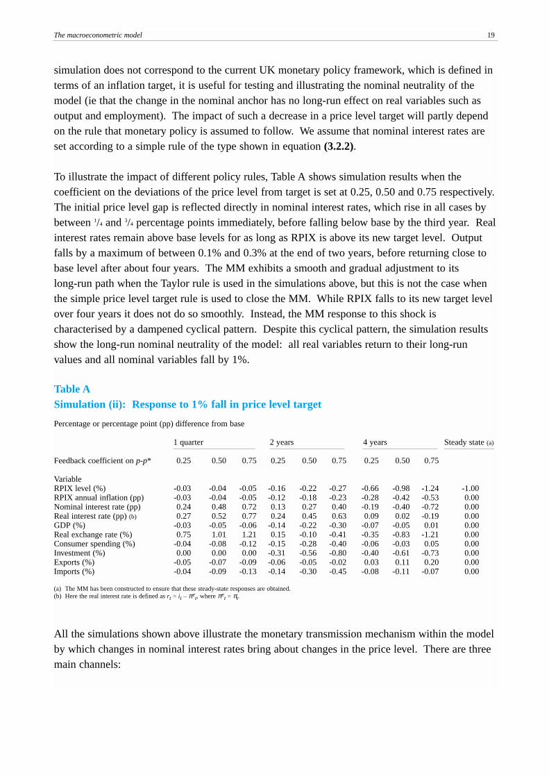
To illustrate the impact of different policy rules, Table A shows simulation results when thecoefficient on the deviations of the price level from target is set at 0.25, 0.50 and 0.75 respectively.The initial price level gap is reflected directly in nominal interest rates, which rise in all cases bybetween 1/4 and 3/4 percentage points immediately, before falling below base by the third year. Realinterest rates remain above base levels for as long as RPIX is above its new target level. Outputfalls by a maximum of between 0.1% and 0.3% at the end of two years, before returning close tobase level after about four years. The MM exhibits a smooth and gradual adjustment to its long-run path when the Taylor rule is used in the simulations above, but this is not the case whenthe simple price level target rule is used to close the MM. While RPIX falls to its new target levelover four years it does not do so smoothly. Instead, the MM response to this shock ischaracterised by a dampened cyclical pattern. Despite this cyclical pattern, the simulation resultsshow the long-run nominal neutrality of the model: all real variables return to their long-runvalues and all nominal variables fall by 1%.

All the simulations shown above illustrate the monetary transmission mechanism within the modelby which changes in nominal interest rates bring about changes in the price level. There are threemain channels:

Table ASimulation (ii): Response to 1% fall in price level target

Percentage or percentage point (pp) difference from base

1 quarter 2 years 4 years Steady state (a)

Feedback coefficient on p-p* 0.25 0.50 0.75 0.25 0.50 0.75 0.25 0.50 0.75

VariableRPIX level (%) -0.03 -0.04 -0.05 -0.16 -0.22 -0.27 -0.66 -0.98 -1.24 -1.00RPIX annual inflation (pp) -0.03 -0.04 -0.05 -0.12 -0.18 -0.23 -0.28 -0.42 -0.53 0.00Nominal interest rate (pp) 0.24 0.48 0.72 0.13 0.27 0.40 -0.19 -0.40 -0.72 0.00Real interest rate (pp) (b) 0.27 0.52 0.77 0.24 0.45 0.63 0.09 0.02 -0.19 0.00GDP (%) -0.03 -0.05 -0.06 -0.14 -0.22 -0.30 -0.07 -0.05 0.01 0.00Real exchange rate (%) 0.75 1.01 1.21 0.15 -0.10 -0.41 -0.35 -0.83 -1.21 0.00Consumer spending (%) -0.04 -0.08 -0.12 -0.15 -0.28 -0.40 -0.06 -0.03 0.05 0.00Investment (%) 0.00 0.00 0.00 -0.31 -0.56 -0.80 -0.40 -0.61 -0.73 0.00Exports (%) -0.05 -0.07 -0.09 -0.06 -0.05 -0.02 0.03 0.11 0.20 0.00Imports (%) -0.04 -0.09 -0.13 -0.14 -0.30 -0.45 -0.08 -0.11 -0.07 0.00

(a) The MM has been constructed to ensure that these steady-state responses are obtained.(b) Here the real interest rate is defined as rt = it – πe

t, where πet = πt.


● First, the real exchange rate appreciates on impact by around 1%, before depreciating backtowards its base value.(1) This initial jump reflects the anticipated cumulative policy-induced rise in the real interest rate over the entire simulation. The short-termappreciation has a direct effect on domestic prices, partly through the influence of importprices on retail prices and partly through the temporary effect of the real exchange rate onreal wages. There is also an indirect effect on prices via net trade. Exports initially fall byaround 0.1% before recovering as the real exchange rate falls back. Imports are stimulatedby the fall in competitiveness, but this is outweighed by the effects of the fall in domesticdemand. The net impact is for imports to fall by 0.3% after two years.

● Second, higher nominal interest rates result in the stock of net financial wealth beingdevalued. That, together with the short-term confidence effects, results in lowerconsumption in the short run. Consumption falls by about 0.3% after two years. Furtherout, this is offset by a terms-of-trade effect on income and by a wealth effect associated withthe exchange rate appreciation.

● Third, there is the effect of real interest rates on investment and consumption, withinvestment falling by about 0.6% at the end of two years. In the longer run, investmentrecovers to bring the capital stock back towards its long-run level, but this occurs slowlybecause of the protracted response of investment in the model. Similarly, as real interestrates and wealth return to their long-run level, consumption also returns to its long-run level.

6 Detailed equation listing

This section describes, in detail, the equations that form the Bank’s macroeconometric model(MM). It is important to note that the equations outlined in this section have been developed aspart of the overall structure of the MM. The structure of the equations, the short-run and long-runrestrictions placed on the coefficients, the available set of variables and the choice of data have allbeen dictated by the structure of the MM. The criteria for selection of a particular equationinclude the equation’s statistical properties and its impact on the overall MM simulation properties.For these reasons the individual equations outlined in this section should not be viewed as the‘best’ single equations estimated: they are part of a system of equations that form the MM. Fromtime to time alternative equations are developed and examined as part of the MM structure. Theymay be used to examine the impact of alternative economic theories, or the impact of relaxingsome of the restrictions placed on the equations.

Several conventions are used in the presentation of the equations in this section. Lower-caseletters indicate natural logs. The subscript t denotes time: data are quarterly. ∆ indicates a firstdifference. Q1, Q2, Q3 and Q4 denote seasonal dummies. Each relationship is written so as todistinguish the long-run solution of the equation from the short-run dynamics. Long-run solutions

(1) This description of the transmission mechanism applies to all the simulations shown, but the quantitative results apply to the price leveltarget shock with a monetary policy rule of the form (3.2.2), with the feedback parameter set to 0.5. Altering assumptions under which thesimulations are performed may alter the transmission mechanism as described here. For example, the transmission mechanism might differif inflation expectations were assumed to evolve differently or if real interest rates were assumed to be affected by temporary monetarypolicy shocks.


appear in square brackets, and follow from the usual practice of estimating error-correctionmodels. T-values are shown in parentheses, where applicable. Single-equation dynamic responsesare given for some key variables. A standard set of diagnostic tests is shown, with the probabilityvalues for the diagnostic tests given in square brackets. Definitions and data sources for all modelvariables are given at the end of the equation listing. Bold numbers in brackets are cross-references to equations.

6.1 Money, financial and wealth variables

6.1.1 Three-month interest rate (RS)

The usual settings are either an exogenous constant nominal rate or market interest rate path (thealternative conditioning assumptions in Inflation Report projections), or a simple form of theTaylor rule linking the short-term nominal interest rate to the monetary policy target variable.

(6.1.1)

where

RS = base rate of interest (6.1.1).INF = four-quarter inflation rate of RPIX.GDPT = trend output (6.2.5).GDP = GDP(A) at factor cost (6.2.1).ZPSTA = Government inflation target (exogenous).

Θ0, Θ1 and Θ2 are parameters to be set by the user.

A variant of the rule links short nominal rates to a price level target.

(6.1.1a)

where

RS = base rate of interest (6.1.1).INF = four-quarter inflation rate of RPIX.GDPT = trend output (6.2.5).GDP = GDP(A) at factor cost (6.2.1).RPIX = RPI excluding mortgage interest payments (6.4.6).RPIX* = target level for RPIX (exogenous).

6.1.2 Twenty-year bond rates (RL)

For simulation purposes, long rates are set by reference to current short rates.

RLt = RSt (6.1.2)

where

RS INF gdp gdpt rpix rpixt t t t t t= + + −( ) + −( )Θ Θ Θ0 1 2*

RS INF gdp gdpt INF ZPSTAt t t t t t= + + −( ) + −( )Θ Θ Θ0 1 2


RL = 20-year bond yield (6.1.2).RS = base rate of interest (6.1.1).

6.1.3 Mortgage interest rates (RMM4)

Mortgage interest rates affect the mortgage interest payment sub-index of the RPI. They areproxied by a constant mark-up over a weighted average of current and lagged short-term interestrates. Lagged rates are used to reflect some of the delay between official rate changes and theirpass-through to mortgage borrowers. Both the weights and the mark-up were chosen toapproximate past experience.

(6.1.3)

where

RMM4 = mortgage interest rate (6.1.3).RS = base rate of interest (6.1.1).

6.1.4 Deposit interest rates (RD)

Combined with the short-term interest rate, the deposit rate defines the opportunity cost of holdingmoney. In the long run, it is equal to a proportion of the short-term rate (6.1.1).

(6.1.4)

where

RD = deposit rate (6.1.4).RS = base rate of interest (6.1.1).

Adjusted R2 = 0.80Equation standard error = 0.38LM test for serial correlation: F-stat. = 1.79 [0.17] Normality test: χ2(2) = 57.12 [0.00]Heteroscedasticity: F-stat. = 1.12 [0.36] Sample period: 1977 Q3–1998 Q2

6.1.5 Real cost of capital (RCC)

Investment is affected by the real cost of capital (RCC). This reflects the rate of depreciation (on aquarterly basis), and the rates of both corporate taxation and investment allowances. As elsewherein the model, inflation expectations relate to RPIX.

(6.1.5)

where

RCCPVIC

RCRL INFE BETAt

t

tt t t= −

−

− + −( )( )0 002511

100 1 4.

∆ ∆ ∆ ∆RD RD RS RS RD RSt t t t t t

(1.4) ( 2.7) (17.4) (3.0) ( 2.8)

= − + + − −− − − −− −

0 0572 0 28 0 75 0 24 0 13 0 71 1 1 1. . . . . [ . ]

RMM4 RS RSt t t= ( ) + ( ) +−23

13 1 1 0.


RCC = real cost of capital (6.1.5).PVIC = present value of investment allowances (exogenous).RC = effective corporate income taxation rate (exogenous).RL = 20-year bond yield (6.1.2).INFE = expectations of annual RPIX inflation (6.4.16).1–BETA = business sector net capital stock depreciation rate (exogenous).

6.1.6 Nominal effective exchange rate (EER)

For simulation purposes, the exchange rate is modelled using uncovered interest parity (UIP), withmodel-consistent expectations.

eert = xeert + RSDF (6.1.6)

where

EER = sterling effective exchange rate index (6.1.6).XEER = expected sterling effective exchange rate (one period ahead).RSDF = interest rate differential (6.1.7).

The interest rate differential is defined by:

(6.1.7)

where

RS = base rate of interest (6.1.1).WRS = world nominal interest rate (exogenous).

But under certain forecasting conditions the exchange rate is assumed to evolve along a pathhalfway between a constant rate and the path implied by the UIP condition, with backward-lookingexpectations and conditional on constant interest rates.

For simulation purposes, the sterling-dollar exchange rate (EDS) is simply related to the effectiverate. The constant reflects different units of measurement.

edst = – 4.02 + eert (6.1.8)

EDS = sterling-US dollar exchange rate (6.1.8).EER = sterling effective exchange rate index (6.1.6).

6.1.7 Real exchange rate (RXRX, RXRM and RRX)

The exporters’ real exchange rate (RXRX) is the effective exchange rate deflated using relativeexport prices. The importers’ relative price (RXRM) is the price of imports relative to the GDPdeflator. A further measure (RRX) relates the GDP deflator to world export prices.

RSDFRS WRSt t= +

− +

log log1

4001

400


(6.1.9)

where

RXRX = exporters’ real exchange rate (6.1.9).EER = sterling effective exchange rate index (6.1.6).WPX = world export prices (exogenous).PX = export price deflator (6.4.3).

(6.1.10)where

RXRM = importers’ relative price (6.1.10).PM = import price deflator (6.4.2).PGDP = GDP deflator at factor cost (6.4.1).

(6.1.11a)

where

RRX = real exchange rate (GDP deflator measure) (6.1.11).EER = sterling effective exchange rate index (6.1.6).WPX = world export prices (exogenous).PGDP = GDP deflator at factor cost (6.4.1).

To solve the model in forward-looking mode, it is convenient to express the UIP condition in realterms.

(6.1.11b)

where

RRX = real exchange rate (GDP deflator measure) (6.1.11).XRRX = expected real exchange rate (one period ahead).RSDF = interest rate differential (6.1.7).XWPX = expected M6 export prices (one period ahead) (exogenous).PGDP = GDP deflator at factor cost (6.4.1).WPX = world export prices (exogenous).XPGDP = expected GDP deflator at factor cost (one period ahead).

When the real exchange rate is determined in this way, the nominal exchange rate is obtained byinverting the identity for RRX in (6.1.11a).

rrx xrrx RSDF xwpx pgdp wpx xpgdpt t t t t t t= + + + − −

RRXEER PGDP

WPXtt t

t= .

RXRMPM

PGDPtt

t=

RXRXEER PX

WPXtt t

t= .


6.1.8 Household sector wealth (WEL)

Household sector wealth (WEL) is modelled in two parts: gross housing wealth and net financialwealth (GHW and NFW).

WELt = GHWt + NFWt (6.1.12)

Nominal housing investment is the flow into nominal housing wealth. The stock of nominalhousing wealth is revalued in line with changes in house prices.

(6.1.13)

where

GHW = gross housing wealth (6.1.13).PGDP = GDP deflator at factor cost (6.4.1).IH = private sector dwellings investment (6.2.13).PHSE = UK house prices (6.4.15).

Saving is the flow into nominal net financial wealth. The stock of net financial wealth is revaluedin line with changes in asset prices (REV).

(6.1.14)

where

NFW = net financial wealth (6.1.14).PC = total final consumers’ expenditure deflator (6.4.13).RHPI = real household post-tax income (6.6.5).C = consumers’ expenditure (6.2.8).IH = private sector dwellings investment (6.2.13).REV = wealth revaluation term (6.1.15).

The weights in the revaluation term were derived from the household sector balance sheet (inFinancial Statistics) and reflect the relative importance of foreign assets, gilts, interest-bearingdeposits and equities in net financial wealth.

(6.1.15)

where

REV = wealth revaluation term (6.1.15).EER = sterling effective exchange rate index (6.1.6).

REVEER

EER

WEQP

WEQP

EER

EER

RL

RL

EER

EER

USRL

USRL

EQP

EQP

tt

t

t

t

t

t

t

t

t

t

t

t

t

t

= +

+

+

+

+

−

−

− −

− −

−

0 045 0 12 0 01 0 15

0 04 0 64

1

1

1 1

1 1

1

. . . .

. .

NFW PC RHPI C IH NFW REVt t t t t t t= − −( ) + −1.

GHW PGDP IH GHWPHSE

PHSEt t t tt

t= ( ) +

−

−. 1

1


WEQP = world equity prices (exogenous).RL = 20-year bond yield (6.1.2).USRL = US long bond rate (exogenous).EQP = equity prices (6.1.16).

An alternative, used in forecasting, is to allow NFW to evolve in line with nominal GDP.

Equity prices either evolve in line with a simple dividend growth model.

(6.1.16a)

where

EQP = equity prices (6.1.16).GDPL = GDP at factor cost in current prices (6.2.4).RL = 20-year bond yield (6.1.2).

Or in line with nominal GDP, supplemented by an exogenous constant (risk premium).

∆eqpt = ∆gdplt + 0.02 (6.1.16b)

where

EQP = equity prices (6.1.16).GDPL = GDP at factor cost in current prices (6.2.4).RL = 20-year bond yield (6.1.2).

The simpler nominal GDP growth equation (6.1.16b) was adopted for the simulations.

6.1.9 Broad money demand (M4)

Real broad money holdings respond to activity, net financial wealth and interest rates. Money canbe specified as the nominal anchor in a monetary policy rule for interest rates.

(6.1.17)

∆ ∆ ∆ ∆m pgdp m pgdp gdpm gdpm

m pgdp gdpm

nfw pgdp gdpm

RD RS

t t t t

(4.2) (3.3) (3.1) ( 1.8)

t t t

( 1.9)

t t t

( 77.6)

t t

( 4.8)

4 0 0077 0 33 4 0 45 0 28

0 037 4

0 60

0 022

1 1

1 1 1

1 1 1

1 1

−( ) = + −( ) + −

− − −

− − −( )

− −( )

− −

−

− − −−

− − −

−

− −

−

. . . .

. [

.

. ]

EQPgdpl

RL gdplGDPLt

t

t tt= +

−

0 00071

100.

( )( / )

( )∆

∆


where

M4 = broad money (6.1.17).GDPM = GDP(A) at constant market prices (6.2.3).PGDP = GDP deflator at factor cost (6.4.1).NFW = net financial wealth (6.1.14).RD = deposit rate (6.1.4).RS = base rate of interest (6.1.1).

Adjusted R2: 0.28Equation standard error: 0.011LM test for serial correlation: F-stat. = 2.12 [0.13]Normality test: χ2(2) = 1.73 [0.42]Heteroscedasticity: F-stat. = 1.60 [0.14]Sample period: 1977 Q3–2000 Q1

6.2 Demand and output

6.2.1 Gross domestic product (GDP, GDPM, GDPL)

Expenditure-based GDP is an accounting identity, including domestic demand, imports, exportsand the factor cost adjustment.

GDPt = DDt + Xt – Mt – FCAt (6.2.1)

where

GDP = GDP(A) at factor cost (6.2.1).DD = total domestic expenditure (6.2.7).X = exports of goods and services (6.2.18).M = imports of goods and services (6.2.19).FCA = factor cost adjustment (6.2.2).

The factor cost adjustment is an (estimated) function of GDP.

fcat = –1.87 + gdpt (6.2.2)

where

FCA = factor cost adjustment (6.2.2).GDP = GDP(A) at factor cost (6.2.1).

GDPM is expenditure-based GDP at constant 1995 market prices.

GDPMt = GDPt + FCAt (6.2.3)


where

GDPM = GDP(A) at constant market prices (6.2.3).GDP = GDP(A) at factor cost (6.2.1).FCA = factor cost adjustment (6.2.2).

Nominal GDP (GDPL) at factor cost is the product of GDP (6.2.1) and the GDP deflator (PGDP)(6.4.1).

GDPLt = PGDPt .GDPt (6.2.4)

6.2.2 Trend GDP and capacity utilisation (GDPT, CAPU)

Trend output is determined by an estimated Cobb-Douglas production function. The direct inputsare the non-residential capital stock, the level of population of working age and exogenous labour-augmenting technical progress captured by the time trend.

(6.2.5)

where

GDPT = trend output (6.2.5).KNH = capital stock excluding residential housing (6.2.10).POWA = population of working age (exogenous).TIME = time trend.


Capacity utilisation is proxied by the residuals from the estimation of a production function wherethe direct inputs are employment measured in hours, the non-residential capital stock and labour-augmenting technical progress captured by the time trend.

(6.2.6)

where

CAPU = capacity utilisation (6.2.6).GDP = GDP(A) at factor cost (6.2.1).EMPH = total employment in hours (6.3.11).

CAPU gdp emph knh TIMEt t t t

(288.0) ( 34.1)

= − − − −−

2 66 0 70 0 30 0 70 0 004. . . ( . )( . )

gdpt knh powa TIMEt t t

(3.9) (18.7)

= + + +0 063 0 3 0 7 0 70 0 004. . . ( . )( . )


KNH = capital stock, excluding residential housing (6.2.10).TIME = time trend.


6.2.3 Domestic demand (DD)

Domestic demand is determined by an accounting identity, as the sum of consumers’ expenditure,investment, government consumption and stockbuilding.

DDt = Ct + It + Gt + IIt (6.2.7)

where

DD = total domestic expenditure (6.2.7).C = consumers’ expenditure (6.2.8).I = fixed investment (6.2.9).G = general government final consumption expenditure (exogenous), (see Section 6.2.10).II = net stockbuilding (6.2.16).

6.2.4 Consumers’ expenditure (C)

In the long run, consumers’ expenditure is a function of wealth, labour income and real interestrates. Nominal rates are included in the short run of the equation to capture confidence and cash-flow effects of changes in the stance of monetary policy. Changes in the unemployment rateare also included, to capture precautionary saving influences.

(6.2.8)

where

C = consumers’ expenditure (6.2.8).LY = real post-tax labour income (6.6.6).YDIJ = non-labour income (6.6.4).PC = total final consumers’ expenditure deflator (6.4.13).

∆ ∆ ∆ ∆ ∆

∆ ∆ ∆

c ly ydij pc ur ghw pc

nfw pc RS RS

c ly

t t t t t t t

( 2.7) (3.6) (4.0) ( 3.5) (4.8)

t t t t

(1.3) ( 2.4) ( 2.8)

t t

= − + + −( ) − + −

+ − − −

− − −

− − −

− −

−− −

− −

0 036 0 19 0 052 0 068 0 14

0 014 0 0016 0 0017

0 17 0 89 0

1 1 1

1

1 1

. . . . . ( )

. ( ) . .

. . .. ( ) . ( )11 0 00281 1 2 2wel pc RS INFEt t t t

( 4.3) (3.6) (2.3)

− − − −

−

− + −[ ]


UR = rate of unemployment (6.3.8).GHW = gross housing wealth (6.1.13).NFW = net financial wealth (6.1.14).WEL = total household sector wealth (6.1.12).RS = base rate of interest (6.1.1).INFE = expectations of annual RPIX inflation (6.4.16).


Single-equation dynamic responses:

Response of consumers’ expenditure level to a 1% shock to RHS variablesPer cent

Quarters ahead Real labour Real net Real gross Real interest rateincome financial wealth housing wealth

1 0.3 0.02 0.12 0.0004 0.6 0.04 0.09 -0.0018 0.7 0.06 0.07 -0.002Long run (LR) 0.9 0.07 0.05 -0.00350% of LR by 3 quarters 3 quarters o/s 6 quarters90% of LR by 11 quarters 12 quarters o/s 15 quarters

Per centQuarters ahead Nominal Unemployment Real non-labour

interest rate rate income1 -0.003 -0.07 0.054 -0.002 -0.04 0.038 -0.0 -0.02 0.01Long run (LR) 0.0 0.0 0.0

o/s = overshoots eventual long-run response in short term.

6.2.5 Fixed investment (I)

Fixed investment is the sum of business investment, housing investment and governmentinvestment.

It = IBUSt + IHt + IGt (6.2.9)

where


I = fixed investment (6.2.9).IBUS = business investment (6.2.12).IH = private sector dwellings investment (6.2.13).IG = general government investment (exogenous), (see Section 6.2.9).

6.2.6 The capital stock (KNH, KBUSNH)

The capital stock is the previous period’s stock (allowing for depreciation at the exogenous rate(1–BETA)) plus current investment. 21% of government investment is assumed to be housing,consistent with the average historical relationship.

KNHt = BETANH.KNHt–1 + It – IHt – 0.21IGt (6.2.10)

KBUSNHt = BETA.KBUSNHt–1 + IBUSt (6.2.11)

where

KNH = capital stock, excluding residential housing (6.2.10).KBUSNH = business non-residential capital stock (6.2.11).1–BETANH = whole-economy net capital stock net of housing depreciation rate (exogenous).1–BETA = business sector net capital stock depreciation rate (exogenous).IG = general government investment (exogenous), (see Section 6.2.9).IBUS = business investment (6.2.12).

6.2.7 Business investment (IBUS)

The assumed Cobb-Douglas production technology implies that the capital-output ratio is afunction of the user cost of capital with a unit coefficient in the long run. But adjustment issluggish.

(6.2.12)

where

IBUS = business investment (6.2.12).GDP = GDP(A) at factor cost (6.2.1).KBUSNH = business non-residential capital stock (6.2.11).RCC = real cost of capital (6.1.5).DUMMY = 1985 Q2.

∆ ∆ ∆ ∆

∆ ∆

ibus ibus ibus ibus

ibus gdp

ibus kbusnh kbusnh gdp rcc

dummy

t t t t

( 1.9) (1.0) (1.7) (1.8)

t t

(1.7) (1.5)

t t t t t

( 1.9)

= − + + +

+ +

− + − + − +

+

− − −−

− −

− − − − −−

0 054 0 11 0 19 0 18

0 17 1 0

0 047 3 09 0 27

1 2 3

4 1

1 2 2 2 1

. . . .

. .

. [ . . ( )]


Adjusted R2: 0.36Equation standard error: 0.028 LM test for serial correlation: F-stat. = 1.35 [0.27]Normality test: χ2(2) = 2.28 [0.32]Heteroscedasticity: F-stat. = 1.60 [0.10]Sample period: 1983 Q2–1999 Q3


Response of business investment level to a 1% shock to RHS variablesPer cent

Quarters ahead Real cost GDP outputof capital

1 -0.01 1.04 -0.06 1.48 -0.01 1.6Long run (LR) -0.27 0.27

The structure of the entire supply side of the MM (including capital accumulation (6.2.11) and theproduction function (6.3.11)) ensures that in the long run a 1% increase in the real cost of capitalwill result in a 1% decrease in the level of business investment and the capital-output ratio.

6.2.8 Private sector dwellings investment (IH)

Private sector dwellings investment (IH) follows the growth of business investment.

∆iht = ∆ibust (6.2.13)

where

IH = private sector dwellings investment (6.2.13).IBUS = business investment (6.2.12).

6.2.9 Government investment (IG)

In the simulations described in Section 5, real government investment (IG) is assumed to beexogenous. Nominal government investment (IGL) is derived by identity using the overall GDPdeflator (6.4.1). But announced nominal government spending plans provide the basis forforecasting this component, with real spending defined by the inverse of equation (6.2.14) below.

IGLt = IGt . PGDPt (6.2.14)

6.2.10 Government consumption (GL)

In the simulation described in Section 5, real government consumption (G) is assumed to beexogenous. Nominal government consumption (GL) is derived by identity using the government


consumption deflator (PG) (6.4.14). But announced nominal government spending plans providethe basis for forecasting this component, with real spending then defined by the inverse ofequation (6.2.15) below.

GLt = Gt . PGt (6.2.15)

6.2.11 Stockbuilding (II)

Net stockbuilding is defined as the change in total stocks.

IIt = KIIt – KIIt–1 (6.2.16)

where

II = net stockbuilding (6.2.16).KII = stock level (6.2.17).

In the medium term, the stock-output ratio follows a downward (time) trend.

(6.2.17)

where

KII = stock level (6.2.17).GDP = GDP(A) at factor cost (6.2.1).TIME = time trend.


6.2.12 Export volumes of goods and services (X)

Both of the trade volume equations are modelled as a function of relative prices and total demandfor exports or imports (proxied by world trade (TRAD) (exogenous) and domestic demand (DD)(6.2.7) respectively).

(6.2.18)

∆ ∆ ∆ ∆x x rxrx trad

x trad rxrx dummy

t t t t

(2.9) ( 2.8) ( 1.3) (1.5)

t t t

( 2.9) (1.7)

= − − +

− − +[ ] +

−− −

− − −

−

0 72 0 33 0 10 0 30

0 11 0 69

1

1 1 1

. . . .

. .

∆ ∆ ∆kii gdp gdp kii gdp TIMEt t t t t t

(1.9) (1.2) (1.8) ( 2.5)

= + + − − +[ ]− − − − −

−

0 03 0 14 0 26 0 13 0 0041 2 1 1 1. . . . .


where

X = exports of goods and services (6.2.18).RXRX = exporters’ real exchange rate (6.1.9).TRAD = world trade (exogenous).DUMMY = 1991 Q1.



Response of export volume level to a 1% shock to RHS variablesPer cent

Quarters ahead Exporters’ real World tradeexchange rate

1 -0.1 0.34 -0.3 0.58 -0.5 0.6Long run (LR) -0.7 1.050% of LR by 7 quarters 5 quarters90% of LR by 26 quarters 24 quarters

6.2.13 Import volumes of goods and services (M)

(6.2.19)

where

M = imports of goods and services (6.2.19).DD = total domestic expenditure (6.2.7).RXRM = importers’ relative price (6.1.10).SPEC = trade specialisation term (exogenous).DUMMY = 1981 Q1.

Adjusted R2: 0.64Equation standard error: 0.018 LM test for serial correlation: F-stat. = 0.12 [0.95]Normality test: χ2(2) = 106.1 [0.0]

∆ ∆m dd m dd rxrm SPEC

dummy

t t t t t t

( 3.3) (8.3) ( 3.3) (1.1) ( 5.6)

= − + − − + −[ ]

+

− − − −

− − −

0 25 1 73 0 21 0 22 0 901 1 1 1. . . . .


Heteroscedasticity: F-stat. = 1.12 [0.36]Sample period: 1980 Q2–1997 Q4


Response of import volume level to a 1% shock to RHS variablesPer cent

Quarters ahead Importers’ relative Domestic demand Specialisationprice

1 0.0 1.7 0.04 -0.1 1.3 0.58 -0.1 1.1 0.8Long run (LR) -0.2 1.0 0.950% of LR by 3 quarters o/s 3 quarters90% of LR by 10 quarters o/s 10 quarters


6.2.14 Balance of payments (BAL, BALT, BIPD and BTRF)

The current account balance (BAL) is determined by an accounting identity. It is the sum of thenominal trade balance (BALT), the balance of interest, dividends and profits (BIPD) and thebalance of transfers (BTRF) (exogenous).

BALt = BALTt + BIPDt + BTRFt (6.2.20)

The nominal balance of trade is also defined by an accounting identity.

BALt = Xt . PXt – Mt . PMt (6.2.21)

where

BALT = nominal balance of trade (6.2.21). X = exports of goods and services (6.2.18).M = imports of goods and services (6.2.19).PX = export price deflator (6.4.3).PM = import price deflator (6.4.2).

The balance of interest payments, dividends and profits (BIPD) is proxied by the product of theexogenous world nominal interest rate (WRS) and the average net external assets (NEA) over thecurrent and past quarter.

(6.2.22)

where

BIPDNEA NEA

tt t t=

+

−WRS

400 21


BPID = balance of interest, dividends and profits (6.2.22).WRS = world nominal interest rates (exogenous).NEA = net external assets (6.2.23).

6.2.15 Net external assets (NEA)

Net external assets are defined as the difference between gross UK holdings of foreign assets(UKA) (6.2.24) and foreign holdings of UK assets (FOH) (6.2.25).

NEAt = UKAt – FOHt (6.2.23)

Both gross UK and foreign asset holdings are modelled using a simple stock/flow framework. Thecurrent account balance (assumed equal to the capital account balance) gives the flow apportionedto the two stocks according to their average ratio across the 1990s.

(6.2.24)

where

UKA = UK holdings of foreign assets (6.2.24).BAL = current account balance (6.2.20).WPX = world export prices (exogenous).EER = sterling effective exchange rate index (6.1.6).

(6.2.25)

where

FOH = foreign holdings of UK assets (6.2.25).BAL = current account balance (6.2.20).PGDP = GDP deflator at factor cost (6.4.1).

6.3 Labour market

6.3.1 Average earnings (EARN)

The labour market earnings equation is based on a forward-looking model of contract dynamics.

The desired or target wage (W*) is defined as:

wt* = pgdpt + gdpt – empt – remt – 0.013 URt + ZPROXY (6.3.1)

where

PGDP = GDP deflator at factor cost (6.4.1).UR = rate of unemployment (6.3.8).

FOH BAL FOHPGDP

PGDPt t tt

t= − +

−

−0 49 1

1.

UKA BAL UKAWPX WPX

EER EERt t tt t

t t= +

−

−

−0 51 1

1

1.


ZPROXY = measure of structural effects of labour market developments (exogenous).GDP = GDP(A) at factor cost (6.2.1).EMP = level of employment in heads (6.3.12).REM = effective employers’ social contribution tax rate (exogenous).

ZPROXY is designed to capture movements in unobservable structural variables that affect thelabour market (such as union power and the replacement ratio), and is derived by fitting a Hodrick-Prescott filter through data on the labour share of income and the unemployment rate.

Following Moghadam and Wren-Lewis (1994), the pure theoretical model of contract dynamicssets earnings each period equal to a backward and a forward convolution of expected wages,wstarc, where:

(6.3.2)

and w*i,j is the expectation of w*

j formed at time i.

In estimation, these forward-looking terms are treated as rational. The estimated equation alsoembodies the assumption that wage-setters partly adopt a rule of thumb in setting their contracts(using a combination of lagged wage growth and current growth of retail prices and productivity todetermine their wage settlements) in addition to explicitly forward-looking considerations.

(6.3.3)

where

EARN = average earnings index (6.3.3).RP = RPIX plus productivity (6.3.4).


earn earn earn earn earn

earn earn earn earn

rp rp rp rp

t t t t t

(26.7) (6.0)

t t t t

(10.1)

t t t t

= + + +

+ + + +

+ − + + ++ −

− − − −

− − − −

− − −

0 79 0 63 0 25

2 5 0 65

2 5 1 0 65

1 0 63

1 2 3 4

1 2 3 4

1 2 3

. { . ( . )[( )

( . ) . ( )

( . ) ( . )( )]

( .

∆ ∆ ∆ ∆

∆ ∆ ∆ ∆)[)[ . ( . ) ]} ( . )earn earn rp wstarct t t t− −+ + − + −1 10 65 1 0 65 1 0 79∆ ∆

wstarc w w w w

w w w w

w w w w

w

t t t t t t t t t

t t t t t t t t

t t t t t t t t

t

= + + +

+ + + +

+ + + +

+

∗ ∗+

∗+

∗+

∗− −

∗−

∗− +

∗− +

∗− −

∗− −

∗−

∗− +

∗

( / )( , , , ,

, , , ,

, , , ,

1 16 1 2 3

1 1 1 1 1 1 2

2 2 2 1 2 2 1

−− −∗

− −∗

− −∗

−+ + +3 3 3 2 3 1 3, , , , ),t t t t t t tw w w


rpt = rpixt + gdpt – empt (6.3.4)

where

RP = RPIX inflation adjusted by productivity (6.3.4).RPIX = RPI excluding mortgage interest payments (6.4.6).GDP = GDP(A) at factor cost (6.2.1).EMP = level of employment in heads (6.3.12).

In simulations, expected future values of w* (where w*ij is the expectation of w*j formed at time i)can be treated in different ways. Either as a model-consistent expectation.

w*t,t+1 = w*

t+1 ; w*t,t+2 = w*

t+2 ; w*t,t+3 = w*

t+3 (6.3.5)

Or as the result of a backward-looking rule, as adopted in the simulations.

(6.3.6)

for m = 1, 2 and 3.


Response of the level of earnings to a 1% shock to RHS variablesPer cent

Quarters ahead GDP deflator Productivity Unemployment1 0.2 0.5 -0.24 0.6 1.1 -0.78 0.9 1.2 -1.2Long run (LR) 1.0 1.0 -1.350% of LR by 4 quarters o/s 4 quarters90% of LR by 8 quarters o/s 8 quarters


6.3.2 Unemployment level, unemployment rate, participation rate (UN, UR, PA)

The level of unemployment (UN) is modelled as an identity, relating unemployment to changes inemployment (EMP), the population aged 16 and over (POP) (exogenous) and the participation rate (PA).

UNt = PAt . POPt – EMPt (6.3.7)

w pgdp gdp emp rem UR ZPROXY

m INFE

m GDP EMP GDP EMP

GDP EMP

t t m t t t t t t

t

t t t t

t t

∗+

− −

− −

= + − − − +

+ +

+ + ( ) − ( )( )

, .

log.

log/ /

/

0 013

1400

1 44 4

4 4


where

UN = level of unemployment (6.3.7).PA = participation rate (6.3.9).POP = population aged 16 and over (exogenous).EMP = level of employment in heads (6.3.12).

The rate of unemployment (UR) is an identity.

(6.3.8)

where

UR = rate of unemployment (6.3.8).UN = level of unemployment (6.3.7).EMP = level of employment in heads (6.3.12).

and the participation rate is given by:

(6.3.9)

where

PA = participation rate (6.3.9).INWA = proportion of population of working age that is inactive (6.3.10).POWA = population of working age (exogenous).POP = population aged 16 and over (exogenous).INOLD = proportion of population over retirement age that is inactive (exogenous).

INWA can be assumed invariant to the economy cycle or modelled by a simple cyclical influencederived from lagged employment (as a proportion of the working-age population). The latterassumption was used in the simulations described in Section 5.

(6.3.10)

where

INWA = proportion of population of working age that is inactive (6.3.10).EMP = level of employment in heads (6.3.12).POWA = population of working age (exogenous).TIME = time trend.

INWAEMP

POWA

EMP

POWATIME INWAt

t

t

t

tt

(2.3) ( 5.6) (4.2) (2.9) (16.6)

= −

+

+ +−

−

−

−−

−

0 06 0 25 0 20 0 00006 0 871

1

2

21. . . . .

PA INWAPOWA

POPINOLD

POWA

POP= −

− −

1 1

URUN

EMP UNtt

t t=

+

100


Adjusted R2: 0.98Equation standard error: 0.001 Sample period: 1984 Q1–1998 Q4

6.3.3 Employment in hours (EMPH)

Long-run employment in hours is derived from an inverted production function. Changes in GDPappear in the dynamic hours equation.

(6.3.11)

where

EMPH = total employment in hours (6.3.11).GDP = GDP(A) at factor cost (6.2.1).CAPU = capacity utilisation (6.2.6).


Single-equation dynamic responses for equation:

Response of employment in hours level to a 1% shock to RHS variablesPer cent

Quarters ahead GDP output Capital stock1 0.3 0.04 0.9 -0.28 1.3 -0.4Long run (LR) 1.4 -0.450% of LR by 3 quarters 5 quarters90% of LR by 7 quarters 10 quarters

6.3.4 Employment in heads (EMP)

Employment in heads (EMP) can be written as:

(6.3.12)

where

EMP = level of employment in heads (6.3.12).EMPH = total employment in hours (6.3.11).

EMPEMPH

AVHtt

t=

∆ ∆ ∆emph emph gdp CAPUt t t t

( 1.3) (4.9) (4.3) (4.6)

= − + + + [ ]− −

−

0 0008 0 43 0 28 0 171 1. . . .


AVH = average hours per worker (6.3.13).

6.3.5 Average hours per worker (AVH)

Average hours per worker is a decreasing function of the extent of part-time working, and iscyclical about a long-run trend.

(6.3.13)

where

AVH = average hours per worker (6.3.13).PTSH = part-time share of employment (exogenous).CAPU = capacity utilisation (6.2.6).


Single-equation dynamic responses for equation:

Response of average hours level to a 1% shock to RHS variablesPer cent

Quarters ahead Part time share Capacity utilisation1 -0.6 0.04 -0.6 0.38 -0.6 0.7Long run (LR) -0.6 1.450% of LR by 1 quarter 9 quarters90% of LR by 1 quarter 25 quarters

6.3.6 Unit labour costs (ULC)

Nominal unit labour costs (ULC) are defined by the following identity:

(6.3.14)

where

ULC = nominal unit labour costs (6.3.14).

ULCEARN REM EMP

GDPtt t t

t= . .

∆ ∆

∆ ∆

avh avh avh

PTSH PTSH PTSH CAPU

t t t

( 2.4) ( 2.4) (3.0)

t t t t

(3.2)

= − − +

− − + +

− −− −

− − −

0 21 0 06 0 32

0 61 0 32 0 06 0 09

1 1

1 1 1

. . .

. ( . . ) .


EARN = average earnings index (6.3.3). REM = effective employers’ social contribution tax rate (exogenous).EMP = level of employment in heads (6.3.12).GDP = GDP(A) at factor cost (6.2.1).

6.4 Prices

6.4.1 Domestic output prices—the GDP deflator (PGDP)

The PGDP equation is modelled as a long-run mark-up over unit labour costs. Short-runmovements in the mark-up are captured by the capacity utilisation term.

(6.4.1a)

where

PGDP = GDP deflator at factor cost (6.4.1).ULC = nominal unit labour costs (6.3.14).CAPU = capacity utilisation (6.2.6).



Response of GDP deflator level to a 1% shock to RHS variablesPer cent

Quarters ahead Unit labour costs Capacity utilisation1 0.0 0.04 1.1 0.88 1.1 1.8Long run (LR) 1.0 0.050% of LR by o/s o/s90% of LR by o/s o/s


An alternative, used to account for possible terms-of-trade effects in recent years, includes import prices.

∆ ∆ ∆ ∆pgdp pgdp ulc ulc CAPU

pgdp ulc

t t t t t

( 0.7) (1.9) (4.0) (2.7)

t t

( 1.1)

= − + + + +

− −[ ]

− − − −−

− −

−

0 19 0 24 0 48 0 27 0 25

0 07

1 1 2 1

1 1

. . . . .

.


(6.4.1b)

where

PGDP = GDP deflator at factor cost (6.4.1).CAPU = capacity utilisation (6.2.6).ULC = nominal unit labour costs (6.3.14).PM = import price deflator (6.4.2).

Adjusted R2: 0.40Equation standard error: 0.0088LM test for serial correlation: F-stat. = 0.25 [0.77]Normality test: χ2(2) = 0.95 [0.62]Heteroscedasticity: F-stat. = 1.20 [0.31] Sample period: 1980 Q1–1997 Q1

6.4.2 Goods and services import deflator (PM)

In the short run import prices are affected by unit labour costs, non-oil commodity prices, oilprices and M6 export prices. In the long run, import prices are determined by non-oil commodityprices, oil prices and M6 export prices.

(6.4.2a)

where

PM = import price deflator (6.4.2).COMNUS = world non-oil commodity prices (index, US$) (exogenous).EDS = US dollar-sterling exchange rate (6.1.8).EER = sterling effective exchange rate index (6.1.6).PETSPOT = oil spot prices (US$) (exogenous).ULC = nominal unit labour costs (6.3.14).WPX = world export prices (exogenous).

Adjusted R2: 0.69Equation standard error: 0.012

∆ ∆ ∆

∆ ∆

pm comnus eds wpx eer

petspot eds ulc

pm wpx eer petspot eds

comnus

t t t t t

( 3.1) (3.3) (10.5)

t t t

(2.9)

t t t t t

( 3.1)

t

= − + − + −

+ − +

− − − − −

−

− −−

−

− − − − −−

−

0 07 0 08 0 48

0 03 0 41

0 18 0 93 0 04

0 03

1 1

1

1 1 1 1 1

. . ( ) . ( )

. ( ) .

. [ . ( ) . ( )

. ( 11 1− −edst )]

∆ ∆ ∆ ∆pgdp ulc ulc pm CAPU

pgdp ulc

t t t t t

(5.4) (5.7) (2.3)

t t

( 1.5)

= − + + + +

− −[ ]

− − − −

− −

−

0 27 0 56 0 19 0 26 0 18

0 09

1 2 1 1

1 1

. . . . .

.


LM test for serial correlation: F-stat. = 0.29 [0.75]Normality test: χ2(2) = 6.22 [0.07]Heteroscedasticity: F-stat. = 0.98 [0.53]Sample period: 1984 Q1–1997 Q4


Response of import price level to a 1% shock to RHS variablesPer cent

Quarters ahead Sterling M6 Sterling non-oil Sterling oil Unit labour export prices commodity prices prices costs

1 0.5 0.08 0.03 0.44 0.7 0.06 0.03 0.28 0.8 0.04 0.04 0.1Long run 0.9 0.03 0.04 0.050% of LR by 1 quarter o/s 1 quarter90% of LR by 9 quarters o/s 6 quarters


An alternative specification sometimes used in forecasting includes an additional dynamic term forthe dollar-sterling exchange rate and relaxes the dynamic homogeneity constraint.

(6.4.2b)

where

PM = import price deflator (6.4.2).COMNUS = world non-oil commodity prices (index, US$) (exogenous).EDS = Sterling-US dollar exchange rate (6.1.8).EER = sterling effective exchange rate index (6.1.6).PETSPOT = oil spot prices (US$) (exogenous).ULC = nominal unit labour costs (6.3.14).WPX = world export prices (exogenous).

Adjusted R2: 0.83Equation standard error: 0.009 LM test for serial correlation: F-stat. = 0.84 [0.50]Normality test: χ2(2) = 4.9 [0.09]

∆ ∆ ∆ ∆

∆ ∆

pm comnus eds wpx eer

petspot eds eds

pm wpx eer petspot eds

t t t t t

( 4.3) (1.6) (3.9) (5.7)

t t t

(1.8) ( 4.0)

t t t t t

( 4.5)

= − + − + −

+ − −

− − − − −

−

− −−

−

− − − − −−

0 07 0 02 0 95 0 28

0 02 0 14

0 19 0 93 0 04

0 03

1 1

1 1 1 1 1

. . ( ) . .

. ( ) .

. [ . ( ) . ( )

. (( )]comnus edst t− −−1 1


Heteroscedasticity: F-stat. = 1.22 [0.28]Sample period: 1984 Q1–1997 Q4

6.4.3 Goods and services export deflator (in sterling) (PX)

Export prices are modelled as a function of M6 export prices in sterling terms, UK unit labourcosts and oil prices.

(6.4.3)

where

PX = export price deflator (6.4.3).WPX = world export prices (exogenous).EER = sterling effective exchange rate index (6.1.6).ULC = nominal unit labour costs (6.3.14).PETSPOT = oil spot prices (US$) (exogenous).EDS = US dollar-sterling exchange rate (6.1.8).DUMMY = 1989 Q2.



Response of export price level to a 1% shock to RHS variablesPer cent

Quarters ahead Unit labour costs Oil prices Sterling M6 export prices

1 0.7 0.03 0.34 0.5 0.04 0.58 0.4 0.05 0.5Long run (LR) 0.4 0.05 0.650% of LR by o/s 1 quarter 1 quarter90% of LR by o/s 5 quarters 5 quarters


∆ ∆ ∆ ∆px wpx eer ulc petspot eds

px wpx eer ulc petspot eds

dummy

t t t t t t

( 5.8) (13.9) (3.0)

t t t t t t

( 5.9) ( 11.2)

= − + − + + −

− − − − − −( )[ ]

+

−

− − − − − −

− −

0 46 0 30 0 67 0 03

0 33 0 55 0 40 0 051 1 1 1 1 1

. . ( ) . . ( )

. . ( ) . .


6.4.4 Domestic price index (DPP)

An index for the price of domestic output produced and consumed in the United Kingdom isconstructed by removing export prices from the GDP deflator.

dppt = pgdpt – 0.20 pxt (6.4.4)

where

DPP = domestic price index (6.4.4).PGDP = GDP deflator at factor cost (6.4.1).PX = export price deflator (6.4.3).

6.4.5 RPIY

RPIY is a weighted combination of the domestic price index and import prices.

(6.4.5a)

where

RPIY = RPI excluding MIPS and indirect taxes (6.4.5).PM = import price deflator (6.4.2).DPP = domestic price index (6.4.4).

Adjusted R2: 0.85Equation standard error: 0.003LM test for serial correlation: F-stat. = 3.00 [0.07] Normality test: χ2(2) = 0.26 [0.87]Heteroscedasticity: F-stat. = 0.59 [0.86] Sample period: 1987 Q1–1997 Q1

∆ ∆ ∆ ∆

∆ ∆ ∆

rpiy dpp dpp dpp

pm pm pm

rpiy dpp pm

seasonal dummies

t t t t

(0.7) (4.8) (4.1) (2.6)

t t t

(4.1) (1.9)

t t t

( 2.3)

= + + +

+ + +

− − −[ ]

+

− −

− −

− − −

−

0 68 0 41 0 33 0 21

0 14 0 07 0 04

0 14 1 0 0 20

1 2

1 2

1 1 1

. . ( ) . ( ) . ( )

. . .

. . .



Response of RPIY level to a 1% shock to RHS variablesPer cent

Quarters ahead Import prices Domestic prices1 0.1 0.44 0.2 1.18 0.2 1.0Long run (LR) 0.2 1.050% of LR by 1 quarter 2 quarter90% of LR by 2 quarter o/s


An alternative specification used for some simulations models RPIY as a function of import pricesand unit labour costs:

(6.4.5b)

where

RPIY = RPI excluding MIPS and indirect taxes (6.4.5).REM = effective employers’ social contribution tax rate (exogenous).EARN = average earnings index (6.3.3).PM = import price deflator (6.4.2).CAPU = capacity utilisation (6.2.6).ULC = nominal unit labour costs (6.3.14).


6.4.6 RPIX

RPIX is constructed in two stages. First, indirect taxes are added to RPIY to calculate RPIXexcluding council taxes (RPXC). Then council taxes are added to give RPIX itself. None of theequations is behavioural, so any wedge between RPIY and RPIX inflation rates is driven solely byassumptions about indirect taxes and council tax. Throughout, price changes are calculatedrelative to the first quarter of the year, a feature designed to approximate chain-linking.

∆ ∆ ∆ ∆rpiy rpiy rem earn pm

CAPU rpiy pm ulc

seasonal dummies

t t t t t

(2.1) (8.8) (4.4)

t t t t

(1.4) ( 2.0)

= + + + +

+ − − −[ ]

+

−

− − − −

−

0 11 0 62 0 30 0 07

0 04 0 04 0 20 0 8

1

1 1 1 1

. . ( ) . ( ) . ( )

. . . .


RPIX is calculated as a weighted average of RPXC (6.4.7) and RPCC (6.4.10).

(6.4.6)

where

RPIX = RPI excluding mortgage interest payments (6.4.6).RPCC = council tax and rates sub-index of RPI (6.4.10).RPXC = RPI excluding MIPS and council taxation (6.4.7).WCC = weight of council tax and rates in RPI per 1,000 (exogenous).WMIP = weight of MIPS in RPI per 1,000 (exogenous).

6.4.6.1 Indirect taxes

The retail price index excluding the mortgage interest payment sub-index, local authorities andindirect taxes (RPIY) omits two types of indirect taxation, value-added tax and excise duties, bothof which are added to calculate RPXC. RPXC is modelled as a weighted sum of changes in anindex of excise duties (DUTY) and RPIY, scaled to allow for the effects of changes in VAT.

(6.4.7)

where

RPXC = RPI excluding MIPS and council taxation (6.4.7).DUTY = index of duty element of RPI (6.4.9).RPIY = RPI excluding MIPS and indirect taxes (6.4.5).WDUT = weight of duty element in RPI (exogenous).WRPY = weight of RPIY in RPI (exogenous).

The VAT multiplier (VAR) is a weighted sum of changes to the value-added taxation rates, wherethe weights reflect the proportion of the RPIX basket covered by VAT at each rate.

RPXC VAR Q RPXC Q RPXC Q RPXC Q RPXC

WDUT

WDUT WRPY

DUTY

Q DUTY Q DUTY Q DUTY Q DUTY

WDUT

WDUT WRPY

RPIY

Q RPIY Q RPIY Q

t t t t

t t t t

t t

= + + +( )

+

+ + +

+ −+

+ +

− − − −

− − − −

− −

. . . . . .

. . . .

. .

1 2 3 4

1 2 3 4

11 2 3

4 1 2 3

4 1 2 3

4 1 .. .RPIY Q RPIYt t− −+

2 34

RPIX Q RPIX Q RPIX Q RPIX Q RPIX

WCC

WMIP

RPCC

Q RPCC Q RPCC Q RPCC Q RPCC

WCC

WMIP

RPXC

Q RPXC Q RPXC

t t t t

t t t t

t

= + + +( )

−

+ + +

+

−−

+

− − − −

− − − −

−

1 2 3 4

1 1 2 3 4

11 1 2

4 1 2 3

4 1 2 3

4

. . . . .

.. . . .

.. . tt t tQ RPXC Q RPXC− − −+ +

1 2 33 4. .


(6.4.8)

where

VAR = the VAT multiplier (6.4.8).RVAT = standard rate of VAT (exogenous).FVAT = rate of VAT charged on domestic fuel and light (exogenous).IVAT = rate of VAT charged on insurance (exogenous).

Excise duties (DUTY) are indexed to the RPI, changing in the first quarter of each year, in linewith the prevailing four-quarter RPI inflation rate.

DUTY = (1 – Q1) DUTYt–1 + Q1 . DUTYt–1 . (RPIt / RPIt–4) (6.4.9)

where

DUTY = index of duty element of RPI (6.4.9).RPIY = RPI excluding MIPS and indirect taxes (6.4.5).

6.4.6.2 Council tax

The council tax component of the RPI (RPCC) is held flat except for in Q2, when council taxesare set. Council taxes are indexed to RPXC, and so rise by the four-quarter growth rate of RPXCprevailing in Q2 of each year.

RPCCt = (1 – Q2) RPCCt–1 + Q2 . RPCCt–1 . (RPXCt / RPXCt–4) (6.4.10)

where

RPCC = council tax and rates sub-index of RPI (6.4.10).RPXC = RPI excluding MIPS and council taxation (6.4.7).

6.4.7 RPI

The RPI is calculated as a weighted average of RPIX (6.4.6) and the index of mortgage interestpayments (MIPS) (6.4.12). As with RPIX, price changes are calculated relative to the first quarterof the year, a feature designed to approximate chain-linking.

VARRVAT

Q RVAT Q RVAT Q RVAT Q RVAT

FVAT

Q FVAT Q FVAT Q

t t t t

t t

= + ++( ) + +( ) + +( ) + +( )

+ ++( ) + +( ) +

− − − −

− −

0 40 0 541 100

1 1 100 2 1 100 3 1 100 4 1 100

0 041 100

1 1 100 2 1 100

4 1 2 3

4 1

. ./

/ / / /

./

/ / 33 1 100 4 1 100

0 021 100

1 1 100 2 1 100 3 1 100 4 1 100

2 3

4 1 2 3

+( ) + +( )

+ ++( ) + +( ) + +( ) + +( )

− −

− − − −

FVAT Q FVAT

IVAT

Q IVAT Q IVAT Q IVAT Q IVAT

t t

t t t t

/ /

./

/ / / /


(6.4.11)

where

RPI = retail price index (6.4.11).MIPS = mortgage interest payments sub-index of RPI (6.4.12).RPIX = RPI excluding mortgage interest payments (6.4.6).WMIP = weight of MIPS in RPI (exogenous).

The ONS calculates MIPS from the average debt outstanding on mortgages. The debt waspreviously subdivided between that eligible for tax relief and the rest. Around 75% was eligiblefor tax relief, hence the multiplier attached to RMI. Since the removal of mortgage interest reliefin April 2000, RMI has been set to zero. We model MIPS as a function of gross housing wealth,the mortgage interest rate and the average rate at which mortgage interest relief was claimed (RMI)(exogenous). GHW is used as a proxy for the stock of nominal housing debt.

(6.4.12)

where

MIPS = mortgage interest payments sub-index of RPI (6.4.12).GHW = gross housing wealth (6.1.13).RMM4 = mortgage interest rate (6.1.3). RMI = average rate at which MIRAS was claimed (exogenous).

6.4.8 The consumers’ expenditure deflator (PC)

The consumers’ expenditure deflator (PC) is derived from RPXC (retail price index excludingMIPS and council tax), because council tax payments are not counted as part of consumption. Theexpenditure deflator is seasonally adjusted by applying quarterly dummies to RPXC. This isnecessary because national accounts data are seasonally adjusted, but retail prices data are not. The constant is imposed to correct for differences in indexation between the two series.

pct = rpxct – 5.01 + seasonal dummies (6.4.13)

where

PC = total final consumers’ expenditure deflator (6.4.13).RPXC = RPI excluding MIPS and council taxation (6.4.7).

MIPSGHW

RMM4 RMI

t

tt t

=

−

100

1 0 75100

64005 36

.

.

RPI Q RPI Q RPI Q RPI Q RPI

MIPS

Q MIPS Q MIPS Q MIPS Q MIPS

RPIX

Q RPIX Q RPIX Q RPIX Q RPIX

t t t t

t t t t

t t t t

= + + +( )

+ + ++

−( )+ + +

− − − −

− − − −

− − − −

1 2 3 4

1 2 3 4

11 2 3 4

4 1 2 3

4 1 2 3

4 1 2 3

. . . .

. . . .

. . . .

.

WMIP

WMIP


6.4.9 Government consumption deflator (PG)

The government expenditure deflator is proxied by movements in unit labour costs and the retailprice index excluding council taxation payments. The weights reflect the fact that the breakdownof government consumption is roughly half on goods and half on services.

pgt = – 4.0 + 0.5rpxct + 0.5ulct (6.4.14)

where

PG = government expenditure deflator (6.4.14).RPXC = RPI excluding MIPS and council taxation (6.4.7).ULC = nominal unit labour costs (6.3.14).

6.4.10 House prices (PHSE)

House prices are determined by average earnings and the long real rate in the long run, while GDPenters the dynamics (in addition to earnings).

(6.4.15a)

where

PHSE = UK house prices (6.4.15).EARN = average earnings index (6.3.3).GDPM = GDP(A) at market prices (6.2.3).RLR = 10-year index-linked bond yields (exogenous).DUMMY = 1998 Q3.


∆ ∆ ∆ ∆phse phse earn gdpm

phse earn RLR dummy

t t t t

( 0.8) (3.5) (2.2) (2.6)

t t t

( 2.0) (1.2)

= − + + +

− − +[ ] +

− −−

− − −

−

0 01 0 35 0 92 0 92

0 034 0 17

1 2

1 1 1

. . ( ) . ( ) . ( )

. .



Response of house price level to a 1% shock to RHS variablesPer cent

Quarters ahead Earnings GDP Real interest rates

1 1.2 0.0 -0.014 1.4 1.3 -0.038 1.3 1.1 -0.06Long run (LR) 1.0 0.0 -0.1750% of LR by o/s o/s 13 quarters90% of LR by o/s o/s 42 quarters


An alternative specification that imposes dynamic homogeneity is used in the simulationsdescribed in Section 5.

(6.4.15b)

where

PHSE = UK house prices (6.4.15).EARN = average earnings index (6.3.3).GDPM = GDP(A) at market prices (6.2.3).RLR = 10-year index-linked bond yields (exogenous).DUMMY = 1998 Q3.

A further alternative specification for the house price equation includes a measure of real user costof housing. The user cost of housing is calculated using the short-term mortgage interest rate,adjusted for tax changes, offset by expected capital gains and allowing for other costs such asdepreciation. Over the estimation period expected capital gains were proxied by past house priceinflation.

(6.4.15c)

where

PHSE = UK house prices (6.4.15).EARN = average earnings index (6.3.3).GDPM = GDP(A) at market prices (6.2.3).

∆ ∆ ∆ ∆

∆

phse earn gdpm nfw pc

USER phse earn USER dummy

t t t t t

( 2.5) (4.1) (2.0) (4.9)

t t t t

( 4.0) ( 2.6) ( 5.6)

= − + + + −

− − − + +

− − −−

− − − −− − −

0 17 1 22 0 56 0 004

0 002 0 038 0 03

2 1 1

1 1 1 1

. . ( ) . ( ) . ( )

. ( ) . [ . ]

∆ ∆ ∆ ∆phse phse earn gdpm

phse earn RLR dummy

t t t t

t t t

= − + + +

− − +[ ] +− −

− − −

0 01 0 28 0 72 0 92

0 034 0 17

1 2

1 1 1

. . ( ) . ( ) . ( )

. .


NFW = net financial wealth (6.1.14).PC = total final consumers’ expenditure deflator (6.4.13).USER = real user cost of housing (exogenous).DUMMY = 1998 Q3.


6.4.11 Four-quarter RPIX inflation expectations (INFE)

There are several possible options available within the model for inflation expectationsformulation.

Inflation expectations can be modelled as a simple autoregressive model, estimated using a ten-year rolling regression. The rolling-regression estimation is designed to capture an element oflearning by agents. The model is generally re-estimated before each forecast, in order to reflectrecent inflation experience.

(6.4.16a)

where

INFE = expectations of annual RPIX inflation (6.4.16).INF = four-quarter inflation rate RPIX.

A second version of INFE is designed to be flexible, with both a backward and a forward-lookingelement. The Government inflation target (ZPSTA) may also affect expectations directly.

(6.4.16b)

where

INFE = expectations of annual RPIX inflation (6.4.16).INF = four-quarter inflation rate of RPIX. ZPSTA = Government inflation target (exogenous).

The weights (Z1, Z2 and Z3) can be varied. Purely adaptive expectations are generated with Z1=1, Z2=Z3 = 0. Reducing Z1, Z2 and Z3 raises the weight attached to the inflation target. In thesimulations described in Section 5, a simple (perfect foresight) variant is used: Z1=0, Z2=1, Z3=0.

INFE Z INF Z INF Z INF Z Z Z ZPSTAt t t t= + + + − − −( )− +1 1 2 3 4 1 2 31

INFE INF INFt t t

(1.0) (9.7) ( 3.2)

= + −− −−

1 1 1 2 0 61 2. . .


6.5 Fiscal policy

The fiscal sector of the model has few estimated equations—it mainly comprises accountingidentities and adding-up constraints. Taxation receipts are usually calculated from exogenoustaxation rates and the relevant tax bases.

6.5.1 Taxation receipts

Total taxation receipts (TAX) (6.5.1) are an accounting identity. They are equal to the sum of taxdeductions from household income (TJL) (6.5.2); corporate income taxation receipts (TYC)(6.5.6); indirect taxes less subsidies within the United Kingdom (FCAL) (6.5.7); subsidies fromthe European Union (SBEU) (exogenous) less indirect taxes to the European Union (TXEU)(exogenous).

TAXt = TJLt + TYCt + FCALt + SBEUt – TXEUt (6.5.1)

6.5.2. Tax deductions from household income

Total tax deductions from household income (TJL) (6.5.2) are defined by an accounting identity.They are equal to the sum of receipts from taxes on household income (TYJ) (6.5.3); net socialcontributions from household sector (YJC) (6.5.4); and other current taxes paid by households(TCC) (6.5.5).

TJLt = TYJt + YJCt + TCCt (6.5.2)

Taxes on household income (TYJ) (6.5.3) are the product of the exogenous household incometaxation rate (RJY) and wages, salaries and self-employed income (YE) (6.6.2).

TYJt = RJYt . YEt (6.5.3)

Net social contributions from the household sector (YJC) (6.5.4) are the product of the exogenoushousehold sector social contribution rate (RJC) and wages, salaries and self-employed income(YE) (6.6.2).

YJCt = RJCt . YEt (6.5.4)

Other current taxes paid by households (TCC) (6.5.5) are estimated as a function of previousreceipts, the council tax component of the RPI (RPCC) (6.4.10) and a time trend (TIME).

(6.5.5)

6.5.3 Taxes on corporate income

Corporate income taxation receipts (TYC) (6.5.6) are calculated by the product of the exogenouscorporate income taxation rate (RC) and nominal GDP (GDPL) (6.2.4).

tcc tcc rpcc rpcc TIMEt t t t t

(1.7) (19.6) (1.5) (1.5)

= + + + +− −0 48 0 74 1 23 0 26 0 0021 1. . . . .∆


TYCt = RCt . GDPLt (6.5.6)

6.5.4 Indirect taxes less subsidies

The nominal factor cost adjustment (FCAL) (6.5.7) is given by total taxes on production andimports (TE) (6.5.8) less government subsidies on products (SUBS) (6.5.11).

FCALt = TEt – SUBSt (6.5.7)

6.5.5 Taxes on expenditure

Total taxes on production and imports (TE) (6.5.8) are the sum of value-added taxation receipts(TVAT) (6.5.9) and other expenditure taxation receipts (TSD) (6.5.10).

TEt = TVATt + TSDt (6.5.8)

Value-added taxation receipts (TVAT) are calculated by the product of the exogenous value-addedtaxation rate (EVAT) and nominal consumption.

TVATt = EVATt . Ct . PCt (6.5.9)

where

TVAT = value-added taxation receipts (6.5.9). EVAT = value-added taxation rate (exogenous).C = consumers’ expenditure (6.2.8).PC = total final consumers’ expenditure deflator (1995 = 1) (6.4.13).

Other expenditure taxation receipts (TSD) are calculated by the product of the exogenous otherexpenditure taxation rate (RSD) and nominal consumption.

TSDt = RSDt . Ct . PCt (6.5.10)

where

TSD = other expenditure taxation receipts (6.5.10). RSD = other expenditure taxation rate (exogenous).C = consumers’ expenditure (6.2.8).PC = total final consumers’ expenditure deflator (6.4.13).

6.5.6 Government subsidies

Government subsidies on products (SUBS) (6.5.11) are calculated as the product of nominal GDP(GDPL) (6.2.4) and the exogenous effective government subsidies rate (RTS).

SUBSt = RTSt . GDPLt (6.5.11)


6.5.7 Other government expenditure

Real government consumption (G) and investment (IG) are assumed exogenous in the simulationsoutlined in Section 5 (see Sections (6.1.9) and (6.1.10)). In addition to these national accountingconcepts, nominal government expenditure includes current grants to the household sector(YJG)—predominantly social security payments—and interest payments on general governmentdebt (DI).

Nominal current grants are assumed to be uprated in line with the total final consumers’expenditure deflator (PC) (6.4.13).

∆yjgt = ∆pct (6.5.12)

Interest payments on government debt are modelled as a default, assuming 95% bond finance.

(6.5.13)where

DI = general government debt interest payments (6.5.13).RL = 20-year bond yield (6.1.2).PSNB = public sector net borrowing (6.5.14).

6.5.8 Public sector net borrowing (PSNB)

The PSNB is defined as the sum of the nominal expenditure components less taxation receipts.

PSNBt = GLt + IGLt + YJGt + DIt – TAXt (6.5.14)

where

PSNB = public sector net borrowing (6.5.14).GL = nominal general government final consumption expenditure (6.2.15).IGL = nominal general government investment (6.2.14).YJG = current grants to the household sector (6.5.12).DI = general government debt interest payments (6.5.13).TAX = total tax receipts (6.5.1).

6.6 Income

6.6.1 Income accounting

Total household sector pre-tax income (YJ) (6.6.1) is the sum of income from wages, salaries andself-employment (YE) (6.6.2); current grants to the household sector (YJG) (6.5.12); non-salaryincome, such as employers’ social contributions (YEC) (6.6.3); and other households’ non-labourincome (YDIJ) (6.6.4), such as income from dividends and interest.

∆DIRL

PSNBtt

t=

0 95

400.


YJt = YEt + YJGt + YECt + YDIJt (6.6.1)

Total wages, salaries and self-employed income (YE) is modelled as an identity. The data sourcefor employment is on an LFS rather than a national accounts basis, while YE is a national accountsconstruct. So a scaling factor is used to reconcile these sources.

YEt = 0.0363EARNt . EMPt (6.6.2)

where

YE = total wages, salaries and self-employed income (6.6.2).EARN = average earnings index (6.3.3).EMP = level of employment in heads (6.3.12).

Total employers’ social contributions (YEC) (6.6.3) is proxied by the product of the exogenous rateof employers’ social contributions (REC) and wages, salaries and self-employed income (YE)(6.6.2).

YECt = RECt . YEt (6.6.3)

Growth in the ratio of households’ non-labour income (YDIJ) to nominal GDP (GDPL) is afunction of the nominal interest rate (RS) and a time trend.

(6.6.4)

where

YDIJ = households’ non-labour income (6.6.4).GDPL = GDP at factor cost in current prices (6.2.4).RS = base rate of interest (6.1.1).TIME = time trend.


∆ ydij gdpl ydij gdpl

RSTIME

t t t t

( 5.3) (20.1)

tt

( 2.5) ( 7.6)

−( ) = − − +

− +

−

− −

−

−−

− −

0 92 2 81

3 34 1400

0 0072

1 1

11

. (( ) .

. log . )



Response of households’ non-labour income to a 1% shock to RHS variablesPer cent

Quarters ahead Nominal interest rate

1 3.14 3.38 3.3Long run (LR) 3.350% of LR by 1 quarter90% of LR by 1 quarter

6.6.2 Real household post-tax income and real labour income

Real household post-tax income (RHPI) (6.6.5) is defined as total household sector pre-tax income(YJ) (6.6.1) less tax deductions from household income (TJL) (6.5.2), all deflated by theconsumers’ expenditure deflator (PC) (6.4.13).

(6.6.5)

Real post-tax labour income (LY) (6.6.6) is defined as total household sector pre-tax income (YJ)(6.6.1) excluding tax deductions from household income (TJL) (6.5.2) and households’ non-labourincome (YDIJ) (6.6.4), all deflated by the consumers’ expenditure deflator (PC) (6.4.13).

(6.6.6)LYYJ YDIJ TJL

PCtt t t

t=

− −( )

RHPIYJ TJL

PCtt t

t=

−( )


7 Variables listing

Name Description Source(1) Code / Details

AVH Average hours worked per person ONS YBUS.Q / MGRZ.Qper week / 1,000

BAL Current account balance ONS HBOP.Q(£m current prices)

BALT Nominal goods and services ONS BOKI.Q + IKBD.Qtrade balance (£m current prices)

BETA 1 – business sector net BoE BoE construction based on capital stock depreciation rate ONS net business sector

capital stock and business investment (NPEL.Q)

BETANH 1 – whole-economy net capital BoE BoE construction based on stock net of housing depreciation ONS net whole-economy rate capital stock net of housing

and non-dwelling investment(NPQT.Q – DFEG.Q)

BIPD Balance of interest, dividends ONS HBOJ.Qand profits (£m current prices)

BTRF Balance of transfers ONS IKBP.Q(£m current prices)

C Consumers’ expenditure ONS ABJR.Q + HAYO.Q(£m 1995 constant prices)

CAPU Capacity utilisation BoE Log(YBHH.Q) – 2.7 – 0.7 log(YBUS.Q) – 0.3 log(KNH) – (0.7)(0.004)TIME

COMNUS World non-oil commodity prices Datastream ECALLI$(index, US$)

DD Total domestic expenditure ONS YBIM.Q(£m 1995 constant market prices)

DI General government debt ONS ROXY.Qinterest payments (£m current prices)

(1) ONS: Office for National Statistics; BoE: Bank of England; HMCE: HM Customs and Excise Departmental Report, Section 3:Government Policy Changes; DETR: Department of the Environment, Transport and the Regions; IMF: International Monetary Fund; andBIS: Bank for International Settlements.


Name Description Source Code / Details

DPP Domestically consumed output ONS/BoE Log(CGCB.Q / YBHH.Q)price index – 0.2 log(IKBH.Q / IKBK.Q)

DUTY Index of duty element of RPI BoE/ONS Weighted chain-linked (January 1987 = 100) average of basket

(DOBN.Q + DOBO.Q + DOBH.Q + DOBK.Q + DOCU.Q + DOCV.Q)

EARN Average Earnings Index ONS LNMQ.Q(1995 = 100)

EDS US dollar-sterling exchange rate ONS AJFA.Q (£:US$)

EER Sterling effective exchange rate ONS AJHX.Qindex (1990 = 100)

EMP Total employment in heads ONS MGRZ.Q (thousands; including self-employed)

EMPH Total employment in hours per week ONS YBUS.Q(millions)

EQP Equity prices (FTSE All-Share) ONS AJMA.Q

EVAT Value-added taxation rate ONS RUDR.Q / (ABJQ.Q + HAYE.Q)

FCA Factor cost adjustment ONS ABMI.Q – YBHH.Q(£m 1995 constant prices)

FCAL Factor cost adjustment ONS CMVL.Q(£m current prices)

FOH Foreign holdings of UK assets ONS HBQB.Q(£m current prices)

FVAT Rate of VAT charged on domestic HMCEfuel and light

G General government final ONS NMRY.Qconsumption expenditure (£m 1995 constant prices)

GDP GDP(A) at factor cost ONS YBHH.Q(£m 1995 constant prices)

GDPL GDP at factor cost ONS CGCB.Q(£m current prices)



GDPM GDP(A) at market prices ONS ABMI.Q(£m 1995 constant prices)

GDPT Trend output BoE 0.063 + 0.7 log(YBTF.Q) + 0.3 log(KNH) + (0.7)(0.004)TIME

GHW Gross housing wealth ONS CGRI.A (£m current prices)

GL General government final ONS NMRP.Qconsumption expenditure (£m current prices)

I Fixed investment ONS NPQT.Q + NPJR.Q(£m 1995 constant prices)

IBUS Business investment ONS NPEL.Q(£m 1995 constant prices)

IG General government investment ONS DLWF.Q(£m 1995 constant prices)

IGL General government investment ONS RNCZ.Q + RNSM.Q(£m current prices)

IH Private sector dwellings investment ONS DFEA.Q(£m 1995 constant prices)

II Change in inventories ONS CAFU.Q(£m 1995 constant prices)

INF Four-quarter inflation rate of RPIX ONS Four-quarter percentage growth of CHMK.Q

INFE Expectations of annual RPIX BoE 1.1 + 1.2 INF(–1) inflation – 0.6 INF(–2)

INOLD Proportion of population over ONS (MGSL.Q – MGRZ.Q retirement age that is inactive – MGSC.Q – YBSN.Q) /

(MGSL.Q – YBTF.Q)

INWA Proportion of population of ONS YBSN.Q / YBTF.Q working age that is inactive

IVAT Rate of VAT charged on insurance HMCE

KBUSNH Business non-residential capital BoE BETA.KBUSNH(–1) stock (£m 1995 constant prices) + NPEL.Q

KII Stock level ONS ONS starting level (£m 1995 constant prices) + CAFU.Q



KNH Non-residential housing capital BoE BETANH.KNH(–1) stock (£m 1995 constant prices) + (NPQT.Q – DFEA.Q)

LY Real post-tax labour income ONS (RPQK.Q – ROYL.Q (£m 1995 constant prices) + ROYT.Q – NRJN.Q

+ ROYH.Q) / ((ABJQ.Q + HAYE.Q) / (ABJR.Q + HAYO.Q))

M Imports of goods and services ONS IKBL.Q(£m 1995 constant prices)

M4 Break-adjusted stock of broad BoE Statistical Abstract 1998,money (£m current prices) Part 2, Table 10,

code: VUBR

MIPS Mortgage interest payments ONS DOBQ.Qsub-index of RPI (January 1987 = 1)

NEA Net external assets ONS HBQC.Q(£m current prices)

NFW Net financial wealth ONS NZEA.Q(£m current prices)

PA Participation rate of population ONS (MGRZ.Q + MGSC.Q) aged 16 and over / MGSL.Q

PC Total final consumers’ ONS (ABJQ.Q + HAYE.Q ) expenditure deflator (1995 = 1) / (ABJR.Q + HAYO.Q)

PETSPOT Oil spot prices (average of Brent Bloomberg Brent crude: EUCRBRDTcrude, West Texas, Dubai light; Dubai light: PGCRDUBAUS$) West Texas: USCRWTIC

PG Government expenditure deflator ONS NMRP.Q / NMRY.Q(1995 = 1)

PGDP GDP deflator at factor cost ONS CGCB.Q / YBHH.Q(1995 = 1)

PHSE UK house prices DETR(1990 = 1, mixed adjusted)

PM Import price deflator (1995 = 1) ONS IKBI.Q / IKBL.Q

POP Population aged 16 and over ONS MGSL.Q

POWA Population of working age ONS YBTF.Q (men 16–64 years, women 16–59)



PSNB Public Sector Net Borrowing ONS EQLD.Q(£m current prices)

PTSH Part-time share of employment ONS YCBH.Q / MGRZ.Q

PVIC Present value of investment BoE Constructed using allowances approximate allowance

schemes for different types of asset weighted by the asset composition of business investment.

PX Export price deflator (1995 = 1) ONS IKBH.Q / IKBK.Q

RC Effective corporate income ONS ACCD.Q / CGCB.Qtaxation rate

RCC Real cost of capital ONS/BoE 0.0025(((1 – PVIC) / (1 – (ACCD.Q / CGCB.Q)) (AJLX.Q + (1 – BETA4) 100)) – INFE)

RD Deposit rate BoE Σi

di .wiwhere wi = weights of components in Divisia money and di = rates of return.Monetary and Financial Statistics, Table 7.

REC Total effective employers’ social ONS ROYK.Q / (ROYJ.Q contribution rate + ROYH.Q)

REM Employers’ effective tax rate ONS 1 + (ROYK.Q / ROYJ.Q)

REV Wealth revaluation term Datastream/ 0.12(AJHX.Q(–1) / ONS AJHX.Q) (WEQP /WEQP(–1))

+0.04(AJHX.Q(–1) / AJHX.Q) (US10B.Q(–1) / US10B.Q)+0.01(AJHX.Q(–1) / AJHX.Q) +0.15(AJLX.Q(–1) / AJLX.Q)+ 0.64(AJMA.Q / AJMA.Q(–1)) + 0.045

RHPI Real household post-tax income ONS RPQK.Q((ABJR.Q (£m 1995 constant prices) + HAYO.Q) / (ABJQ.Q

+ HAYE.Q))

RJC Personal sector social contribution ONS (RPHU.Q – RVFH.Q) / rate (ROYJ.Q + ROYH.Q)

RJY Effective household income ONS RPHS.Q / taxation rate (ROYJ.Q + ROYH.Q)



RL Redemption yield on long-dated ONS AJLX.QBritish Government Securities (20 years; per cent per annum)

RLR 10-year index-linked bond spot BoEyield (end quarter)

RMI Average rate at which MIRAS is HMCEclaimed

RMM4 Mortgage interest rate BoE Monetary and FinancialStatistics, Table 28.3, code:quarterly average of WBMG

RP RPIX inflation adjusted by ONS (CHMK.Q.MGRZ.Q) / productivity YBHH.Q

RPCC Council tax and rates sub-index ONS DOBR.Qof RPI (January 1987 = 100)

RPI Retail price index ONS CHAW.Q(January 1987 = 1)

RPIX RPI excluding mortgage interest ONS CHMK.Qpayments (January 1987 = 1)

RPIY RPI excluding mortgage interest ONS CBZW.Qpayments and indirect taxes (January 1987 = 100)

RPXC RPI excluding mortgage interest ONS DQAD.Qpayments and council taxation (January 1987 = 100)

RRX Real exchange rate, GDP Datastream/ (CGCB.Q.AJHX.Q) / deflator measure ONS (YBHH.Q.WPX)

RS London clearing banks’ base rate ONS AMIH.Q

RSD Other expenditure taxation rate ONS (NTAB.Q – RUDR.Q) / (ABJQ.Q + HAYE.Q)

RSDF Interest rate differential BoE/ONS Log(1 + AMIH.Q / 400) – log(1 + WRS / 400)

RTS Effective government subsidy rate ONS AAXW.Q / CGCB.Q

RVAT Standard rate of VAT HMCE

RXRM Importers’ relative price ONS (IKBI.Q.YBHH.Q) / (IKBL.Q.CGCB.Q)



RXRX Exporters’ real exchange rate Datastream/ (IKBH.Q.AJHX.Q) / ONS (IKBK.Q.WPX)

SBEU Subsidies from the European Union ONS AAXW.Q – ROXF.Q

SPEC Trade specialisation term BoE Hodrick-Prescott filter of Xwith λ = 10,000 X = (TRAD / WGDP)

SUBS Government subsidies on products ONS AAXW.Q(£m current prices)

TAX Total tax receipts (including ONS RPHR.Q + ACCD.Q private pension contributions) + RPHU.Q – RVFH.Q (£m current prices) + CMVL.Q

TCC Other current taxes paid by ONS RPHT.Qhouseholds (£m current prices)

TE Total taxes on production and ONS NTAB.Qimports (£m current prices)

TIME Time trend BoE 1963 Q1 = 1

TJL Tax deductions from household ONS RPHU.Q – RVFH.Q income (£m current prices) + RPHR.Q

TRAD World trade (1996 = 100) ONS/IMF Average of world import volumes. Weighted by countries’ shares in total UK exports of goods and servicesin 1996.

TSD Other expenditure taxation ONS NTAB.Q – RUDR.Q

TVAT Value-added taxation receipts ONS RUDR.Q

TXEU Taxes to the European Union ONS FHLE.Q + QYZO.Q + QYZM.Q + CIOG.Q

TYC Corporate income taxation ONS ACCD.Qreceipts (£m current prices)

TYJ Household income tax payments ONS RPHS.Q(£m current prices)

UKA UK holdings of foreign assets ONS HBQA.Q(£m current prices)

ULC Nominal unit labour cost ONS (LNMQ.Q(1 + (ROYK.Q / ROYJ.Q))MGRZ.Q) / YBHH.Q



UN LFS/ILO unemployment level ONS MGSC.Q

UR LFS/ILO unemployment rate ONS MGSC.Q / MGSF.Q

USER Real user cost of housing BoE Based on average post-tax mortgage rate (AJNL.Q)

USRL US long bond rates BoE Monetary and Financial Statistics, Table 28.2, code:quarterly average of YD10US

WCC Weight of council tax and ONS CZXF.Arates in RPI per 1,000

WDUT Weight of duty element in RPI BoE

where wi = weight of good i in RPI basket (parts per 1,000),di = duty on good i and rpi = retail price of good i.

WEL Total household sector wealth BoE NZEA.Q + GHW(£m current prices)

WEQP World equity prices (S&P Datastream WIWRLDL(PI)global equity price index)

WGDP World GDP (1996 = 100) Datastream Average world GDP weighted by countries’ shares in total UK exports of goods and services in 1996.

WMIP Weight of mortgage interest ONS CZXE.Apayments in RPI per 1,000

WPX World export prices (1995 = 100) Datastream G7 (excluding UK) weighted average of exports of goods and services deflators; effective exchange rate weights applied.

WRPY Weight of RPIY in RPI / 1,000 ONS/BoE 1,000 – sum of weights of VAT, excise duties, local taxation, insurance tax,mortgage interest payments.

WRS World nominal interest rate BoE/BIS G7 (excluding UK) weighted average of three-month interbank interest rates; effective exchange rateweights applied.

d

rpwi

ii

i∑



X Exports of goods and services ONS IKBK.Q(£m 1995 constant prices)

YDIJ Households’ non-labour income ONS ROYL.Q – ROYT.Q (£m current prices) + NRJN.Q – ROYH.Q

YE Total wages, salaries and ONS ROYJ.Q + ROYH.Qself-employment income(£m current prices)

YEC Total employers’ social ONS ROYK.Qcontributions (£m current prices)

YJ Total household sector pre-tax ONS ROYJ.Q + ROYK.Q income (including benefits) + RPHL.Q – RPIA.Q (£m current prices) + RPHM.Q – RPIB.Q

+ RPQJ.Q + ROYL.Q – ROYT.Q + NRJN.Q

YJC Net social contributions from ONS RPHU.Q – RVFH.Qhousehold sector (£m current prices)

YJG Current grants to the household ONS RPHL.Q – RPIA.Q sector (£m current prices) + RPHM.Q – RPIB.Q

+ RPQJ.Q

ZPROXY Measure of structural effects BoE Hodrick-Prescott filter of Xof labour market developments with λ = 10,000

X = log[(LNMQ.Q(1 + (ROYK.Q / ROJY.Q)). MGRZ.Q) / YBHH.Q] + 0.013(MGSC.Q / MGSF.Q)

ZPSTA Government inflation target Set equal to 2.5%


Bibliography

Anderson, N and Sleath, J (1999), ‘New estimates of the UK real and nominal yield curves’,Bank of England Quarterly Bulletin, November, pages 384–92.

Astley, M and Yates, A (1999), ‘Inflation and real disequilibria’, Bank of England Working Paper,No 103.

Bank of England (1999), Economic models at the Bank of England.

Bank of England (2000), Monetary and Financial Statistics, August, Vol 4(8).

Batini, N and Nelson, E (2000), ‘Optimal horizons for inflation targeting’, Bank of EnglandWorking Paper, No 119.

Bliss, R and Panigirtzoglou, N (2000), ‘Testing the stability of implied probability densityfunctions’, Bank of England Working Paper, No 114.

Britton, E, Larsen, J and Small, I (2000), ‘Imperfect competition and the dynamics of mark-ups’, Bank of England Working Paper, No 110.

Clews, R, Panigirtzoglou, N and Proudman, J (2000), ‘Recent developments in extractinginformation from options markets’, Bank of England Quarterly Bulletin, February,pages 50–60.

Dhar, S, Pain, D and Thomas, R (2000), ‘A small structural empirical model of the UK monetarytransmission mechanism’, Bank of England Working Paper, No 113.

Hall, S, Salmon, C, Yates, A and Batini, N (1999), ‘Uncertainty and simple monetary policyrules—an illustration for the United Kingdom’, Bank of England Working Paper,No 96.

Layard, R, Nickell, S and Jackman, R (1991), Unemployment: macroeconomic performanceand the labour market, Oxford University Press, Oxford.

Lucas, R E (1976), ‘Econometric policy evaluation: a critique’, in Brunner, K and Meltzer, A H(eds), The Phillips curve and labour markets, North Holland.

Martin, B (1999), ‘Caution and gradualism in monetary policy under uncertainty’, Bank ofEngland Working Paper, No 105.

Martin, B and Salmon, C (1999), ‘Should uncertain monetary policy-makers do less?’, Bank ofEngland Working Paper, No 99.


Millard, S (2000), ‘The effects of increased labour market flexibility in the United Kingdom:theory and practice’, Bank of England Working Paper, No 109.

Moghadam, R and Wren-Lewis, S (1994), ‘Are wages forward-looking?’, Oxford EconomicPapers, Vol 46(3), pages 403–24.

Office for National Statistics (2000), Financial Statistics, August, page 460.

Office for National Statistics (2000), United Kingdom National Accounts. The Blue Book.

Taylor, J B (1993), ‘Discretion versus policy rules in practice’, Carnegie-Rochester ConferenceSeries on Public Policy, Vol 39, pages 195–214.

september 2000 update - the national...

Documents