sequence alignment algorithm a sub-quadraticmichaluz/seminar/lecture3.pdf · sequence alignment...
TRANSCRIPT
1
A Sub-quadratic
Sequence Alignment Algorithm for Unrestricted Scoring Matrices
Maxime Crochemore
Michal Ziv Ukelson
Gad M. Landau
2
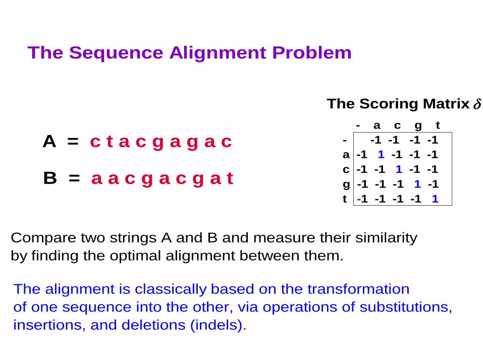
A = c t a c g a g a c
B = a a c g a c g a t
- a c g t
- -1 -1 -1 -1
a -1 1 -1 -1 -1
c -1 -1 1 -1 -1
g -1 -1 -1 1 -1
t -1 -1 -1 -1 1
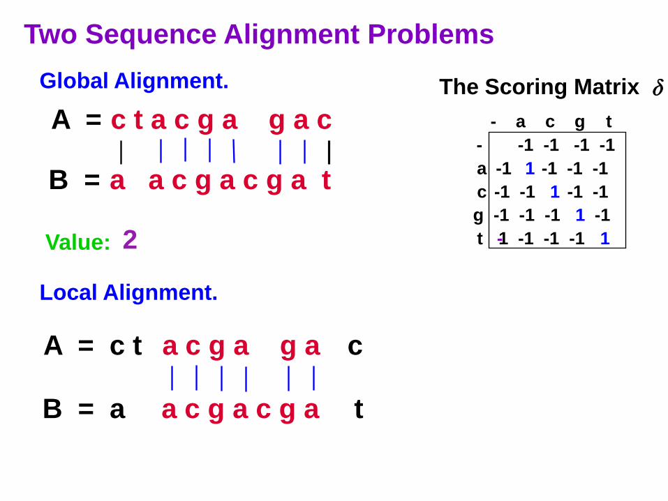
The Sequence Alignment Problem
Compare two strings A and B and measure their similarity
by finding the optimal alignment between them.
The alignment is classically based on the transformation
of one sequence into the other, via operations of substitutions,
insertions, and deletions (indels).
The Scoring Matrix
3
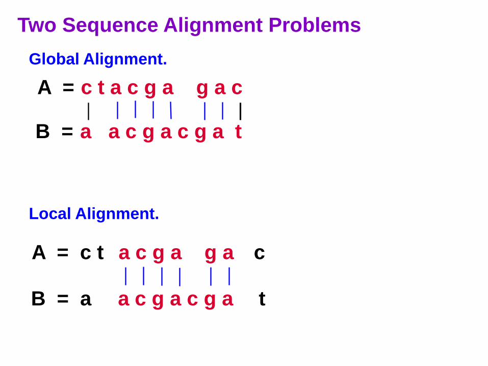
A = c t a c g a g a c
B = a a c g a c g a t
A = c t a c g a g a c
B = a a c g a c g a t
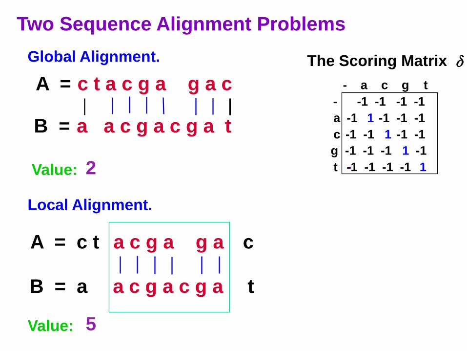
Global Alignment.
Local Alignment.
Two Sequence Alignment Problems
4
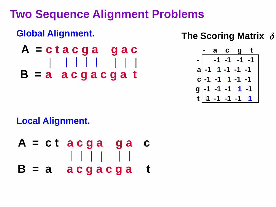
A = c t a c g a g a c
B = a a c g a c g a t
A = c t a c g a g a c
B = a a c g a c g a t
Global Alignment.
Local Alignment.
- a c g t
- -1 -1 -1 -1
a -1 1 -1 -1 -1
c -1 -1 1 -1 -1
g -1 -1 -1 1 -1
t -1 -1 -1 -1 1
The Scoring Matrix
Two Sequence Alignment Problems
5
A = c t a c g a g a c
B = a a c g a c g a t
A = c t a c g a g a c
B = a a c g a c g a t
Global Alignment.
Local Alignment.
- a c g t
- -1 -1 -1 -1
a -1 1 -1 -1 -1
c -1 -1 1 -1 -1
g -1 -1 -1 1 -1
t -1 -1 -1 -1 1
The Scoring Matrix
Two Sequence Alignment Problems
Value: 2
6
A = c t a c g a g a c
B = a a c g a c g a t
A = c t a c g a g a c
B = a a c g a c g a t
Global Alignment.
Local Alignment.
- a c g t
- -1 -1 -1 -1
a -1 1 -1 -1 -1
c -1 -1 1 -1 -1
g -1 -1 -1 1 -1
t --1 -1 -1 -1 1
The Scoring Matrix
Two Sequence Alignment Problems
Value:
Value: 2
5
8
- a c g t
- -1 -1 -1 -1
a -1 1 -1 -1 -1
c -1 -1 1 -1 -1
g -1 -1 -1 1 -1
t -1 -1 -1 -1 1
The Scoring Matrix
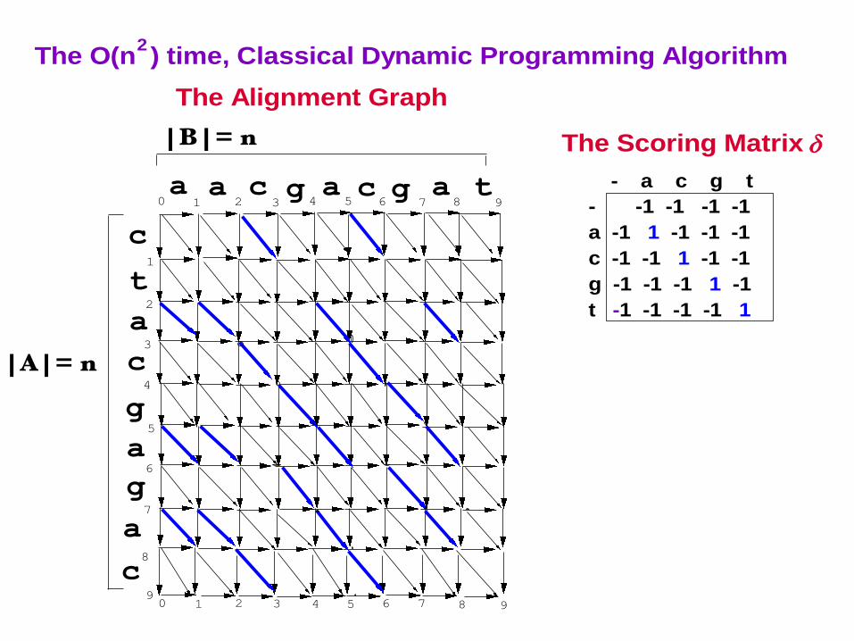
The O(n ) time, Classical Dynamic Programming Algorithm2
c
a
c
t
a a c g a c g a0
1
1 2 3 4 5 6 7 8
2
3
4
a
g
a
g5
6
7
c
|B|= n
|A|= n
t9
9
8
0 1 2 3 4 5 6 8 7 9
The Alignment Graph
9
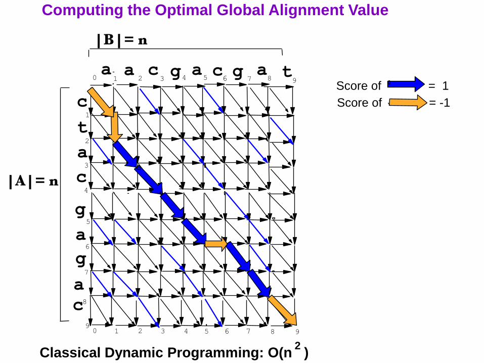
Computing the Optimal Global Alignment Value
c
a
c
t
a a c g a c g a0
1
1 2 3 4 5 6 7 8
2
3
4
a
g
a
g5
6
7
c
|B|= n
|A|= n
t9
9
8
0 1 2 3 4 5 6 8 7 9
Classical Dynamic Programming: O(n )
Score of = 1
Score of = -1
2
10
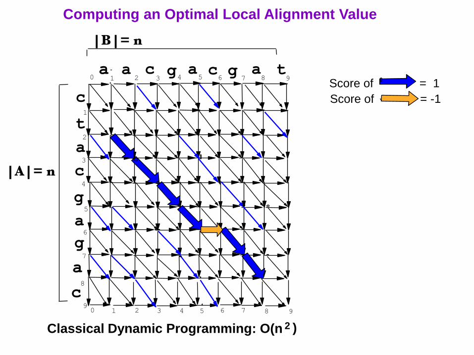
Computing an Optimal Local Alignment Value
c
a
c
t
a a c g a c g a0
1
1 2 3 4 5 6 7 8
2
3
4
a
g
a
g5
6
7
c
|B|= n
|A|= n
t9
9
8
0 1 2 3 4 5 6 8 7 9
Classical Dynamic Programming: O(n )
Score of = 1
Score of = -1
2

11
The O(n ) time, Classical Dynamic Programming Algorithm2
c
a
c
t
a a c g a c g a0
1
1 2 3 4 5 6 7 8
2
3
4
a
g
a
g5
6
7
c
|B|= n
|A|
= n
t9
9
8
0 1 2 3 4 5 6 8 7 9
The Alignment Graph
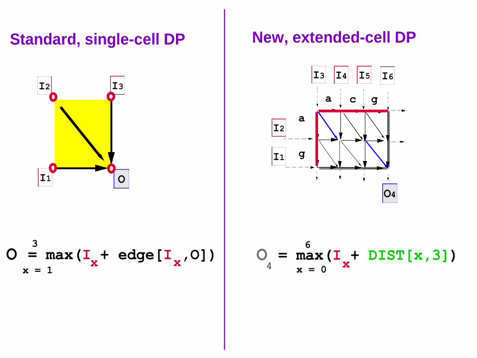
I1
I2 I3
O
O = max(I + edge[I ,O])x
x = 1
3
x
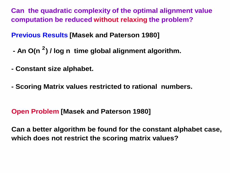
Can the quadratic complexity of the optimal alignment value
computation be reduced without relaxing the problem?
13
Previous Results [Masek and Paterson 1980]
- An O(n ) / log n time global alignment algorithm.
- Constant size alphabet.
- Scoring Matrix values restricted to rational numbers.
Can the quadratic complexity of the optimal alignment value
computation be reduced without relaxing the problem?
2
Open Problem [Masek and Paterson 1980]
Can a better algorithm be found for the constant alphabet case,
which does not restrict the scoring matrix values?
14
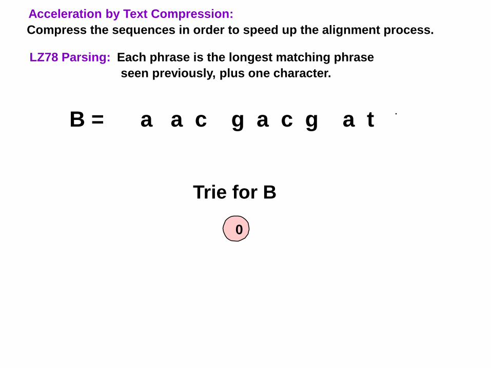
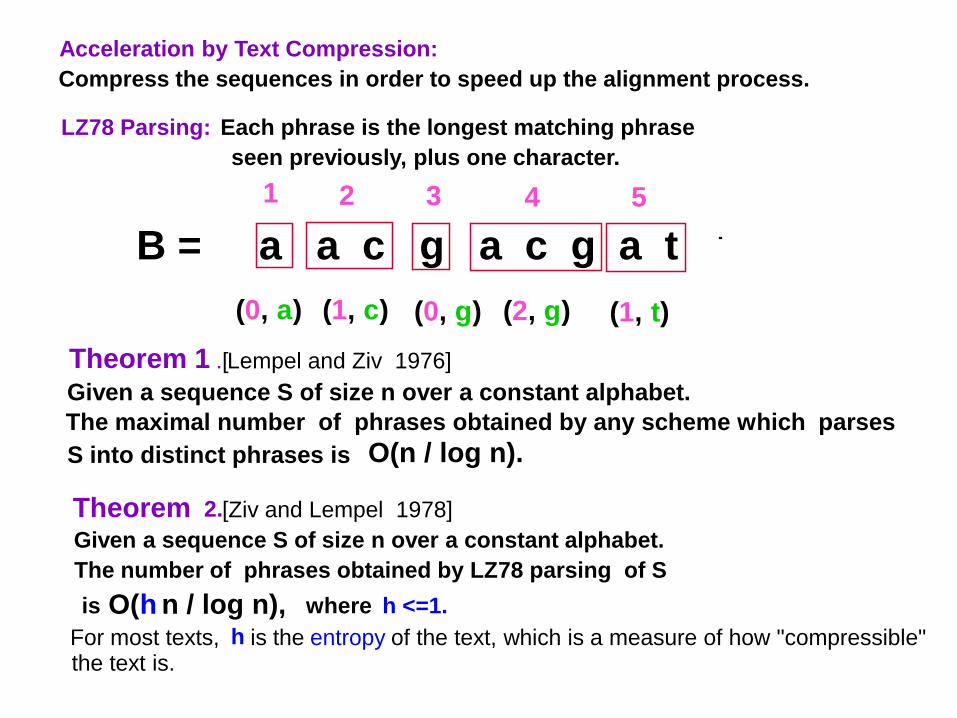
LZ78 Parsing: Each phrase is the longest matching phrase
seen previously, plus one character.
B = a a c g a c g a t
Acceleration by Text Compression:
Compress the sequences in order to speed up the alignment process.
Trie for B
0

15
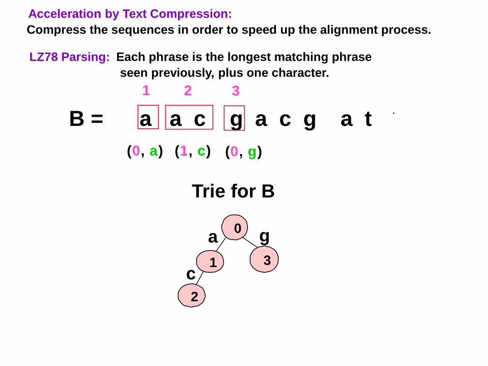
LZ78 Parsing: Each phrase is the longest matching phrase
seen previously, plus one character.
B = a a c g a c g a t
Acceleration by Text Compression:
Compress the sequences in order to speed up the alignment process.
(0, a)
1
Trie for B
0a
1
16
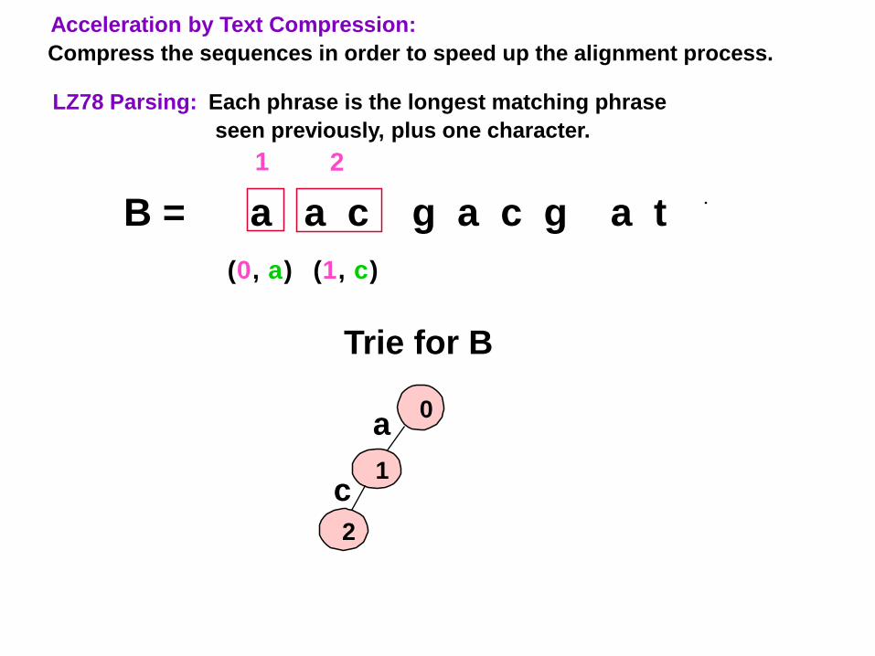
LZ78 Parsing: Each phrase is the longest matching phrase
seen previously, plus one character.
B = a a c g a c g a t
Acceleration by Text Compression:
Compress the sequences in order to speed up the alignment process.
(0, a) (1, c)
1 2
Trie for B
0a
1c
2
17
LZ78 Parsing: Each phrase is the longest matching phrase
seen previously, plus one character.
B = a a c g a c g a t
Acceleration by Text Compression:
Compress the sequences in order to speed up the alignment process.
(0, a) (1, c) (0, g)
1 2 3
Trie for B
0a
1c
2
g
3
18
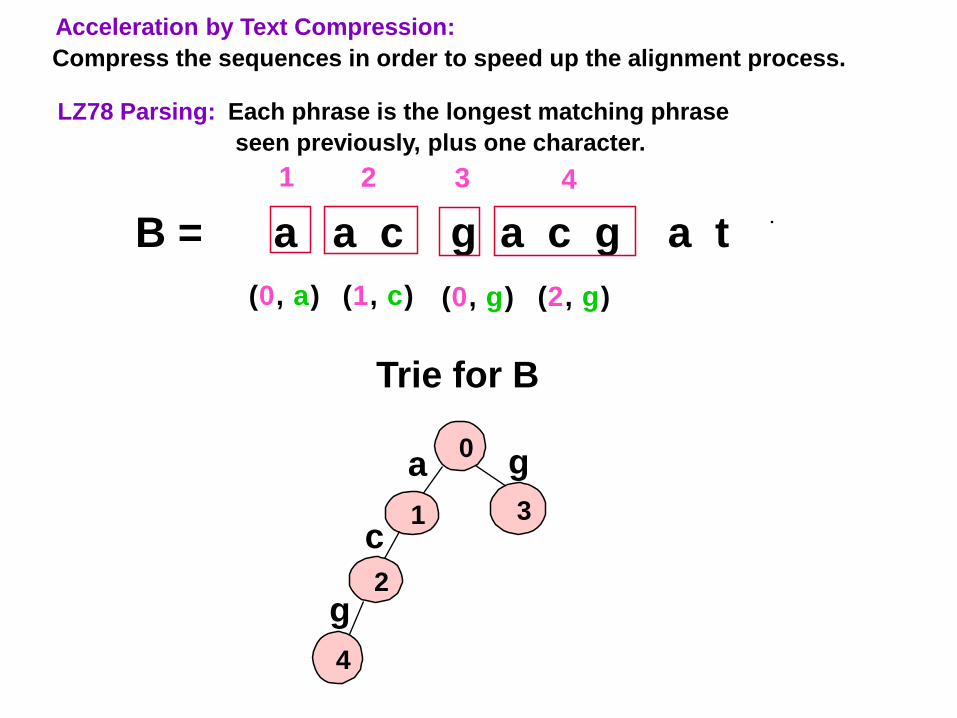
LZ78 Parsing: Each phrase is the longest matching phrase
seen previously, plus one character.
B = a a c g a c g a t
Acceleration by Text Compression:
Compress the sequences in order to speed up the alignment process.
(0, a) (1, c) (0, g) (2, g)
1 2 3 4
Trie for B
0a
1c
2
g
3
g
4
19
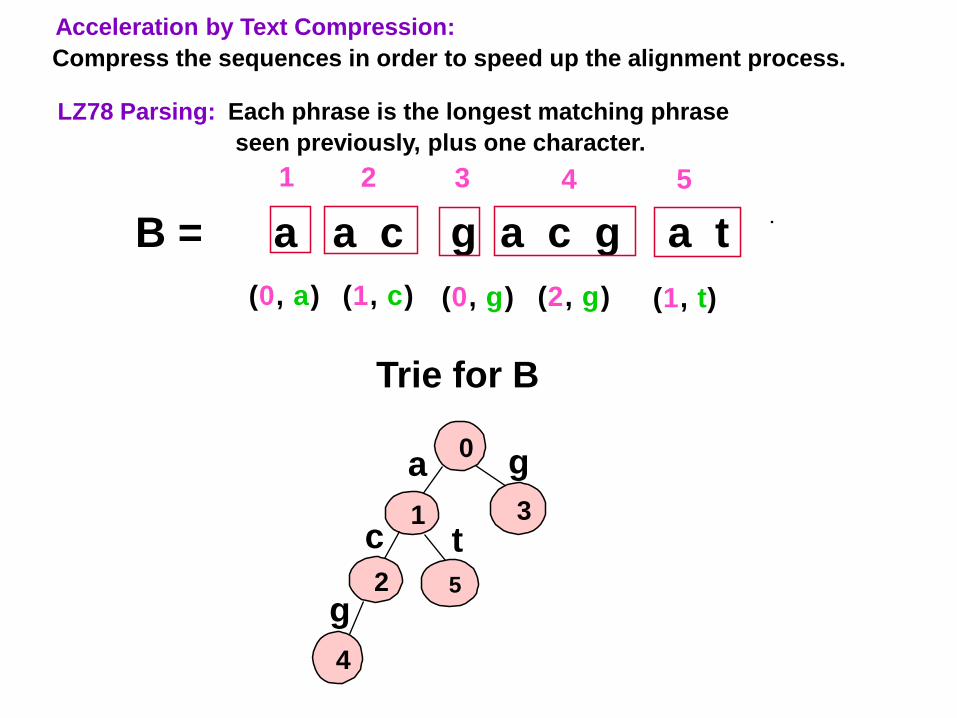
LZ78 Parsing: Each phrase is the longest matching phrase
seen previously, plus one character.
B = a a c g a c g a t
Acceleration by Text Compression:
Compress the sequences in order to speed up the alignment process.
(0, a) (1, c) (0, g) (2, g) (1, t)
1 2 3 4 5
Trie for B
0a
1c
2
g
3
g
4
5
t

Ziv and Lempel
21
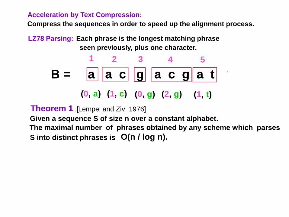
LZ78 Parsing: Each phrase is the longest matching phrase
seen previously, plus one character.
B = a a c g a c g a t
Theorem 1 .[Lempel and Ziv 1976]
Given a sequence S of size n over a constant alphabet.
The maximal number of phrases obtained by any scheme which parses
S into distinct phrases is O(n / log n).
Acceleration by Text Compression:
Compress the sequences in order to speed up the alignment process.
(0, a) (1, c) (0, g) (2, g) (1, t)
1 2 3 4 5
22
LZ78 Parsing: Each phrase is the longest matching phrase
seen previously, plus one character.
B = a a c g a c g a t
Theorem 1 .[Lempel and Ziv 1976]
Given a sequence S of size n over a constant alphabet.
The maximal number of phrases obtained by any scheme which parses
S into distinct phrases is O(n / log n).
Acceleration by Text Compression:
Compress the sequences in order to speed up the alignment process.
(0, a) (1, c) (0, g) (2, g) (1, t)
1 2 3 4 5
Theorem 2.[Ziv and Lempel 1978]
Given a sequence S of size n over a constant alphabet.
The number of phrases obtained by LZ78 parsing of S
is O(h n / log n), where h <=1.
For most texts, h is the entropy of the text, which is a measure of how "compressible" the text is.
24
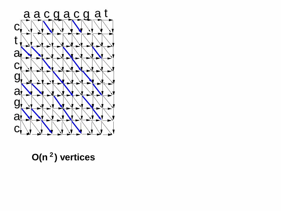
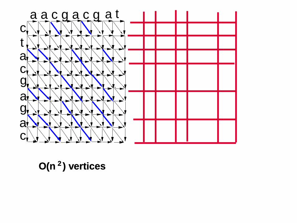
ctacg
ag
a
a a c g a c g
c
O(n ) vertices2
a t
25
ctacg
ag
a
a a c g a c g
c
O(n ) vertices2
a t
26
ctacg
ag
a
a a c g a c g
c
O(n ) vertices2
a t
27
ctacg
ag
a
a a c g a c g
c
O(n ) vertices2 O(n ) vertices2
a t

28
ctacg
ag
a
a a c g a c g
c
O(n ) vertices2
a t
29
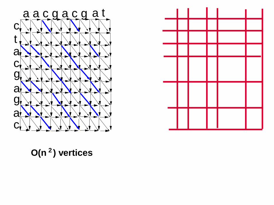
ctacg
ag
a
a a c g a c g
c
O(n ) vertices2
a t
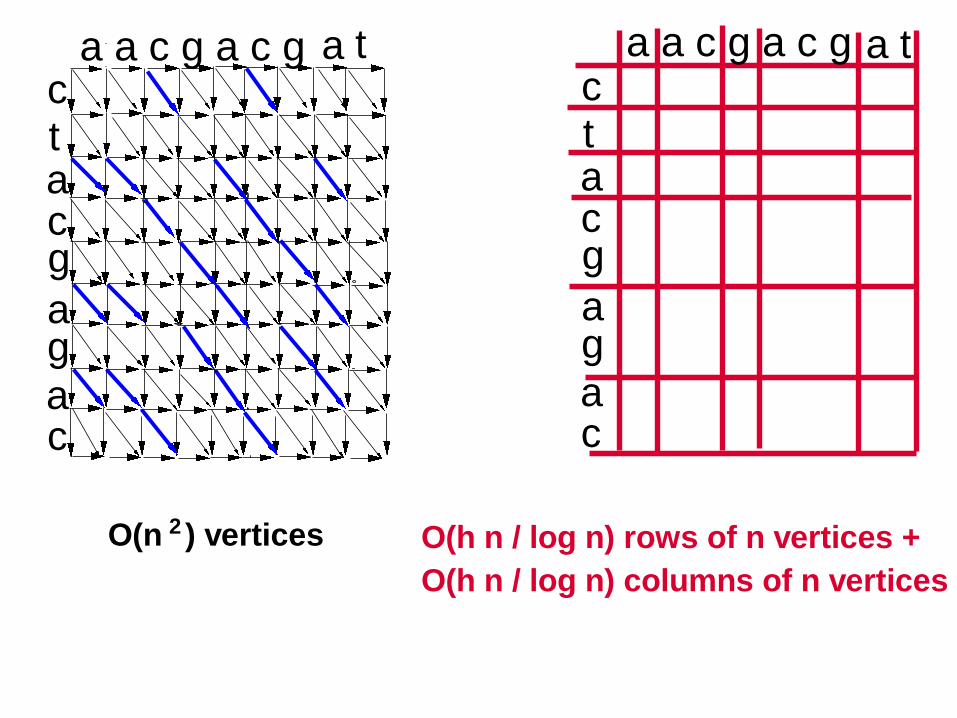
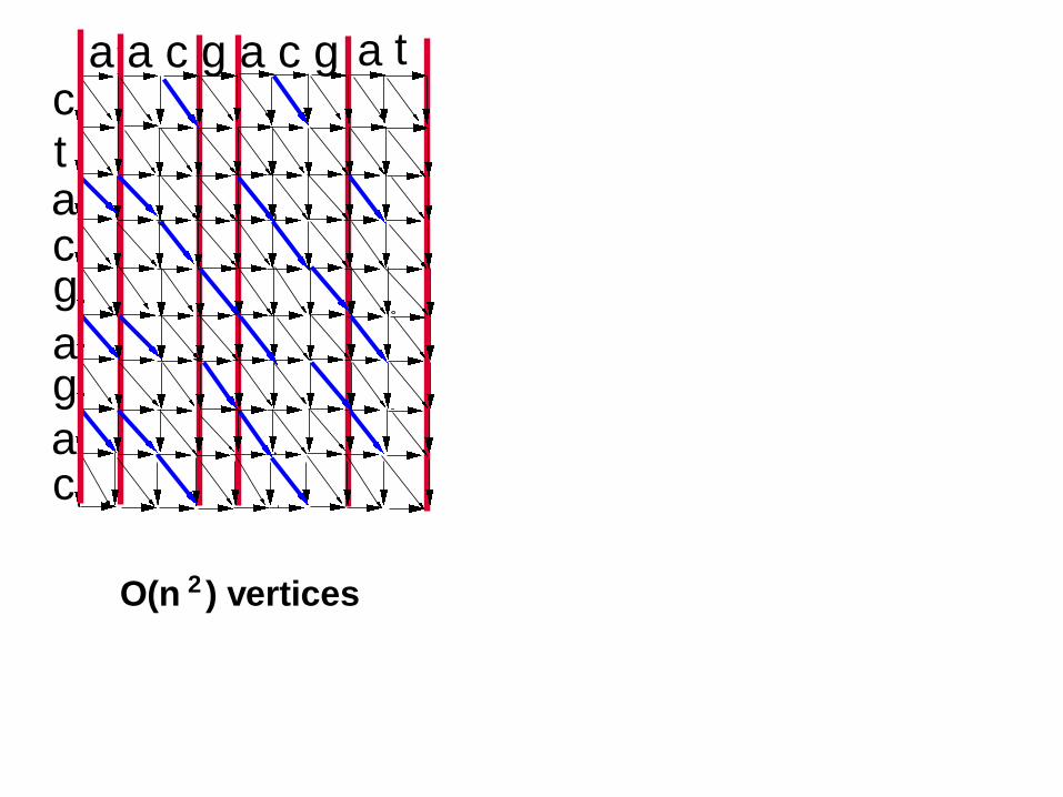
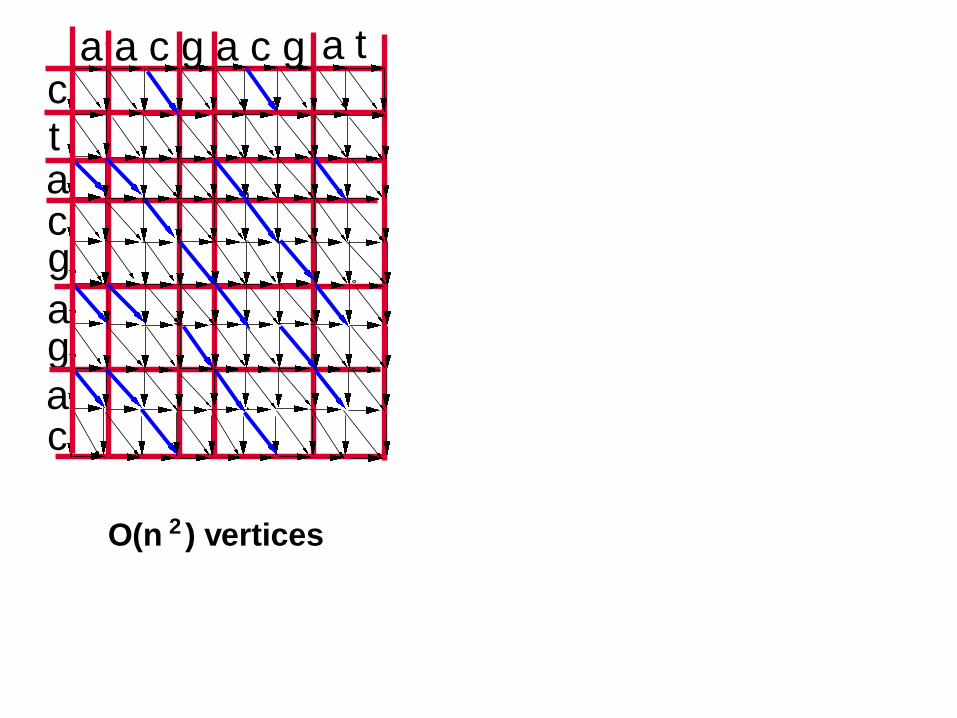
30
ctacg
ag
a
a ta a c g a c g
c
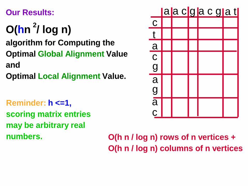
O(h n / log n) rows of n vertices +
O(h n / log n) columns of n vertices
ctacg
ag
a
a a c g a c g
c
O(n ) vertices2
a t

31
ctacg
ag
a
a ta a c g a c g
c
O(h n / log n) rows of n vertices +
O(h n / log n) columns of n vertices
Our Results:
O(hn / log n) algorithm for Computing the
Optimal Global Alignment Value
and
Optimal Local Alignment Value.
2
Reminder: h <=1,
scoring matrix entries
may be arbitrary real
numbers.
32
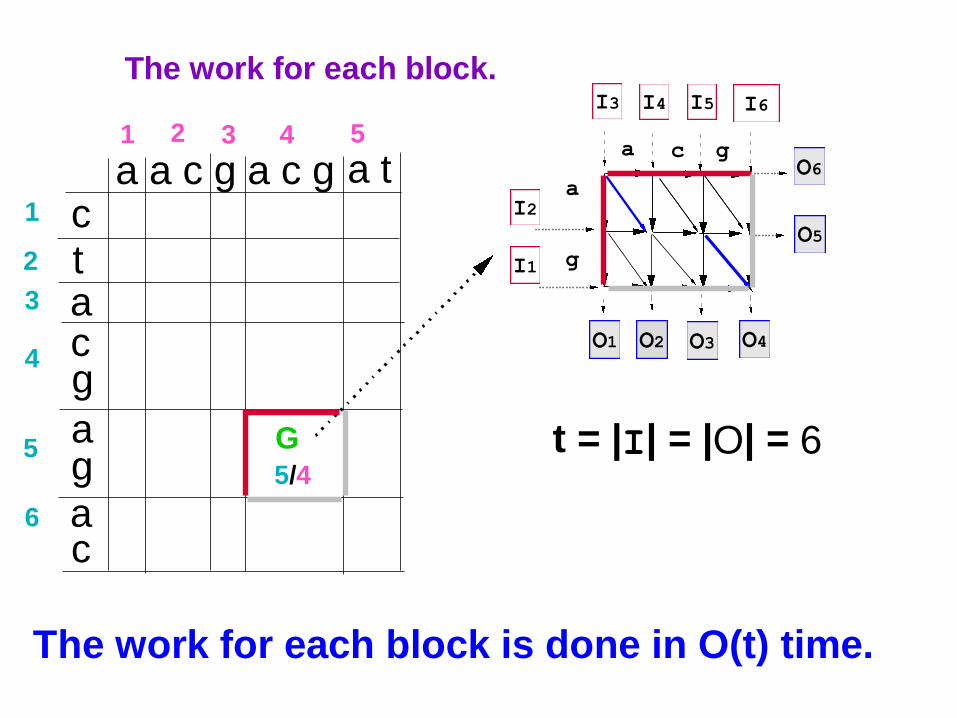
The work for each block.
a a c g a c gctacg
ag
a
a t
5/4
1
1 2 3 4 5
2
3
4
5
6
g
a
ga c
I4 I5 I6I3
I2
I1
O2 O3 O4O1
O6
O5
The work for each block is done in O(t) time.
c
t = |I| = |O| = 6G
33
g
a
ga c
I4 I5 I6I3
I2
I1
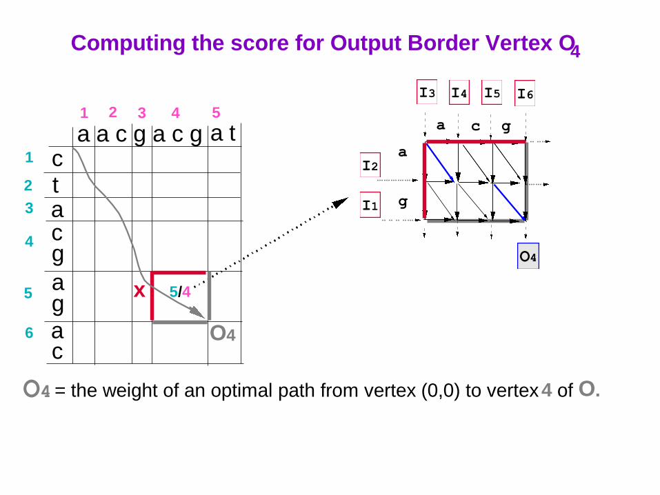
O4
a a c g a c gctacg
ag
a
a t
5/4
1
1 2 3 4 5
2
3
4
5
6
c
O4 = the weight of an optimal path from vertex (0,0) to vertex 4 of O.
O4
Computing the score for Output Border Vertex O4
x
34
g
a
ga c
I4 I5 I6I3
I2
I1
O4
a a c g a c gctacg
ag
a
a t
5/4
1
1 2 3 4 5
2
3
4
5
6
c
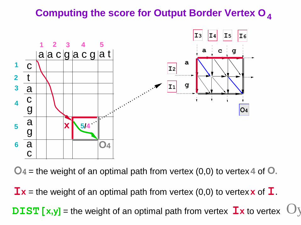
Ix = the weight of an optimal path from vertex (0,0) to vertex x of I.
x
O4 = the weight of an optimal path from vertex (0,0) to vertex 4 of O.
DIST[x,y] = the weight of an optimal path from vertex Ix to vertex O4 .
Computing the score for Output Border Vertex O 4
O4
Oy
35
g
a
ga c
I4 I5 I6I3
I2
I1
O4
a a c g a c gctacg
ag
a
a t1
1 2 3 4 5
2
3
4
5
6
c
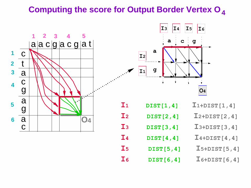
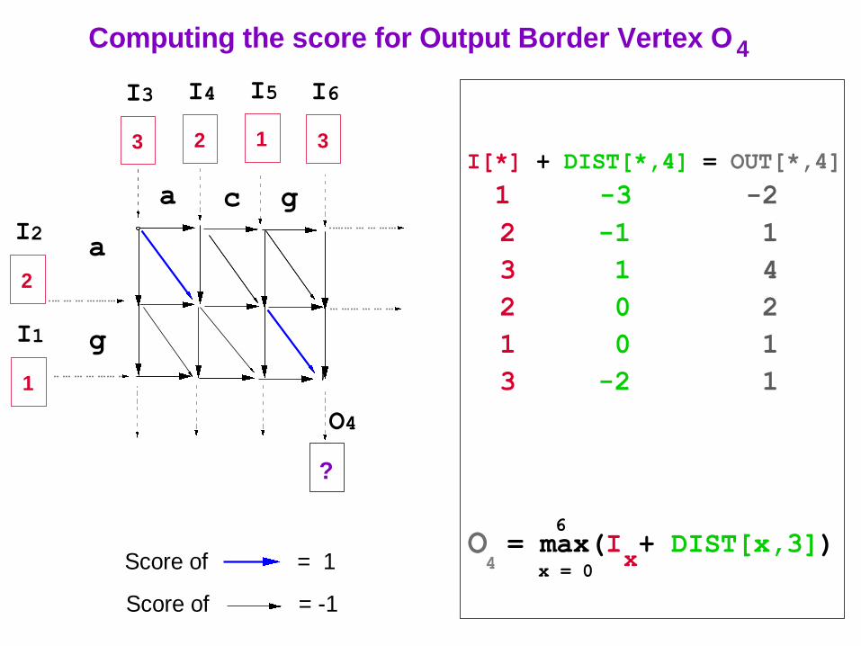
I1 DIST[1,4] I1+DIST[1,4]
I2 DIST[2,4] I2+DIST[2,4]
I3 DIST[3,4] I3+DIST[3,4]
I4 DIST[4,4] I4+DIST[4,4]
I5 DIST[5,4] I5+DIST[5,4]
I6 DIST[6,4] I6+DIST[6,4]
Computing the score for Output Border Vertex O4
O4
36
g
a
ga c
I4 I5 I6I3
I2
I1
O4
a a c g a c gctacg
ag
a
a t1
1 2 3 4 5
2
3
4
5
6
c
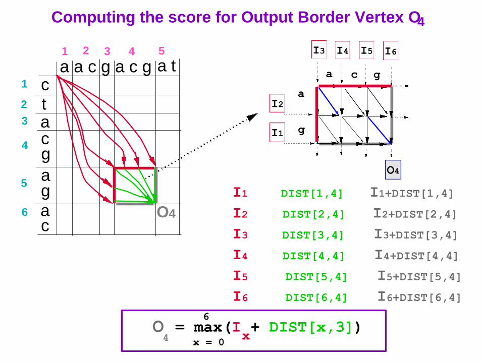
I1 DIST[1,4] I1+DIST[1,4]
I2 DIST[2,4] I2+DIST[2,4]
I3 DIST[3,4] I3+DIST[3,4]
I4 DIST[4,4] I4+DIST[4,4]
I5 DIST[5,4] I5+DIST[5,4]
I6 DIST[6,4] I6+DIST[6,4]
Computing the score for Output Border Vertex O4
O = max(I + DIST[x,3])x 4 x = 0
6
O4
37
g
a
ga c
I4 I5 I6I3
I2
I1
O4
Standard, single-cell DP
I1
I2 I3
O
O = max(I + edge[I ,O])x
x = 1
3
x
O = max(I + DIST[x,3])x 4 x = 0
6
New, extended-cell DP
38
g
a
ga c
3
I3
2
I4
1
I5
3
I6
2
I2
1
I1
O4
?
O = max(I + DIST[x,3])x 4 x = 0
6
Score of = 1
Computing the score for Output Border Vertex O 4
Score of = -1
I[*] + DIST[*,4] = OUT[*,4]
1 -3 -2
2 -1 1
3 1 4
2 0 2
1 0 1
3 -2 1
39
g
a
ga c
3
I3
2
I4
1
I5
3
I6
2
I2
1
I1
O4
?
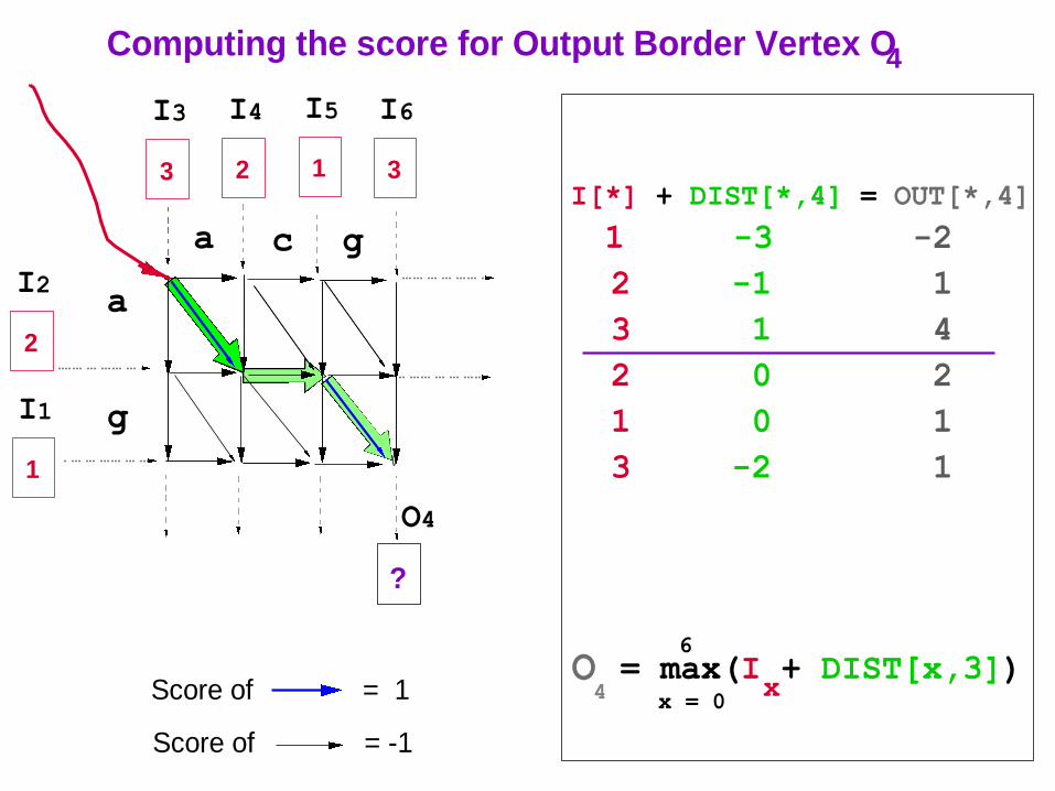
Score of = 1
Computing the score for Output Border Vertex O4
Score of = -1
I[*] + DIST[*,4] = OUT[*,4]
1 -3 -2
2 -1 1
3 1 4
2 0 2
1 0 1
3 -2 1
O = max(I + DIST[x,3])x 4 x = 0
6
40
g
a
ga c
3
I3
2
I4
1
I5
3
I6
2
I2
1
I1
O4
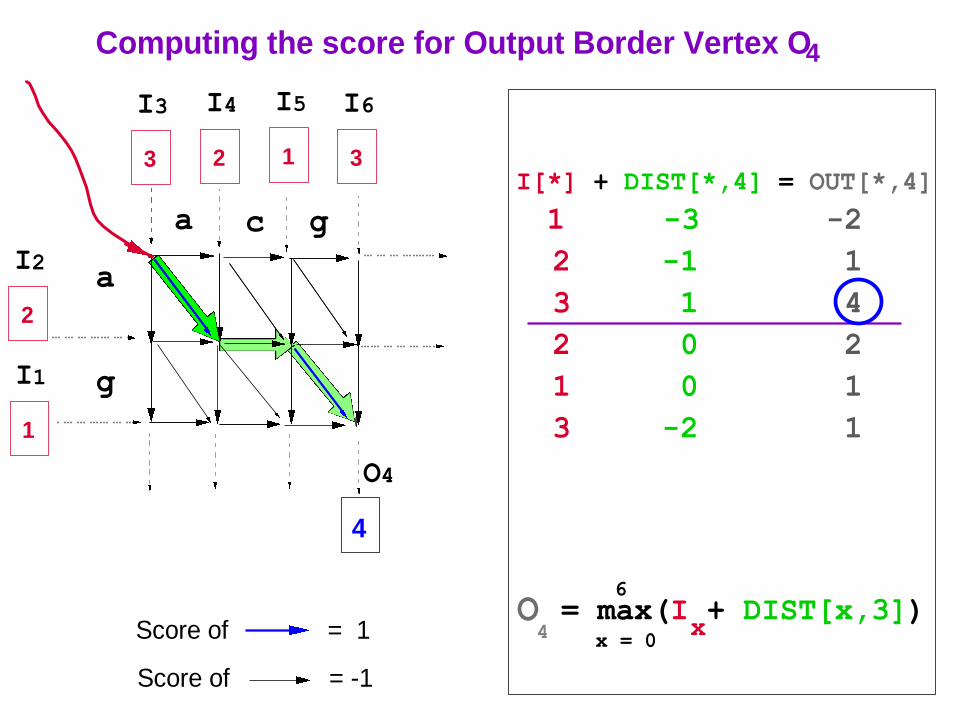
4
Score of = 1
Computing the score for Output Border Vertex O4
Score of = -1
I[*] + DIST[*,4] = OUT[*,4]
1 -3 -2
2 -1 1
3 1 4
2 0 2
1 0 1
3 -2 1
O = max(I + DIST[x,3])x 4 x = 0
6
41
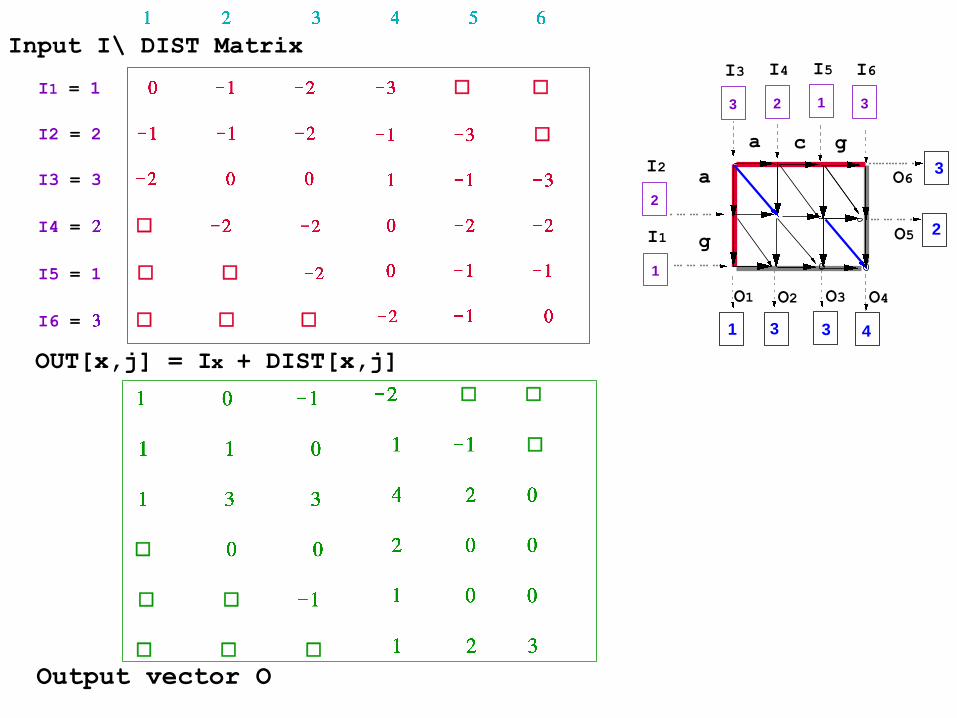
I1 = 1
I2 = 2
I3 = 3
I4 =
I5 = 1
I6 =
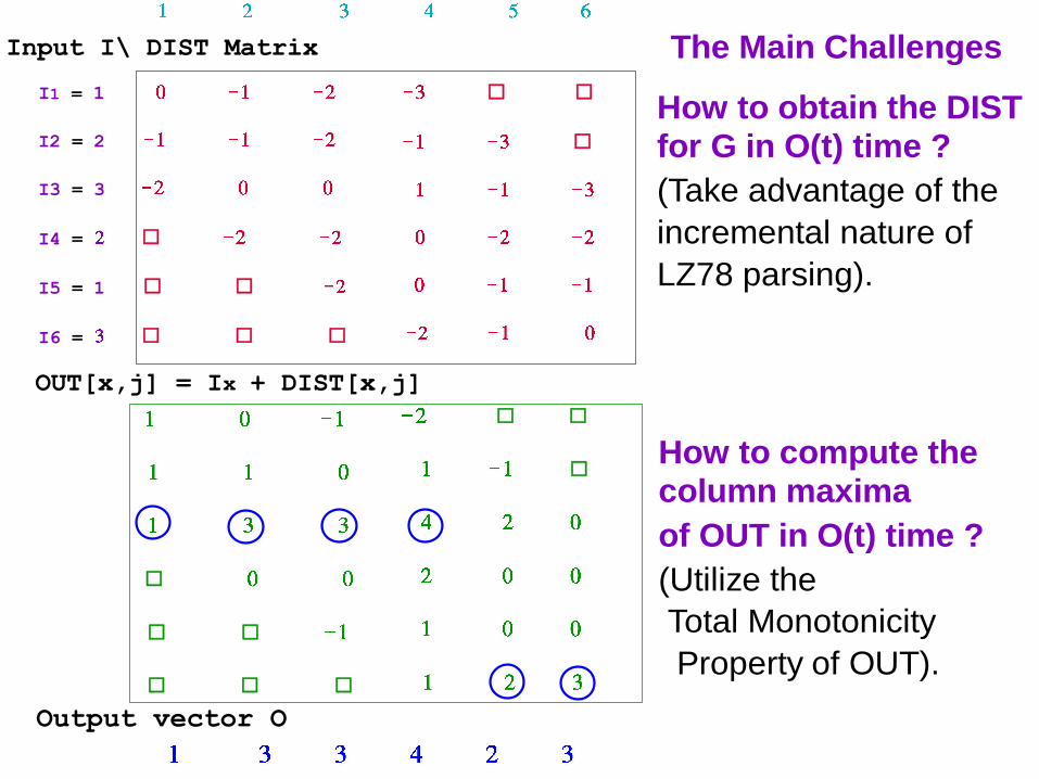
OUT[x,j] = Ix + DIST[x,j]
Input I\ DIST Matrix
Output vector O
g
a
ga c
3
I3
2
I4
1
I5
3
I6
2
I2
1
I1
O2 O4O3
O5
O6
O1
41 3 3
2
3
42
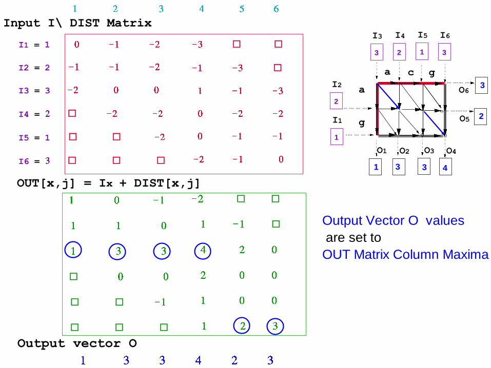
I1 = 1
I2 = 2
I3 = 3
I4 =
I5 = 1
I6 =
OUT[x,j] = Ix + DIST[x,j]
Input I\ DIST Matrix
Output vector O
g
a
ga c
3
I3
2
I4
1
I5
3
I6
2
I2
1
I1
O2 O4O3
O5
O6
O1
41 3 3
2
3
Output Vector O values
are set to
OUT Matrix Column Maxima
43
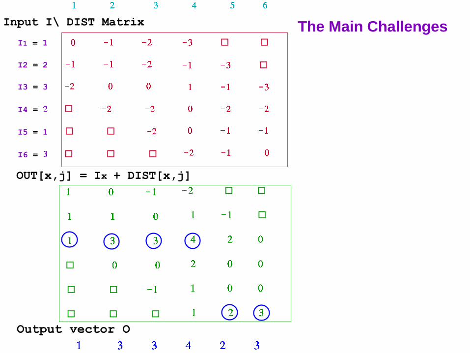
I1 = 1
I2 = 2
I3 = 3
I4 =
I5 = 1
I6 =
OUT[x,j] = Ix + DIST[x,j]
Input I\ DIST Matrix
Output vector O
The Main Challenges
44
I1 = 1
I2 = 2
I3 = 3
I4 =
I5 = 1
I6 =
OUT[x,j] = Ix + DIST[x,j]
Input I\ DIST Matrix
Output vector O
How to compute the
column maxima
of OUT in O(t) time ?
(Utilize the
Total Monotonicity
Property of OUT).
The Main Challenges
45
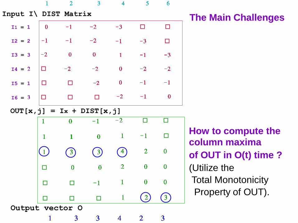
I1 = 1
I2 = 2
I3 = 3
I4 =
I5 = 1
I6 =
OUT[x,j] = Ix + DIST[x,j]
Input I\ DIST Matrix
Output vector O
How to compute the
column maxima
of OUT in O(t) time ?
(Utilize the
Total Monotonicity
Property of OUT).
How to obtain the DIST
for G in O(t) time ?
(Take advantage of the
incremental nature of
LZ78 parsing).
The Main Challenges
46
a
(0,0)
I
O
b
c d
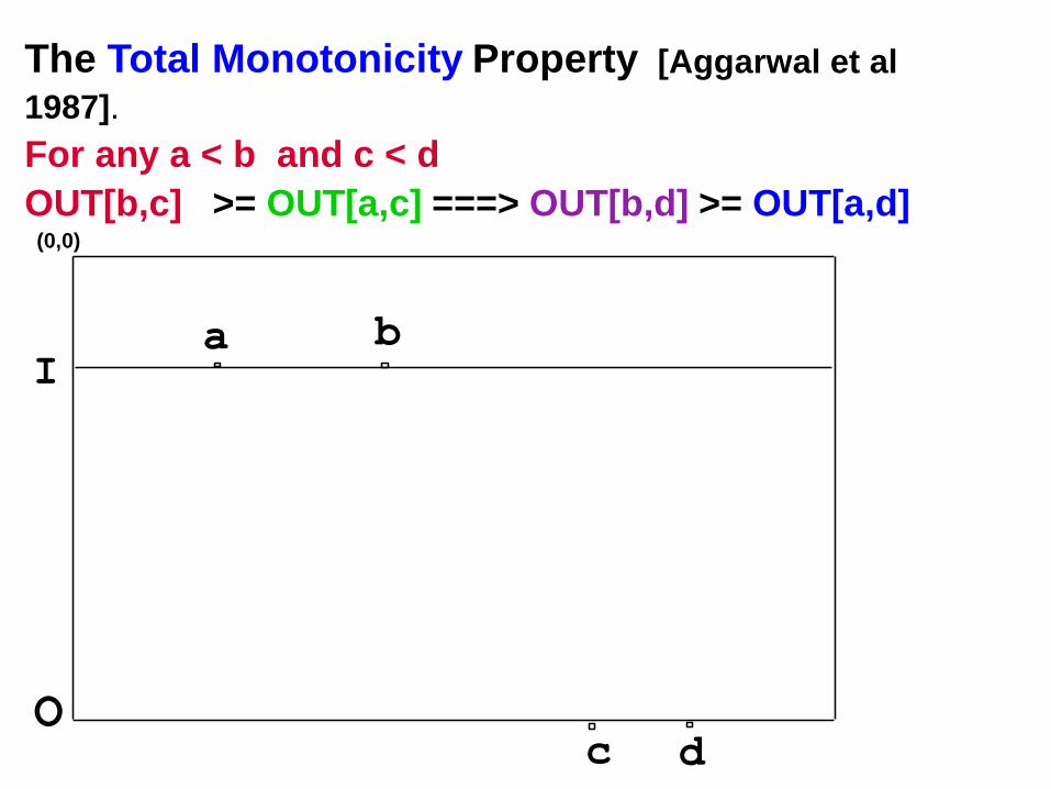
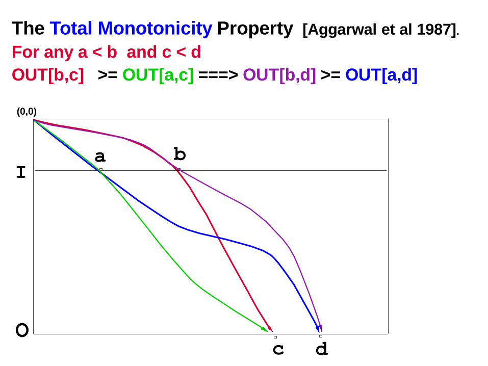
The Total Monotonicity Property [Aggarwal et al
1987].
For any a < b and c < d
OUT[b,c] >= OUT[a,c] ===> OUT[b,d] >= OUT[a,d]
47
a
(0,0)
I
O
b
c d
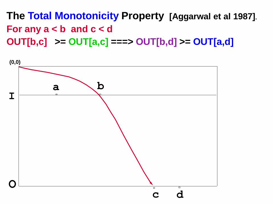
The Total Monotonicity Property [Aggarwal et al 1987].
For any a < b and c < d
OUT[b,c] >= OUT[a,c] ===> OUT[b,d] >= OUT[a,d]

48
a
(0,0)
I
O
b
c d
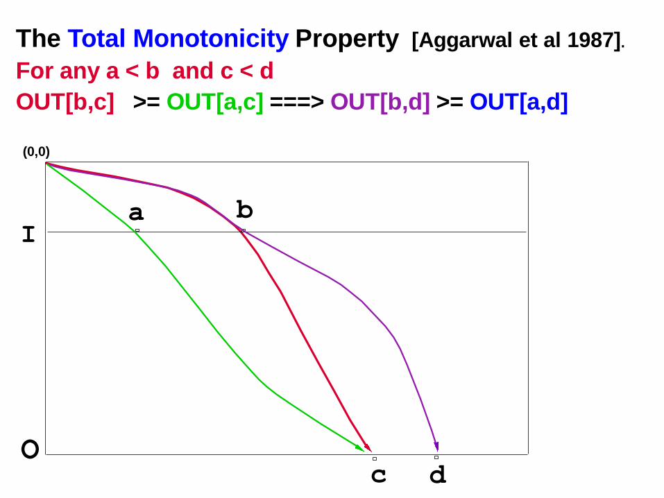
The Total Monotonicity Property [Aggarwal et al 1987].
For any a < b and c < d
OUT[b,c] >= OUT[a,c] ===> OUT[b,d] >= OUT[a,d]
49
a
(0,0)
I
O
b
c d
The Total Monotonicity Property [Aggarwal et al 1987].
For any a < b and c < d
OUT[b,c] >= OUT[a,c] ===> OUT[b,d] >= OUT[a,d]
50
a
(0,0)
I
O
b
c d
The Total Monotonicity Property [Aggarwal et al 1987].
For any a < b and c < d
OUT[b,c] >= OUT[a,c] ===> OUT[b,d] >= OUT[a,d]
51
a
Y
Z
X
W
(0,0)
I
O
b
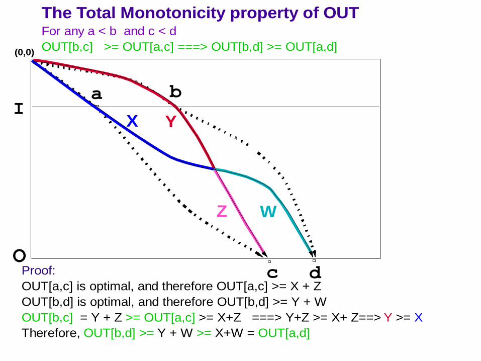
c dProof:
OUT[a,c] is optimal, and therefore OUT[a,c] >= X + Z
OUT[b,d] is optimal, and therefore OUT[b,d] >= Y + W
OUT[b,c] = Y + Z >= OUT[a,c] >= X+Z ===> Y+Z >= X+ Z==> Y >= X
Therefore, OUT[b,d] >= Y + W >= X+W = OUT[a,d]
The Total Monotonicity property of OUTFor any a < b and c < d
OUT[b,c] >= OUT[a,c] ===> OUT[b,d] >= OUT[a,d]
52
a
b
d
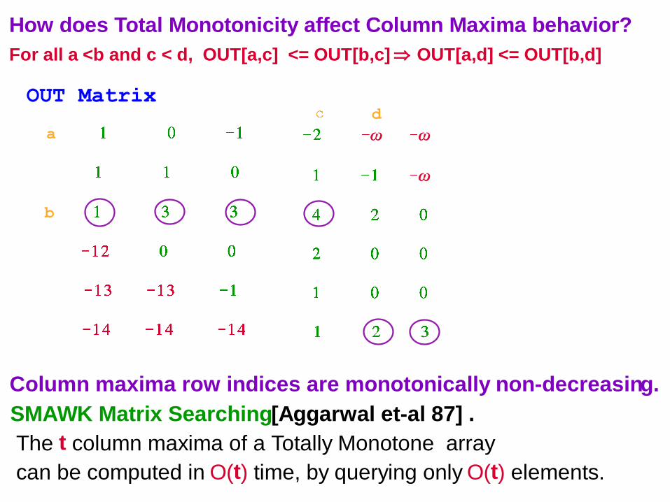
OUT Matrix
How does Total Monotonicity affect Column Maxima behavior?
For all a <b and c < d, OUT[a,c] <= OUT[b,c] OUT[a,d] <= OUT[b,d]
Column maxima row indices are monotonically non-decreasing.
SMAWK Matrix Searching[Aggarwal et-al 87] .
The t column maxima of a Totally Monotone array
can be computed in O(t) time, by querying only O(t) elements.
53
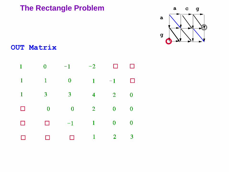
OUT Matrix
The Rectangle Problem
g
a
ga c

54
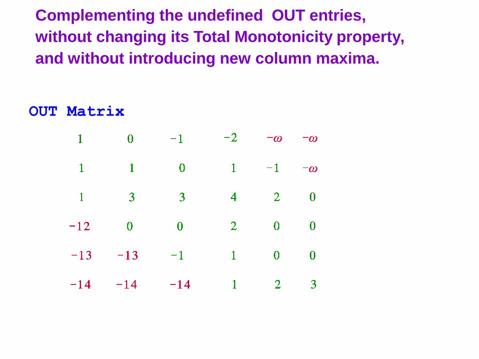
Complementing the undefined OUT entries
(without introducing new column maxima)
1. Upper Right Triangle. All values are set to .
2. Lower Left Triangle.
Let k denote th maximal absolute value of a score in
the scoring matrix .
OUT[i,j] in the lower left triangle will be set to -(n+i+1)*k.
For all a <b and c < d, OUT[a,c] <= OUT[b,c] OUT[a,d] <= OUT[b,d]
55
Complementing the undefined OUT entries,
without changing its Total Monotonicity property,
and without introducing new column maxima.
OUT Matrix

56
I1 = 1
I2 = 2
I3 = 3
I4 =
I5 = 1
I6 =
OUT[x,j] = Ix + DIST[x,j]
Input I\ DIST Matrix
Output vector O
How to compute the
column maxima
of OUT in O(t) time ?
(Utilize the
Total Monotonicity
Property of OUT).
The Main Challenges

57
I1 = 1
I2 = 2
I3 = 3
I4 =
I5 = 1
I6 =
OUT[x,j] = Ix + DIST[x,j]
Input I\ DIST Matrix
Output vector O
How to compute the
column maxima
of OUT in O(t) time ?
(Utilize the
Total Monotonicity
Property of OUT).
How to obtain the DIST
for G in O(t) time ?
(Take advantage of the
incremental nature of
LZ78 parsing).
The Main Challenges
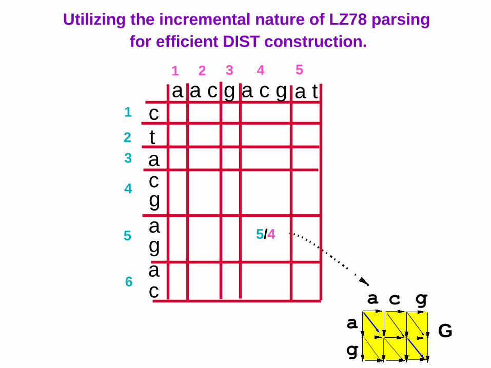
58 G
g
a
ga c
ctacg
ag
a
a t
5/4
1
1 2 3 4 5
2
3
4
5
6
a a c g a c g
c
Utilizing the incremental nature of LZ78 parsing
for efficient DIST construction.
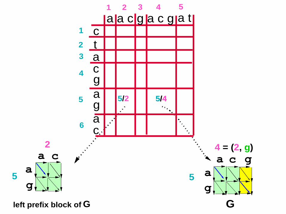
59 left prefix block of G G
g
a
ga c
g
a
a c
ctacg
ag
a
a t
5/4
1
1 2 3 4 5
2
3
4
5
6
a a c g a c g
c
5/2
4 = (2, g)
5/4
55
2
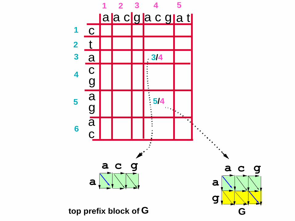
60 G
g
a
ga c
a
3/4
ctacg
ag
a
a t
5/4
1
1 2 3 4 5
2
3
4
5
6
a a c g a c g
c
top prefix block of G
ga c
61
3/4
5/2
3/2
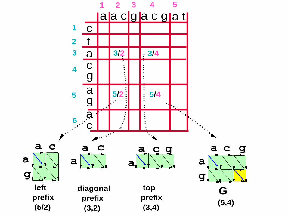
left
prefix
(5/2)
diagonal
prefix
(3,2)
top
prefix
(3,4)
G (5,4)
g
a
ga cga c
g
a
a c
a
a c
a
ctacg
ag
a
a t
5/4
1
1 2 3 4 5
2
3
4
5
6
a a c g a c g
c
62
3/43/2
g
a
ga c ga c
g
a
a c
a
ctacg
ag
a
a t
5/4
1
1 2 3 4 5
2
3
4
5
6
a a c g a c g
c
-3
-1
1
0
0
-2
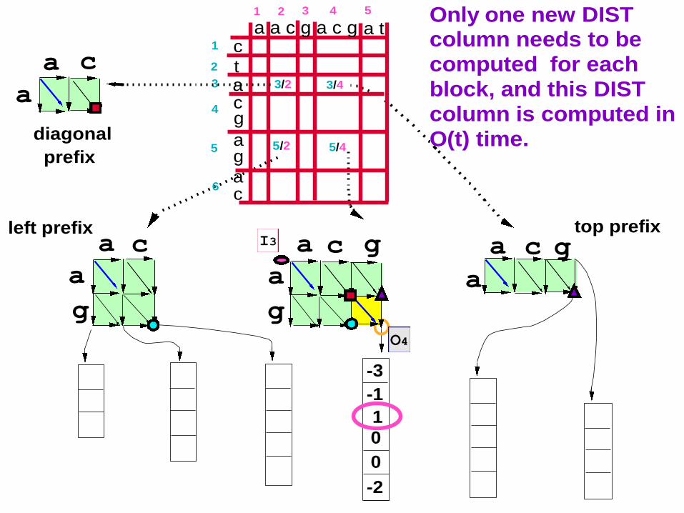
Only one new DIST column needs to be
computed for each
block, and this DIST
column is computed in
O(t) time.diagonal
prefix
a
a c
5/2
left prefix
left prefix
top prefix
I3
O4
63
3/4
5/2
3/2
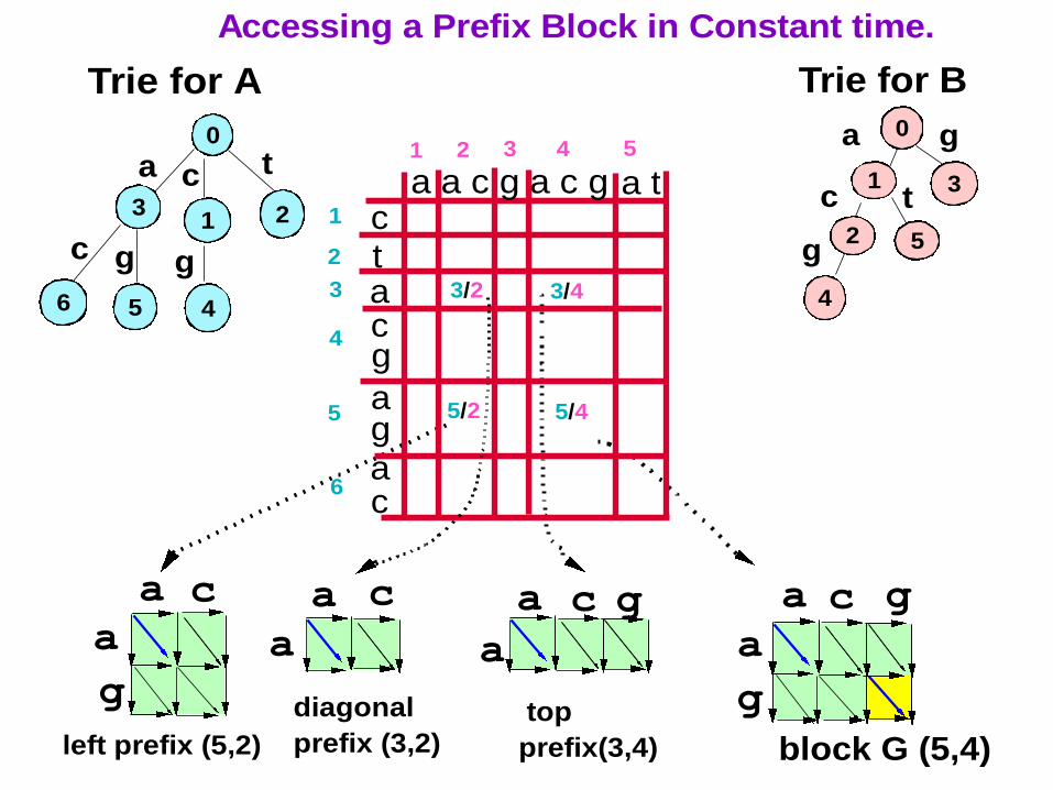
left prefix (5,2)
diagonal
prefix (3,2)
top
prefix(3,4)
block G (5,4)
g
a
ga cga c
g
a
a c
a
a c
a
ctacg
ag
a
a t
5/4
1
1 2 3 4 5
2
3
4
5
6
a a c g a c g
c
Accessing a Prefix Block in Constant time.
a c
Trie for A
0
13
5
2
t
4
gg
a
c
g
g
Trie for B
0
31
2
46
5c
t
Presentation
• R89922024 蘇展弘
• B86202049 葉恆青
• R90725054 呂育恩
• R90922001 張文亮
• R90922091 游騰楷
Trie for A
0
31
2
54
g
c
ta
g
Trie for B
0
1 3
2
4
g
ga
c
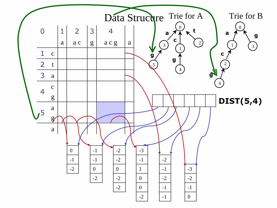
DIST(5,4)
-3
-1
1
0
0
-2
-2
-2
0
-2
-2
-1
-1
0
-2
0
-1
-2
-2
-1
-2
-1
-1
-3
-2
-1
0
0 1 2 3 4
a a c g a c g a
1 c
2 t
3 a
4c
g
5a
g
a
Data Strucure
Trie for A
0
31
2
54
g
c
ta
g
Trie for B
0
1 3
2
4
g
ga
c
DIST(5,4)
-3
-1
1
0
0
-2
-2
-2
0
-2
-2
-1
-1
0
-2
0
-1
-2
-2
-1
-2
-1
-1
-3
-2
-1
0
0 1 2 3 4
a a c g a c g a
1 c
2 t
3 a
4c
g
5a
g
a
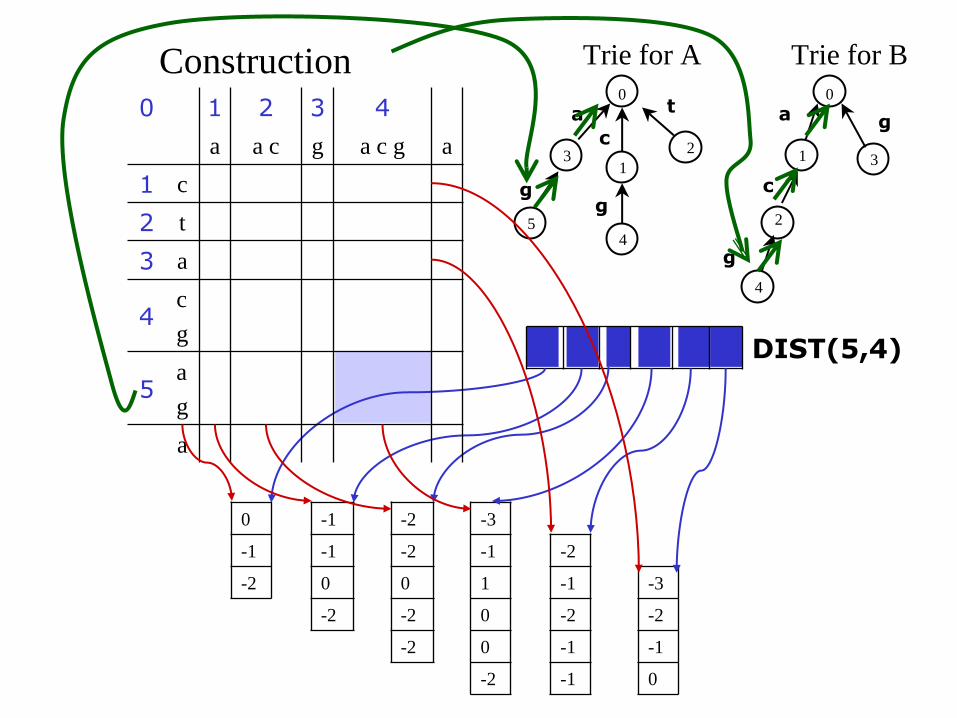
Construction
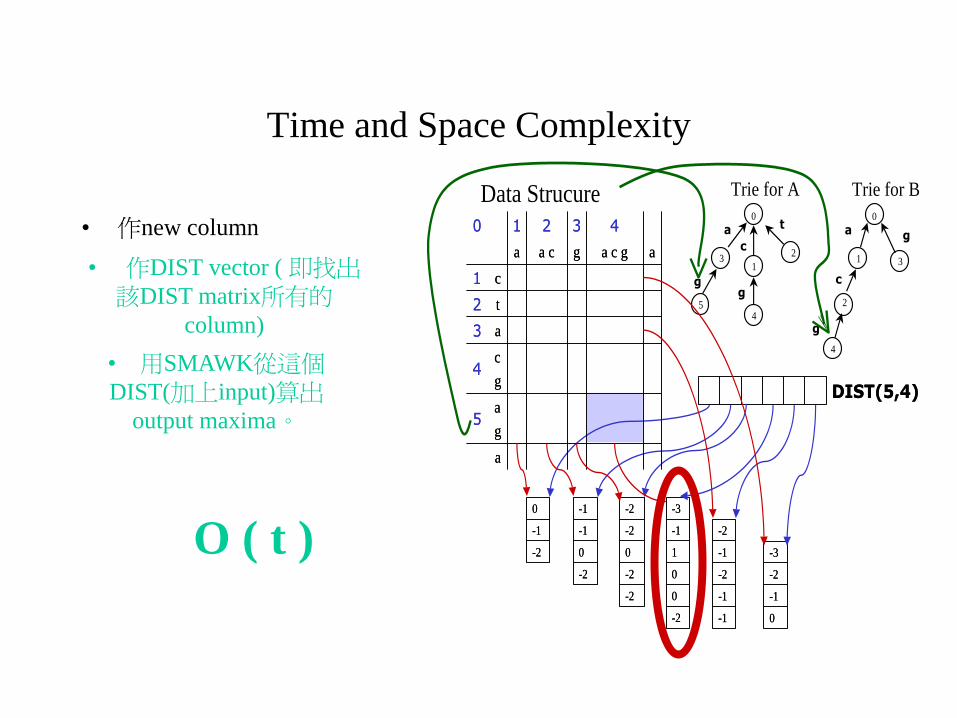
Time and Space Complexity
• 作new column
Trie for A
0
31
2
54
g
c
ta
g
Trie for B
0
1 3
2
4
g
ga
c
DIST(5,4)DIST(5,4)
-2
0
0
1
-1
-3
-2
0
0
1
-1
-3
-2
-2
0
-2
-2
-2
-2
0
-2
-2
-2
0
-1
-1
-2
0
-1
-1
-2
-1
0
-2
-1
0
-1
-1
-2
-1
-2
-1
-1
-2
-1
-2
0
-1
-2
-3
0
-1
-2
-3
a
a
g5
c
g4
a3
t2
c1
aa c gga ca
43210
a
a
g5
c
g4
a3
t2
c1
aa c gga ca
43210
Data Strucure
• 作DIST vector ( 即找出該DIST matrix所有的
column)
• 用SMAWK從這個DIST(加上input)算出
output maxima。
O ( t )

68
ctacg
ag
a
a ta a c g a c g
c
O(h n / log n) rows of n vertices +
O(h n / log n) columns of n vertices
ctacg
ag
a
a a c g a c g
c
O(n ) vertices2
a t
69
ctacg
ag
a
a ta a c g a c g
c
O(h n / log n) rows of n vertices +
O(h n / log n) columns of n vertices
Our Results:
O(hn / log n) algorithm for Computing the
Optimal Global Alignment Value
and
Optimal Local Alignment Value.
2
Reminder: h <=1,
scoring matrix entries
may be arbitrary real
numbers.

70
I1 = 1
I2 = 2
I3 = 3
I4 =
I5 = 1
I6 =
OUT[x,j] = Ix + DIST[x,j]
Input I\ DIST Matrix
Output vector O
How to compute the
column maxima
of OUT in O(t) time ?
(Utilize the
Total Monotonicity
Property of OUT).
How to obtain the DIST
for G in O(t) time ?
(Take advantage of the
incremental nature of
LZ78 parsing).
The Main Challenges
71
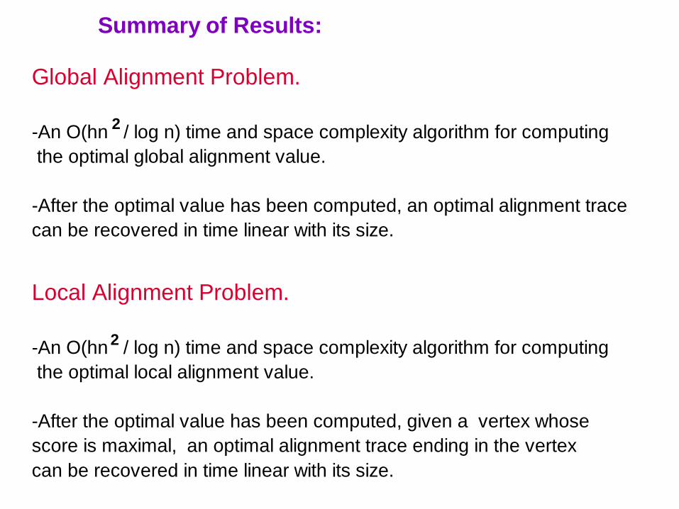
Summary of Results:
Global Alignment Problem.
-An O(hn / log n) time and space complexity algorithm for computing
the optimal global alignment value.
-After the optimal value has been computed, an optimal alignment trace
can be recovered in time linear with its size.
Local Alignment Problem.
-An O(hn / log n) time and space complexity algorithm for computing
the optimal local alignment value.
-After the optimal value has been computed, given a vertex whose
score is maximal, an optimal alignment trace ending in the vertex
can be recovered in time linear with its size.
2
2
72
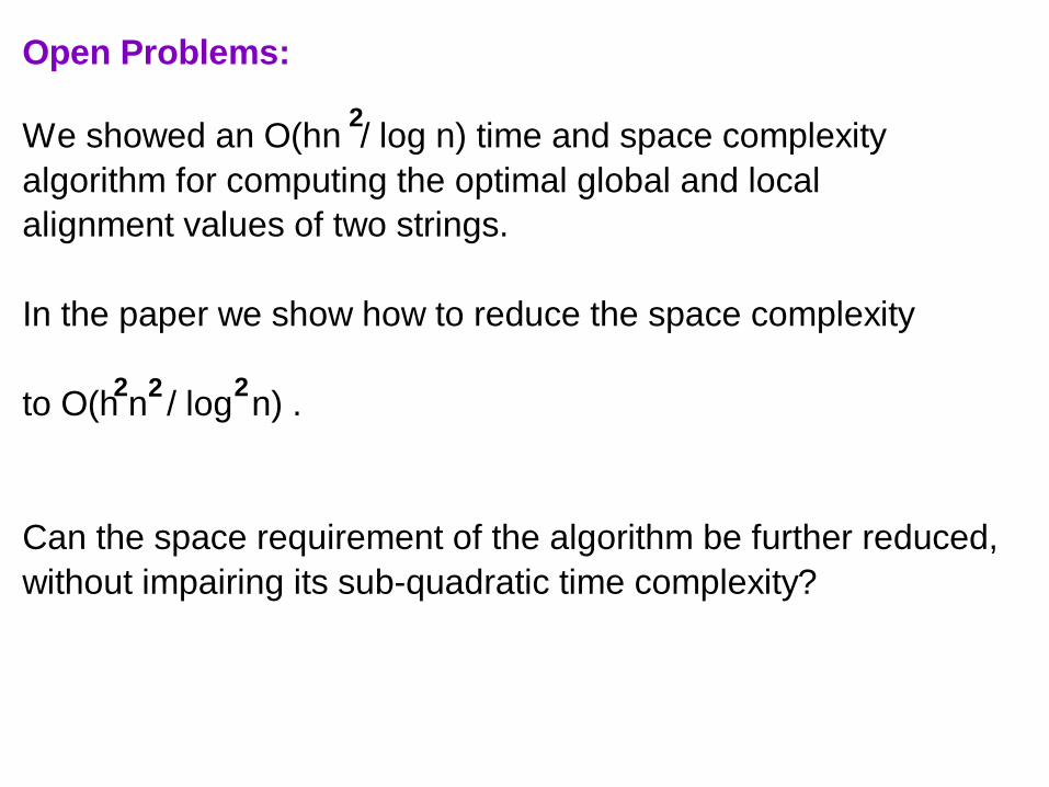
Open Problems:
We showed an O(hn / log n) time and space complexity
algorithm for computing the optimal global and local
alignment values of two strings.
In the paper we show how to reduce the space complexity
to O(h n / log n) .
Can the space requirement of the algorithm be further reduced,
without impairing its sub-quadratic time complexity?
2
2 2 2

73
Thank You !