1

Sequential Convolutional Recurrent NeuralNetworks for Fast Automatic Modulation

ClassificationKaisheng Liao, Guanhong Tao, Yi Zhong, Yaping Zhang, and Zhenghong Zhang

Abstract—A novel and efficient end-to-end learning modelfor automatic modulation classification (AMC) is proposed forwireless spectrum monitoring applications, which automaticallylearns from the time domain in-phase and quadrature (IQ) datawithout requiring the design of hand-crafted expert features.With the intuition of convolutional layers with pooling servingas front-end feature distillation and dimensionality reduction,sequential convolutional recurrent neural networks (SCRNNs)are developed to take complementary advantage of parallelcomputing capability of convolutional neural networks (CNNs)and temporal sensitivity of recurrent neural networks (RNNs).Experimental results demonstrate that the proposed architec-ture delivers overall superior performance in signal to noiseratio (SNR) range above -10 dB, and achieves significantlyimproved classification accuracy from 80% to 92.1% at highSNRs, while drastically reduces the training and prediction timeby approximately 74% and 67%, respectively. Furthermore, acomparative study is performed to investigate the impacts ofvarious SCRNN structure settings on classification performance.A representative SCRNN architecture with the two-layer CNNand subsequent two-layer long short-term memory (LSTM) isdeveloped to suggest the option for fast AMC.

Index Terms—deep learning, convolutional neural networks,recurrent neural networks, automatic modulation classification,spectrum monitoring, cognitive radio.

I. INTRODUCTION

W IRELESS spectrum monitoring over time, space andfrequency is important for effective use of the scarce

spectral resources in various commercial areas [1]–[5]. As anintegral part of wireless spectrum monitoring systems, auto-matic modulation classification (AMC) is used to recognizemodulation types without prior knowledge of the received sig-nals and channel parameters [6]–[8]. AMC has been proven tobe an essential capability for transmitter identification, wirelessspectrum anomaly detection and radio environment awareness.It improves radio spectrum utilization and opens the possibilityof intelligent decision for context-aware autonomous wirelessspectrum monitoring systems.

Traditional AMC approaches discussed in literature can beroughly brought down into two main categories: likelihood-based approaches and feature-based approaches [9], [10]. Thelikelihood-based approaches utilize hypothesis testing theoryand form a judgment criterion by analyzing statistical charac-teristics of signals [11], [12]. In likelihood-based approaches,modulation classification is framed as Bayesian estimation tooptimize the probability of classification. However, approachesof this type are not robust in the presence of unknownchannel conditions and suffer from heavy computational load

on their practical implementations. Traditional feature-basedapproaches mainly focus on expert feature extraction and clas-sification criteria [13]–[18]. They utilize expert features suchas higher order cyclic moments for modulation classification.It is easy and simple for these approaches to be implementedin practical systems. However, hand-crafting expert featuresand hard-coding rules for modulation classification make itdifficult to scale to new modulation types in non-cooperativescenarios.

Recently, researchers in wireless communications havestarted to apply deep neural networks to cognitive radiotasks with some success [19]–[32]. The authors in [19],[24] demonstrated that convolutional neural networks (CNNs)trained on time domain in-phase and quadrature (IQ) datasignificantly outperform conventional expert feature-based ap-proaches. The authors in [20], [23] utilized recurrent neuralnetworks (RNNs) for learning temporal representations toachieve higher classification accuracy than that of the CNNsintroduced in [19]. In [21], the authors directly adopted con-volutional long short-term deep neural networks (CLDNNs)from voice processing domain. The authors in [33] developeda data-driven fusion method to obtain better classificationaccuracy using the combination of the two CNNs trained ondifferent datasets. Ramjee et al. [32] performed a comparativestudy of various typical deep neural networks and reduced thetraining complexity by reducing the input dimensionality withsubsampling techniques.

In autonomous wireless spectrum monitoring systems, on-line learning is fundamental for accommodating new emergingmodulation types and complex environmental circumstances.However, those RNN models delivering high classification ac-curacy suffer from computational complexity and long trainingtime. In this work, we develop a novel and efficient sequentialconvolutional recurrent neural network (SCRNN) architecturecombining parallel computing capability of CNNs with tempo-ral sensitivity of RNNs. Experimental results demonstrate thatour approach outperforms the state-of-the-art on classificationperformance, while significantly improves the rate of conver-gence compared with the pure CNN and RNN architectures.The code and datasets for all the deep learning models willmade public soon for future research.1

The rest of the paper is organized as follows. In SectionII, an overview of the modulation benchmark dataset is intro-duced, and the two baseline models are briefly explained. The

1https://github.com/kython

arX

iv:1

909.

0305

0v1

[ee

ss.S

P] 9

Sep

201

9

2

TABLE IBENCHMARK DATASET PARAMETERS.

Dataset RadioML2016.10a

Modulations

8 Digital Modulations: BPSK,QPSK, 8PSK, 16QAM, 64QAM,BFSK, CPFSK, and PAM43 Analog Modulations: WBFM,AM-SSB, and AM-DSB

Length per sample 128

Signal format In-phase and quadrature (IQ)

Signal dimension 2×128 per Sample

Duration per sample 128 µs

Sampling frequency 1 MHz

Samples per symbol 8

SNR Range [-20 dB, -18 dB, -16 dB, . . ., 18 dB]

Total number of samples 220000 vectors

Number of training samples 198000 vectors

Number of test samples 22000 vectors

proposed model and the parameters used for training alongwith other implementation details are clearly stated in SectionIII. Section IV details the classification results and discussesthe advantages of the proposed model. Conclusions and futurework are presented in Section V.

II. DATASET AND BASELINES

A. Dataset

In a wireless spectrum monitoring system, the receivedsignal can be typically represented as:

r(t) = s(t) ∗ h(t) + n(t) (1)

where s(t) denotes the noise free complex baseband en-velope of the received signal, and h(t) refers to the timevarying impulse response of the transmitted wireless channel.n(t) represents the additive white Gaussian noise (AWGN)reflecting thermal noise. The complex received signal r(t) iscommonly sampled in IQ format due to its simplicity.

A typical modulation dataset RadioML2016.10a generatedby GNU Radio is used as the benchmark dataset for trainingand evaluating the performance of the proposed architecture,similar as the MNIST dataset in the vision domain [34]. Thedataset follows the signal representation as given in equation 1.Detailed parameter description of the dataset is shown in TableI. Radio channel effects are relatively well characterized in thedataset. Chanel imperfections such as multi-path fading, ran-dom walk drifting of carrier frequency oscillator and sampletime clocks, AWGN, along with unknown scale, translation,and dilation transformation are introduced into the signal inthe dataset for reflecting the real electromagnetic environment[34]. The dataset is labeled with both SNR ground truth andmodulation types.

B. Baselines

The two models are chosen as the baselines for furthercomparisons due to their results showing the significant im-

Fig. 1. Schematic diagram of the (a) convolutional neural network (CNN)baseline model, (b) long short-term memory (LSTM) baseline model, and (c)proposed sequential convolutional recurrent neural network (SCRNN) model.

provements upon expert feature-based approaches. Any furtherimprovements should be considered state-of-the-art.

One is the CNN architecture proposed by O’shea et al.[19]. As shown in Fig. 1(a), the baseline model is a 4-layer network made up of two convolutional layers and twodense layers. Each hidden layer utilizes rectified linear unit(ReLU) activation functions and dropout of 50% except for asoftmax activation function on the one-hot output layer. Theadam optimizer and categorical cross entropy loss function areapplied to the base model.

The other baseline model is proposed by Rajendran et al.[23], shown in Fig. 1(b). The model is comprised of two 128-unit long short-term memory (LSTM) layers and an 11-unitdense layer with a softmax activation. The first LSTM layerreturns the full sequences while the second one just returns thelast state. The dropout is also adopted to reduce overfitting.The adam optimizer and categorical cross entropy loss functionare applied to the model. Note that this model learns fromthe time domain information of the modulation schemes usingamplitude-phase format, instead of IQ format.

III. SEQUENTIAL CONVOLUTIONAL RECURRENT NEURALNETWORKS

A. Motivation

Generally, the received radio signals sampled at discretetime steps are of time domain sequences. In [23], a puretwo-layer LSTM architecture is proposed and achieves a goodclassification accuracy of 86% at high SNRs. However, thesemodels using RNNs suffer from much slower training timethan that of the CNNs, due to their computational complexityand unparallel computing capability. Thus, a new novel andefficient SCRNN architecture is proposed with the combina-tion of the speed and lightness of CNNs and the temporalsensitivity of RNNs. Furthermore, as a variant of RNN, LSTM

3

is adopted instead of simple RNN in the proposed architectureto remember long-term dependencies and avoid the gradientvanishing problem. In SCRNN architectures, the convolutionallayers with pooling acting as front-end feature distillation anddimensionality reduction turn the long input sequences intomuch shorter representations of high-level features, which thenbecome the input for subsequent LSTM layers to learn long-term temporal coherence of modulations.

B. Model Description

Fig. 1(c) provides the illustration of the proposed SCRNNarchitecture. As schematically shown in Fig. 1(c), the firstand second convolutional layers each contain 128 5-tap filtersexcept for the first one followed by a max-pooling layer witha pooling size of 3. The layer 3 and layer 4 are LSTMlayers composed of 128 units each, and both return the fullsequences. The last dense layer contains 11-class neuronsrepresenting the modulation schemes.

ReLU activation functions are applied to the convolutionaland LSTM layers. The last dense layer utilizes a softmaxactivation to achieve modulation classification. Dropout reg-ularization combined with max norm has been proven to beof better performance for preventing overfitting. The adamoptimizer with a learning rate of 0.001 and categorical crossentropy loss function are adopted.

C. Implementation details

The total 220000 samples in the RadioML2016.10a datasetare split into two, one training set of 198000 (90%) samplesand the other test set of 22000 (10%) samples. The dataset issplit equally among all considered modulation types using thestratified sampling strategy. Instead of extracting the amplitudeand phase features of the signals manually in advance [23],we adopted IQ components as input directly. A batch size of128 is used on each training epoch and the early stop strategyis adopted.

All training and prediction are implemented in Keraslibarary [35] on the backend of TensorFlow [36]. The NvidiaCuda enabled Tesla K80 is used to speed up the calculation.

IV. RESULTS AND DISCUSSION

The classification performance of the models on the bench-mark dataset is discussed in this section. We inspect andcompare the classification accuracy and rate of convergencebetween the baseline models and the proposed SCRNN model.In addition, the varying kernel sizes, kernel types and layerdepths are further investigated to find the optimal SCRNNarchitecture.

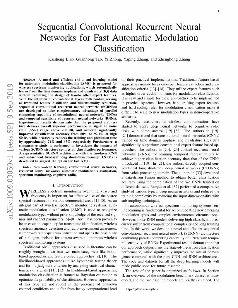
The classification accuracy of all the models are presentedin Fig. 2. It can be seen that the proposed SCRNN modeldelivers a significantly improved accuracy of 92.1% at highSNRs. The CNN and LSTM model as baselines are comparedto the proposed SCRNN model. It shows that the SCRNNmodel consistently achieves higher accuracy than the othertwo baselines in the SNR range from −10 dB to 18 dB, andsignificantly outperforms the CNN baseline model by 12%

Fig. 2. Classification accuracy comparison of the proposed SCRNN modelwith others on the benchmark dataset.

and the LSTM baseline model by 6% improvement at highSNRs. Additionally, it is observed that the proposed SCRNNmodel achieves exceeding performance than that of the CNNand LSTM baseline models in the SNR range from −10 dB to0 dB, where the two baseline models behave nearly the same.It implies that the convolutional layers of the SCRNNs servingas feature distillation boost the learning ability of the temporalfeatures under low SNR circumstances. The traditional supportvector machine (SVM) approach showing poor classificationperformance is also summarized in Fig. 2 for comparison. Allmodels are fed with the same training and test data of IQformat for this comparison except for the LSTM model withamplitude-phase format.

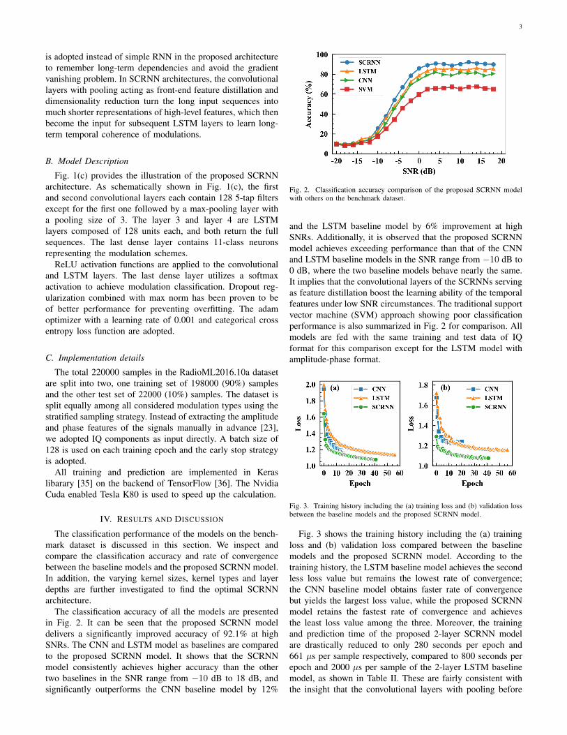
Fig. 3. Training history including the (a) training loss and (b) validation lossbetween the baseline models and the proposed SCRNN model.

Fig. 3 shows the training history including the (a) trainingloss and (b) validation loss compared between the baselinemodels and the proposed SCRNN model. According to thetraining history, the LSTM baseline model achieves the secondless loss value but remains the lowest rate of convergence;the CNN baseline model obtains faster rate of convergencebut yields the largest loss value, while the proposed SCRNNmodel retains the fastest rate of convergence and achievesthe least loss value among the three. Moreover, the trainingand prediction time of the proposed 2-layer SCRNN modelare drastically reduced to only 280 seconds per epoch and661 µs per sample respectively, compared to 800 seconds perepoch and 2000 µs per sample of the 2-layer LSTM baselinemodel, as shown in Table II. These are fairly consistent withthe insight that the convolutional layers with pooling before

4

TABLE IITRAINING AND PREDICTION TIME COMPARISON BETWEEN THE TWO

BASELINE MODELS AND THE THREE SCRNN MODELS.

Models CNN LSTM1-LayerSCRNN

2-LayerSCRNN

3-LayerSCRNN

Training Timeper Epoch (s)

30 800 800 280 90

Training Epochs 20 56 57 41 57Total TrainingTime (s)

600 44800 45600 11480 5130

Prediction Time(µs/sample)

1000 2000 641 661 751

RNN serve as feature distillation and dimensionality reduction,analogous to front-end matched filters, synchronizer and sam-pler for temporal features in typical wireless systems. To gainintuition on what convolution layers are learning in SCRNNarchitectures, the response patterns of the 128 filters learned bythe first convolutional layer are illustrated in Fig. 4, showingthat some filters encode expert-like patterns (i.e. BPSK-likepattern in row 1 column 6) and others even encode morecomplicated patterns. It further confirms that the convolutionallayers of the SCRNNs act as front-end feature distillation withcoherent features refined and redundant features filtered out,enabling the improved rate of convergence.

Fig. 4. Response patterns of the 128 filters learned by the first convolutionallayer of the SCRNN.

To gain more insight into the SCRNN architecture, we fur-ther investigate the effects of various SCRNN structure settingsvarying CNN kernel sizes, CNN layer depths, CNN kernelnumbers, RNN types and RNN layer depths on classificationperformance.

As shown in Fig. 5(a), varying the CNN kernel sizes of theSCRNNs has minimal impact on classification performance.The architecture with kernel size of 5 produces slightly betterclassification accuracy than others in SNR range from 0 dBto 18 dB, while the architecture with kernel size of 3 leads tomarginally higher classification accuracy in SNR range from-10 dB to -6 dB. The kernel size of 5 is used for the remainingexperiments.

Fig. 5(b) proves that the reduction of the input dimension-ality for subsequent LSTM layers in the SCRNN architectures

Fig. 5. Classification performance of different SCRNN structure configura-tions for varying (a) CNN kernel sizes, (b) CNN layer depths, (c) CNN kernelnumbers, (d) RNN types and layer depths.

shows very limited effects on classification performance. Asshown in Fig. 1 and Table II, the 2-layer SCRNN model re-duces the dimensionality by a factor of 3. This leads the train-ing and prediction time reduced by 74% and 67% respectively,while the performance remains nearly the same. However,the performance of the LSTM baseline model starts to decaysignificantly when reducing the input dimensionality [32]. Itis implied that the SCRNN architecture is much more robustto dimensionality reduction and training and prediction timeminimization. Thus, it makes possible for deploying onlinelearning model on autonomous wireless spectrum monitoringsystems.

Fig. 5(c) provides that the 64-kernel and 128-kernel struc-tures deliver the very similar performance, while the per-formance of 256-kernel structure starts to drop due to theoverfitting. Fig. 5(d) shows the different settings of RNNtypes and layer depths in the SCRNN architectures. It can beobserved that the performance of the LSTM type is apparentlysuperior to that of the gated recurrent unit (GRU) and simpleRNN type. Experimental results of varying LSTM layer depthssuggest that the 2-layer LSTM of the SCRNN achieves thebest classification accuracy. Therefore, the optimal SCRNNarchitecture with the 2-layer CNN and subsequent 2-layerLSTM is recommended for online learning.

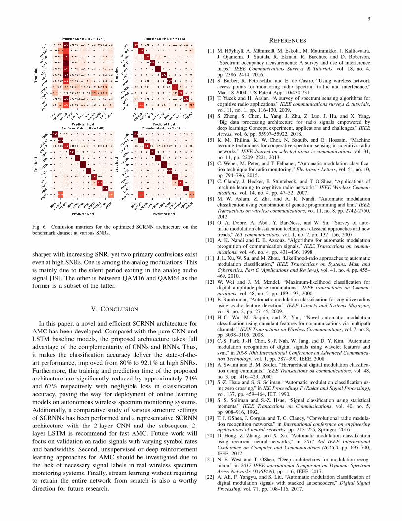
To evaluate how classification performance varies withSNRs, confusion matrices of the optimal SCRNN modelat various SNRs are investigated. For a confusion matrix,each column represents the predicted modulation type andeach row represents the real modulation type. The numericalvalue on each grid denotes the prediction probability of thecorresponding modulation type.

As illustrated in Fig. 6, the diagonals become gradually

5

Fig. 6. Confusion matrices for the optimized SCRNN architecture on thebenchmark dataset at various SNRs.

sharper with increasing SNR, yet two primary confusions existeven at high SNRs. One is among the analog modulations. Thisis mainly due to the silent period exiting in the analog audiosignal [19]. The other is between QAM16 and QAM64 as theformer is a subset of the latter.

V. CONCLUSION

In this paper, a novel and efficient SCRNN architecture forAMC has been developed. Compared with the pure CNN andLSTM baseline models, the proposed architecture takes fulladvantage of the complementarity of CNNs and RNNs. Thus,it makes the classification accuracy deliver the state-of-the-art performance, improved from 80% to 92.1% at high SNRs.Furthermore, the training and prediction time of the proposedarchitecture are significantly reduced by approximately 74%and 67% respectively with negligible loss in classificationaccuracy, paving the way for deployment of online learningmodels on autonomous wireless spectrum monitoring systems.Additionally, a comparative study of various structure settingsof SCRNNs has been performed and a representative SCRNNarchitecture with the 2-layer CNN and the subsequent 2-layer LSTM is recommend for fast AMC. Future work willfocus on validation on radio signals with varying symbol ratesand bandwidths. Second, unsupervised or deep reinforcementlearning approaches for AMC should be investigated due tothe lack of necessary signal labels in real wireless spectrummonitoring systems. Finally, stream learning without requiringto retrain the entire network from scratch is also a worthydirection for future research.

REFERENCES

[1] M. Hoyhtya, A. Mammela, M. Eskola, M. Matinmikko, J. Kalliovaara,J. Ojaniemi, J. Suutala, R. Ekman, R. Bacchus, and D. Roberson,“Spectrum occupancy measurements: A survey and use of interferencemaps,” IEEE Communications Surveys & Tutorials, vol. 18, no. 4,pp. 2386–2414, 2016.

[2] S. Barber, R. Petruschka, and E. de Castro, “Using wireless networkaccess points for monitoring radio spectrum traffic and interference,”Mar. 18 2004. US Patent App. 10/430,731.

[3] T. Yucek and H. Arslan, “A survey of spectrum sensing algorithms forcognitive radio applications,” IEEE communications surveys & tutorials,vol. 11, no. 1, pp. 116–130, 2009.

[4] S. Zheng, S. Chen, L. Yang, J. Zhu, Z. Luo, J. Hu, and X. Yang,“Big data processing architecture for radio signals empowered bydeep learning: Concept, experiment, applications and challenges,” IEEEAccess, vol. 6, pp. 55907–55922, 2018.

[5] K. M. Thilina, K. W. Choi, N. Saquib, and E. Hossain, “Machinelearning techniques for cooperative spectrum sensing in cognitive radionetworks,” IEEE Journal on selected areas in communications, vol. 31,no. 11, pp. 2209–2221, 2013.

[6] C. Weber, M. Peter, and T. Felhauer, “Automatic modulation classifica-tion technique for radio monitoring,” Electronics Letters, vol. 51, no. 10,pp. 794–796, 2015.

[7] C. Clancy, J. Hecker, E. Stuntebeck, and T. O’Shea, “Applications ofmachine learning to cognitive radio networks,” IEEE Wireless Commu-nications, vol. 14, no. 4, pp. 47–52, 2007.

[8] M. W. Aslam, Z. Zhu, and A. K. Nandi, “Automatic modulationclassification using combination of genetic programming and knn,” IEEETransactions on wireless communications, vol. 11, no. 8, pp. 2742–2750,2012.

[9] O. A. Dobre, A. Abdi, Y. Bar-Ness, and W. Su, “Survey of auto-matic modulation classification techniques: classical approaches and newtrends,” IET communications, vol. 1, no. 2, pp. 137–156, 2007.

[10] A. K. Nandi and E. E. Azzouz, “Algorithms for automatic modulationrecognition of communication signals,” IEEE Transactions on commu-nications, vol. 46, no. 4, pp. 431–436, 1998.

[11] J. L. Xu, W. Su, and M. Zhou, “Likelihood-ratio approaches to automaticmodulation classification,” IEEE Transactions on Systems, Man, andCybernetics, Part C (Applications and Reviews), vol. 41, no. 4, pp. 455–469, 2010.

[12] W. Wei and J. M. Mendel, “Maximum-likelihood classification fordigital amplitude-phase modulations,” IEEE transactions on Commu-nications, vol. 48, no. 2, pp. 189–193, 2000.

[13] B. Ramkumar, “Automatic modulation classification for cognitive radiosusing cyclic feature detection,” IEEE Circuits and Systems Magazine,vol. 9, no. 2, pp. 27–45, 2009.

[14] H.-C. Wu, M. Saquib, and Z. Yun, “Novel automatic modulationclassification using cumulant features for communications via multipathchannels,” IEEE Transactions on Wireless Communications, vol. 7, no. 8,pp. 3098–3105, 2008.

[15] C.-S. Park, J.-H. Choi, S.-P. Nah, W. Jang, and D. Y. Kim, “Automaticmodulation recognition of digital signals using wavelet features andsvm,” in 2008 10th International Conference on Advanced Communica-tion Technology, vol. 1, pp. 387–390, IEEE, 2008.

[16] A. Swami and B. M. Sadler, “Hierarchical digital modulation classifica-tion using cumulants,” IEEE Transactions on communications, vol. 48,no. 3, pp. 416–429, 2000.

[17] S.-Z. Hsue and S. S. Soliman, “Automatic modulation classification us-ing zero crossing,” in IEE Proceedings F (Radar and Signal Processing),vol. 137, pp. 459–464, IET, 1990.

[18] S. S. Soliman and S.-Z. Hsue, “Signal classification using statisticalmoments,” IEEE Transactions on Communications, vol. 40, no. 5,pp. 908–916, 1992.

[19] T. J. OShea, J. Corgan, and T. C. Clancy, “Convolutional radio modula-tion recognition networks,” in International conference on engineeringapplications of neural networks, pp. 213–226, Springer, 2016.

[20] D. Hong, Z. Zhang, and X. Xu, “Automatic modulation classificationusing recurrent neural networks,” in 2017 3rd IEEE InternationalConference on Computer and Communications (ICCC), pp. 695–700,IEEE, 2017.

[21] N. E. West and T. OShea, “Deep architectures for modulation recog-nition,” in 2017 IEEE International Symposium on Dynamic SpectrumAcess Networks (DySPAN), pp. 1–6, IEEE, 2017.

[22] A. Ali, F. Yangyu, and S. Liu, “Automatic modulation classification ofdigital modulation signals with stacked autoencoders,” Digital SignalProcessing, vol. 71, pp. 108–116, 2017.

6

[23] S. Rajendran, W. Meert, D. Giusiniano, V. Lenders, and S. Pollin, “Deeplearning models for wireless signal classification with distributed low-cost spectrum sensors,” IEEE Transactions on Cognitive Communica-tions and Networking, vol. 4, no. 3, pp. 433–445, 2018.

[24] T. J. OShea, T. Roy, and T. C. Clancy, “Over-the-air deep learning basedradio signal classification,” IEEE Journal of Selected Topics in SignalProcessing, vol. 12, no. 1, pp. 168–179, 2018.

[25] M. Sadeghi and E. G. Larsson, “Adversarial attacks on deep-learningbased radio signal classification,” IEEE Wireless Communications Let-ters, vol. 8, no. 1, pp. 213–216, 2018.

[26] D. Zhang, W. Ding, B. Zhang, C. Xie, H. Li, C. Liu, and J. Han, “Au-tomatic modulation classification based on deep learning for unmannedaerial vehicles,” Sensors, vol. 18, no. 3, p. 924, 2018.

[27] C.-F. Teng, C.-C. Liao, C.-H. Chen, and A.-Y. A. Wu, “Polar featurebased deep architectures for automatic modulation classification consid-ering channel fading,” in 2018 IEEE Global Conference on Signal andInformation Processing (GlobalSIP), pp. 554–558, IEEE, 2018.

[28] J. Sun, G. Wang, Z. Lin, S. G. Razul, and X. Lai, “Automatic modulationclassification of cochannel signals using deep learning,” in 2018 IEEE23rd International Conference on Digital Signal Processing (DSP),pp. 1–5, IEEE, 2018.

[29] M. Kulin, T. Kazaz, I. Moerman, and E. De Poorter, “End-to-endlearning from spectrum data: A deep learning approach for wirelesssignal identification in spectrum monitoring applications,” IEEE Access,vol. 6, pp. 18484–18501, 2018.

[30] B. Tang, Y. Tu, Z. Zhang, and Y. Lin, “Digital signal modulationclassification with data augmentation using generative adversarial netsin cognitive radio networks,” IEEE Access, vol. 6, pp. 15713–15722,2018.

[31] S. Zheng, P. Qi, S. Chen, and X. Yang, “Fusion methods for cnn-basedautomatic modulation classification,” IEEE Access, 2019.

[32] S. Ramjee, S. Ju, D. Yang, X. Liu, A. E. Gamal, and Y. C. Eldar, “Fastdeep learning for automatic modulation classification,” arXiv preprintarXiv:1901.05850, 2019.

[33] Y. Wang, M. Liu, J. Yang, and G. Gui, “Data-driven deep learning forautomatic modulation recognition in cognitive radios,” IEEE Transac-tions on Vehicular Technology, vol. 68, no. 4, pp. 4074–4077, 2019.

[34] T. J. O’shea and N. West, “Radio machine learning dataset generationwith gnu radio,” in Proceedings of the GNU Radio Conference, vol. 1,2016.

[35] F. Chollet et al., “Keras: The python deep learning library,” AstrophysicsSource Code Library, 2018.

[36] M. Abadi, P. Barham, J. Chen, Z. Chen, A. Davis, J. Dean, M. Devin,S. Ghemawat, G. Irving, M. Isard, et al., “Tensorflow: A systemfor large-scale machine learning,” in 12th {USENIX} Symposium onOperating Systems Design and Implementation ({OSDI} 16), pp. 265–283, 2016.