sequential optimal designs for on-line …rutcor.rutgers.edu/pub/rrr/reports99/02.pdfa department of...
TRANSCRIPT

R U T C O R
R E S E A R C H
R E P O R T
������
����� � � ��
������ � �����
����� � ������
��� ��������� ����
���������� !� "��
�##$�%#��&
����� ' (&)%��$%&#��
����*' (&)%��$%$�()
+����' ,����-����-��
����'..����-����-��./
SEQUENTIAL OPTIMALDESIGNS FOR ON-LINE ITEM
CALIBRATION
Douglas. H. Jonesa Mikhail Nediakb
Xiang-Bo Wangc
RRR 2-99, February, 1999
a Department of Management Science and Information Systems, Rutgers, theState University of New Jersey, 180 University Av./Ackerson Hall, Newark,NJ 07102-1803, USA, [email protected] RUTCOR, Rutgers, The State University of New Jersey, 640 BartholomewRoad, Piscataway, NJ 08854-8003, USA, [email protected] Operations and Test Development Research, Law School AdmissionsCouncil, Box 40, 661 Penn Street, Newtown, PA, 18940-0040, USA.
RUTCOR RESEARCH REPORTRRR 2-99, FEBRUARY, 1999
SEQUENTIAL OPTIMAL DESIGNS FORON-LINE ITEM CALIBRATION
Douglas H. Jones Mikhail S. Nediak Xiang-Bo Wang
Abstract. In an on-line adaptive test, data for calibrating new items are collected from examinees whilethey take an operational test. In this paper, we will assume a situation where a calibration session mustcollect data about several experimental items simultaneously. While past research has focused onestimation of one or more two-parameter logistic items, this research focuses on estimating several three-parameter logistic items simultaneously. We consider this problem in terms of constrained optimizationover probability distributions. The probability distributions are over a two-by-two contingency table, andthe marginal distributions form the constraints. We formulate these constraints for network-flowconstraint, and investigate a conjugate-gradient-search algorithm to optimize the determinant of Fisher’sinformation matrix.Keywords and phrases: Optimal design, item spiraling, item response theory, psychological testing,computerized adaptive tasting, network flow mathematical programming, nonlinear response function.
Acknowledgements: This study received funding from the Law School Admission Council (LSAC). Theopinions and conclusions contained in this report are those of the author and do not necessarily reflect theposition or policy of LSAC. The work of D.H. Jones was partially supported by the Cognitive ScienceProgram of the Office of the Chief of Naval Research under Contact N00012-87-0696.

1 IntroductionIn an on-line adaptive test, data for calibrating new items are collected from examinees while they
take an operational test. In this paper, we will assume a situation where a calibration session must
collect data about several experimental items simultaneously. Other researchers have recognized
the advantages of using optimal sampling designs to calibrate items (van der Linden, 1988)
(Berger, 1991, 1992, 1994) (Berger and van der Linden, 1991) and (Jones and Jin, 1994). While
past research has focused on estimation of one or more two-parameter logistic items, this research
focuses on estimating several three-parameter logistic items simultaneously. This problem is
considered as an unconstrained nonlinear mathematical programming model in Berger (1994).
We consider this problem in terms of constrained optimization over probability distributions. The
probability distributions are over a two-by-two contingency table, and the marginal distributions
form the constraints. We formulate these constraints for network-flow constraints (Ahuja,
Magnanti and Orlin, 1993), and investigate a conjugate-gradient-search algorithm to optimize the
determinant of Fisher’s information matrix (Murtaugh and Saunders, 1978).
In next section 2, we introduce D-Optimality. Section 3 states the mathematical program,
constraints, and solution technique, namely projected conjugate-gradient. Section 4 described the
sequential estimation schemes that employ D-optimal designs. Section 5 presents simulation
results using actual LSAT item data, followed by the conclusion in Section 6. The gradient of the
Fisher information matrix for the 3PL item is derived in Appendix 8.1. The projection on the null
space of the constraint matrix is derived in Appendix 8.2.
2 D-optimal design criterionLet ui denote a response to a single item from individual i with ability level θi, possibly
multivariate. Let βT = (β0,β1…βp) be a vector of unknown parameters associated with the item.
Assume that all responses are scored either correct; ui = 1, or incorrect, ui = 0. An item response

function, P(θi, β), is a function of θi, and describes the probability of correct response of an
individual with ability level θi. The mean and variance of the parametric family are
E u Pi i| ;β β� � � �= θ (1)
σ θ θ θ2 1i i i iVar u P P; | ; ;β β β β� � � � � � � �= = − . (2)
We shall focus on the family of three-parameter logistic (3PL) response functions:
P Ri iθ β β θ; ;ββ ββ� � � � � �= + −2 21 , (3)
where
Re
eiθβ β θ
β β θ;β� � =+
+
+
0 1
0 11. (4)
Denote three IRT characteristics of a three-parameter item to be: the discrimination power, a =
1.7*β1; the difficulty, b = -β0/β1, guessing, c = β2. Note the family of two-parameter logistic
(2PL)-response function is expression (3) β2 = 0.
The expected information from ability θ is defined as Fisher’s information matrix. The 3PL-
information matrix is
m ββ
β β
β β β
β β ββ β
;;
; ;
; ; ;
; ; ;
; ;
θθ
θ θ
β θ β θ θ β θ
β θ θ β θ θ β θ θβ θ β θ θ
� �� �
� � � �
� � � � � � � � � � � �� � � � � � � � � � � �� � � � � � � �
=−
−
− − −
− − −− −
�
�
���
�
1
1
1 1 1
1 1 1
1 1 1
2 2
2 2
2
2 2
2
2
2 2
2
2 2 22
2 2
R
P P
R R R
R R R
R R
. (5)
We are interested in assigning test-takers to items so that the greatest about of information
about the item parameters can be obtained. Assume point estimates of test-takers’ ability are
available, denoted by Θ = {θi: i = 1,…,n}. Assume initial point estimates of item vectors are
available, denoted by B = {βj: j = 1,…,m}. Denote the information obtained from pairing ability
θi with item vector βj by

m mi jj i
, ;� � � �= ββ θ . (6)
Introduce xij equal to the number of observations taken for item j from ability i. Then by the
additive property of Fisher’s information, the information matrix of item j is
M M x mj jj ij
i j
i
n
x� � � � � �� �≡ ==∑β ; , ,Θ
1
(7)
where x = (x11,…, x1n; x21,…, x2n;…; xm1,…, xmn). If observations for different items are taken
independently, the information matrix for all items taken together is
M B x M; ,� � �� �= diag j . (8)
We call a design X exact if xij is an integer for all i and j; otherwise, we call it approximate. An
optimal design will typically be an approximate design.
The design criterion we wish to consider is
log det ; , log det ; ,M B x M xΘ Θ� � � �� �==
∑ jj
j
n
β1
. (9)
For a single item problem, this criterion is the classical D-optimal criterion. For which there exist
practical methods for deriving D-optimal designs (Donev and Atkinson, 1988), (Haines, 1987),
(Mitchell, 1974), (Welch, 1982). See (Silvey, 1980) for other criteria. Approximate D-optimal
designs are derived in (Ford, 1976) for a single item using the continuous design space [-1, 1],
which are discrete, equal probability, two-point distributions with support points depending on
the values of the item parameters. A simplification of the support points is approximately
±min{1, 1.5434(Dβ1)-1} (Jones and Jin, 1994). In the present investigation, the design space is
the set of all pairings between test-takers and items, and the design specifies which parings
between test-takers and items will be observed. Jones, Chiang, and Jin (1997) derived solutions
for this problem when the response functions were limited to the 2PL family.

3 Mathematical Program and Solution for optimal designsConsider the problem of selecting xij, the number of observations taken for item j from ability i, to
maximize information. A mathematical programming model for finding an optimal design with
marginal constraints on x = {xij: i = 1…n; j = 1…m} is the following:
Maximizelog det ; ,M B x� �
such that
x s i nijj
m
=∑ = =
1
1; ,..., (10)
x d j miji
n
=∑ = =
1
1; , ..., (11)
x i n j mij ≥ = =0 1 1; ,..., ; ,..., (12)
where md = ns.
Constraints (10) stipulate that there is a supply of s test-takers with ability θi, and all these test-
testers must receive an item. Constraints (11) stipulate that each item j demands d test-takers.
Constraints (12) insure that the solution is logically consistent. The requirement md = ns ensures
that the total item demand is equal to the total supply of test-takers.
The constraint matrix corresponding to constraints (10) and (11) is derived as follows. Denote
Im and I n as m by m and n by n identity matrices, respectively. In addition, denote em and en as m
and n column vectors of all 1’s. Define the following constraint matrix:
A
I I I
e
e
e
=
�
�
�����
�
n n n
nT
nT
nT
�
�
�
� � � �
�
0 0
0 0
0 0
(13)
Define,

be
e=���
�
s
dn
m
. (14)
Then the
Ax = b (15)
is a restatement of the constraints (10) and (11). A point x 0≥ is feasible if it satisfies (15). If
x 0> is feasible and α is an arbitrary sufficiently small scalar, then, a point x +αr is feasible if
and only if Ar = 0; that is, if r is in the null space of A.
The objective function for this problem is known to be concave in x (Federov, 1972). We use
the conjugate-gradient methods for linearly constrained problems and logarithmic penalty
functions for the non-negativity constraints (12) to get approximate designs (for an overview of
optimality procedures, see Gill, Murray and Wright, 1981). Thus, our objective function becomes:
F F xiji j
x x M B x� � � � � �≡ = + ∑µ µlog det ; , log,
Θ (16)
where µ is a penalty parameter; this parameter is sequentially reduced to a sufficiently small
value.
The unconstrained conjugate-gradient method is described as follows. Assume that xk is an
approximation to the maximum of F. Given a direction of search pk, let
α αα
∗ = +arg maxF k kx p� � . (17)
The next approximation to the maximum of F is
x x pk k k+∗= +1 α . (18)
Denote the gradient of F at xk as g(xk) (see Appendix 8.1 for its derivation). The direction of
search, obtained from the method of conjugate-gradient, is defined as:

p g x pg x g x g x
g xk k k
k
T
k k
k
= +−
−−
−
� �� � � � � �
� �1
1
1
2 . (19)
Where pk-1 and xk-1 denote the previous search direction and approximation, respectively. The
conjugate-gradient must be restarted in the direction of steepest ascent every nm steps.
The constrained conjugate-gradient method is an extension of the foregoing method. The
linearly constrained problem uses the projection of the direction (19) on the null space of the
constraint matrix (13). Denote p as an nm dimensional direction vector. In the appendix we
derive the following simple expression for the ij th component of the projection r of p on {x: Ax =
0}:
r pm
pn
pmn
pij ij ill
m
kjk
n
klk l
= − − += =
∑ ∑ ∑1 1 1
1 1 ,
. (20)
This result is not very surprising in light of the theory of analysis of variance in statistics using pij
for data, as these elements are known as interactions in the two-way model with main effects for
item and ability. They are the least-squares residuals from the fitted values in the main effects
model, and thus must lie in the null space of the constraints (10) and (11). Note that searching
from a feasible point in the direction of r ensures feasibility of the solution.
4 Sequential Estimation of Item ParametersIn item response theory, optimal designs depend on knowing the item parameters. For obtaining
designs for the next stage of observations, a sequential estimation scheme supplies item
parameters that should converge to the true parameters. By continually improving the item
parameters, the solutions of mathematical program yield better designs for obtaining data that are
more efficient.
We have had experience with maximum likelihood and Baysian methods. Application of both
maximum likelihood and Baysian methods are straightforward. The choice between these two

methods may be decided from numerical considerations. Maximum likelihood may be unstable
for the beginning of the sequential procedure, as the likelihood is nearly flat. Baysian methods
enjoy stability, but the choice of a prior may be a difficult. In the following section, we study the
performance of optimal design methods using Baysian estimators incorporating uninformative
and informative priors.
5 Computational ResultsWe present some results using actual data from paper-and-pencil administration of the LSAT
using the 3PL model. The data consist of the responses to 101 items from 1600 test-takers. We
use this data to simulate an on-line item calibration. Five items will be calibrated. Batches of 40
test-takers are randomly chosen. Each item receives five test-takers. No test-taker receives more
than one item. Initial estimates of � are fed to the mathematical program and a design is derived.
The design specifies what records of test-takers are used to estimate the parameters of each item.
This process continues for 40 batches of test-takers. Then another set of items is chosen for the
next calibration round, until all items have been calibrated. The following is a summary of the
simulation components:
5.1 SIMULATION STRATEGY
Items are calibrated in sets of 5 items. Each run of 40 test-takers yields 8 new observation for
each item. After each run, estimates of item parameters are updated. After the initial run, each run
is designed to obtain D-optimal Fisher information for item parameters. A total of 40 runs were
performed, resulting in 320 observations per item
5.2 ESTIMATION STRATEGIES
Strategy R: Uniform priors; 40 runs random BB design

Strategy A: Uniform priors; one run random BB design; 39 runs optimal design
Strategy D: Priors set equal to posteriors from 40 runs BB design; 40 runs optimal design
Random BB denotes a balanced block design, where the test-takers are blocked into eight
groups according to ability and then assigned randomly to items. An optimal design is derived
using Bayes EAP estimators based on the accumulated data and designated prior.
5.3 NOTATION
E denotes the estimation error of �0, �1, �2. The numbers 0, 1, 2 identify the parameters �0, �1,
�2. R, A, D identifies the estimation strategy, e.g. EA0, EA1, EA2 are estimation errors with
strategy A
In addition, we use a measure of overall fit of the item response function. The Hellinger
distance between two discrete probability distributions f1(x) and f2(x) is
H f x f xi ii
= −=
∞
∑ 11 2
21 2 2
1
/ /( ) ( )� � .In our case, if we have two parameter estimates β and β’ , the Hellinger distance between
corresponding IRF’s at a particular ability level θ can be computed as (after a simple
transformation):
H P Pθ θ θ( , ) ( , ) ( , )β β β β′ = − ′2 1� �.The weighted integral Hellinger distance between IRF’s is obtained by integrating out θ with
respect to some suitable weight function w(θ ):
H P P w d( , ) ( , ) ( , ) ( )β β β β′ = − ′−∞
+∞
�2 1 θ θ θ θ� �
In this particular case we have chosen w(θ ) to be proportional to the probability density function
of N(1,1) distribution since deviations over this distribution of ability would be most important.

These will be denoted as H with designation for estimation strategy; e.g., HD is the Hellinger
distance associated with strategy D.
5.4 RESULTS
The true parameters are derived from estimation with all 1600 records for each item. The
sequential estimates are based on 320 observations each, derived as explained above. In general,
320 random observations would not yield very satisfactory parameter estimates. However, the use
of sequentially derived optimal designs increases the effectiveness of the relatively small number
of observations, as can be seen with the percentiles of estimation errors displayed in Table 1.
Table 2 displays the percentiles of Hellinger distance over the three estimation strategies.
Strategy D appears to fit better than either A or D.
Table 3 displays estimation errors and Hellinger distances of the two extreme items of each
estimation strategies. Figure 1 displays the true and estimated item response functions of the these
items.
6 ConclusionD-optimal designs improve item calibration over the random design considered in this paper. The
estimation is better with informative priors. Linear hierarchical priors may be employed to obtain
priors that are more informative. These may be obtained from past calibrations and, possibly,
information about the item. Other design criteria could be employed, e.g. Buyske (1998a,b).
Clearly, some items were calibrated more effectively than others. In actual implementation of
on-line item calibration, the more easily calibrated items could be removed from sampling earlier.
Computational times for deriving optimal designs were well within bounds for implementation in
an actual setting.

ReferencesAhuja, R. K., Magnanti, T. L., & Orlin, J. B. (1993). Network flows: Theory, algorithms, and
applications. Englewood Cliffs, NJ: Prentice-Hall.
Berger, M. P. F. (1991). On the efficiency of IRT models when applied to different sampling
designs. Applied Psychological Measurement, 15, 283-306.
Berger, M. P. F. (1992). Sequential sampling designs for the two-parameter item response
theory model. Psychometrika, 57, 521-538.
Berger, M. P. F. (1994). D-Optimal sequential designs for item response throe models. Journal
of Educational Statistics, 19, 43-56.
Berger, M. P. F., & van der Linden, W. J. (1991). Optimality of sampling designs in item
response theory models. In M. Wilson (Ed.), Objective measurement: Theory into practice.
Norwood, NJ: Ablex Publishing.
Buyske, S. G. (1998a). Item calibration in computerized adaptive testing using minimal
information loss. Preprint.
Buyske, S. G. (1998b). Optimal designs for item calibration in computerized adaptive testing.
Unpublished doctoral dissertation, Rutgers University of New Jersey.
Donev, A. N. & Atkinson, A. C. (1988). An adjustment algorithm for the construction of exact
D-optimum experimental designs. Technometrics, 30, 429-433.
Federov, V. V. (1972). Theory of optimal experiments. New York: Academic Press.
Ford, I. (1976). Optimal static and sequential design: A critical review. Unpublished doctoral
dissertation, University of Glasgow.
Gill, P. E., Murray, W., & Wright, M. H. (1981). Practical optimization. London: Academic
Press.

Haines, L. M. (1987). The application of the annealing algorithm to the construction of exact
optimal designs for linear-regression models. Technometrics, 29, 439-447.
Jones, D. H., & Jin, Z. (1994). Optimal sequential designs for on-line item estimation.
Psychometrika, 59, 59-75.
Jones, D. H., Chiang, J, & Jin, Z. (1997). Optimal designs for simultaneous item estimation.
Nonlinear Analysis, Theory, Methods & Applications, 30, 4051-4058.
Lord, F. M. (1980). Applications of item response theory to practical testing problems. Hillside,
NJ: Erlbaum.
Mitchell, T. J. (1974). An algorithm for the construction of D-optimal experimental designs.
Technometrics, 16, 203-210.
Murtaugh, B., & Saunders, M. (1978). Large scale linearly constrained optimization. Math.
Program., 14, 42-72.
Nemhauser, G., & Wolsey, L. (1988). Integer and combinatorial optimization. New York:
Wiley.
Prakasa Rao, B. L. S. (1987). Asymptotic theory of statistical inference. New York: Wiley.
Silvey, S. D. (1980). Optimal design. New York: Chapman and Hall.
Van der Linden, W. J. (1988). Optimizing incomplete sampling designs for item response model
parameters (Research Report No. 88-5). Enschede, The Netherlands: University of
Twente.
Welch, W. J. (1982). Branch-and-bound search for experimental designs based on D optimality
and other criteria. Technometrics, 24, 41-48.
Appendix
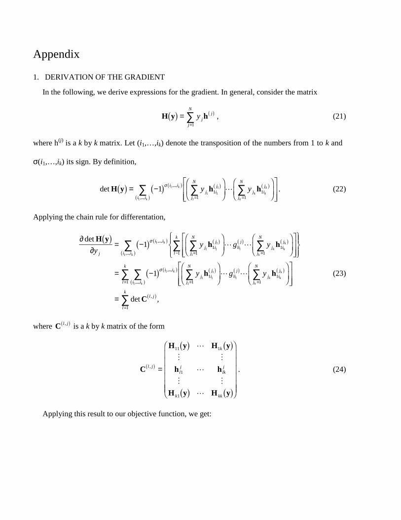
1. DERIVATION OF THE GRADIENT
In the following, we derive expressions for the gradient. In general, consider the matrix
H y h� � � �==
∑ y jj
j
N
1
, (21)
where h(j) is a k by k matrix. Let (i1,…,ik) denote the transposition of the numbers from 1 to k and
σ(i1,…,ik) its sign. By definition,
det,...,
,...,
H y h h� � � � � � � � � �
� �= −
���
����
�
�
���
�
���= =
∑ ∑∑ 1 1
1 1
1
11
11
11
σ i i
j ij
j
N
j ij
j
N
i i
k
k k
k
kk
y y� . (22)
Applying the chain rule for differentation,
∂∂
= −���
�
���
�
�
���
�
���
�����
�����
= −���
�
�= =−
= =
∑ ∑∑∑
∑ ∑
det ,...,
,...,
,...,
H yh h
h h
� � � �
� �
� � � � � � � �
� �
� � � � � � � �
yy g y
y g y
j
i i
j ij
j
N
lij
j ij
j
N
l
k
i i
i i
j ij
j
N
lij
j ij
j
N
k
l k k
k
kk
k
l k k
k
k
1
1
1
1 1
1
11
1
1 1
1
1
11
111
11
11
σ
σ
� �
� ���
�
�
���
�
���
=
∑∑
∑
=
=
i il
k
l j
l
k
k11
1
,...,
,det ,
� �
� �C
(23)
where C l j,� � is a k by k matrix of the form
C
H y H y
h h
H y H y
l j
k
lj
lkj
k kk
,� �
� � � �
� � � �
=
�
�
������
�
11 1
1
1
�
� �
�
� �
�
. (24)
Applying this result to our objective function, we get:

∂∂
=
�
�
���
�
+
�
�
���
�
+
+
log det ; ,
det
det det
det
, , ,
, , ,
M B X
M
m m m
M M M
M M M
M M M
m m m
M M M
M M M
M M M
� �� �
� � � � � �
� � � � � �
� � � � � �
� � � � � �
� � � � � �
� � � � � �
� � � � � �
� � � � �
xijj
i j i j i j
j j j
j j j
j j j
i j i j i j
j j j
j j j
j j j
1
11 12 13
21 22 23
31 32 33
11 12 13
21 22 23
31 32 33
11 12 13
21 22 123�
� � � � � �m m m31 32 33i j i j i j, , ,
�
�
���
�
�
�
����
�
����
�
�
����
�
����
.
(25)
2. PROJECTIONS ON THE NULL SPACE OF THE CONSTRAINT MATRIX
Denote p as an nm dimensional direction vector. Denote Im and I n as m by m and n by n
identity matrices, respectively. In addition, denote em and en as m and n column vectors of all 1’s.
Define the following constraint matrix:
A
I I I
e
e
e
=
�
�
�����
�
n n n
nT
nT
nT
�
�
�
� � � �
�
0 0
0 0
0 0
(26)
The projection r of p on {y: Ay = 0}, the null space of A, is given by
r p A y= − T , (27)
where y is a solution to
AA y ApT� � = . (28)
Introduce the following notation:
yy
yAp
p
py p R y p R=
���� =
���� ∈ ∈1
2
1
21 1 2 2;
~
~ ; ,~ ; ,~n m . (29)
We have the following simplifications:
~ ,..., ;~ ,...,p p1 1 2 1= =• • • •p p p pn
T
m
T� � � � , (30)

where
p p p pi ijj
m
j iji
n
•=
•=
= =∑ ∑1 1
; , (31)
and
AAI E
E IT n
T
m
m
n=���
�
, (32)
where E is an m by n matrix of all ones. Consequently, equation (28) can be written as:
m
n
n mT
m nT
y e e y p
e e y y p
1 2 1
1 2 2
+ =
+ =
� �� �
~
~(33)
implying:
e y e y
y p e e y
y p e e y
nT
mT ij
i j
n mT
m nT
n m
p
nm
m
n
1 2
1 1 2
2 2 1
1
1
+ =
= −
= −
∑,
~
~
� �
� �
(34)
Thus
A y Ap
pA
ee y
ee y
Ap
pe
e y e y
T T Tn
mT
mnT
Tn m
mT
nT
m
n
m
n
m
nm n
=
�
�
���
�
−
���
�
���
�
�
�
����
�
=
=
�
�
���
�
− +���
�+
1
1
1
1
1
2
2
1
1
2
2 1
~
~
~
~
(35)
Denote z = ATy, then by (35),
zm
pn
pnm
pij i j klk l
= + −• • ∑1 1 1
,
. (36)

Since r = p - z, we have
rij ij i j klk l
pm
pn
pnm
p= − − +• • ∑1 1 1
,
. (37)

TablesTable 1. Percentiles of estimation errors over three estimation strategies.
-.58 -.48 -.27 -.08 .12 .36 .46
-.79 -.67 -.39 -.08 .13 .30 .38
-.71 -.50 -.27 -.05 .12 .25 .37
-.25 -.19 -.09 .03 .18 .33 .45
-.25 -.22 -.11 .06 .22 .32 .44
-.25 -.17 -.08 .06 .22 .36 .45
-.07 -.05 -.01 .02 .08 .11 .16
-.05 -.04 -.01 .03 .07 .16 .19
-.07 -.04 -.02 .01 .07 .13 .15
ER0
EA0
ED0
ER1
EA1
ED1
ER2
EA2
ED2
EstimationErrors
5 10 25 50 75 90 95
Percentiles

Table 2.Percentiles of Hellinger distance over three estimation strategies.
Percentiles5 10 25 50 75 90 95
Hellinger HR 0.00+ 0.00+ 0.00+ 0.00+ 0.01 0.02 0.04HA 0.00+ 0.00+ 0.00+ 0.00+ 0.02 0.04 0.06HD 0.00+ 0.00+ 0.00+ 0.00+ 0.01 0.02 0.03

Table 3. Estimation errors and Hellinger distances of extreme items of each estimation strategy.
ITEM67 ITEM25 ITEM53 ITEM100 ITEM57
β0 -2.47 -0.32 0.17 -0.52 -0.12
ER0 0.99 -1.48 -0.29 -0.49 -0.57
EA0 0.28 -1.20 -0.92 -0.79 -0.41
ED0 0.02 -0.37 -0.20 -0.84 -1.13
β1 1.74 0.72 0.95 0.73 0.49
ER1 -0.57 0.23 0.41 0.19 0.10
EA1 -0.25 0.31 0.23 0.50 0.13
ED1 0.10 0.27 0.00 0.57 0.36
β2 0.24 0.11 0.10 0.18 0.20
ER2 -0.09 0.22 0.06 0.06 0.20
EA2 0.00 0.19 0.25 0.15 0.14
ED2 -0.01 0.13 0.07 0.17 0.26
HR 0.04 0.09 0.02 0.02 0.02
HA 0.00+ 0.08 0.08 0.07 0.02
HD 0.00+ 0.03 0.00+ 0.08 0.09

Figure 1. Comparison of true and estimated item response functions of extremeitems of each estimation strategies
THETA
3.002.502.001.501.00.50.00-.50-1.00-1.50-2.00-2.50-3.00
1.2
1.0
.8
.6
.4
.2
0.0
PR67
P67
THETA
3.002.502.001.501.00.50.00-.50-1.00-1.50-2.00-2.50-3.00
1.2
1.0
.8
.6
.4
.2
0.0
PR25
P25
THETA
3.002.502.001.501.00.50.00-.50-1.00-1.50-2.00-2.50-3.00
1.2
1.0
.8
.6
.4
.2
0.0
PA25
P25
THETA
3.002.502.001.501.00.50.00-.50-1.00-1.50-2.00-2.50-3.00
1.2
1.0
.8
.6
.4
.2
0.0
PA53
P53
THETA
3.002.502.001.501.00.50.00-.50-1.00-1.50-2.00-2.50-3.00
1.2
1.0
.8
.6
.4
.2
0.0
PD100
P100
THETA
3.002.502.001.501.00.50.00-.50-1.00-1.50-2.00-2.50-3.00
1.2
1.0
.8
.6
.4
.2
0.0
PD57
P57