Nuclear Physics B362 (1991) 5 1 5 - 5 6 2

North-Holland

COVARIANT DIFFERENTIAL EQUATIONS AND SINGULAR VECTORS IN VIRASORO REPRESENTATIONS

M. BAUER

Sercice de Physique Th6orique de Saclay *, F-91191 Gif-sur-Ycette cedex, France

Ph. Di F R A N C E S C O

Joseph Henry Laboratories, Princeton Unicersity, Princeton, NJ 08544, USA

C. ITZYKSON and J.-B. ZUBER**

Sercice de Physique Th&)rique de Saclay, F-91191 Gif-sur-Ycette cedex, France

Received 20 March 1991

(Accepted for publication 24 April 1991)

We give explicit expressions for the singular vectors in highest weight representations of the Virasoro algebra using a precise definition of fusion.

1. Introduction

The rich representation theory of the Virasoro algebra has produced a vast amount of applications in statistical physics, conformal field theory and string theory. It is largely based on the fundamental work of Kac [1], Feigin and Fuchs [2] and Belavin et al. [3]. The Kac determinant formula yields the complex pattern of inclusions of Verma modules, leads to the consideration of rational theories and produces character formulas and differential equations for field correlations. The methods of proofs though improved by a number of authors [4-7], did not yet give very explicit expressions for these embeddings dictated by the existence of singular vectors in Verma modules. It is the aim of this work to produce such expressions.

A first important step - perhaps not sufficiently noticed - was accomplished by Benoit and Saint-Aubin [8] who gave a sub-series of these vectors. These formulas can be recast in a transparent matrix form in complete parallel to the formalism

* Laboratoire de la Direction des Sciences de la Matibre du Commissariat ~ I'Energie Atomique. ** E-mail address: zuber~poseidon.cea.fr

0 5 5 0 - 3 2 1 3 / 9 1 / $ 0 3 . 5 0 © 1991 - Elsevier Science Publishers B.V. (North-Holland)

516 31. Bauer eta/. / Singular t'ectol:~

developed by Drinfeld and Sokolov [9] in thc context of (generalized) KdV flows in

a covariant discussion of differential equations [10, 11]. It was then natural to suspect that "fusion" [3] (or Wilson's short-distance expansions) would allow to

obtain a completely general answer. Even though this has already been largely discussed in the literature, we could not pin-point a definite source to make the concept precise and operative. It is perhaps the most important part of this paper to achieve this goal (sect. 4). It turned out that (i) this can only be defined among

irreducible modules; (ii) it involves three isomorphic but distinct copies of the

same Virasoro algebra, by which we mean that the central charge is the same for the three; (iii) it introduces in a natural way the Kac determinant as the determi-

nant of an inhomogeneous linear system; (iv) it leads to precise fusion rules, the

latter being selection rules which dictate when fusion can occur and (v) last but not least, it allows to generate from singular vectors in the original modules, singular vectors in the target one. This is discussed in sect. 5 where we obtain the required

expressions. The paper has not been written in the spirit of a polished mathematical work.

Rather we follow an inductive path, progressing through examples which illustrate the general properties. We did not wish to present here an axiomatic deduction

which would hide the machinery, although at the present stage it is very likely that this can be done. Moreover, by turning the process upside down one can now

presumably rederive the Kac formula as well as its consequences. Our approach was suggested by the study of classical W-algebras. It was known

that there are strong links between this subject and the representation theory of the Virasoro algebra. In a sense this is completely vindicated by the present work

which could alternatively and provocatively be entitled a variation on the theme of

second-order linear differential equations. The essential result is summarized in proposition 5.2 (sect. 5) which gives a

complete and straightforward algorithm for finding singular vectors - starting from a differential equation with coefficients in the Virasoro algebra. This is in disguise the Benoit-Saint-Aubin equation properly re-interpreted through fusion. Unfortu- nately to reach this stage we had to cope with a number of technicalities which

explains the length and detours of the paper. A concise but slightly cumbersome version was given in a previous letter [12]. We hope to present in the future a more abstract version for a mathematically inclined reader. It is also possible that the fusion procedure can be applied fruitfully to other local algebras like Kac -Moody algebras, superconformal superconformal algebras and W-algebras themselves.

It is a pleasure to thank Raymond Stora who made us aware of the literature on covariant differential equations. In particular we are grateful to Pr. Peetre for providing us with copies of his articles on the subject. By revitalizing the "trans- vectant" formula of Gordan he has helped us to realize that this is the key to the construction of various bases of W-algebras and their interrelationship. We have borrowed from his work in the last paragraph of sect. 2.

M. Bauer et al. / Singular cectors 517

2. Classical W-algebras

Classical W-algebras are the algebras of deformations of linear differential operators in one variable that preserve their transformations under diffeomor- phisms. Alternatively, the W-algebras may be presented in terms of a Poisson (or hamiltonian) structure on the space of differential operators, with a finite set of k-differentials as generators. We summarize briefly the discussion given in ref. [10].

Let ~-a stand for the set of regular (i.e. infinitely differentiable or locally analytic) A-differentials, i.e. such that the same element is represented in two

coordinates x and £ by functions f and .f with the property

f ( £) d.~* = f ( x ) dx a . (2.1)

This definition makes sense for arbitrary A in infinitesimal transformations by assuming the jacobian close to unity and can be extended to finite ones in regions where the jacobian does not vanish.

A normalized nth order differential operator Q,, is written in coordinate x as

Q. = d" + a2(x ) d n-2 + a3(x ) d "-3 + . . . . (2.2)

where d - d / d x and the coefficient a~(x) of d"-J has been set equal to zero. This is achieved if necessary by rescaling Q , , ~ g - l ( x ) Q , , g ( x ) with g ( x ) = e x p { - ( 1 / n ) f X d x ' al(x')}. Then Q, is a map

Q , , : "~l - n) /2 ~ '~((I + n ) /2 , ( 2 . 3 )

which dictates its covariance under diffeomorphisms. The coefficient of d n- t vanishes in any coordinate and the wronskian of n linearly independent elements in ker Qn is a constant.

Eq. (2.3) implies that

a 2 ( . ~ ) d.l~ 2 = a 2 ( x ) d x 2 + n ( n 2 - 1)

12 { x , £ } d 2 2, (2.4)

where the bracket denotes the schwarzian derivative

{ g ( x ) , x } = g ' ( x ~ 2 ~ (2.5)

The other coefficients a k have less transparent transformation laws. One can, however, perform an invertible transformation to differential polynomials w k ~ .~-k, 3 ~< k < n. The choice made in ref. [10] was to require the w's to be linear in a 3, a 4 . . . . and their derivatives with a normalization given by w k = a k + . . . . The

5 1 8 M. Batter ct al. / Singular ce<'Ior~

w's were then shown to be generators for the graded ring R of those differential polynomials in the a ' s which arc p-differentials, p >~ 3. An example is the antisym- metric combination

[[wk, w,]] = Iw; w,- kw w;

which also satisfies the Jacobi identity. This is however not the Poisson structure on functionals of w's discussed in refs. [9, 10], a subject which will not be pursued

here.

The generators w k were introduced in ref. [10] by a splitting Q,, = A2(a 2) + A(~')(w3, a 2) + '.~(,~')(w4, a 2) + . . . with each A~ '~ linear in w k and its derivatives (k >/3) mapping . ~ - , , ~ / 2 into =v~l+,,~/2. This expression as well as the above

formula are examples of a construction dating back to Gordan which we recall at

the end of this section. Let us introduce another set W k of generators for the same ring R which

appears more canonical and is useful for the sequel. It will be such that

w k=~r k jW k + . . . . (2.6)

with <r k_~ a numerical constant. The additional terms in (2.6) are absent for 2~<k ~<5 (we set a 2 = w 2) and in general stand for a non-linear differential polynomial in the W's. The transformation is of course invertible.

To motivate, and define, this new choice, we return to Drinfeld and Sokolov's

presentation [9] which substitutes for Q,, a n × n first-order differential operator,

d a 2 a 3 . . . a n

- 1 d 0 0

0 - l d 0

0 - 1 d

(2.7)

This is the so called A,, ~ case, i.e. ~),, = d +.~/, where the matrix .~ belongs to the Lie algebra A,,_ ~. The last component of a vector-valued function in ker 0,, belongs to ker Q,, and conversely from an element in ker Q,, we can construct one in ker 0,,, so these two n-dimensional vector spaces are isomorphic. Take f ~ k e r 0 , , its last component may be chosen to belong to J<~-,,~/2, but the next components are its successive derivatives. This entails the complicated behaviour

of the ak's under changes of coordinates. It was one of the original ideas discussed in ref. [9] that the above form is by no

means unique if one is to retain the isomorphism between ker Q, and ker ~),,, for one can choose the components of the vectors on which 0,, acts as appropriate

M. Bauer et al. / Singular cectors 519

combinations of lower derivatives. This leads to a covariance under transforma- tions of the type

Q,,--*N-IO,, N, (2.8)

where N is an x-dependent element in ~ , the group of upper triangular matrices with l 's on the diagonal (we call T its nilpotent Lie algebra of strictly upper triangular matrices). The above transformation does not affect the lowest compo- nent of vectors. To be more explicit let

J = 1 , a =

. . . 1

0 a 2

0 0 0 0

a 3 . . . a n

0 0 ,

0

0 , , = - J + d + a . (2.9)

Under the action of N

Q,, ~ - J + d + { N - t a N + N - t ( d N + [N, J ] ) } , (2.1o)

where the matrix in curly brackets is again upper triangular, but not confined to the first row any more. The lowest component of f ~ ker Q,, being unaffected by this transformation leads to the same nth order operator Q,,. Therefore the new matrix operator which we call again Q,, = - J + d + a, a ~ T, is as good for our purpose. We now use this gauge freedom to obtain the new canonical form.

The matrix - J + a - A belongs to the Lie algebra A,,_~ of traceless matrices graded according to

grade(Agi ) = j - i , (2.11)

so that grade(J) = - 1. The Chevalley presentation of A,,_ t in terms of generators h i, e/, fit 1 ~< i ~< n - 1, can be written in symbolic form

½h, e I [e l ,e2]

f t $ ( h 2 - h i ) e 2

J h - [ f2 , f t ] f2 ~-( 3 h2)

[el, [e2, e3]]

[e2,e3]

e3

f n - - I - ½h._ I

(2.12)

where the entries stand for the non-vanishing elements of the corresponding

520

matrices. In particular

M. Bauer et al. / Singular rec toB

n ~- I

J = ~ / ) , (2.13) i ; ; }

while e t . . . . . e,, ~ of grade 1 generate the nilpotent algebra T graded from 1 to n - l ,

n - 1

T = E) T {k}. (2.14) k = l

The operator ad J induces an injective map

a d J : T{k}-*T {k-l} 2 ~ k < ~ n - l , (2.15)

and maps T °} on the Cartan subalgebra. Since T {k} has dimension n - k, we have

dim(T{k)/ad j(TCk+ i))) = 1. (2.16)

Thus choosing in T ~k) a representative R k of T ~k) mod ad J (T ~k+ ~))

T ( k ) ' ~ C R k • a d J ( T { k + t ) ) . (2.17)

Drinfeld and Sokolov then show that using the gauge freedom on Q , one can bring a in the form

n 1

a(x)= ~ rk(X)R k. (2.18) k = l

The initial choice was

Rk=[e,,[e 2 . . . . [e k , , e k ] . . . ] ] (2.19)

which has a unique non-zero entry 1 in the first row, column k + 1. Since an element in adJ(T{k+t))cT (k) is characterized by the fact that the sum of its entries in the grade k principal diagonal vanishes, the above choice is perfectly

justified. However, the n-dimensional vector space carries also an irreducible representa-

tion of SL(2) of spin j = ( n - 1)/2. The Lie algebra is spanned by J-,Jo, J+ satisfying

[S+,J ] = 2 J 0, [So,J+]= iS+, (2.20)

and in the spin-j representation the spectrum of J0 is (j , j - 1 . . . . . - j ) . One can embed the n × n matrices J0, J± as elements of A,,_ ~ (the so-called principal sl(2)

M. Bauer et al. / Singular cectors 521

embedding) as follows:

J _ = n - I n - - I

f / , J+= ~ i (n - i )e i ~ T 'i), i = 1 i = 1

Thus

The sum of entries of jk+,

n - I

J,, = Y'~ i (n - i )h i. (2.21) i = 1

jk+ ~ T~k). (2.22)

O'k = n - k

Y'~ i (n - i ) ( i + 1)(n - i - 1 ) . . . ( i + k - 1)(n - i - k + 1) i = 1

= k ! z ( n + k ) = k!2 2 k + 1 ( 2 k + 1)! n ( n 2 - 1 ) ' " ( n 2 - k 2 ) ' (2.23)

is non-vanishing; we postpone a proof of this formula to the end of this section. Therefore we can choose J~ as the element R k above. We then write, and this defines the W's [11]:

n - I

0n = - J _ + d + Y] Wk+,Jk+. (2.24) k = l

Let Qn be the corresponding nth-order operator.

Proposition 2.1. (i) For 3 <~ k <~ n, W k ~ "~-k, i.e.

ffzl,(.~) d.~l' = Wk( x ) d x k .

(ii) a2(Qn)= ~riW 2 = ~n(n 2 - 1)I4/2, hence

I X . I47z2(.~) d.f 2 W 2 ( x ) d x 2 + ~ { ,.~} d£ 2

(iii) The Wk, 3 ~ k ~ n generate the graded ring R o f r-chfferentials, r integral >1 3. Since w k - a k + . . . for our previous choice, we have indeed W k = (1/o k_ l)Wk +

. . . . This property entails (ii) and (iii) from (i) using previous results in refs. [10]. So we need only prove (i).

Let f = (fy, f~_ l . . . . . f_j)T be the vector on which Qn acts, with n = 2j + 1. We want to find a consistent transformation law of f under diffeomorphisms such that

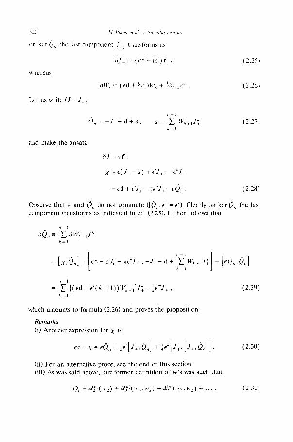
5•-• ~ = '~1. Batter el al. ,/ 3"inqtflar rector~

on kcr 0,, the last component ./ ~ t ransforms as

whereas

Le t us wr i t e ( J =- J . )

and make the ansatz

S f , = (Ed - . i E ' ) . f i ,

SW k = ( ed + k e ' ) W k + ~ o k , 2 e .

(2.25)

(2.26)

S f = , ¥ f ,

x = e ( J _ - a ) + E'J . - ½e"J+

ed + e'J 0 i ,,, e0, , (2.28) ~ - - - ~ E d + - - .

Observe that e and 0 , do not commute ( [ 0 , , el = e'). Clearly on ker 0,, the last component t ransforms as indicated in eq. (2.25). It then follows that

I1 I j k

sO, , = E a w k + , +

k - I

[ "' [ ] = [x,0, , ] = ~d+~'J.-'~"J= + , - J _ + d + E wk+,J~+ - ~0,,,0,, k=l

t l l

~_ .... , (2.29) = E { ( e d + e ' ( k + l ) ) W k + , } J k + + ~ e J+ k - I

which amounts to formula (2.26) and proves the proposit ion.

Remarks (i) Ano the r expression for X is

e d - x = e 0 , , + ½ e ' [ J + , 0 , ] + ¼e"[J+, [ J + , 0 , ] ] . (2.30)

(ii) For an alternative proof, see the end of this section. (iii) As was said above, our former definit ion of w's was such that

Q,, = AT' (w2) +A!~')(w3,w2) + A(~°(w4,w2) + . . . . (2.31)

n ]

Q,, = - J + d + a , a = ~_~ Wk+,Jk+ (2.27) k=l

M. Bauer et al. / Singular vectors 523

where w 2 - a2, zl~ n) maps ~ l - n ) / 2 ~ 5~n +~)/2 and A~ "), k >1 3, is linear in w k and

its derivatives. In the coordinate where w 2 - a 2 vanishes the explicit expressions become

AT)(0 ) = d " ,

~-k (k =

/ = 0

+I-1)(n ;k) ( 57, i--l i k >t 3. (2.32)

The relation between W's and w's (for k /> 3) is obviously independent of a 2 ~- W 2

(while w 2 = cqW 2) so we can set a 2 = 0 to compare them. As we saw,

w k = ~r k_ jW k 2 ~< k ~ 5, (2.33)

whereas for k >/6 there are additional terms on the r.h.s.. Direct computa t ion shows for instance that for n = 6

JW2~ w6 = 5!2(1416 + ~ 3 I (2.34)

while for n = 7

w6=12×5!2(W6 + ~ W 2 ) ,

w7 = 6!2(W7 + ~W3W4), (2.35)

and for n = 8

191 l,t/2 ] = 78 X 5 ! 2 [ W ~ + w6 I~Ns0 " 3 \ u l ,

( ,9 ) w 7 = 2 x 1 0 ! W 7+~.vW3W4 '

w 8 = 7! 2 + 6W3W~'- 7W; 2 + ~W3Ws + (41-W4) 2 , (2.36)

and so forth. These formulas are clearly invertible and it could well be that the Poisson structure expressed in this basis takes a more t ransparent form. The

maximal embedding of sl(2) in o ther simple Lie algebras is relevant in the construct ion of the corresponding W-algebras (see ref. [11]).

Proof of the formula for ~r k. Observe that by construct ion

°'k = tr(Jk-Jk+), (2.37)

524 .4,1. Bauer el al. / Singular cector,s

in the representa t ion of spin j. We set n = 2 / + 1 and define o-, = n. In t roduce the generat ing function

fl2k sin nO ~r(/3) = Y', k!~-T~/,,=tre/JJ el3S~= tre 2i°J,,

k = o sin 0 (2.38)

where 2 c o s 0 = 2 +/32. This last expression is obtained by using the structure of

the Lie algebra sl(2) or equivalently by looking at the 2 × 2 representat ion

e/J/ et~J+~ (2.39) /3 1+/3 2 "

Now sin nO/sin 0, the character of the spin-j representat ion, is a polynomial of

degree n - 1 in cos 0 and in view of the addition of angular momen ta fulfills

sin nO s in(n + 1)0 s in(n - 1)0 2 cos 0 - - - +

sin 0 sin 0 sin 0

From this relation we construct again a generat ing funct ion

s inn0 ~ ( t , c o s O = 1 + / ~ 2 ) = E tn I

n = 1 sin 0

1 1

1 - 2 t c o s 0 + t 2 ( l - - t ) 2 - - ~ 2

du ~ /32kuk

,,=1 2iTru" =j ( 1 - - + l ) ' (2.40)

SO that compar ing with the definition of o- k

o" k = k !2~ 2ircu"-k(1 -- U) 2(k+ I)

du (r = k ! 2 ~ - 2 i ~ . u ~ - k r~>>~O l'lr + 2 k + l )

2 k + l

(2.41)

as claimed.

M. Bauer et al. / S&gular cectors 525

An alternative proof is obtained by noting that the desired identity (2.23) is a

particular case of a more general combinatorial identity

l-p<~i<~n-k

which is readily proved by induction on p. Projectice connection and Gordan's "transeectant" formula*. From the work of

Janson and Peetre [13] one realizes that the construction of our original w-basis for

the ring R as well as the various differential polynomials in the w's giving again an element in R are parts of the same construction described as follows. Associate to a2(x) a projective connection b such that a 2 ( x ) - - - ~ n ( n z - 1)a(x) where the quantity a = b ' - ½b 2 transforms as a 2-differential with an added term equal to the schwarzian derivative. This enables one to define a covariant differential

D: f ~ - - - ) D f ~ + , , (2.43)

through D r = ( d - hb)f. For h = (1 - n ) / 2 the operator A2(a 2) is then given by Az(a2)f = D"f. With the notation

( r ) ~ = r ( r + l ) / r ( r ) = r ( r + 1 ) . . . ( r + l - 1), (2.44)

for the Pochammer symbol, Gordan 's " t ransvectant" [14] is then a map .~a ® .~r -~

• ~+~,+U such that if f ~ 5r~, g ~ .~-, then

F = Y'. ( - 1) t Dtg (2.45) /=0 (2A) N-! (2/Z)t '

belongs to "~+~,+U and depends on b only through the combination a. This is again proved by using the fact that under a variation 6b which leaves ot (hence w 2 = a z) invariant, one has (d - Ab)6b = (~b(d - (A - 1)b). Setting A = (1 - n)/2, /z = k a positive integer and N = n - k, we let g ---) w k and normalize the leading derivative of f to unity to obtain the other terms of our decomposition of the operator Qn in the form

,,-k (k

E l=o

( ~-~11~-1~ (Dtwk )D"-k- l f , (2.46)

as claimed in eq. (2.32). Similarly, given wk,w I ~ R (k, 1 positive integers), we

*The "transvectant" in Gordan's work is named "Uberschiebung".

52(~ M. Batter el al. / Singtdar i'ector~

obtain for each N >~ (t a map from R × R -~ R giving a k + l + N-differential. For instance for N = 1 it reduces to an example given in the text. It is interesting to note that in the context of automorphic forms Gordan's formula was rediscovered by Cohen [15] when restricted to PSL 2 transformations, a case where b vanishes.

Remark. As an alternative proof of proposition 2.1, one may consider tile operator

tl 1

0,, = - J + ( d - b J 0 ) + ~ Wt,+~Jk+, (2.47) k 2

where the Wk's are k-differentials. Define the n-dimensional vectors s ~= ( f j , . . . , f_ i ) v and / ) = (/~,0 . . . . . 0) v, where f_j is a - j-differential , and the other

are determined by the relation /~= ~),,]. Then )~ is a k-differential, and d - bJ~ acts as covariant derivative on J~, so that /~ is a j + 1-differential. The operator ~),, of eq. (2.24) is then obtained from 0,, by a gauge transformation

0,,, = e (h/2)J~ o n ( h / 2 } J + , (2.48)

provided W e = b ' /2 - b : /4 . This gauge transformation does not affect the compo- nents f_j and /~ and makes thus Q,, a covariant operator from ,¢(~, ,,~/_~ to

'~((I +n) /2"

3. A subfamily of singular vectors in Virasoro modules

The graded Virasoro algebra is generated by L .... m ~ 2, and a central element

(grade 0), such that

[L .... L,,] = ( m -n)L, ,~+,, + l c m ( m 2 - 1)6,,,+,,,,,, (3.1)

and c is understood as multiplying the identity operator in any representation (or

module) of interest. Consider the subalgebra B generated by L .... m >/0. Highest weight representa-

tions are characterized by a unique cyclic vector f (up to multiplication by a scalar) which carries a one-dimensional representation of B in the form (h is the

conformal weight)

L o f = h f , L m f = (I, m > 0. (3.2)

Verma modules are graded highest weight representations V(c, h) freely generated

by elements

fp,.p ...... ,,, = L p,L_,,~_... L p , f , 1 <~Pl <~P2 <~ " ' " <~Pk. (3.3)

M. Bauer et aL / Singular cectors 5 2 7

Finally singular vectors at level n arise from injective maps V(c, h + n) ~ V(c, h) where the image of the highest vector in V(c, h + n) takes the form

F = E Cp,.p. .... L , . .2 .... = 4 ~ ( L , . L _ 2 . . . . ) f P] + P 2 + - ." = n

(3.4)

satisfying therefore

L o F = (h + n ) F , L m F = 0 m > 0. (3.5)

Parametrize c, h and the positive integer n as follows, with j and j ' integers or

half-integers

c = l + 6 ( O + O - I ) 2,

h = - ( j O + j ' O - ' ) ( ( j + 1)0 + ( j ' + 1 ) o - l ) ,

n = (2 j + 1)(2j ' + 1), (3.6)

and 0 is any complex number, the values 0 and ~ being included in a limiting sense (for j ' = 0 and j = 0 respectively). Then a form of the Kac determinant formula is

Proposition 3.1. (Kac [1], Feigin and Fuchs [2, 16]). For c , h , n as aboce, V(c, h) admits a non-zero singular t'ector at lecel n and coneersely, all singular r, ectors are obtained in this way.

We emphasized above a notation involving spins j and j'. In terms of more familiar notations, with m a complex number

r = 2 j ' + 1, s = 2 j + l ,

m 6 t = O 2 = - - - - c = l

m + l ' m ( m + l ) '

( r ( m + 1) - s m ) 2 - 1 h = 4 m ( m + 1) , n = rs. (3.7)

Since the early investigations on the representation theory of the Virasoro algebra it has been a problem to give an explicit expression of singular vectors, namely of the polynomial ¢b(L_ l, L - 2 . . . . ), normalized by ~b = L~_I + . . . . For small values of j , j ' , one can obtain such expressions by brute force. The goal is however to obtain universal formulas.

528 M. Bauer et al. / Singular rectors

Let us first describe three general properties of singular vectors quoted by Feigin and Fuchs [16] with reference to work by Lutsyuk [17].

(i) The operator &(L) is a finite Laurent series in the variable t = 0 ~'. "['hen, as t tends to 0 or ~,

t--* 0 @, j ( L ) ~ I t ~2j+, , I ~ - ( 2 j ' + 1)1

[ . ~2i '+ 1 t - , ~ , 6j, j(L) ~L_~:j+~) (3.8)

A more precise form is t ~ O , ~j , . j (L)~(q~j,o(L)) 2j+l, t ~ , chj,.j(L)~ (~b0.j(L)) 2j'+ 1. Moreover (with the normalization & = L'_ 1 + . . . ) Feigin and Fuchs add the conjecture that under the transformation t - - - , - t , (hence c - - , 2 6 - c ) , L k ~ ( - 1 ) k- J L k, ~b(L, t) remains invariant.

(ii) For each positive integer k the subalgebra generated by L_k, L_k_ ~ . . . . is locally nilpotent. Let U k denote its enveloping algebra. We have a chain of

inclusions U ~ D U 2 3 U 3 . . . . It then makes sense to look at U_j m o d U 2 freely generated by L ~, U_ ~ m o d U 3 freely generated by L ~, L_ 2 considered

as commuting, U_ ~ mod U_~ isomorphic to the enveloping algebra of the Heisen- berg Lie algebra, e t c . . . (it would be interesting to analyze U ~ m o d U k in

general). Obviously & / , i ( L ) m o d U _ 2 is L'_ I. In U_ 1 m o d U _ 3 let ~.,i(L_l, L 2) denote the projection of &/.~ (with [L_ j, L_ 2] ~ 0). Then

~ ( L - , , L - e ) = I ~ (L2_ ,+4(MO+M'O ' ) 2 L _ 2 ) . (3.9) j<~M~< j

-j'~<M' <~j'

Of course M and M' range respectively over - j , - j + 1 . . . . . j and - j ' , - j ' + l, . . . . j ' . If the pair (M, M ' ) = (0, 0) is allowed it corresponds to a square. Otherwise (M, M ' ) and ( - M , - M ' ) give identical factors. Hence the right-hand side is a perfect square. Rational theories correspond to values of 0 such that there exist two coprime integers p and q satisfying

( p _ q ) 2

Oq + 0 - t p = 0, c = 1 - 6 (3.10) Pq

In the above formulas this may lead to the vanishing of some coefficients of L_e. (iii) The Virasoro algebra is a central extension of the algebra of vector fields on

a circle (c = 0), the Witt algebra, which admits representations on an infinite- dimensional vector space spanned by qJp, p ~ E of the form (A,/z arbitrary)

l_ktb p = [tz +p -- A(k - 1)] ~t,+ k . (3.11)

M. Bauer et al. / Singular t,ectors 529

For instance, on ~Op = 1 / z t'+~', 1_ k is r ep resen ted by - z - k ( z d / d z + A ( k - 1)).

U n d e r L _ k ~ l - k we have

~bj,.j(l_~, I_ 2 . . . . )~b 0 = q~f,j(A,/x)~O,. (3.12)

Set

A ( M , M ' ) = [ ( j + M ) 0 + ( j ' + M ' ) O - ¿ ] [ ( j + 1 - M ) 0 + ( j ' + 1 - M ' ) 0 - 1 ] ,

(3.13)

then

~,~(~, ~) = FI -j<M<j

-j'~M'~j'

[ (~ + A(M, M'))(tx + A ( - M , - M ' ) ) - 4 A ( M 0 + M'O-1) 2] .

(3.14)

Again the r ight -hand side is a perfec t square. These are, as far as we can say, all the known proper t ies of singular vectors in

the general case. Benoi t and Saint-Aubin [8], however, have found an explicit form in the case where j ' or j vanishes. This is the one we are about to exhibit here in a compac t form which bears some striking resemblance to our formula t ion of the

W-basis discussed in sect. 2. Such a resemblance does not come as a comple te surprise in view of the

following observat ion. In the limit where in eqs. (3.7) m ~ 0, hence c--* 0%

("classical l imit" [18]), the only values of h which remain finite cor respond to r = 2 j ' + 1 = 1. Let t ing n = s, this limiting value is (1 - n ) / 2 , which is the value of

the conformal weights of functions f discussed in sect. 2*. In this limit, it is suggested that the covar iant ope ra to r ~b mapp ing highest weight vectors f on their s ingular vector F should reduce to a covariant differential ope ra to r Q , mapp ing

"~(1-n)/2 onto "~(l+n)/2" The match ing is provided by the following identification:

L _ l ~ d ,

a(k- 2) - ~ , k > / 2 , ( 3 . 1 5 ) mL_k ( k - 2) !~r I

where ~r~ = n(n ~ - 1) /6 is the coefficient in t roduced in sect. 2. The form of the ope ra to r ~b is thus known in this limit: ~b = A~")(a2) and this suggests to recast the fo rm of ~b using the matr ix formal ism of sect. 2. Unexpectedly , but very fortu- nately, this matrix turns out to embody the whole form of ~b0j - beyond the limit rn ~ 0 - and enables one to r ep roduce the results of ref. [8].

* Letting m --* - 1 would lead to similar conclusions, with the role of r and s interchanged.

5 3 0 M. Bauer et al. / ,S'ingnlar t'ectors'

Let us concent ra te on the case r = 1, n = ~' = 2j + 1 as the other one is trivially related to it. So let once more

c = 1 3 + 6 ( t + t t ) ,

h = - j - t j ( j + 1),

n = 2 j + 1, (3.16)

where j = i .~ v, 1,~, . . . . In the Verma module V(c, h) we introduce a sequence of e lements denoted

f = f - J , f i+, . . . . . f~ , f i+ , = F , (3.17)

where f j is the highest weight state f,]).+~ is the singular vector F and )i~ ( j + M a non-negat ive integer) satisfies

L,, fM = ( h + j + M ) f M . (3.18)

We define the n-dimensional vectors

• . , J j ) , f : -

F = ( F , 0 . . . . . 0) T (3.19)

We also use the notat ion J+ introduced in sect. 2.

Proposit ion 3.2. (i) The equation

= _ L k__~(tJ+) k f (3.20) k = 0

defines F = f j + l as a non-l~anishing singular state at level n in V(c, h), i.e.

Lpf j+ , = 0, L , , f j + t = ( h + n ) f j + , . (3.21)

It 3p+1) 3p+, 1 p > 0 , L p f = J,, 2 - t - ~ - - 4 ( t J + ) P f " (3.22)

p > 0 ,

(ii) Moreover,

where

M. Bauer et al. / Singular cectors 531

Before turning to the proof let us make a few remarks. (a) The case r = 2j' + 1, s = 1 is simply obtained by changing j -->j', t ~ t - 1 (b) Comparing with the classical case in sect. 2 we find a similar operator with

k r dz -k d ~ L _ l , W k + l ~ t k L k_l-=t ~)~t Z T ( Z ) , (3.23)

Lp T ( z ) = E zp+2 (3.24)

p ~ Y

is the energy-momentum tensor. Thus the operator f ~ F reads

n-I dz z T ( z ) - J - + Y'~ ~ t ~ T ( z ) ( t z - ' J + ) k = -J-+~2-d- /~ (z - - -~+) " (3.25)

k = 0

It also follows from the above that if we express the differential operator Qn(W2 . . . . . W n) of sect. 2, without ever commuting d and the W's (i.e. without derivatives of W's), at the price of having W's inserted between d's, nor commut- ing W's among themselves, an equivalent form of the relation between F and f is

F = Q,(d ~ L _ , , W k ~ t k - ' L _ k ) f . (3.26)

(c) Eliminating all components fj, - j + 1 ~< k ~< j one finds the explicit form of the operator 05: f - f _ j ~ F

( n - 1 ) ! 2 - - r

05 -- Y~. t" lq r_ l t L_pr partitions of n i=lkPl + "'" +Pi)( n - - P l - "'" --Pi) L-p ' . . . .

n = P l + - ' - +P , - , P~>~ 1

(3.27)

which is the expression given by Benoit and Saint-Aubin [8]. We turn to the proof of the proposition and start with part (ii), since, as it will

emerge, it entails part (i). We note that the action of Lp o n f is in agreement with the commutation relations (p, q > 0)

[Lt,,Lq] = ( p - q ) L p + q ,

532 M. Bauer el al. / Singular t ectop:s

since

[L,,,c,,lf= J,, 2

3 p + 3 q + 1 = ( P - q ) J(I 2

= (p - q ) L p + q f .

( 3 p + 1 (1 + It -1) t"J'l+, J,, 2 - - ( 1 +½t '))tPJ(~l f

(1 + ½t-'))tP+qJP+~tf

(3.28)

Hence it is enough to prove it for L 1 and L 2. For L~ it reads component-wise

L I f M = ( t ( M - 2 ) - I ) ( j + M ) ( j + I - M ) f M _ ~ . (3.29)

This includes the case M = - j where the coefficient on the r.h.s, vanishes and

Ll f_ j= L , f =O (3.30)

by hypothesis, and if we extend it to M = j + 1 it will also imply L i ~+ J - LI F = 0.

Since f - ~ + l = L _ i f - j ,

L , f j+l = 2L, i f - j = - 2 j ( 1 + t ( j + 1 ) ) f ~, (3.31)

which agrees with the above formula for M = - j + 1. We can therefore assume the formula valid for M' ~< M ~< j and prove it for M + 1. By construction

j+M

fM+t = E L - l - k f M - k t k ( J k + ) M , M k ' ( 3 . 3 2 ) k=0

while from the recursion hypothesis

M'<~M, L,fM,= ( t ( M ' - 2) - 1)(J+)M,.M,_,fM,_ , . (3.33)

Using for k>~0 L 1 L l - k = ( 2 + k ) L - k + L - t - k L I we find

j+M

L,fM+,= E ( 2 + k ) L * * _,h,_,t (J+)M,M-, k =0

+ j + M - I

E k =0

_ e tk tJ k+l , (3.34) ( t ( M - k - 2 ) - I ) L ,-kJM-k ~. + )M.M-k-,

M. Bauer et al. / Singular vectors

where we use the structure of the matrix J+ to identify

= ( l k + l $ ( J k ) M , M - k ( J + ) M - k , M - k - 1 \~+ ] M , M - k - I "

533

(3.35)

Hence splitting the first sum into the contribution k = O, k > 0 and adding the

second term we get

j + M

fM Y'. j k - , , = L-kfM-k( + )M-I,M-k (3.37) k = l

and using the same property of J+ we find

LIfM+ ~ = {2L 0 + ( t (M+ 1) - 1)(J+)M.M_~}fM. (3.38)

Explicitly the bracket reads

2 M - 2tj(j + 1) + ( t (M+ 1) - 1 ) ( ( j - M + 1 ) ( j + M )

= ( t ( M - 1) - 1 ) ( j - M ) ( j +M+ 1), (3.39)

i.e. the formula is valid for M + 1 if it is valid up to M. A similar argument applies to the action of L 2 which is supposed to read

component-wise:

L2fM = [ t 2 ( M _ 7) _ 7t](j(j + 1) - M ( M - 1 ) ) ( j ( j + l) - ( M - 1 ) ( M - 2))fM_ 2.

(3.40)

This includes the cases Lzf_i=Lzf_j+ ~ = 0 valid by hypothesis. Again let us assume the formula true for M' ~< M and let us establish it for M + 1. We use for k>_-0

1 LzL_~_k=(3+k)Ll_~+L_~_kLz+-~6~,~(13+6(t+t-~)), (3.41)

and start from

j + M

fM+I=L-IfM+L2fM-jt(J+)M,M-I + E L-l-kfM-ktk(Jk+)M,M-k. (3.42) k = 2

Recognizing that

j + M k L,fM+ l=2LofM+ ~, ( t (M+ l/-1)L_kfM_kt*- '(J+)M.M_ k. (3.36)

k = l

5 3 4 M. Bauer et al. / Singular rectors

From the recursion hypothesis,

L 2 f M + , = 3L,. [ I~, + t[4L,, + }(13 + 6(t + t ' ) ) ] f . , t - , ( J + ) M . , , , ,

+ j + M

E k = 2

(3 + k ) L , _z:fm_/.t~(J+)M.M k

+ j + M - 2

Y'~ L_ l ~fM_k_2(t2(M--k--7)--7t) tk(Jk++2)M.M__k_ 2. (3.43) k =0

We take into account the expression for L , f M obtained above to rewrite

L2fM+ , = [3( t( M - 2) - l) +4t(M-l)-4t2j(j+l)+#t+3t2+3]

x ( j ( j + 1) - M ( M - 1))fM_ ,

+ j + m - 2

E k = (}

7 7 )L " k k+2 (3.44) -k~M-2-k t (J+ )M.M 2-k" ( t 2 ( 5 + M - ~ - z t ,

Comparing with

j + M - 2

fM- , = E L ,_kfM_2_ktk(J+)M 2, M 2 k ' (3"45/ k =0

we get

where the factor A is

L 2fM+~=AfM , , (3.46)

A = t ( j ( j + 1) - M ( M - 1 ) ) { 3 ( M - 2) + 4 ( M - 1) - 4t j ( j + 1)

3 7 + #_ + 3t +j( j + I) - ( M - I ) (M- 2)}(t(M + 31 - ~), (3.47)

and after some rearrangement

A = (t2(M - ~) - 7)(j(j + ]) -M(M+ ] ) ) ( j ( j + I) -M(M- I)). (3.48)

This proves the formula for L2fM+ I. As above the induction holds up to M = j in which case we obtain

L2f j+ i ~ L2F = O, (3.49)

M. Bauer et a L / Singular vectors 535

thus completing the proofs of parts (i) and (ii) of the proposition. Obviously F 4:0

since the coefficient of L " , is 1. Let us conclude by a few observations. (a) If we rescale the components of f through

tj+m~ [ IM+j~ fm =" JMW+ Im.-2, - j ~ M < < . j , (3.50)

the "descent" equation reads for p >~ 1 and - j ~< M ~<j

' -1)) " L p f g = M - 3 p + l ( l + 2 t fM-p , 2

(3.51)

to be compared with the representation of the Witt algebra recalled above in eq.

(3.11),

l p q J r = ( I x + r + A ( p + l ) ) O r _ p , r , p ~ Z . (3.52)

Here the grading is through integers shifted by/z, but an integral shift allows us to

"S take/~ mod 1. Thus the action of LR on f , restricted to p >t 1, can be identified with the one of lp, provided

1 - - I - - 1 A = - 3 ( l + ~ / ' ) , / z = ( j + l + ~ t ) m o d l , (3.53)

and of course these formulas hold with t ~ t - I for the other series of singular

vectors r = 2j ' + 1, s = 1. A natural explanation for the origin of these descent equations will be provided in sect. 5.

(b) In the case r = 1, s = 2j + 1, we see that as t ~ 0 or ~ the singular vector

F = f b ( L ) f (3.54)

behaves as

t--'-~0, ~ ( t ) ~ (L i) 2j+l,

t --* oo, 4)(L) ~ t2JL2j+ l,

as expected (with t o t - l, 0 o oo and j <-,j' in the case r = 2j ' + 1, s = 1). More- over the conjecture of Feigin and Fuehs is verified: in both cases, ~b(L) is invariant under t ~ t - 1, L -k ~ ( - 1) k- IL -k.

(c) Let us look at ~b(L) mod L_3, again for r = 1, s = 2j + 1, assuming therefore

[ L _ j , L _ : ] ~ 0 .

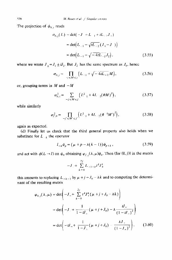
5 3 6 M. Bauer et al. / Singular vectors

The projection of Oo.j reads

0-o.i(L) = det( - J +L_ j + tL 2J+)

=det(L- . l + tv/~-2(J+ - J ))

= det( _, + ¢ - 4,L

where we wrote J+=Jl ±/,]2. But J2 has the same spectrum as Jo, hence

0-,,,i = I-I . (L , + ~ Z 4 t L _ 2 M ) , -j<~M<~j

or, grouping terms in M and - M

while similarly

0 -2 = +4L_2(OM)2) , 0.j E (L2-1 -j<~M<~j

%.,2 o = I-I ( L2- , + 4L 2(O-'M') e) -j'<~M'<~j'

(3.55)

(3.56)

(3.57)

(3.58)

this amounts to replacing L_ k_ ~ by/z + j +J0 - Ak and to computing the determi- nant of the resulting matrix

¢o,j(A,/z) --- det - J _ + Y'~ tkJk+ ( Iz + j + Jo - Ak) k = 0

1 d+ ) = d e t - J _ + 1-tJ------f ( ~ + j + J ° ) - A ( 1 - ~ + ) 2

1 = det - t J _ + 1 -J----~

(/z + j +Jo) A J+ ) (1 ~ j + ) 2 , (3.60)

- J _ + 2j ]~ k k L_l_k t J+

k = 0

and act with ~b(L ~ l) on 00 obtaining ~/,~(h, ~z)0n. Then (for (0, j)) in the matrix

(3.59) l kqJ p = ( I x + p - A ( k - 1 ) ) O p + k ,

again as expected. (d) Finally let us check that the third general property also holds when we

substitute for L_k the operator

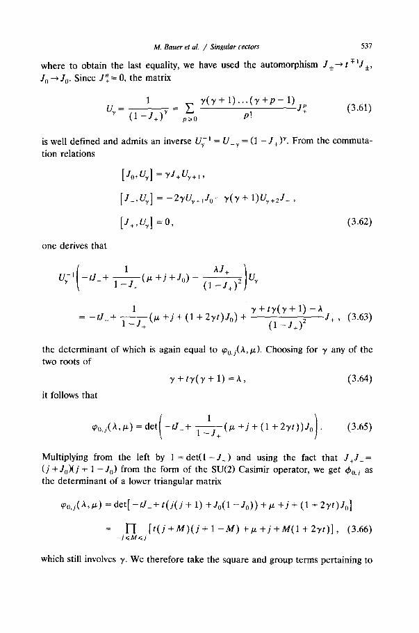
M. Bauer et al. / Singular vectors

where to obtain the last equality, we have used the automorphism J + - 0, the matrix Jo --" J0. Since " -

537

J ± ~ t:~lJ +_,

1 y ( y + 1 ) . . . ( y + p - 1) Uv= ( 1 - J + ) V = E P! JP+ (3.61)

p~>0

is well defined and admits an inverse Ur -I = U_v = (1 - J + ) L From the commuta- tion relations

[Jo,Oz,] = T J + U ~ , + I ,

[J ,O~] = - 2 T V ~ + , J o - y ( y + l)Uv+zJ+,

[J+,Uv] = 0 , (3.62)

one derives that

1 A J+ ) U; t - tJ_+ 1 -J----~(g +j +Jo) (1 _ j+ )2 U~,

1 = - t J _ + q---S---, (/-* +J + (1 + 2yt)Jo) +

l - s +

y + t y ( y + 1) - A

(1 _j+)z J + , (3.63)

the determinant of which is again equal to ~o.~(A,/2,). Choosing for y any of the two roots of

3' + ty (y + 1) =A, (3.64)

it follows that

( 1 ) ~o,~(A,g) = det - t J _ + 1- - -~+(g + j + (1 + 2 7 t ) ) J 0 . (3.65)

Multiplying from the left by 1 = d e t ( 1 - J + ) and using the fact that J+J_= (J +Jo)(J + 1 -Jo) from the form of the SU(2) Casimir operator, we get ~bo, j as the determinant of a lower triangular matrix

~o,i(A,~z) = d e t [ - t J _ + t ( j ( j + 1) +Jo(1 - J o ) ) +ix + j + (1 + 2yt)Jo]

= I--I [ t ( j + M ) ( j + l - M ) + ~ + j + M ( l + 2 y t ) ] , (3.66) -j~M<~j

which still involves 3'- We therefore take the square and group terms pertaining to

538 M. B a u e r et al. / S ingular rectop:v

M and - M to get after some algebra using eq. (3.64) the desired result

~ { . i ( a , g ) : 1--I { [ g + ( j + M ) ( I + ( j + I - M ) t ) ] j ~ M < j

× [ / ~ + ( . / - M ) ( 1 + ( j + l + M ) t ) ] -4AM2t} (3.67)

independent of the choice of the root in (3.64). We have thus verified the property (3.14) whenever j or j ' vanishes. This is all

we shall need in sect. 5 in the construction of the general singular vectors.

4. Fusion

To prepare for the computation of general singular vectors, we describe in this section the fusion of highest weight modules, introduced by Belavin et al. [3] as an appropriate adaptation of the notion of tensor product decomposition.

We fix throughout our discussion the central charge c and attach isomorphic Virasoro algebras to each point of the Riemann sphere and similarly heighest weight modules also parametrized by a point with coordinate x. To the latter we let correspond primary chiral fields f l , (x ) and their descendents. We refer to a finite non-decreasing sequence of positive integers 1 <~r~ <~r 2 <~ . . . <~r k as a Young tableau Y, with IYI = rj + r 2 + . . . + r k and write

L , . . . . L ,. - L v ' (4.1)

Let T ( z ) stand for the energy-momentum tensor. The descendents of fh(x),

L v f h ( X ) ~ L vlc , h ; x ) , (4.2)

where it is understood that one operates with the Virasoro algebra at x, are obtained by applying repeatedly the short-distance expansion of T with the field fh and its descendents. On the primary field, it reads

T ( ~ ) f h ( x ) = ~ ( ~ - - x ) " - 2 L _ n f h ( x ) , (4.3) n = 0

with

d L o f j , ( x ) = h f h ( X ) , L , f h (X ) = ~ x f h ( x ) , (4.4)

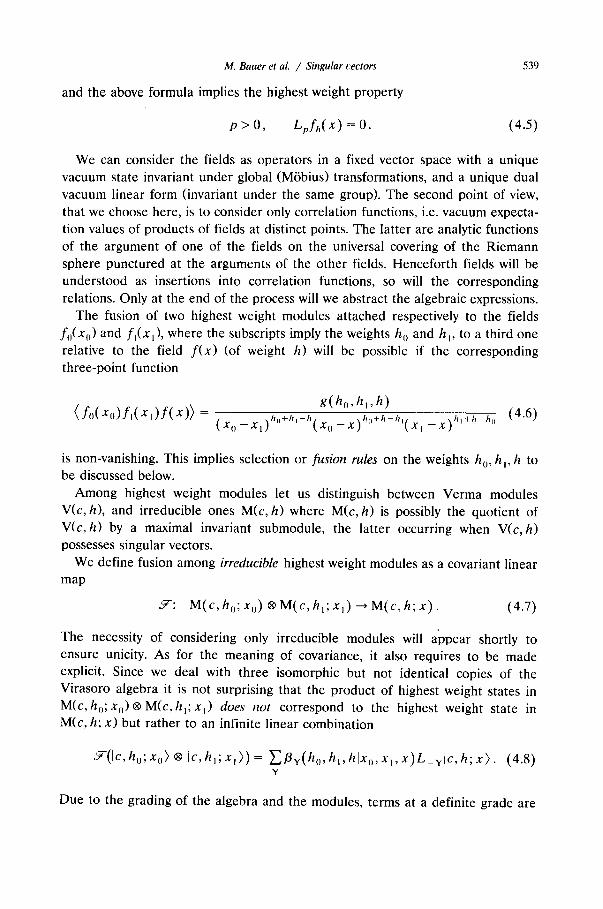
M. Bauer et aL / Singular vectors

and the above formula implies the highest weight property

539

p > O, Lpfh(x ) = O. (4.5)

We can consider the fields as operators in a fixed vector space with a unique vacuum state invariant under global (M6bius) transformations, and a unique dual vacuum linear form (invariant under the same group). The second point of view, that we choose here, is to consider only correlation functions, i.e. vacuum expecta- tion values of products of fields at distinct points. The latter are analytic functions of the argument of one of the fields on the universal covering of the Riemann sphere punctured at the arguments of the other fields. Henceforth fields will be understood as insertions into correlation functions, so will the corresponding relations. Only at the end of the process will we abstract the algebraic expressions.

The fusion of two highest weight modules attached respectively to the fields fo(xo) and f~(x~), where the subscripts imply the weights h 0 and hI, to a third one relative to the field f (x) (of weight h) will be possible if the corresponding three-point function

( k,( xo)f|( X, )f(X)) = g(ho,hl,h)

( X 0 -- x l ) h° +hl - h ( Xo -- x ) ho + h - h l ( x l _ x ) hl + h - h o (4.6)

is non-vanishing. This implies selection or fusion rules on the weights h0, h~, h to be discussed below.

Among highest weight modules let us distinguish between Verma modules V(c, h), and irreducible ones M(c, h) where M(c,h) is possibly the quotient of V(c,h) by a maximal invariant submodule, the latter occurring when V(c,h) possesses singular vectors.

We define fusion among irreducible highest weight modules as a covariant linear map

.~-: M ( c , h 0 ; x 0 ) ® M ( c , h , ; x , ) ~ M ( c , h ; x ) . (4.7)

The necessity of considering only irreducible modules will appear shortly to ensure unicity. As for the meaning of covariance, it also requires to be made explicit. Since we deal with three isomorphic but not identical copies of the Virasoro algebra it is not surprising that the product of highest weight states in M(c, ho;xo)®M(c, h6x~) does not correspond to the highest weight state in M(c, h; x) but rather to an infinite linear combination

9-(Ic, ho;xo)® lc, h~;x,))= Y'.~y(ho,h~,hlxo,xl,X)L_yIc, h;x ). (4.8) Y

Due to the grading of the algebra and the modules, terms at a definite grade are

540 M. Bat¢er et al. / ,S'ittgu&r i'ec'torv

well defined and convergence is understood in this weak sense. Part of the

definition of fusion involves the determination of the coefficients /3Y. To obtain them and give a precise description of the correspondence ,Y, a disguised formula- tion of chiral vertex operators [19], we rely on Wilson's short-distance expansion of products of fields as a heuristic guide.

Let us choose the coordinates in such a way that

' ( 4 . 9 ) X o = X + ~Z, Xl = X - - ~-Z.

This is not a serious restriction since global conformal transformations act transi-

tively on triplets of points. As z ~ 0 the product of fields fo(xo)fl(xj) (inserted in correlations) is equivalent to a sum of expansions of the form

{ g(ho,hl,h) fo(xo)f,(x,) ~ ~ zh,,+h,-h

17

~zlVt/3v(ho,h~,h)Ly yfh(X)}. (4.10)

I As was mentioned above the choice of the mid-point x = 5(xo + x t ) is by no means mandatory and could well be modified using

fh(X +X')=exp(x'L ,)fh(X), (4.11)

without changing the structure of the above expansion. It has however, the virtue

that the coefficients satisfy the symmetry property

/ 3 v ( h o , h , , h ) = ( - l)lVt/3v(h , ,h o , h ) , (4.12)

disregarding a global phase arising from the prefactor z h' '+h'-h, conveniently

absorbed in the normalization. The covariance of .~ which will allow us to compute the fl 's consists in the

following requirement. Consider a holomorphic univalent map x - ~ 2 = g ( x ) in a common neighborhood U of xo, x~,x giving a one-to-one map U~,g(U). We require that Wilson's expansion be such that both sides have identical transforma-

tion properties. Namely if

¢}(xi)dx~', = j~(2,)"Ox,'h' (4.13)

we impose that the coefficients /3 v appearing in the expansion of fo(X())//fl(Xl ) in terms of the descendents of f((x o + x l ) / 2 ) be the same as those appearing in the corresponding quantities with tildes. The univalency of the map g is a weak requirement since we only need a pair of points xt~, xl -~x, so U can be shrunk at will and the condition reduces to g ' 4:0 at the common limiting point. We will see below how one applies this principle in practice to compute the coefficients /3. We

M. Bauer et al. / Singular cectors

can thus define the map 5 r on M(c, ho; xo)® M(c, h6 xj) by the rules

541

1 ,~lc, ho; Xo) ® IC,hl; xl) - zh.+h,_h Y'~zlVll3vL-vlc,h; x),

Y

(4.14)

~-(L_p® 1) (--1) p z p h l ( P _ l ) + _~L_ l -Z-~z + ~ k+P-Zk L -P-k ' k >/0

(4.15a)

[ d I (z)k( 1 z -Z z + E ~r(l®L_p)-- ~ h o ( p - 1 ) - ~ L _ l T k > 0

k +p - 2 ] tL_p_k k

o

(4.15b)

Remarks (a) For p = 1 in both (4.15a, b)the last sums reduce to L_ l (formally (-~)) = 1)

so that they read

d L_ 1 .~-(L_, ® 1) = ~z + ~ - - '

d L - |

,~'(1 ®L_I) = - d----z + ~ (4.16)

(b) The expressions in (4.15) follow from the Ward identities [3]* for the insertions of energy-momentum tensors T(~I)... T(,~ k) into correlation functions, in combinations with short-distance expansions for products of the form T(~)fi(x ~)

( ( L_R ... L_p,fo( Xo) ) f ,( x , ) ... ) = ~LP_p,( X,,) .. . 2_p,(Xo) ( fo(Xo)f l (Xl) . . . ) ,

(4.17)

w h e r e the d i f f e r e n t i a l o p e r a t o r S e p r e a d s

~-, ( ( P - 1)h i -~ -p ( Xo)

t ( x i - x o ) p

1 a 1 ] (4.18)

( X i - - X o ) p- I ~X i "

Once we have obtained the expressions for the singular vectors, eqs. (4.17) and (4.18) will enable us to translate them into partial linear differential equations satisfied by correlation functions involving the corresponding primary fields.

* This was also discussed in ref. [20]; the calculation of the coefficients 13v presented in appendix A of that reference was, however, incorrect (but this did not affect the bulk of the paper). The following discussion gives the correct and systematic way to carry out these calculations.

542 M. Bauer el al. / Singular ~ ('cmr~

Each ~, is expanded for x o ~ x in the form

.'.~' p (xo) = ( - l / z ) " ( ( p - 1)h I + ~ z d , - ~ k > 0 k

x Y' ( - 1 ) v+k h i ( P + k - l ) l ] ,j,+k + ,p+k_lai , (4.19)

i>2 ( x - x ~ ( x - x ~ J

and the last sum is identified as L_p_ k. This is then iterated to get the general case. For the (locally nilpotent) subalgebra generated by the L_p'S (p > 0) the map 9- does not involve the central charge and 9- defines an isomorphism in the sense

that

[ g ( L _ , , , ® 1 ) , ~ ( L , ,®1)] = ( m - n ) g ( L _ , , , _ , , ® l ) (4.20)

with m, n > 0, and similarly with x o ~ x~. (c) One passes from (4.15a) to (4.15b) by exchanging h 0 ~ h I, z ~ - z , with x

left invariant. This justifies our symmetric t reatment in the general discussion.

(d) In the coinciding point limit, i.e. as z --) 0, we have

lim z "~(zh~'[c, h o ; x o ) ® z h ' [ c , h l ; x , ) ) = ] c , h ; x ) , (4.21) z - + O

obtaining therefore the highest weight vector in M(c, h; x). This is compatible with

the transformation properties of the fields since (x o - x ~ ) h f ( ( x o + x~)/2) behaves as d x h f ( x ) as x o - x I --+0. It shows moreover that the leading term in the

short-distance expansion of two primary fields (corresponding to highest weight modules) is always a primary field (for the Virasoro algebra), a fact that we will

recover and use later on. A particular case of fusion occurs when two fields are identical. We normalize

the two-point function ( f ( x ) f ( y ) ) to (x _y) -Zh . The identity or vacuum sector (h = 0) occurs in the short-distance expansion of the product f ( x ) f ( y ) . Since on the Riemann sphere the value ( T ( ~ ) ) = 0 is the only one compatible with the

invariance under global conformal transformations, we find from the above, with

x ' - - ( r - 1 ) h - X ~ x x , (4.22)

1 ( ( c _ , , . . . . . .

( _ 1 ) ~', - xT#+-27 ~ [(r , + l )h + r 2 + . . . +rk]

X [ ( r 2 + 1 ) h + r . ~ + . . . + r k ] . . . [ ( r k + 1 )h] . (4.23)

M. Bauer et al. / Singular cectors 543

On the other hand, normalizing the fields in such a way that g(h o, h 1, h ) = 1 we have from the three-point function

( fo( xo) f , ( x, ) f(O)) = +

1 ~ ( z I" ( -1)q zh°+hl-hx2h Y l "~X ] E p!q]

= ) p+q=n

r ( h , - h o - h + 1) r ( h o - h I - h + 1)

r ( h , - h o - h + 1 - p ) r ( h , , - h , - h + 1 - q )

1 Z,,,,+h,-h ~' . , zm/3v((L-v f (X)) f (O)) •

Y (4.24)

By comparison we get the sum rules on the coefficients /3Y,

E 1 ~ r I ~ < r 2 . . .

r I + r 2 - t - . . . = n

[ ( r , + l ) h + i>_.2~ri][(r2jt + 1)h + i~3 y'~ ri] "''/3r''r2 ....

1 1 F ( h t - h o - h + l ) F ( h o - h ~ - h + l ) = 2,-- 7 ~ ( - 1 ) P p ! q ! F(h - h o - h + l - p ) F ( h o - h , - h + l - q )

p + q = n

(4.25)

In particular for IYI = 1 this fixes /3~ through

2h/31 = h 0 - h i , (4.26)

while for I YI = 2 we get the relation

h ( h o - hi ) 2 2h(2h + 1)/3,., + 3h/32 = ~ + 2 ' (4.27)

and so on. By examining further sum rules, starting more generally from

( f o ( x o ) f , ( x , ) ( L - y f ( O ) ) ) ,

one would obtain an infinity of linear systems determining the coefficients/3 v. The above method is equivalent to (but less effective than) the one following

from the covariance principle. Let us show this explicitly by comparing the

544 M. Bauer et al. / Singular I cctor.s

transformation properties of both sides of the short-distance expansion. With the notations introduced above we require that

1 zh,,+h,_ h ~zJYI/3y(L y f ) ( X )

Y

1 1 ~dx,~ ~ x l ] (20_2,)h"+"'-h v ~ ( 2 " - ' r ' ) l v l / 3 v ( L - v f ) / ~ '

(4.28)

i i where as before x o =x + 5z, xl = x - 5z and

( g _ y f ) ( ~ ) = g _ y e x p 2°+2~2 2)L_l]f(2) . (4.29)

We need here the transformation properties of the descendent fields (Lv f ) ( x ) with f primary. The easiest way is to apply the above formula in infinitesimal form. Set

; = y - e ( y ) . (4.30)

Eq. (4.28) reduces to

O 0 } 1 - - +h,e'(x,) +e(x,)~x 1 Z,,,+h,_ h Y'.zlVl[JvL_vf(X) h°e'(x°) + e(x°) Oxo v

1 zh,,+h- h EzlVl~y6~[L_yf(X)]. (4.31)

Y

Choose

so that

e(y) =ek(Y--X) k+', k>~ - 1 , (4.32)

6~L vf(X)=EkLk L vf (X) . (4.33)

The covariance condition becomes, with k >t - 1,

[ (z), (z~k+,{, ~ l~ 0 Lk-- 2 (k + l)(h°+(-1)kh')- 2 2 Ox + ( l + ( - - 1 ) k ) ~ z

X m 1

zho+h,-h ~-"ztYI[JyL- y f ( x ) = O. Y

(4.34)

M. Bauer et al. / Singular t'ectors 545

Since L t and L 2 generate by commutators the complete algebra of Lk's, k ~> 1 (recall that Lk+ 2 = ((-1)k/k!)(ad LI)kLz) it is sufficient to impose the two rela- tions pertaining to k = 1 and k = 2. For notational simplicity define

f¢v)= ~' ~ v L _ v f ' p>lO, ( 4 . 3 5 ) IYI=p

where f~0) is equal to f . The above translates into the conditions

I I f ( P - 2 ) Lif~P)= ( ho - h]) f~v-I) + ~L_ (4.36a)

h + p + 2 ( h 0 + h i - 1) L2f(p) = f(p-2) . (4.36b)

4

It is understood that f (P) vanishes if p < 0. As a consequence, we recover the fact that f~0) _ f is a highest weight state (or primary field) as already claimed. Let us exemplify on the first few values of p how these equations determine recursively the coefficients/3 v assuming M(c, h; x) irreducible and the fusion rules (specified below) satisfied.

With f ~ l ) = / 3 j L ~f the first equation gives as before

For p = 2,

1 2 h / 3 , = h o - h , ~ / 3 , = ~ ( h , , - h , ) i fh4=O. (4.37)

we get ~om eq. (4.36a)

f~2,= ([3,.,L2_, + ~2L_2) f '

h (h 0 - h i ) 2 2 h ( 2 h + 1)/3t, l + 3h/32 = ~ + 2 '

(4.38)

(4.39)

as before, while eq. (4.36b) yields

h h o + h l 6h/3,. l + (4h + ½c)/3~ = ~- + ~ (4.40)

Provided the determinant

K z =h (16h 2 + 2 h ( c - 5) + c ) (4.41)

546 ).I. Bauer cta/. / Sm'.'u/ar lcctor~

is different from zero, we obtain, denoting h 0 +/ l I = s and h¢~--111 d,

For p = 3

2hZ+h(c - 12s+ 16d 2) + 2 c d -~

/-~1.1 = 8h[16ha+2h(c_5)+c] (4.42a)

.[°'=(~,.,.LL3 ,+[3,.2L ,L 2+~3L 3)]'. (4.43)

Again provided

K3=h(16h2+2h(c-5) + c ) ( 3 h 2 + h ( c - 7 ) + c + 2 ) (4.44)

is non-vanishing, we find, with the help of a computer,

~1.1.1 = {d( 18h3 +h2( 48d: - 108s + 15c + 18)

+ h ( 8 4 s - 36cs + 22cd 2 - 52d 2 + 3c 2 - c - 20)

+2c2d 2 + 16cd 2 + c 2 - 12cs + 2c)}

× [48h(16h 2 + 2 h ( c - 5 ) + c ) ( 3 h 2 + h ( c - 7 ) + c + 2 ) ] i, (4.45a)

~1.2 = {d( 3h4 + h3( 6s + c - 16) + hX(2cs + 9s - 9d 2 - 2c + 9)

+h(3sc- 9 s - 3cd 2 + 7d 2 - c) + c ( s - d2))}

×[2h(16h2+2h(c-5) +c) (3h2+h(c -7 ) + c + 2)] - ' (4.45b)

d ( h ( s - 1) + s - d 2)

/33 = 2h(3h z + h(c - 7) + c + 2) " (4.45c)

The method determines recursively fcP~, the component at level p, by solving at each stage a P(p) × P(p) linear system, with P(p) the number of partitions of the integer p. The determinant of this linear system is nothing other than the Kac determinant at the corresponding level. If the complete determinant does not appear in some of the above expressions, this is due to cancellation of factors

between numerator and denominator.

h 2 + h ( 2 s - 1 ) + s - 3 d 2

/32= [16h2+Zh(c-5) + c ] (4.42b)

M. Bauer et al. / Singular cectors 547

If M(c, h) = V(c, h), i.e. if V(c, h) is irreducible, or equivalently does not possess

singular vectors, no Kac determinant vanishes and the coefficients /3 v are deter- mined from eqs. (4.36) for arbitrary h~j, h~. On the other hand, assume that V(c, h) is reducible, i.e. M(c, h) is obtained by quotienting V(c, h) by invariant submodules arising from singular vectors annihilated by L k, k > 0. When attempting to solve the system (4.36) at level p or higher, where p is the level of this singular vector, one can at best hope to determine f(P) Up to this singular vector or its descen- dents. This is why we defined fusion among irreducible modules, so that in M(c, h) we work modulo singular vectors and descendents. In other words, the latter can be set equal to zero. Still we have to make sure that the right-hand side of the corresponding linear system lies in the range of the linear operator on the left. This imposes conditions on the triplet hl~, hi, h as necessary ones for fusion. We thus obtain fusion rules.

This is already apparent at level 1, where the Kac determinant reduces to h. From 2h/3~ = h o - h ~ it follows that if h vanishes we must have h 0 = h~. Thus two modules can have the vacuum (h = 0) sector in their fusion rules only if they have equal weights, a well known property which entails that the only non-vanishing two-point functions of primary fields are those involving fields of equal weight.

Descendents of a singular vector at level p manifest themselves by the vanishing of the Kac determinant at level p' > p. Consistency requires that for this value of h, the right-hand side of the linear system continues to lie in the range of the linear operator on the left for the same values of h o and h~. For instance, keeping h = 0, the equations at level two read

( h 0 - h l ) 2 0 2 ' CI~2 = h° + hI ' (4.46)

We recover consistently the condition h o = h ~ and, assuming c ~ 0 , we find

]~2 = ( h 0 "1"- h¿)//c. This leaves /31, i arbitrary. But in the irreducible module M(c, 0) one quotients by descendents of the singular vector L ~ic, 0) ~ V(c, 0), and a term like /31, i L 2_ l lC, 0) can be ignored.

Let us look at a further example, assuming V(c, h) degenerate at level two, i.e.

16h 2 + 2 h ( c - 5) + c = 0. (4.47)

The fusion rules then require that

(h o + h , ) ( 2 h + 1) - 3 (h o - h , ) 2 + h ( h - 1) = 0. (4.48)

548 M. Bauer et al. / Singular cectors

Assume for simplicity that h 4= - 1 (i.e. c ~ ~, the "classical" case). Solving for c

and s = h 0 + h I (with d = h 0 - h I ) we get

3d2 -h (h - 1) - 16h2 + 10h

s = 2h + 1 ' c = 2h + 1 (4.49)

At level 2 we find

h + 2 d 2 [ 3 L2 ] f~2) 8h(2h + 1) L2-1f+/32 L-2 2 ( 2 h + 1 ) - t f , (4.50)

where the factor of the arbitrary coefficient /32 is the singular vector in V(c, h) set equal to zero in M(c, h). At level 3 we then find the consistent expression

30h 3 + (20d 2 - 17)h 2 + (14d 2 - l l ) h + 20d 2 - 2

fO)=d L~, 4 8 h ( h + 2 ) ( 2 h - 1 ) ( 2 h + l ) ( 5 h + l )

h 2 _ d 2

+L-~L-2 h(h + 2)(2h - 1)(5h + 1)

h2-d2 }

- L - 3 2h(2h - 1)(5h + 1) f

I 3L2] +~22(h+2) L - ' L-2 2 ( 2 h + 1 ) - ' f (4.51)

which involves the first descendent of the singular vector at level 2 multiplied by

the same arbitrary coefficiency /32. The latter vanishes in M(c,h) . Note that ( c = - ~ ) one should also take care of the particular beyond the case h = - 5

I ( C ~ - - 2 2 I I T), h = - 2 ( c = 2 8 ) and h = ( c = 2). The last one is the cases h = - ~ 5 familiar case of the (chiral part of the) Ising model if we assume h 0 = h I = h(1 - h)/2(2h + 1). Then the fusion rule of the spin operator (~r: h~. = l ) reads

~r~r ~ 1 + e (4.52)

with E the energy operator (h~ = ½). In order that fusion be uniquely defined (up to overall normalization) it was

required that the target module M(c, h) be irreducible, but we did not yet use the irreducibility of the initial modules. In sect. 5 we will examine the consequences of quotienting by descendents of singular vectors in the initial spaces.

M. Bauer et aL / Singular cectors 549

Remark. In applications it might be more convenient to use one of x 0 or x~ as fusion point. For instance if x---x~ then with x 0 = x +z , Xl = x we write

9-1c, h0;z + x ) ® Ic, h l ; x ) = - - 1

zh,,+h,_ ~ ~ z l V l f l v L _ v l c , h ; x ) , (4.53) Y

'gr(L-p ®1) ( - 1 ) n [ d ] = - - hi( p - 1) + z L _ l - Z - ~ z +

z p y" z k ( k + p - - 2 ) L _ n _ k ,

k>~o k

(4.54a)

11 o] .7(1 ®L_p) = z-7 h(,(p - 1) -z-d-~z + L _ n , (4.54b)

and ~ ( L _ 1 ~ I) = Oz, Y-(1 ~ L _ l ) = - - 0 z "Jr L _ ~ while covariance reads

1 [ L k - ( h ( , ( k + l ) z k+zk+'az)]zh .+h,_h ~'~ z n f ( n ) = 0 ,

p>~O

i.e.

L l f tp)= ( p - 1 +h +h o - h l ) f in-l)

(4.55)

(4.56a)

L 2 f (p )= ( p - 2 +h + 2h o - h l ) f (p-2) (4.56b)

5. General singular vectors

Our final goal is to obtain singular vectors in a Verma module V(c, hj , . j ) f r o m

fusion, using the explicit expressions of sect. 2 for the particular cases hj,,o and ho, j. Before we proceed, it is good to have some examples obtained by direct computation. We give two of them.

Example 1. Singular cector at level 4 for h ~, ~ = - ¼(t + t - i + 2). Set

~-+_=t+t -I + 2 , (5.1)

so that h~,k= 3 - ~-+. The singular vector is obtained by applying the following operator to the highest weight state:

3 2 3 z L_2+ _~._L_2L_ 1 ~b, ½ =L41 +~'+~" L2_2 + ~ ' + L _ l

- I ( ¢ + + ¢ _ ) L _ t L _ 2 L _ I. (5.2)

One can attempt to recast this in matrix form. One possibility is as follows. Write

F = 6 f , (5 .3)

550 .ll. l h m ( ' r el al. / Siro,,ular t +'ct<)rs

and introducc the vector with components (./s,.f2,.fn, fo ~./,)1. Thcn, for instance

F) L I r L

0 - 1 L I 0 0 - 1

0 0 0

- ( r /2)I+ ~ ()

(I ( r ~ / 2 ) L

L I T+L 2

- 1 L _ t

The fk'S satisfy the descent equations

(I) (5.4)

L ~ f o = O , L ~ f t = 2 h f u, L l f 2 = 2 f l , L ~ f . ~ = 2 ( h + 3 ) f 2 , L I F = O ,

L z f o = O, L 2 f i = 0 , L2f2 = 161~IV3 "'JO ' L2f3 = 2(3 + h).ft , L?F_ = 0. (5.5)

One verifies on this example the three general properties of singular vectors announced in sect. 3.

It is interesting to look at the value of the parameter t for which h I, I = h0, ~ say, 1 namely the rational value t = - ~ , c = ~ for which h , , , = h 0 . 1 - - i . This is a

special case of the symmetry valid for t = - m / ( m + 1), m integral, h i , ` = h?,1, where

,=(m 1 ) + ( . , _ 2 ) 2 .i , J = 2 .i' m > s u p ( 2 . i + 1 , 2 j ' + 2 )

Thus we deal with the chiral (or holomorphic) part of the spin operator of the Ising model. In this case there is also a degenerate vector at level 2,

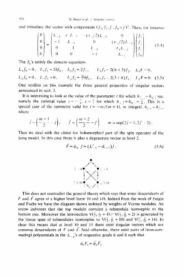
f = < , . , / = ( b ~ , + t L 2)f . (5.6)

z/,.,~ / \ +'+ + 4 0 • ,',, + 2

i)(,,i i',: + 14 • • i~. + 10

l a x / I This does not contradict the general theory which says that some descendents of

F and /~ agree at a higher level (here 10 and 14). Indeed from the work of Feigin and Fuchs we have the diagram shown indexed by weights of Verma modules. An arrow indicates that the top module contains a submodule isomorphic to the bot tom one. Moreover the intersection L L V(~, yg + 4) N V(~, 1 + 2) is generated by

1 I the linear span of submodules isomorphic to V(~2, ~ + 10) and V(~, ~ + 14). In clear this means that at level 10 and 14 there exist singular vectors which are common descendents of F and b ~. Said otherwise, there exist pairs of (non-com- muting) polynomials in the L_~,'s of respective grade 6 and 8 such that

M. Bauer et al. / Singular vectors

is a singular vector at level 10 and similarly

551

¢ " ! -

~bloF 4 = ~012F 2

is singular at level 14. Even in such a simple case the explicit construct ion of these

pairs would be a major undertaking, unless we have a mean to factor (for t = - 3)

the expressions of the opera tors generat ing the corresponding singular vectors at

level 10 and 14, in a non-unique way reflecting the non-commutat ivi ty of the ring. Example 2. Case j '= 1, j = ~ 5 ~t _ ~ , h = - ( 2 t - I + ~ + 4 ).

F = & l , ' f ,

with

q~l, 1/2

and

=L6-1 + A L 4 1 L - 2 + B L ~ I L - 3 + CL2 IL2-2 + DL2-1L-4

+ E L tL 2 L _ 3 + F L _ I L _ 5 + G L 3 2 + I L 2 _ 3 + J L 6 + K L _ 2 L _ 4 ,

8 A = - + 3 t = r t + % +r_~,

t

B _ 8 16

+ 24 - 6 t , t 2 t

16 C = - ~ - + 3 t 2 = r : ' o + r 0 r _ I + r _ l r l ,

24 D - + - - -

t 2

108 72 + 18t ,

t

E _ 32 32 24

+ 24t - 6t 2 , t 3 t 2 t

16 136 264

F t 3 + t 2 t - - + 1 8 4 - 4 8 t + 4 t 2,

16 G = - - - 8 t + t 3 = % + r o + r _ : ,

t

16 16 36 12 + - - + 2 0 - 1 2 t + 2 t 2, t 4 t 3 t 2 t

80 272 316 J t3 t ~ - + - - - 2 0 4 + 7 6 t - 1 2 t 2,

f

(5.7)

32 80 24 K - t 3 + ~5- + - - 2 0 - 2 4 t + 1 0 t 2. (5.8)

t

552 M. Bcttter et ttl. / ~S'mgzdar t'~'ctors

For comparison with the general properties we have introduced the parameters

= )2 ~'M'.M 4(0 IM' + OM , (5.9)

with

~-~=~-~, = t + 4 + 4 t - t ,: , ~ ' o = ~ ' o , = t ~" i = ~ " i , , = t - 4 + 4 t J ( 5 . 1 0 ) ' 2 "

It is not totally obvious how to cast the above expression into a matrix form. This justifies the present endeavour to use fusion as a device to obtain these matrix forms.

Let us look at the implications in the fusion process when V(c, h 0) or V(c, h 1) or both possess singular vectors. Suppose we started by "fusing" fo(xo) and f1(xj) and assume that qbofo(x o) is again a primary field of weight h 0 + n 0. Starting from (f<o~ = f )

1 f,,(xo)f,(x,)--, z,,.+,,._,, E z ' f ~'' ,

r

where the arrow denotes the fusion map of (4.7), we would derive

( (ho f,,) (xo) f , ( x, ) 1

Zho+h~ h+nq~ Y'~Z"~ (') ' r

with a leading term given by

/ ( 1[ d ] ) , ) ~b ('')= ( - 1 ) " " z h°+'' "+""~b 0 L k - - * ~ h , ( k - 1 ) - z ~ - - z Z,,,,+3,,-h f ,

independent of the choice of the coordinate x (be it (x 0 + x~)/2 or x~. . . ). In sect. 3 we considered the representation of the Witt algebra

'{ d 1 I k = - - Z - # A ( k - 1 ) + Z ~ z (5.11)

acting on the basis z P-u and described the effect of substituting l k for L_k in '/'i;,.j, - ~b0 so that with the notations of this section

ttq~ O ( ° ' = ( - 1 ) q~j;,.j,,(,~,/x)f , ~ = - h , , t x = h o + h , - h . (5.12)

Consequently we obtain the following general result:

P r o p o s i t i o n 5 . 1 . If ~i;,,/,, (A = - h i , /~ = h o + h j - h ) = O,

(i) the irreducible module M(c, h) does not occur in the fusion of M(c, h o + n o) ® M(c, h i);

(ii) and as the first non-vanishing term ~0 u), r > O, has to be a highest weight vector, it is necessarily a non-trivial singular vector in V( c, h ).

M. Bauer et al. / Singular vectors 553

A similar property holds of course with the roles of 0 and 1 interchanged.

Let us see how this works in particular interesting cases. i 3 - l h ho, / - j - t j ( j + l ) . Then for A = Case (a). Set h 0 -~h~ ,o - 2 ~t , = =

- h l, I.t = ho + h i - h

q~,o(A /x)=/.~ # + 1 +

quadratic in h I , vanishes for

3 1 h ~ - h . j 4t 2 2 j - j ( j + l ) t , (5.13)

with a Verma module degenerate at level 2(2j + 1) but also for

1 1 h, = -~ + 4 t - J ( J + 1) t , (5.14)

which, using the general formula for singular vectors, one could interpret as h ~./ (sic!) i.e. for generic t it is not the highest weight of a module with a singular vector. Let us choose this second value and look at the fusion symbolically written a s

, / ) , , (½,o) ®"( -~ , -~ (o,j). We have

1 ¢b~. o =L2_, + t L _ 2 . (5.15)

Taking for convenience the fusion point x ~Xl, we get from sect. 4

~-(L_I ~ l) =a~,

h I 1 o~ .~-(L_2® 1) = z2 za~ + ~ z*-2L_k .

k = l (5.16)

Transferring 4,k0 on the h-module and requiring that M(c, h0; x 0) be irreducible we find that

( l(h 1 1 02 + t - ~ - z 0~ + E z * - 2 L - , Zh~,+h,-h E z P f (p) = 0, (5.17)

k = 1 p>~O

which gives a recursive mean to compute the sequence ftP). Now h 0 + h I - h = I - - 1 j - ~t . Therefore the above reads

1 p ( ( 2 j + 1) - p ) f ( P ) = - Y'~ L _ k f (p-k) . (5.18)

t k~>l

554 ;XL Bauer et al. / .S'ingular rector,~

Of course one verifies that for p = 0 this is an identity and that .]~t,~ computed

from this relation agrees with the value obtained from conditions (4.56a, b) of sect. 4 implementing covariance. The main importance of this exercise is to clarify the form we obtained for the singular vectors in thc (0, j) module starting from the second-order equation

/ /( 1 l TI-~(z) ,h,,+h,-t, Y" Z 0; + ~ z 2 ( h ~ - z O : ) + = 0 , (5.19)

- p~I)

where

T ( - ) ( z ) = E z k - 2 L - k (5.20) k ~ l

is the part of the ene rgy-momen tum tensor less singular than z - 2 expressing that

the h o -h~/2 , o Verma module is degenerate at level 2. Indeed the above recursion relation is nothing other than our previous matrix equation for the singular vector, giving a precise meaning to the intermediate stages if we relabel and rescale the components according to

f~i+ M, _ t- i-MfM ' f - i -- f '

using a representation where the generators of angular momentum read (with J0 unchanged, n = j + 1)

0 l ( n - 1) 0

2(n - 2) J

(n - 1)1 0

'0 1 0 1

J + ~ (5.21)

Then f_j+~ . . . . . fi are determined from the recursion relation and the condition

M. Bauer et al. / Singular cectors 555

fj+ 1 _f<2/+ ~)= 0 gives an operator const. × qbo, jf_ / = 0 (with a non-vanishing con- stant factor). Moreover the "descent" equations found among the components fM agree with those derived from the covariance equations.

With this re-interpretation of the singular vectors of type (O,j) we have com- pletely fulfilled the expectations of the advocates of Liouville theory [18]. Of course with obvious changes we obtain the same for the singular vectors of type

(j, 0). Case (b). We set ho-h~,i , hl=-h/,o and h - h i , j , so ~ = h o + h l - h = 2 j j '

and A = - h i =j '(1 + (j ' + 1)/t). In the general expression

2 q~0,/= l-'I { [ I z + ( j + m ) ( l + t ( j + l - m ) ) ] - j<~M~j

× [ I . t + ( j - M ) ( l + t ( j + l + M ) ) ] - 4 A t M 2} (5.22)

the factor corresponding to M = j vanishes, and this is of course expected since V(c, h) is degenerate at level (2j + 1)(2j' + 1) but now we have to implement two distinct conditions, namely (C~o./fo)fl = 0 and f0(~b/.0fl)=0. This is a rather ineffective manner to obtain the singular vector hi, j that we proposed in ref. [12] and that we will illustrate below.

For the same values of h o =-ho. j and h - h/ . j we have also the possibility to choose h~ ---h/,2/ as the second value for which the leading factor (M = j ) in ~b0, j above vanishes. This shows that we have several choices to obtain the ( j ' , j ) singular vector by fusion beyond the "natural" one (0, j ) ® (j ' , 0)--+ (j', j).

Case (c). Inspired by case (a) we finally investigate the more promising fusion

where

] • , ~

( j ' + ½,0) ® " ( - 7,y) --+(j ' , j) ,

,[ ] j ' + 1 +~- h 0 = - ( j ' + ~ 1+ - , (5.23)

" t

and we have used the same abusive notation for

1 1 h, = 4t + 2 - t j ( j + 1), (5.24)

which again for generic t corresponds to an irreducible Verma module, while

h =- - [ tj(j + l) +j +j' + 2jj' + j ' ( j ' + l) " (5.25)

The singular vector operator is d~o- 4'/+ _,',0 and applying proposition 5.1 we

556 M. Bauer el al. / Singular cector~

compute

/I j'+ i i + q~ + ~.,,=- I-I Ix + ( J' + 7 + M' -j'-~-<M'<~]'+~ t

j ' + ~ 4~.M '2 I x t x + ( j ' + ~ - M ' 1+ . (5.26) - t t

I The factor corresponding to M' = j ' + v is /z[/x + (2j ' + 1)(1 + t-J)] - At-~(2j' + 1) 2 . Inserting the values

(1) t x = h o + h ~ - h = ( 2 j ' + 1) j - - ~ ,

p ~ + ( 2 j ' + l ) 1+ = ( 2 j ' + l ) j + l + ,

A ( 2 j ' + I ) 2 2hj ( 1 1 ) t - ( 2 j ' + l ) t = ( 2 j ' + 1 ) 2 - ~ + - ~ - - j ( j + l ) , (5.27)

we do indeed find that this factor vanishes. Consequently we obtain the singular vector in the module V(c, h) by requiring that ~b0f 0 x f l vanishes. It is once again simpler to take the fusion point at x~. We have all data necessary since we know

q5 o -= cb/+ ,~,

~ ( L _ , @ 1) =O z,

9 - ( L p @ l ) ( - 1 ) P [ h , ( p _ l ) + z ( L _Oz)]+k~__oz k k + p - 2 z p _ k L - P - k "

(5.28)

Very much as in case (a) this defines in the V(c, h) module a set of intermediate stages between f = f~o) and f~"), the singular vector set equal to zero in M(c, h). It is readily seen that ( - 1)2~'q~/+ ~.0 (h = - h t, tz = ho + hi - h - n) is the coefficient of f~") at level n in the recursion relation obtained from setting ~bof 0 ×f t - - -0 . This vanishes again since indeed under /x ---)/z - (2j + 1)(2j' + 1) the above values get interchanged as p. <--) - ( g + 2j ' + 1)(1 + t -c) in (5.27) and this is responsible for the fact that at this level we get directly the singular vector (for a generic value

of c).

M. Bauer et aL / Singular cectors 557

(5, 5) singular vector. We need the Let us first show how this reproduces the i

operator

2 4 61,o =-L3 1 + t ( L - I L - 2 + L - 2 L - ' ) + -f2L-3' (5.29)

1 - I I 3 with h~ = ~t + 7 - z t. The substitution

L_l ---~ Oz ,

h I 1 L_2-~ ~ - zOz + ~ z*-2L-,,

k=l

yields

- 2 h I 1 z20Z k=l

L 3 ~ + - + ~ . ~ z k - 3 ( k - 2 ) L _ , , (5.30)

( 4 ( 1 1 2 ) - - Z p - 2L _pO z 03+ 7 h l ' ~ Oz Z Oz + E

p>~l

4)(2h 1 )) z20z p>~l k>~O + 7 + 7 ~ + - + E z"-3(P-2)L- . E z*-'+'-~'*'=o.

(5.31)

This is recast in the recursion relation

0 = k ( k - 4 ) ( k - 2 - t - ' ) f ~*)

+ 2 / - ' Y'~ [ 2 ( k - l - p + t - ' ) + ( p - 2 ) ( l + 2 t - l ) ] L _ p f 'k-v). p>~l

(5.32)

We see indeed that for k = 0 we have an identity while the condition for k = 4 will give the singular vector. Solving recursively

2 fo) = L i f ' l + t

1 2 + - t - -2If, f (2)= [ .i..~_ L _ 1 (l I)L

f(3)= ~ 3 ( t 2_ 1) L ~ l + ( 1 - t - l ) L - I L - 2 + --t(t+l) L - 2 L - j + t - 1 L-3 f '

(5.33)

558 .ll. Batter vtal. / Smgtdar teclor.s

and the fourth equation becomes

O = 3 L i ) " c ~ l + 2 ( l + t I )L J ~ 2 } + ( 4 t

2 --- 4'!, I f , t 2 _ l

I + 1)L 3 , [ ' l l l+6 t tL ~,["

(5.34)

where

qS~ , = L 4 + ( t - t I )2L2 ~ - ..~ - t . ~ + ( t - t - l ) ( L e_ 1L - _ ) + L -_~ L L , ) + 4t IL - l L -_~L 1

( 4 - t ) ( t + 1) (4 + t ) ( t - 1) + L I L _ 3 +

t t L 3L 1 + 3 ( t - t t ) L 4

= L 4 + ( t t ~ 2 _, - ) L L 2 + 3(1 + t) 2 3(1 - t) 2

L2 I L -2 + L 2L21 2t 2t

- ( t + t - l ) L I L 2 L t (5.35)

which agrees with the expression given at the beginning of this section where we used the notation "r+=t ~ + t + + 2 = ( l + _ t ) 2 / t . The intermediate states f--- f(m, f(i), f~2), f(3t satisfy descent equations as did those we wrote at the beginning but do not coincide with those obtained there since our method does not treat t and t ~ symmetrically. Rather by rescaling

2 f ~f(O) = / ( 0 ) f ( l , = f ( l )

l + t

1 2 f(2) = - , f(3) (5.36)

1 + t f(2) 3(t 2 - 1) f ° ) '

we obtain in the tilde basis

E l

0 0

0

=

L_] ( t - t - l ) L _ 2 t 2 ( 4 + t ) ( t - 1 ) L _ 3

- 1 L _ 1 4 t - l L _ 2

0 - 1 L I

0 0 - 1

3(t - t - I ) L _ 4

t - 2 ( 4 - t ) ( t + l ) L _ 3

( t - t - I ) L 2

L_]

f(2)} .

f~l)j f(o) /

(5.37)

M. Bauer et al. / Singular uectors 559

This calculation as we see is straightforward and leads directly to the ( j ' , j ) singular vector. Let us contrast it with the one resulting from the fusion (0, j) ® ( j , 0) ~ (j ' , j ) using again (0, ½) ® (½, 0) ---, ~ • ' (~, ~) as an example. Returning to the

symmetric fusion point x = ( x o + x j )~2, z = xo - x i, let & = 49o, • = L 2_ i + tL 2,

&, =-ch, o=L2_ I + t - l L _ 2 and write

1 E ~V 'k ' (x ) • k ' ( x " ) f ' ( x ' ) ~ z - ~ k>~,,

From ~ofo = 0 and ~blf I = 0 we get respectively for k >/0

3 3 I 2 f ( k - 2 ) 0 = [(~, - ~)(t , - ~ ) - (~ + k t ) ] / ' k ' + (~ - ~ + " t ) L _ , i '~-'' + ~L_,

1 + t E 2,--~y-2L-qftk-u' , (5.38a)

q>~O

1 2 i f ( k - 2 ) - s_ . f ( k - t) + ~ L _ O=[(k-3)(k-1)-(¼+kt-')]f 'k' (k - 3 + { t - ' ) L ,

+ t - ' E ( - 1 ) " q>~O 2q-2 L - q f ( k - q ) " (5.38b)

For k = 0 these two equations become identities as follows from the general discussion. We find that they agree for k = 1, 2, 3 yielding

t - 1 f t l ) _ _ L _ l f '

2(t + 1)

I f(2) = (~L2 1 + . f L _ 2 ) f '

1 (t2+6t+lL3 ) fo ) 3 ( t i _ l ) 16 - ' + ( 3 t 2 + 2 t + 3 ) L - I L - 2 + t L - 3 f ' (5.39)

which can be compared with the values predicted in sect. 4 for the coefficients in the short-distance expansion. Now comes the equation for the singular vector in the module h I. k. Indeed when k = 4 the equations read

0 = 4 ( 2 - t ) f ~4 )+A( t ) f ,

0 = 4 ( 2 - t - l ) f ~ 4 ) + A ( t - I ) f . (5.40)

56O

where

M. Bauer et al. / Singular cectorg

1 [ 5+t ] - I A(t) ~-~ 3 ( t 2 - - 1 ) ( t 2 + 6 t + l ) + l L 4

l [ (5 + t)(3t2 + 2t + 3) 1 + ~ 3 ( t 2 _ 1 ) + l + t L2 IL 2

t t t - - L I L 3 + + L 4 (5.41) 3 ( t + 1 ) 2 L~2 t + 1 - "

Each equation separately involves the unknown contribution f(4) j , so it is insuffi- cient to determine the singular vector. However, they should agree, so that the combination

{ ( 2 - t ' ) A ( t ) - ( 2 - t ) A ( t ' ) } f

is proportional to the singular vector (set equal to zero in M(c, h)). Normalizing to unity the coefficient of L 4 ~ we conclude that

1 ~bL,- t - t - l [ ( 2 - t - I ) A ( t ) - ( 2 - t ) A ( t - ' ) ] , (5.42)

which equals the expression (5.2) as a little algebra readily shows. This mechanism is general. In the fusion of (0, j ) ® (j ' , 0) one verifies that in the

(j',j) module the coefficients f(k~, 0 < k < (2j + 1)(2j' + 1) are determined recur- sively by the conditions th0f0 = 0 or thlfl = 0 and that they agree. On the other hand, at level n = (2j + 1)(2j' + 1) one finds

with

O=aJ(")+Af , O=bnf(")+Bf, (5.43)

a n =D( j , j ' , n , t ) , b~ =D( j ' , j , n , t - ' ) ,

D( j , j ' , k , t ) = J

FI M = - j

[ ( j - M ) ( 2 j ' + l + t ( j + M + l ) ) - k ] , (5.44)

so that up to normalization

~b/,j = const. × (b,A - a,B). (5.45)

While this treatment is symmetric in j and j ' it does not yield a matrix formulation for the singular vectors.

1 Hence we conclude that, among many possibilities, the fusions ( j ' + ~,0)®

"( - ½, j ) " ~ (j ' , j ) or equivalently (0, j + ½) ® "( j ' , - !~ . . . . .) 2- ~ ( J , J directly yield an

M. Bauer et al. / Singular vectors 561

expression for a singular vector. We choose the former to summarize the main

result of this paper.

Proposition 5.2. (i) Verma modules with singular vectors have highest weights parametrized by a

pair ( j ' , j ) with j, j ' non-negative integers or half-integers (eq. (3.6) with 02= t).

When j or j ' vanishes the singular vector is given by the Benoit-Saint-Aubin formula

(3.20), F = c~o. J or F = qb/,of. (ii) I f none o f j and j' vanishes, let f = f ~°> be the highest weight state in V(c ,h) ,

set h o - h / + ~,o, hj - h_ !,~, h - h / , j and

~ z______F_[h , (p_ l )+z (L_ l_O~] + zk k + p - 2 k ~o k

then the equation

1

,~zh,,+h,_ h ~z*f~*~ = o k

determines recursively f t*) for 0 < k < n = (2 j + 1)(2j' + 1) in terms o f f and yields at level n

4~/,J= 0

up to a non-vanishing factor. Moreover the intermediate coefficients ftk), 0 ~< k ~< n satisfy "descent equations" given in (4.56a, b).

To give a last non-trivial example, we recast, using this method, the (1,½) singular vector in the following unnormal ized matrix form:

( ~ l , ½ f ( 0 ) ' 0 . . . . , O) T = A ( f ( 5 ) . . . . . f ( 0 ) ) T '

where the matrix A reads:

(5.46)

- 5 - 2 t - 4 - 4 t - 3 - 6 t - 2 - 8 t - 1 -10 t ~ - 3 L - I t 3 L-2 t---------~ L-3 - - L - 4 - - L - 5 - - L - 6

- " t - 3 t - 3 t - 3 - 1 - 3 - 2 t - 2 - 4 t - 1 - 6 t - 8 t + 1 2--7- 5(t _ - ~ L _ , 5(t - 2---~ L 2 5(t - 2--~ L -3 5(t - 2- - - - -S L-4 5(t - 2-~ L -5

- 1 - 1 - 2 t - 4 t + l - 6 t + 2 0 2t 8 ( t - 1"-----"~ L - I S ( t - i') L-2 8(t - 1 - " " ' ~ L-3 8(t - 1"----"~ L-4

- 1 1 - 2 t + 2 - 4 t + 3 0 0 2t ~ -L_ I 9-----7---- L - 2 9 ~ L -3

- 1 3 - 2 t + 4 0 0 0

2t 8(t + 1- - -" -~ L - I 8(t + 1 - - - " ~ L-2

- 1 5 0 0 0 0

2t 5 ( /+2) L - 1

562 :'~L Bauer et aL / Sin,~uhtr : ectcn:~

W e c o n c l u d e by r e m a r k i n g that the key c o n c e p t is fusion. It a l lows us to t r ans f e r

e q u a t i o n s for s ingu la r vec to r s in a r e d u c i b l e m o d u l e V~ to a m o d u l e V, the best

c h o i c e b e i n g by t e n s o r i n g V~ by an a p p r o p r i a t e o n e c h o s e n to be (gener ica l ly ) an

i r r e d u c i b l e V e r m a m o d u l e . T h e possibi l i ty is d i c t a t e d by the v a n i s h i n g of the

c lass ical q u a n t i t y ~ ( - h ~ , h 0 + h ~ - h), the exp re s s ion o f which plays a c ruc ia l role

in t he d iscuss ion .

References

[1] v. Kac, Leer. Notes in Math. 94 11979) 441 [2] B.L. Feigin and D.B. Fuchs, Funct. Anal. and Appl. 17 119821 114 [Funk. Anal. Priloz. 16, no. 2

(1982) 47] [3] A. Belavin, A. Polyakov and A. Zamolodchikov, Nucl. Phys. B241 (19831 333 [4] C.B. Thorn, Nucl. Phys. B248 (19841 551 [5] V.G. Kac and A.K. Raina, Highest weight representations of infinite dimensional Lie algebras

(World Scientific, Singapore, 19871 [6] D.B. Fuchs, Funct. Anal. and Appl. 23 119891 154 [Funk. Anal. Priloz. 23. no. 2 11989) 81] [7] G. Felder, Nucl. Phys. B317 119891 215 [Erratum B324 (1989) 548] [8] L. Benoit and Y. Saint-Aubin, Phys. Lett. B215 (1988) 517 [9] V.G. Drinfeld and V.V. Sokolov, Journ. Soy. Math. 311 119851 1975

[10] Ph. Di Francesco, C. ltzykson and J.-B. Zuber, Classical W-algebras, Saclay preprint SPhT/911-I49, to be published in Commun. Math. Phys.: C. ltzykson, W-geometry, to appear in Procs. 1990 Carg~se Workshop, and further references therein

[11] J. Balog, L. Feher, L. O'Raifeartaigh, P. ForgAcs and A. Wipf, Phys. Lett. B244 (1990) 435; Ann. Phys. 203 119901 194; L. Bonora and C.S. Xiong, Covariant sl 2 decomposition of the sl, Drinfeld-Sokolov equations and W, algebras, preprint SISSA/ISAS-187/90/EP

[12] M. Bauer, Ph. Di Francesco, C. Itzykson and J.-B. Zuber, Phys. Lett. B260 119911 323 [13] S. Janson and J. Peetre, Math. Nachr. 132 11987) 313 [14] P. Gordan, Invariantentheorie (Teubner, Leipzig, 18871 [15] H. Cohen, Math. Ann. 217 119751 27t [16] B.L. Feigin and D.B. Fuchs, Lect. Notes in Math. 1060 (19841 231) [17] A.V. Lutsyuk, Funct. Anal. and Appl. 8 (19741 351 [Funk. Anal. Priloz. 8, no. 4 119741 91] [18] J.-L. Gervais and A. Neveu, Nucl. Phys. B264 (19861 557 [19] G. Segal, The definition of conformal field theory, in Links between geometry and physics, MP1

87-58; G. Moore and N. Seiberg, Lectures on RCFT, lectures at the 1989 Trieste Spring School

[20] R. Brustein, S. Yankielowicz and J.-B. Zuber, Nucl. Phys. B313 (1989) 321