serdar kucuk kinematics, singularity and dexterity...
TRANSCRIPT

Kinematics, Singularity and Dexterity Analysis of Planar Parallel Manipulators Based on DH Method 387
Kinematics, Singularity and Dexterity Analysis of Planar Parallel Manipulators Based on DH Method
Serdar Kucuk
x
Kinematics, Singularity and Dexterity Analysis of Planar Parallel
Manipulators Based on DH Method
Serdar Kucuk Kocaeli University
Turkey
1. Introduction
Parallel manipulators have separate serial kinematic chains that are linked to the ground and the moving platform at the same time. They have some potential advantages over serial robot manipulators such as high accuracy, greater load capacity, high mechanical rigidity, high velocity and acceleration (Kang et al., 2001; Kang & Mills, 2001). Planar Parallel Manipulators (PPMs), performing two translations along the x and y axes, and rotation through an angle of around the z axis are a special group among the parallel robot manipulators. They have potential advantages for microminiaturization (Hubbard et al., 2001) and pick-and-place operations (Heerah et al., 2003). However, due to the complexity of the closed-loop chain mechanism, the kinematics analysis of parallel manipulators is more difficult than their serial counterparts. Therefore selection of an efficient mathematical model is very important for simplifying the complexity of the kinematics problems in parallel robots. In this book chapter, the forward and inverse kinematics problems of PPMs are solved based on D-H method (Denavit & Hartenberg, 1955) which is a common kinematic modelling convention using 4x4 homogenous transformation matrices. The easy physical interpretation of the robot mechanisms is the main advantage of this method. The Forward kinematics problem calculates the position and orientation of the end-effector if the set of joint angles are known. The inverse kinematics problem solves for the joint angles when the position and orientation of the end effector is given. In contrast to serial manipulators, the forward kinematics problem is much more difficult than the inverse kinematic problem for parallel manipulators. Afterwards very practical definitions are provided for Jacobian matrix and workspace determination of PPMs which are required for singularity and dexterity analyses. Rest of this book chapter is composed of the following sections. Some fundamental definitions about D-H method as a kinematics modelling convention, Jacobian matrix, condition number, global dexterity index, singularity and workspace determination are presented in Section 2. A two-degree-of-freedom (2-dof) PPM and a 3-dof Fully Planar Parallel Manipulator (FPPM) are given as examples to illustrate the methodology in the following Section. FPPMs are composed of a moving platform linked to
21
www.intechopen.com

Robot Manipulators, New Achievements388
the ground by three independent limbs including one active (actuated) joint in each (Merlet, 1996). The conclusions with final remarks are presented in the last section.
2. Background
2.1 Denavit-Hartenberg convention The D-H convention (Denavit & Hartenberg, 1955) based on 4x4 homogenous transformation matrices is commonly used kinematic modelling convention for the robotics community. The easy physical interpretation of the robot mechanisms is the main advantage of this method. A spatial transformation between two consecutive links can be described by a set of parameters, namely ,1j 1ja , j and jd . Using these parameters, the general
form of the transformation matrix for adjacent coordinate frames, j-1 and j is obtained as
1000dcoscossincossinsindsinsincoscoscossin
a0sincos
Tj1j1j1jj1jj
j1j1j1jj1jj
1jjj
1jj (1)
The transformation of the link n coordinate frame into the base coordinate frame of the robot manipulator is given by
TTTTT 1nn
1j2j
j1j
1jj
1jn
(2)
where j=1, 2, 3, ..., n. 2.2 Jacobian Matrix, Condition Number and Global Dexterity Index Dexterity is an essential topic for design and conceptual control of robotic manipulators. It can be described as the ability to perform infinitesimal movement in the arbitrary directions as easily as possible in the workspace of the robotic manipulators. It is based on the condition number () of the manipulator Jacobian matrix (Gosselin & Angeles, 1991).
1JJ (3)
where J illustrates the Jacobian matrix and denotes the Frobenius norm of the matrix. varies between 1 to . In general, =1/ is used for limiting the dexterity between 0 and 1. Thus dexterity of a manipulator can be easily measured. It is well known that as =1 represents a perfect isotropic dexterity, =0 illustrates singular configuration. Then the kinematic relations for the planar parallel manipulators can be expressed as
f(x,q)=0 (4)
where f is the function of x ),y,x( T and q=(q1, q2, and qn) T, and 0 is n dimensional zero vector. The parameters x, y and are the position and orientation of the end-effector in terms of base frame. Additionally, q1, q2 and qn represent the actuated joint variables. The following term is obtained differentiating the equation 4 with respect to the time.
Ax+Bq=0 (5) where x and q are the time derivatives of x and q, respectively. A and B are two separate Jacobian matrices. The overall Jacobian matrix for a parallel manipulator can be obtained as
ABJ 1 (6) Since the dexterity demonstrates the local property of a mechanism, designers requires a global one. Gosselin and Angeles (1991) introduced Global Dexterity Index (GDI) in order to measure the global property of the manipulators. GDI defined as
BAGDI (7)
where B represents the area of the workspace and A is
xy
dxdyd1A (8)
2.3 Singularity Three types of singularities exist for planar parallel manipulators (Tsai, 1999; Merlet, 2000). They occur when either determinant of the matrices A or B or both are zero. When the determinant of A and B goes to zero, the direct and inverse kinematics singularities occur, respectively. Direct kinematics singularity occurs inside the workspace of the manipulator. Inverse kinematics singularity occurs at the boundaries of the manipulator’s workspace where any limb is completely stretched-out or folded-back.
2.4 Workspace Determination Workspace determination is a very significant step in analyzing robot manipulators. Its determination is necessary for conceptual design and trajectory planning. Many researches (Agrawal, 1990; Gosselin, 1990; Merlet, 1995; Merlet et al., 1998) focused on the workspace determination of parallel manipulators. Merlet, Gosselin and Mouly (1998) outlined some workspace definitions for PPMs such as constant orientation workspace, reachable workspace and dexterous workspace. The constant orientation workspace (considered also in this book chapter) is the area that can be reached by the end-effector with constant orientation. In general, geometrical (Bonev & Ryu, 2001; Gosselin & Guillot, 1991) and numerical methods (Kim et al., 1997) are used for workspace determination of parallel manipulators. Computation of workspace based on geometrical method is difficult and may not be obtained due to the complexity of the closed-loop chain mechanisms (Fichter, 1986).
. .
. .
www.intechopen.com

Kinematics, Singularity and Dexterity Analysis of Planar Parallel Manipulators Based on DH Method 389
the ground by three independent limbs including one active (actuated) joint in each (Merlet, 1996). The conclusions with final remarks are presented in the last section.
2. Background
2.1 Denavit-Hartenberg convention The D-H convention (Denavit & Hartenberg, 1955) based on 4x4 homogenous transformation matrices is commonly used kinematic modelling convention for the robotics community. The easy physical interpretation of the robot mechanisms is the main advantage of this method. A spatial transformation between two consecutive links can be described by a set of parameters, namely ,1j 1ja , j and jd . Using these parameters, the general
form of the transformation matrix for adjacent coordinate frames, j-1 and j is obtained as
1000dcoscossincossinsindsinsincoscoscossin
a0sincos
Tj1j1j1jj1jj
j1j1j1jj1jj
1jjj
1jj (1)
The transformation of the link n coordinate frame into the base coordinate frame of the robot manipulator is given by
TTTTT 1nn
1j2j
j1j
1jj
1jn
(2)
where j=1, 2, 3, ..., n. 2.2 Jacobian Matrix, Condition Number and Global Dexterity Index Dexterity is an essential topic for design and conceptual control of robotic manipulators. It can be described as the ability to perform infinitesimal movement in the arbitrary directions as easily as possible in the workspace of the robotic manipulators. It is based on the condition number () of the manipulator Jacobian matrix (Gosselin & Angeles, 1991).
1JJ (3)
where J illustrates the Jacobian matrix and denotes the Frobenius norm of the matrix. varies between 1 to . In general, =1/ is used for limiting the dexterity between 0 and 1. Thus dexterity of a manipulator can be easily measured. It is well known that as =1 represents a perfect isotropic dexterity, =0 illustrates singular configuration. Then the kinematic relations for the planar parallel manipulators can be expressed as
f(x,q)=0 (4)
where f is the function of x ),y,x( T and q=(q1, q2, and qn) T, and 0 is n dimensional zero vector. The parameters x, y and are the position and orientation of the end-effector in terms of base frame. Additionally, q1, q2 and qn represent the actuated joint variables. The following term is obtained differentiating the equation 4 with respect to the time.
Ax+Bq=0 (5) where x and q are the time derivatives of x and q, respectively. A and B are two separate Jacobian matrices. The overall Jacobian matrix for a parallel manipulator can be obtained as
ABJ 1 (6) Since the dexterity demonstrates the local property of a mechanism, designers requires a global one. Gosselin and Angeles (1991) introduced Global Dexterity Index (GDI) in order to measure the global property of the manipulators. GDI defined as
BAGDI (7)
where B represents the area of the workspace and A is
xy
dxdyd1A (8)
2.3 Singularity Three types of singularities exist for planar parallel manipulators (Tsai, 1999; Merlet, 2000). They occur when either determinant of the matrices A or B or both are zero. When the determinant of A and B goes to zero, the direct and inverse kinematics singularities occur, respectively. Direct kinematics singularity occurs inside the workspace of the manipulator. Inverse kinematics singularity occurs at the boundaries of the manipulator’s workspace where any limb is completely stretched-out or folded-back.
2.4 Workspace Determination Workspace determination is a very significant step in analyzing robot manipulators. Its determination is necessary for conceptual design and trajectory planning. Many researches (Agrawal, 1990; Gosselin, 1990; Merlet, 1995; Merlet et al., 1998) focused on the workspace determination of parallel manipulators. Merlet, Gosselin and Mouly (1998) outlined some workspace definitions for PPMs such as constant orientation workspace, reachable workspace and dexterous workspace. The constant orientation workspace (considered also in this book chapter) is the area that can be reached by the end-effector with constant orientation. In general, geometrical (Bonev & Ryu, 2001; Gosselin & Guillot, 1991) and numerical methods (Kim et al., 1997) are used for workspace determination of parallel manipulators. Computation of workspace based on geometrical method is difficult and may not be obtained due to the complexity of the closed-loop chain mechanisms (Fichter, 1986).
. .
. .
www.intechopen.com
Robot Manipulators, New Achievements390
Alternatively, numerical methods based on the discretization of Cartesian space (Kim et al., 1997) in general, are also used in this study due to their simplicity according to the geometrical methods. In discretization method, firstly a Cartesian area is discretized into “PxQ” points along the X and Y axes. Secondly each pose in this discretized Cartesian area is examined whether belonging to the workspace of the manipulator.
3. Examples
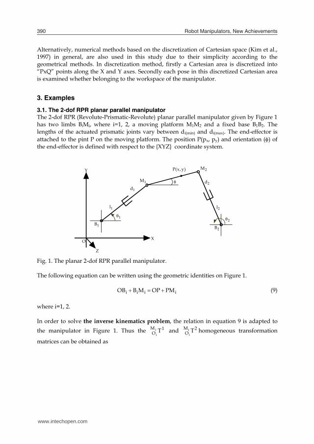
3.1. The 2-dof RPR planar parallel manipulator The 2-dof RPR (Revolute-Prismatic-Revolute) planar parallel manipulator given by Figure 1 has two limbs BiMi, where i=1, 2, a moving platform M1M2 and a fixed base B1B2. The lengths of the actuated prismatic joints vary between di(min) and di(max). The end-effector is attached to the pint P on the moving platform. The position P(px, py) and orientation () of the end-effector is defined with respect to the {XYZ} coordinate system.
Z
X
Y
1l
2M
1M
1B
)y,x(P
1d
1
O
2l
2d
2B2
Fig. 1. The planar 2-dof RPR parallel manipulator. The following equation can be written using the geometric identities on Figure 1.
iiii PMOPMBOB (9) where i=1, 2. In order to solve the inverse kinematics problem, the relation in equation 9 is adapted to the manipulator in Figure 1. Thus the 1M
O Tii
and 2MO Ti
ihomogeneous transformation
matrices can be obtained as
10000010
dl1000001
1000010000cossin00sincos
10000100
OB010OB001
T iiii
ii
y
x
1MO
i
i
ii
10000010
)ld(cosOBcos0sin)ld(sinOBsin0cos
iiiyii
iiixii
i
i
(10)
100001000010
PM001
1000010000cossin00sincos
10000100
p010p001
T
i
ii
ii
y
x
2MO
ii
10000100
sinPMp0cossincosPMp0sincos
iiy
iix
(11)
where 1 and 2 . Since the position vectors of 1MO Ti
iand 2M
O Tii
matrices are
equal, one can write the following equations easily.
i
i
yiiy
xiix
iii
iiiOBsinPMpOBcosPMp
)ld(cos)ld(sin
(12)
Summing the squares of the both sides in the equation 12, we obtain, after simplification,
iiii yyxx2y
2x
2y
2x
2ii OBp2OBp2OBOBppPMQ
0)ld()OBp(PMsin2)OBp(PMcos2 2iiyyiixxii ii
(13)
The active joint variables di can be found using equation 13 as follows.
iyyiixxii
yyxx2y
2x
2y
2x
2i
i l)OBp(PMsin2)OBp(PMcos2
OBp2OBp2OBOBppPMd
ii
ii11 (14)
Once the active joint variables d1 and d2 are solved, the passive joint variable θ1 and θ2 can be found from the equation 12 by back substitution.
www.intechopen.com
Kinematics, Singularity and Dexterity Analysis of Planar Parallel Manipulators Based on DH Method 391
Alternatively, numerical methods based on the discretization of Cartesian space (Kim et al., 1997) in general, are also used in this study due to their simplicity according to the geometrical methods. In discretization method, firstly a Cartesian area is discretized into “PxQ” points along the X and Y axes. Secondly each pose in this discretized Cartesian area is examined whether belonging to the workspace of the manipulator.
3. Examples
3.1. The 2-dof RPR planar parallel manipulator The 2-dof RPR (Revolute-Prismatic-Revolute) planar parallel manipulator given by Figure 1 has two limbs BiMi, where i=1, 2, a moving platform M1M2 and a fixed base B1B2. The lengths of the actuated prismatic joints vary between di(min) and di(max). The end-effector is attached to the pint P on the moving platform. The position P(px, py) and orientation () of the end-effector is defined with respect to the {XYZ} coordinate system.
Z
X
Y
1l
2M
1M
1B
)y,x(P
1d
1
O
2l
2d
2B2
Fig. 1. The planar 2-dof RPR parallel manipulator. The following equation can be written using the geometric identities on Figure 1.
iiii PMOPMBOB (9) where i=1, 2. In order to solve the inverse kinematics problem, the relation in equation 9 is adapted to the manipulator in Figure 1. Thus the 1M
O Tii
and 2MO Ti
ihomogeneous transformation
matrices can be obtained as
10000010
dl1000001
1000010000cossin00sincos
10000100
OB010OB001
T iiii
ii
y
x
1MO
i
i
ii
10000010
)ld(cosOBcos0sin)ld(sinOBsin0cos
iiiyii
iiixii
i
i
(10)
100001000010
PM001
1000010000cossin00sincos
10000100
p010p001
T
i
ii
ii
y
x
2MO
ii
10000100
sinPMp0cossincosPMp0sincos
iiy
iix
(11)
where 1 and 2 . Since the position vectors of 1MO Ti
iand 2M
O Tii
matrices are
equal, one can write the following equations easily.
i
i
yiiy
xiix
iii
iiiOBsinPMpOBcosPMp
)ld(cos)ld(sin
(12)
Summing the squares of the both sides in the equation 12, we obtain, after simplification,
iiii yyxx2y
2x
2y
2x
2ii OBp2OBp2OBOBppPMQ
0)ld()OBp(PMsin2)OBp(PMcos2 2iiyyiixxii ii
(13)
The active joint variables di can be found using equation 13 as follows.
iyyiixxii
yyxx2y
2x
2y
2x
2i
i l)OBp(PMsin2)OBp(PMcos2
OBp2OBp2OBOBppPMd
ii
ii11 (14)
Once the active joint variables d1 and d2 are solved, the passive joint variable θ1 and θ2 can be found from the equation 12 by back substitution.
www.intechopen.com

Robot Manipulators, New Achievements392
)ld(
OBsinPMp,
)ld(OBcosPMp
2tanaii
yiiy
ii
xiixi
ii (15)
The Jacobian matrix of the 2-dof RPR is computed using the equation 13 as follows.
0qBxA
0dd
dQ
dQ
dQ
dQ
pp
pQ
pQ
pQ
pQ
2
1
2
2
1
2
2
1
1
1
y
x
y
2
x
2
y
1
x
1
0dd
ld00ld
pp
PMsinOBpPMcosOBpPMsinOBpPMcosOBp
2
1
22
11
y
x
22yy22xx
11yy11xx
22
11
(16)
The overall Jacobian matrix is obtained as
22
22yy
22
22xx
11
11yy
11
11xx
ldPMsinOBp
ldPMcosOBp
ldPMsinOBp
ldPMcosOBp
J22
11
(17)
Numerical example for the inverse kinematics: The dimensions of the planar 2-dof RPR parallel manipulator are given as l1=l2=12, PM1=PM2=3, OBx1=0, OBy1=0, OBx2=15, OBy2=0, px=11, py=20 and =30º. According to the data above, the active joint variables d1 and d2 can be found as 8.3185 and 9.5457, respectively. The passive joint variables θ1 and θ2 are found as -24.4256 and 3.7307, respectively by back substitution. Numerical example for the Jacobian matrix and condition number: Using the dimensions of the inverse kinematics example above, the Jacobian matrix and condition number are found as
0.99790.0651-0.91050.4135
J and 2.1192 (18)
Numerical example for the workspace determination: The dimensions of the manipulator are given as l1=l2=10, PM1=PM2=2, OBx1=0, OBy1=0, OBx2=20 and OBy2=0 and. The lengths of the actuated prismatic joints vary between di(min)=0 and di(max)=7, where i=1,2. The workspace is obtained as 102.3888 for =0º orientation. The limits of the discretized Cartesian area are denoted by the red rectangle shown in Figure 2a. The black and green areas show reachable and non-reachable workspaces of the manipulator, respectively. Numerical example for the dexterity and singularity analysis: The Figure 2b shows the inverse dexterity of the manipulator using the same dimensions given by example for workspace determination. The GDI of the manipulator are found as 0.0012. As seen in Figure 2b, since the inverse of the condition numbers colored with red areas are so close to
the unity, there isn’t any singular point occurred inside reachable workspace. The red and blue areas show reachable and non-reachable workspaces of the manipulator, respectively.
3.2. The 3-dof RPR planar parallel manipulator The 3-dof RPR planar parallel manipulator shown in Figure 3 has three limbs BiMi, where i=1, 2, 3. P denotes the point where the end-effector is located at the moving platform which is chosen as equilateral triangle. The angle represents the orientation of the end-effector. If a line AB passing through the point P is drawn parallel to the M1M2, the angles PM1M2 ( 1 ) and PM2M1 ( 2 ) are equal to the angles APM1 and M2PB, respectively. The angles between the lines BP and PM1, M2P and PB, BP and PM3 are denoted as λ1, λ2 and λ3, respectively.
0
5
10
15
20
-20
-10
0
10
20
0
0.5
1
XY
Fig. 2. a) Workspace, b) dexterity graph, for planar 2-dof RPR parallel manipulator.
3l
Z
X
Y
1l
3M
2M
1M
1B
)y,x(P
1d
1
O
2l
2d
3d
x
y
z
2B
2
3B
3
Fig. 3. The planar 3-dof RPR parallel manipulator.
www.intechopen.com

Kinematics, Singularity and Dexterity Analysis of Planar Parallel Manipulators Based on DH Method 393
)ld(
OBsinPMp,
)ld(OBcosPMp
2tanaii
yiiy
ii
xiixi
ii (15)
The Jacobian matrix of the 2-dof RPR is computed using the equation 13 as follows.
0qBxA
0dd
dQ
dQ
dQ
dQ
pp
pQ
pQ
pQ
pQ
2
1
2
2
1
2
2
1
1
1
y
x
y
2
x
2
y
1
x
1
0dd
ld00ld
pp
PMsinOBpPMcosOBpPMsinOBpPMcosOBp
2
1
22
11
y
x
22yy22xx
11yy11xx
22
11
(16)
The overall Jacobian matrix is obtained as
22
22yy
22
22xx
11
11yy
11
11xx
ldPMsinOBp
ldPMcosOBp
ldPMsinOBp
ldPMcosOBp
J22
11
(17)
Numerical example for the inverse kinematics: The dimensions of the planar 2-dof RPR parallel manipulator are given as l1=l2=12, PM1=PM2=3, OBx1=0, OBy1=0, OBx2=15, OBy2=0, px=11, py=20 and =30º. According to the data above, the active joint variables d1 and d2 can be found as 8.3185 and 9.5457, respectively. The passive joint variables θ1 and θ2 are found as -24.4256 and 3.7307, respectively by back substitution. Numerical example for the Jacobian matrix and condition number: Using the dimensions of the inverse kinematics example above, the Jacobian matrix and condition number are found as
0.99790.0651-0.91050.4135
J and 2.1192 (18)
Numerical example for the workspace determination: The dimensions of the manipulator are given as l1=l2=10, PM1=PM2=2, OBx1=0, OBy1=0, OBx2=20 and OBy2=0 and. The lengths of the actuated prismatic joints vary between di(min)=0 and di(max)=7, where i=1,2. The workspace is obtained as 102.3888 for =0º orientation. The limits of the discretized Cartesian area are denoted by the red rectangle shown in Figure 2a. The black and green areas show reachable and non-reachable workspaces of the manipulator, respectively. Numerical example for the dexterity and singularity analysis: The Figure 2b shows the inverse dexterity of the manipulator using the same dimensions given by example for workspace determination. The GDI of the manipulator are found as 0.0012. As seen in Figure 2b, since the inverse of the condition numbers colored with red areas are so close to
the unity, there isn’t any singular point occurred inside reachable workspace. The red and blue areas show reachable and non-reachable workspaces of the manipulator, respectively.
3.2. The 3-dof RPR planar parallel manipulator The 3-dof RPR planar parallel manipulator shown in Figure 3 has three limbs BiMi, where i=1, 2, 3. P denotes the point where the end-effector is located at the moving platform which is chosen as equilateral triangle. The angle represents the orientation of the end-effector. If a line AB passing through the point P is drawn parallel to the M1M2, the angles PM1M2 ( 1 ) and PM2M1 ( 2 ) are equal to the angles APM1 and M2PB, respectively. The angles between the lines BP and PM1, M2P and PB, BP and PM3 are denoted as λ1, λ2 and λ3, respectively.
0
5
10
15
20
-20
-10
0
10
20
0
0.5
1
XY
Fig. 2. a) Workspace, b) dexterity graph, for planar 2-dof RPR parallel manipulator.
3l
Z
X
Y
1l
3M
2M
1M
1B
)y,x(P
1d
1
O
2l
2d
3d
x
y
z
2B
2
3B
3
Fig. 3. The planar 3-dof RPR parallel manipulator.
www.intechopen.com
Robot Manipulators, New Achievements394
If the relation in equation 9 is adapted to the manipulator in Figure 3, the 1MO Ti
i and
2MO Ti
ihomogeneous transformation matrices can be obtained as
10000010
dl1000001
1000010000cossin00sincos
10000100
OB010OB001
T iiii
ii
y
x
1MO
i
i
ii
10000010
)ld(cosOBcos0sin)ld(sinOBsin0cos
iiiyii
iiixii
i
i
(19)
where i=1, 2, 3.
100001000010
PM001
1000010000)cos()sin(00)sin()cos(
10000100
p010p001
T
i
ii
ii
y
x
2MO
ii
10000100
)sin(PMp0)cos()sin()cos(PMp0)sin()cos(
iiyii
iixii
(20)
where 11 and 22 . Since the position vectors of 1M
O Tii
and 2MO Ti
imatrices are
equal, one can write easily the following equations.
iii
iii
yyxy
xyxx
iii
iiiOBcossinpOBsincosp
)ld(cos)ld(sin
(21)
where iix cosPM
i and iiiy sinPM . Summing the squares of the both sides in the
equation 21, we obtain, after simplification,
iiiiii yyxx2y
2x
2y
2x
2y
2xi OBp2OBp2OBOBppQ
)OBOBpp(cos2iiiiii yyxxyyxx
0)ld()OBOBpp(sin2 2iiyxxyyxxy iiiiii
(22)
The inverse kinematics problem is solved using the equation 22 as follows.
i
yxxyyxxy
yyxxyyxx
yyxx2y
2x
2y
2x
2y
2x
i l
)OBOBpp(sin2
)OBOBpp(cos2
OBp2OBp2OBOBpp
d
iiiiii
iiiiii
iiiiii
(23)
Once the d1, d2 and d3 are obtained, the angles θ1, θ2 and θ3 can be determined from the equation 21 by back substitution.
)ld(
OBcossinp,
)ld(OBsincosp
2tanaii
yyxy
ii
xyxxi
iiiiii (24)
The forward kinematics problem is found rearranging the equation 22 as follows.
0cpbpapp iyixi2y
2x (i=1,2,3) (25)
where )sinOB(cos2a
iii yxxi , )OBsin(cos2biii yxyi and 2
xi iOBc
2iixyyxyyxx
2y
2x
2y )ld()OBOB(sin2)OBOB(cos2OB
iiiiiiiiiii
One can obtain the following new system of equations using equation 25.
0)cc(p)bb(p)aa( 21y21x21 0)cc(p)bb(p)aa( 31y31x31
0)cc(p)bb(p)aa( 32y32x32 (26)
One can write the following equations using the equation 26.
12y12x12 cpbpa 13y13x13 cpbpa (27)
where 2112 aaa , 2112 bbb , 1212 ccc , 3113 aaa , 3113 bbb and
1313 ccc . The px and py can be obtained applying the elimination method to the equation 27 as
)abab(cbcbp
12131312
12131312x
and )baba(
cacap13121213
13121213y
(28)
The orientation angle ( ) can be found using i=3 in equation 25.
www.intechopen.com

Kinematics, Singularity and Dexterity Analysis of Planar Parallel Manipulators Based on DH Method 395
If the relation in equation 9 is adapted to the manipulator in Figure 3, the 1MO Ti
i and
2MO Ti
ihomogeneous transformation matrices can be obtained as
10000010
dl1000001
1000010000cossin00sincos
10000100
OB010OB001
T iiii
ii
y
x
1MO
i
i
ii
10000010
)ld(cosOBcos0sin)ld(sinOBsin0cos
iiiyii
iiixii
i
i
(19)
where i=1, 2, 3.
100001000010
PM001
1000010000)cos()sin(00)sin()cos(
10000100
p010p001
T
i
ii
ii
y
x
2MO
ii
10000100
)sin(PMp0)cos()sin()cos(PMp0)sin()cos(
iiyii
iixii
(20)
where 11 and 22 . Since the position vectors of 1M
O Tii
and 2MO Ti
imatrices are
equal, one can write easily the following equations.
iii
iii
yyxy
xyxx
iii
iiiOBcossinpOBsincosp
)ld(cos)ld(sin
(21)
where iix cosPM
i and iiiy sinPM . Summing the squares of the both sides in the
equation 21, we obtain, after simplification,
iiiiii yyxx2y
2x
2y
2x
2y
2xi OBp2OBp2OBOBppQ
)OBOBpp(cos2iiiiii yyxxyyxx
0)ld()OBOBpp(sin2 2iiyxxyyxxy iiiiii
(22)
The inverse kinematics problem is solved using the equation 22 as follows.
i
yxxyyxxy
yyxxyyxx
yyxx2y
2x
2y
2x
2y
2x
i l
)OBOBpp(sin2
)OBOBpp(cos2
OBp2OBp2OBOBpp
d
iiiiii
iiiiii
iiiiii
(23)
Once the d1, d2 and d3 are obtained, the angles θ1, θ2 and θ3 can be determined from the equation 21 by back substitution.
)ld(
OBcossinp,
)ld(OBsincosp
2tanaii
yyxy
ii
xyxxi
iiiiii (24)
The forward kinematics problem is found rearranging the equation 22 as follows.
0cpbpapp iyixi2y
2x (i=1,2,3) (25)
where )sinOB(cos2a
iii yxxi , )OBsin(cos2biii yxyi and 2
xi iOBc
2iixyyxyyxx
2y
2x
2y )ld()OBOB(sin2)OBOB(cos2OB
iiiiiiiiiii
One can obtain the following new system of equations using equation 25.
0)cc(p)bb(p)aa( 21y21x21 0)cc(p)bb(p)aa( 31y31x31
0)cc(p)bb(p)aa( 32y32x32 (26)
One can write the following equations using the equation 26.
12y12x12 cpbpa 13y13x13 cpbpa (27)
where 2112 aaa , 2112 bbb , 1212 ccc , 3113 aaa , 3113 bbb and
1313 ccc . The px and py can be obtained applying the elimination method to the equation 27 as
)abab(cbcbp
12131312
12131312x
and )baba(
cacap13121213
13121213y
(28)
The orientation angle ( ) can be found using i=3 in equation 25.
www.intechopen.com

Robot Manipulators, New Achievements396
0cpbpapp 3y3x32y
2x (29)
If px and py in equation 28 are substituted in equation 29, one can obtain after simplification
0cba 2333
22 (30) where )abab( 12131312 , 12131312 cbcb and 13121213 caca . The equation 30
can be converted into the eight-degree polynomial using 2t1t2sin and 2
2
t1t1cos
.
The roots of this polynomial are the answer of the forward kinematics problem. Once is determined, px and py can be found easily substituting the angle in equation 28. After having position (px, py) and orientation (), the passive joint angles can be found using the equation 21 by back substitution
)ld(
OBcossinp,
)ld(OBsincosp
2tanAii
yyxy
ii
xyxxi
iiiiii (31)
The Jacobian matrix of the 3-dof PPM shown in Figure 3 is computed as follows.
0
d
d
d
dQ
dQ
dQ
dQ
dQ
dQ
dQ
dQ
dQ
pp
pQ
pQ
pQ
pQ
pQ
pQ
QpQ
pQ
3
2
1
3
3
2
3
1
3
3
2
2
2
1
2
3
1
2
1
1
1
y
x
3
y
3
x
3
2
y
2
x
2
1
y
1
x
1
0ddd
ld000ld000ld
pp
3
2
1
33
22
11
y
x
333
222
111
(32)
where
iii yxxxi sincosOBp (33)
iii xyyyi sincosOBp (34)
)OBOBpp(cos
)OBOBpp(sin
iiiiii
iiiiii
yxxyyxxy
yyxxyyxxi
(35)
The overall Jacobian matrix is obtained as
33
3
33
3
33
3
22
2
22
2
22
2
11
1
11
1
11
1
ldldld
ldldld
ldldld
J (36)
Numerical example for the inverse kinematics: The dimensions of the planar 3-dof RPR parallel manipulator are given as l1=10, l2=10, l3=10, OBx1=0, OBy1=0, OBx2=20, OBy2=0, OBx3=10, OBy3=45, M1M2=15. The position of the point P in terms of the coordinate frame {xyz} attached to the M1 corner of the moving platform is chosen as (4, 5). The angles λ1, λ2 and λ3 are computed as 231.3402, -24.4440 and 66.3453, where 51.34021 and
24.4440,2 respectively. Moreover, the lengths PM1, PM2 and PM3 are determined as 6.4031, 12.0830 and 8.7233, respectively. If the position and orientation in terms of the base frame {XYZ} are given as px=12, py=18 and =30º, the active joint variables d1 d2 and d3 can be found as 6.0617, 9.5881 and 8.3594, respectively. The passive joint variables θ1, θ2 and θ3
are found as -43.4006, -11.8615 and -176.7655, respectively by back substitution. Numerical example for the forward kinematics: The dimensions of manipulator are given as l1=11, l2=11, l3=11, OBx1=0, OBy1=0, OBx2=10, OBy2=0, OBx3=5, OBy3=32, M1M2=10. The position of the point P in terms of the coordinate frame {xyz} is chosen as (5, 2.8868). The angles λ1, λ2 and λ3 are computed as 210.0004, -30.0004 and 90, where 301 and
30.0004,2 respectively. Moreover, the lengths PM1, PM2 and PM3 are determined as 8.4853, 7.8102 and 3.5616, respectively. If the active and passive joint variables are given as d1=8, d2=7.9999, d3=7.9999 and θ1=-52.1046, θ2=-52.105, θ3=-127.8937, the position and orientation of end-effector in terms of base coordinate frame {XYZ} are found as px=19,9936 py=14.5569 and =0.000932º, respectively. Numerical example for the Jacobian matrix and condition number: Using the dimensions of numerical example for the inverse kinematics above, the Jacobian matrix and condition number are found as
0.47340.9984-0.056411.52900.97860.20553.64890.72660.6871
J and 8.1351 (37)
Numerical example for the workspace determination: The dimensions of the manipulator are given as l1=l2=l3=8.5, OBx1=0, OBy1=0, OBx2=17, OBy2=0, OBx3=9, OBy3=40, M1M2=16. The lengths of the actuated prismatic joints vary between di(min)=0 and di(max)=8.5, where i=1,2,3. If the position of the point P in terms of the coordinate frame {xyz} is chosen as (7, 7), the angles λ1, λ2 and λ3 are computed as 225, -37.8750 and 81.7020, where 541 and
www.intechopen.com

Kinematics, Singularity and Dexterity Analysis of Planar Parallel Manipulators Based on DH Method 397
0cpbpapp 3y3x32y
2x (29)
If px and py in equation 28 are substituted in equation 29, one can obtain after simplification
0cba 2333
22 (30) where )abab( 12131312 , 12131312 cbcb and 13121213 caca . The equation 30
can be converted into the eight-degree polynomial using 2t1t2sin and 2
2
t1t1cos
.
The roots of this polynomial are the answer of the forward kinematics problem. Once is determined, px and py can be found easily substituting the angle in equation 28. After having position (px, py) and orientation (), the passive joint angles can be found using the equation 21 by back substitution
)ld(
OBcossinp,
)ld(OBsincosp
2tanAii
yyxy
ii
xyxxi
iiiiii (31)
The Jacobian matrix of the 3-dof PPM shown in Figure 3 is computed as follows.
0
d
d
d
dQ
dQ
dQ
dQ
dQ
dQ
dQ
dQ
dQ
pp
pQ
pQ
pQ
pQ
pQ
pQ
QpQ
pQ
3
2
1
3
3
2
3
1
3
3
2
2
2
1
2
3
1
2
1
1
1
y
x
3
y
3
x
3
2
y
2
x
2
1
y
1
x
1
0ddd
ld000ld000ld
pp
3
2
1
33
22
11
y
x
333
222
111
(32)
where
iii yxxxi sincosOBp (33)
iii xyyyi sincosOBp (34)
)OBOBpp(cos
)OBOBpp(sin
iiiiii
iiiiii
yxxyyxxy
yyxxyyxxi
(35)
The overall Jacobian matrix is obtained as
33
3
33
3
33
3
22
2
22
2
22
2
11
1
11
1
11
1
ldldld
ldldld
ldldld
J (36)
Numerical example for the inverse kinematics: The dimensions of the planar 3-dof RPR parallel manipulator are given as l1=10, l2=10, l3=10, OBx1=0, OBy1=0, OBx2=20, OBy2=0, OBx3=10, OBy3=45, M1M2=15. The position of the point P in terms of the coordinate frame {xyz} attached to the M1 corner of the moving platform is chosen as (4, 5). The angles λ1, λ2 and λ3 are computed as 231.3402, -24.4440 and 66.3453, where 51.34021 and
24.4440,2 respectively. Moreover, the lengths PM1, PM2 and PM3 are determined as 6.4031, 12.0830 and 8.7233, respectively. If the position and orientation in terms of the base frame {XYZ} are given as px=12, py=18 and =30º, the active joint variables d1 d2 and d3 can be found as 6.0617, 9.5881 and 8.3594, respectively. The passive joint variables θ1, θ2 and θ3
are found as -43.4006, -11.8615 and -176.7655, respectively by back substitution. Numerical example for the forward kinematics: The dimensions of manipulator are given as l1=11, l2=11, l3=11, OBx1=0, OBy1=0, OBx2=10, OBy2=0, OBx3=5, OBy3=32, M1M2=10. The position of the point P in terms of the coordinate frame {xyz} is chosen as (5, 2.8868). The angles λ1, λ2 and λ3 are computed as 210.0004, -30.0004 and 90, where 301 and
30.0004,2 respectively. Moreover, the lengths PM1, PM2 and PM3 are determined as 8.4853, 7.8102 and 3.5616, respectively. If the active and passive joint variables are given as d1=8, d2=7.9999, d3=7.9999 and θ1=-52.1046, θ2=-52.105, θ3=-127.8937, the position and orientation of end-effector in terms of base coordinate frame {XYZ} are found as px=19,9936 py=14.5569 and =0.000932º, respectively. Numerical example for the Jacobian matrix and condition number: Using the dimensions of numerical example for the inverse kinematics above, the Jacobian matrix and condition number are found as
0.47340.9984-0.056411.52900.97860.20553.64890.72660.6871
J and 8.1351 (37)
Numerical example for the workspace determination: The dimensions of the manipulator are given as l1=l2=l3=8.5, OBx1=0, OBy1=0, OBx2=17, OBy2=0, OBx3=9, OBy3=40, M1M2=16. The lengths of the actuated prismatic joints vary between di(min)=0 and di(max)=8.5, where i=1,2,3. If the position of the point P in terms of the coordinate frame {xyz} is chosen as (7, 7), the angles λ1, λ2 and λ3 are computed as 225, -37.8750 and 81.7020, where 541 and
www.intechopen.com

Robot Manipulators, New Achievements398
37.8750,2 respectively. Moreover, the lengths PM1, PM2 and PM3 are determined as 9.8995, 11.4018 and 6.9289, respectively. The workspace is obtained as 110.6180 for =0º orientation. The red rectangle given by Figure 4 illustrates the limits of the discretized Cartesian area. Additionally, the black region shows the reachable workspaces of the manipulator.
Fig. 4. The workspace of the planar 3-dof RPR parallel manipulator. Numerical example for the dexterity and singularity analysis: The Figure 5 shows the inverse dexterity of the manipulator using the same dimensions given by the example for workspace determination. The GDI of the manipulator is found as 0.00018179. As can be illustrated in Figure 5, as the inverse of the condition numbers increase the manipulator accomplish better gross motion capability like the regions represented with red color. At the same time, the diagonal line divides the workspaces of the manipulator into two regions, illustrates the singular points. The dark blue areas illustrate the non-reachable workspaces of the manipulator.
Fig. 5. The inverse dexterity graph for planar 3-dof RPR parallel manipulator.
4. Conclusion
In this book chapter, the forward and inverse kinematics problems of planar parallel manipulators are obtained using Denavit & Hartenberg (1955) kinematic modelling convention. Afterwards some fundamental definitions about Jacobian matrix, condition number, global dexterity index, singularity and workspace determination are provided for performing the analyses of a two-degree-of-freedom (2-dof) PPM and a 3-dof Fully Planar Parallel Manipulator.
5. References
Agrawal, S. K. (1990). Workspace boundaries in-parallel manipulator systems. Int. J. Robotics Automat, Vol., 6(3), pp. 281-290
Bonev, I. A. & Ryu, J. (2001). A geometrical method for computing the constant-orientation workspace of 6-PRRS parallel manipulators. Mechanism and Machine Theory, Vol., 36 (1), pp. 1–13
Denavit, J. & Hartenberg, R. S., (1955). A kinematic notation for lower-pair mechanisms based on matrices. Journal of Applied Mechanics, Vol., 22, 1955, pp. 215–221
Fichter, E. F. (1986). A Stewart platform-based manipulator: General theory and practical consideration. Journal of Robotics Research, pp. 157-182
Gosselin C., (1990). Determination of the workspace of 6-d.o.f parallel manipulators. ASME Journal of Mechanical Design, Vol., 112, 1990, pp. 331-336
Gosselin, C. & Angeles, J. (1991). A global performance index for the kinematic optimization of robotic manipulators. Journal of Mech Design, Vol., 113, 1991, pp. 220-226
Gosselin, C. M. & Guillot, M. (1991). The synthesis of manipulators with prescribed workspace. Journal of Mechanical Design, Vol., 113, pp. 451–455
Heerah, I.; Benhabib, B.; Kang, B. & Mills, K. J. (2003). Architecture selection and singularity analysis of a three-degree-of freedom planar parallel manipulator. Journal of Intelligent and Robotic Systems, Vol., 37, 2003, pp. 355-374
Hubbard, T.; Kujath, M. R. & Fetting, H. (2001). MicroJoints, Actuators, Grippers, and Mechanisms, CCToMM Symposium on Mechanisms, Machines and Mechatronics, Montreal, Canada
Kang, B.; Chu, J. & Mills, J. K. (2001). Design of high speed planar parallel manipulator and multiple simultaneous specification control, Proceedings of IEEE International Conference on Robotics and Automation, pp. 2723-2728, South Korea
Kang, B. & Mills, J. K. (2001). Dynamic modeling and vibration control of high speed planar parallel manipulator, In Proceedings of IEEE/RJS International Conference on Intelligent Robots and Systems, pp. 1287-1292, Hawaii
Kim, D. I.; Chung, W. K. & Youm, Y. (1997). Geometrical approach for the workspace of 6-DOF parallel manipulators, Proceedings of IEEE International Conference on Robotics and Automation, pp. 2986-2991, Albuquerque, New Mexico
Merlet, J. P. (1995). Determination of the orientation workspace of parallel manipulators. Journal of Intelligent and Robotic Systems, Vol., 13, pp. 143-160
Merlet, J. P. (1996). Direct kinematics of planar parallel manipulators, Proceedings of IEEE International Conference on Robotics and Automation, Vol., 4, pp. 3744-3749
www.intechopen.com

Kinematics, Singularity and Dexterity Analysis of Planar Parallel Manipulators Based on DH Method 399
37.8750,2 respectively. Moreover, the lengths PM1, PM2 and PM3 are determined as 9.8995, 11.4018 and 6.9289, respectively. The workspace is obtained as 110.6180 for =0º orientation. The red rectangle given by Figure 4 illustrates the limits of the discretized Cartesian area. Additionally, the black region shows the reachable workspaces of the manipulator.
Fig. 4. The workspace of the planar 3-dof RPR parallel manipulator. Numerical example for the dexterity and singularity analysis: The Figure 5 shows the inverse dexterity of the manipulator using the same dimensions given by the example for workspace determination. The GDI of the manipulator is found as 0.00018179. As can be illustrated in Figure 5, as the inverse of the condition numbers increase the manipulator accomplish better gross motion capability like the regions represented with red color. At the same time, the diagonal line divides the workspaces of the manipulator into two regions, illustrates the singular points. The dark blue areas illustrate the non-reachable workspaces of the manipulator.
Fig. 5. The inverse dexterity graph for planar 3-dof RPR parallel manipulator.
4. Conclusion
In this book chapter, the forward and inverse kinematics problems of planar parallel manipulators are obtained using Denavit & Hartenberg (1955) kinematic modelling convention. Afterwards some fundamental definitions about Jacobian matrix, condition number, global dexterity index, singularity and workspace determination are provided for performing the analyses of a two-degree-of-freedom (2-dof) PPM and a 3-dof Fully Planar Parallel Manipulator.
5. References
Agrawal, S. K. (1990). Workspace boundaries in-parallel manipulator systems. Int. J. Robotics Automat, Vol., 6(3), pp. 281-290
Bonev, I. A. & Ryu, J. (2001). A geometrical method for computing the constant-orientation workspace of 6-PRRS parallel manipulators. Mechanism and Machine Theory, Vol., 36 (1), pp. 1–13
Denavit, J. & Hartenberg, R. S., (1955). A kinematic notation for lower-pair mechanisms based on matrices. Journal of Applied Mechanics, Vol., 22, 1955, pp. 215–221
Fichter, E. F. (1986). A Stewart platform-based manipulator: General theory and practical consideration. Journal of Robotics Research, pp. 157-182
Gosselin C., (1990). Determination of the workspace of 6-d.o.f parallel manipulators. ASME Journal of Mechanical Design, Vol., 112, 1990, pp. 331-336
Gosselin, C. & Angeles, J. (1991). A global performance index for the kinematic optimization of robotic manipulators. Journal of Mech Design, Vol., 113, 1991, pp. 220-226
Gosselin, C. M. & Guillot, M. (1991). The synthesis of manipulators with prescribed workspace. Journal of Mechanical Design, Vol., 113, pp. 451–455
Heerah, I.; Benhabib, B.; Kang, B. & Mills, K. J. (2003). Architecture selection and singularity analysis of a three-degree-of freedom planar parallel manipulator. Journal of Intelligent and Robotic Systems, Vol., 37, 2003, pp. 355-374
Hubbard, T.; Kujath, M. R. & Fetting, H. (2001). MicroJoints, Actuators, Grippers, and Mechanisms, CCToMM Symposium on Mechanisms, Machines and Mechatronics, Montreal, Canada
Kang, B.; Chu, J. & Mills, J. K. (2001). Design of high speed planar parallel manipulator and multiple simultaneous specification control, Proceedings of IEEE International Conference on Robotics and Automation, pp. 2723-2728, South Korea
Kang, B. & Mills, J. K. (2001). Dynamic modeling and vibration control of high speed planar parallel manipulator, In Proceedings of IEEE/RJS International Conference on Intelligent Robots and Systems, pp. 1287-1292, Hawaii
Kim, D. I.; Chung, W. K. & Youm, Y. (1997). Geometrical approach for the workspace of 6-DOF parallel manipulators, Proceedings of IEEE International Conference on Robotics and Automation, pp. 2986-2991, Albuquerque, New Mexico
Merlet, J. P. (1995). Determination of the orientation workspace of parallel manipulators. Journal of Intelligent and Robotic Systems, Vol., 13, pp. 143-160
Merlet, J. P. (1996). Direct kinematics of planar parallel manipulators, Proceedings of IEEE International Conference on Robotics and Automation, Vol., 4, pp. 3744-3749
www.intechopen.com

Robot Manipulators, New Achievements400
Merlet, J. P.; Gosselin, C. M. & Mouly, N. (1998). Workspaces of planar parallel manipulators. Mechanism and Machine Theory, Vol., 33, pp. 7–20
Merlet, J. P. (2000). Parallel robots, Kluwer Academic Publishers Tsai, L. W. (1999). Robot analysis: The mechanics of serial and parallel manipulators, A Wiley-
Interscience Publication
www.intechopen.com

Robot Manipulators New AchievementsEdited by Aleksandar Lazinica and Hiroyuki Kawai
ISBN 978-953-307-090-2Hard cover, 718 pagesPublisher InTechPublished online 01, April, 2010Published in print edition April, 2010
InTech EuropeUniversity Campus STeP Ri Slavka Krautzeka 83/A 51000 Rijeka, Croatia Phone: +385 (51) 770 447 Fax: +385 (51) 686 166www.intechopen.com
InTech ChinaUnit 405, Office Block, Hotel Equatorial Shanghai No.65, Yan An Road (West), Shanghai, 200040, China
Phone: +86-21-62489820 Fax: +86-21-62489821
Robot manipulators are developing more in the direction of industrial robots than of human workers. Recently,the applications of robot manipulators are spreading their focus, for example Da Vinci as a medical robot,ASIMO as a humanoid robot and so on. There are many research topics within the field of robot manipulators,e.g. motion planning, cooperation with a human, and fusion with external sensors like vision, haptic and force,etc. Moreover, these include both technical problems in the industry and theoretical problems in the academicfields. This book is a collection of papers presenting the latest research issues from around the world.
How to referenceIn order to correctly reference this scholarly work, feel free to copy and paste the following:
Serdar Kucuk (2010). Kinematics, Singularity and Dexterity Analysis of Planar Parallel Manipulators Based onDH Method, Robot Manipulators New Achievements, Aleksandar Lazinica and Hiroyuki Kawai (Ed.), ISBN:978-953-307-090-2, InTech, Available from: http://www.intechopen.com/books/robot-manipulators-new-achievements/kinematics-singularity-and-dexterity-analysis-of-planar-parallel-manipulators-based-on-dh-method