series issn: 2151-0067 sdynthesis s l ata ynthesis mining

Morgan Claypool Publishers&w w w . m o r g a n c l a y p o o l . c o m

CM& Morgan Claypool Publishers&SYNTHESIS LECTURES ONDATA MINING AND KNOWLEDGE DISCOVERY

About SYNTHESIsThis volume is a printed version of a work that appears in the SynthesisDigital Library of Engineering and Computer Science. Synthesis Lecturesprovide concise, original presentations of important research and developmenttopics, published quickly, in digital and print formats. For more informationvisit www.morganclaypool.com SYNTHESIS LECTURES ON

DATA MINING AND KNOWLEDGE DISCOVERY

Series ISSN: 2151-0067

Series Editors: Jiawei Han, University of Illinois at Urbana-Champaign,Lise Getoor, University of Maryland, Wei Wang, University of North Carolina, Chapel Hill,Johannes Gehrke, Cornell University, Robert Grossman, University of Illinois at Chicago

Jiawei Han, Lise Getoor, Wei Wang, Johannes Gehrke, Robert Grossman, Series Editors

ISBN: 978-1-60845-115-9

9 781608 451159

90000

Graph MiningLaws, Tools, and Case Studies

Deepayan ChakrabartiChristos Faloutsos

CH

AKRABARTI • FALOUTSO

SG

RAPH M

ININ

GM

ORGAN

&CLAYPO

OL

Graph MiningLaws, Tools, and Case StudiesDeepayan Chakrabarti, Facebook Inc.Christos Faloutsos, Carnegie Mellon University

What does the Web look like? How can we find patterns, communities, outliers, in a social network? Whichare the most central nodes in a network? These are the questions that motivate this work. Networksand graphs appear in many diverse settings, for example in social networks, computer-communicationnetworks (intrusion detection, traffic management), protein-protein interaction networks in biology,document-text bipartite graphs in text retrieval, person-account graphs in financial fraud detection,and others.

In this work, first we list several surprising patterns that real graphs tend to follow. Then we givea detailed list of generators that try to mirror these patterns. Generators are important, because theycan help with “what if ” scenarios, extrapolations, and anonymization. Then we provide a list ofpowerful tools for graph analysis, and specifically spectral methods (Singular Value Decomposition(SVD)), tensors, and case studies like the famous “pageRank” algorithm and the “HITS” algorithmfor ranking web search results. Finally, we conclude with a survey of tools and observations fromrelated fields like sociology, which provide complementary viewpoints.








ISBN: 978-1-60845-115-9

9 781608 451159

90000



CH


SG

RAPH M

ININ

GM

ORGAN

&CLAYPO

OL











ISBN: 978-1-60845-115-9

9 781608 451159

90000



CH


SG

RAPH M

ININ

GM

ORGAN

&CLAYPO

OL




Synthesis Lectures on DataMining and Knowledge

Discovery

EditorsJiawei Han, UIUCLise Getoor, University of MarylandWei Wang, University of North Carolina, Chapel HillJohannes Gehrke, Cornell UniversityRobert Grossman, University of Chicago

Synthesis Lectures on Data Mining and Knowledge Discovery is edited by Jiawei Han, LiseGetoor, Wei Wang, Johannes Gehrke, and Robert Grossman. The series publishes 50- to 150-pagepublications on topics pertaining to data mining, web mining, text mining, and knowledgediscovery, including tutorials and case studies. The scope will largely follow the purview of premiercomputer science conferences, such as KDD. Potential topics include, but not limited to, datamining algorithms, innovative data mining applications, data mining systems, mining text, weband semi-structured data, high performance and parallel/distributed data mining, data miningstandards, data mining and knowledge discovery framework and process, data mining foundations,mining data streams and sensor data, mining multi-media data, mining social networks and graphdata, mining spatial and temporal data, pre-processing and post-processing in data mining, robustand scalable statistical methods, security, privacy, and adversarial data mining, visual data mining,visual analytics, and data visualization.

Graph Mining: Laws, Tools, and Case StudiesD. Chakrabarti and C. Faloutsos2012

Mining Heterogeneous Information Networks: Principles and MethodologiesYizhou Sun and Jiawei Han2012

Privacy in Social NetworksElena Zheleva, Evimaria Terzi, and Lise Getoor2012

iii

Community Detection and Mining in Social MediaLei Tang and Huan Liu2010

Ensemble Methods in Data Mining: Improving Accuracy Through Combining PredictionsGiovanni Seni and John F. Elder2010

Modeling and Data Mining in BlogosphereNitin Agarwal and Huan Liu2009

Copyright © 2012 by Morgan & Claypool

All rights reserved. No part of this publication may be reproduced, stored in a retrieval system, or transmitted inany form or by any means—electronic, mechanical, photocopy, recording, or any other except for brief quotations inprinted reviews, without the prior permission of the publisher.

Graph Mining: Laws, Tools, and Case Studies

D. Chakrabarti and C. Faloutsos

www.morganclaypool.com

ISBN: 9781608451159 paperbackISBN: 9781608451166 ebook

DOI 10.2200/S00449ED1V01Y201209DMK006

A Publication in the Morgan & Claypool Publishers seriesSYNTHESIS LECTURES ON DATA MINING AND KNOWLEDGE DISCOVERY

Lecture #6Series Editors: Jiawei Han, UIUC

Lise Getoor, University of Maryland

Wei Wang, University of North Carolina, Chapel Hill

Johannes Gehrke, Cornell University

Robert Grossman, University of Chicago

Series ISSNSynthesis Lectures on Data Mining and Knowledge DiscoveryPrint 2151-0067 Electronic 2151-0075

www.morganclaypool.com


D. ChakrabartiFacebook

C. FaloutsosCMU

SYNTHESIS LECTURES ON DATA MINING AND KNOWLEDGE DISCOVERY#6

CM& cLaypoolMorgan publishers&

ABSTRACTWhat does the Web look like? How can we find patterns, communities, outliers, in a social network? Whichare the most central nodes in a network? These are the questions that motivate this work. Networks andgraphs appear in many diverse settings, for example in social networks, computer-communicationnetworks (intrusion detection, traffic management), protein-protein interaction networks in biology,document-text bipartite graphs in text retrieval, person-account graphs in financial fraud detection,and others.

In this work, first we list several surprising patterns that real graphs tend to follow. Then wegive a detailed list of generators that try to mirror these patterns. Generators are important, becausethey can help with “what if ” scenarios, extrapolations, and anonymization. Then we provide a list ofpowerful tools for graph analysis, and specifically spectral methods (Singular Value Decomposition(SVD)), tensors, and case studies like the famous “pageRank” algorithm and the “HITS” algorithmfor ranking web search results. Finally, we conclude with a survey of tools and observations fromrelated fields like sociology, which provide complementary viewpoints.

KEYWORDSdata mining, social networks, power laws, graph generators, pagerank, singular valuedecomposition.

vii

Christos Faloutsos: To Christina, for her patience, support, and down-to-earth questions; to Michalis and Petros, for the ’99 paper that started it all.

Deepayan Chakrabarti: To Purna and my parents, for their support and help,and for always being there when I needed them.

ix

Contents

Acknowledgments . . . . . . . . . . . . . . . . . . . . . . . . . . . . . . . . . . . . . . . . . . . . . . . . . . . . . . . . xv

1 Introduction . . . . . . . . . . . . . . . . . . . . . . . . . . . . . . . . . . . . . . . . . . . . . . . . . . . . . . . . . . . . . .1

PART I Patterns and Laws . . . . . . . . . . . . . . . . . . . . . . . . . . . . . 7

2 Patterns in Static Graphs . . . . . . . . . . . . . . . . . . . . . . . . . . . . . . . . . . . . . . . . . . . . . . . . . . .9

2.1 S-1: Heavy-tailed Degree Distribution . . . . . . . . . . . . . . . . . . . . . . . . . . . . . . . . . . . . 92.2 S-2: Eigenvalue Power Law (EPL) . . . . . . . . . . . . . . . . . . . . . . . . . . . . . . . . . . . . . . 112.3 S-3 Small Diameter . . . . . . . . . . . . . . . . . . . . . . . . . . . . . . . . . . . . . . . . . . . . . . . . . . . 122.4 S-4, S-5: Triangle Power Laws (TPL, DTPL) . . . . . . . . . . . . . . . . . . . . . . . . . . . . . 15

3 Patterns in Evolving Graphs . . . . . . . . . . . . . . . . . . . . . . . . . . . . . . . . . . . . . . . . . . . . . . 19

3.1 D-1: Shrinking Diameters . . . . . . . . . . . . . . . . . . . . . . . . . . . . . . . . . . . . . . . . . . . . . . 193.2 D-2: Densification Power Law (DPL) . . . . . . . . . . . . . . . . . . . . . . . . . . . . . . . . . . . . 193.3 D-3: Diameter-plot and Gelling Point . . . . . . . . . . . . . . . . . . . . . . . . . . . . . . . . . . . . 213.4 D-4: Oscillating NLCCs Sizes . . . . . . . . . . . . . . . . . . . . . . . . . . . . . . . . . . . . . . . . . . 213.5 D-5: LPL: Principal Eigenvalue Over Time . . . . . . . . . . . . . . . . . . . . . . . . . . . . . . . 24

4 Patterns in Weighted Graphs . . . . . . . . . . . . . . . . . . . . . . . . . . . . . . . . . . . . . . . . . . . . . 27

4.1 W-1: Snapshot Power Laws (SPL)—“Fortification” . . . . . . . . . . . . . . . . . . . . . . . . . 274.2 DW-1: Weight Power Law (WPL) . . . . . . . . . . . . . . . . . . . . . . . . . . . . . . . . . . . . . . 284.3 DW-2: LWPL: Weighted Principal Eigenvalue Over Time . . . . . . . . . . . . . . . . . . 30

5 Discussion—The Structure of Specific Graphs . . . . . . . . . . . . . . . . . . . . . . . . . . . . . 31

5.1 The Internet . . . . . . . . . . . . . . . . . . . . . . . . . . . . . . . . . . . . . . . . . . . . . . . . . . . . . . . . . . 315.2 The World Wide Web (WWW) . . . . . . . . . . . . . . . . . . . . . . . . . . . . . . . . . . . . . . . . . 31

6 Discussion—Power Laws and Deviations . . . . . . . . . . . . . . . . . . . . . . . . . . . . . . . . . . 35

6.1 Power Laws—Slope Estimation . . . . . . . . . . . . . . . . . . . . . . . . . . . . . . . . . . . . . . . . . 35

x

6.2 Deviations from Power Laws . . . . . . . . . . . . . . . . . . . . . . . . . . . . . . . . . . . . . . . . . . . . 366.2.1 Exponential Cutoffs . . . . . . . . . . . . . . . . . . . . . . . . . . . . . . . . . . . . . . . . . . . . . 376.2.2 Lognormals or the “DGX” Distribution . . . . . . . . . . . . . . . . . . . . . . . . . . . . 376.2.3 Doubly-Pareto Lognormal (dPln) . . . . . . . . . . . . . . . . . . . . . . . . . . . . . . . . . . 38

7 Summary of Patterns . . . . . . . . . . . . . . . . . . . . . . . . . . . . . . . . . . . . . . . . . . . . . . . . . . . . 41

PART II Graph Generators . . . . . . . . . . . . . . . . . . . . . . . . . . . 43

8 Graph Generators . . . . . . . . . . . . . . . . . . . . . . . . . . . . . . . . . . . . . . . . . . . . . . . . . . . . . . . 45

8.1 Random Graph Models . . . . . . . . . . . . . . . . . . . . . . . . . . . . . . . . . . . . . . . . . . . . . . . . 468.1.1 The Erdös-Rényi Random Graph Model . . . . . . . . . . . . . . . . . . . . . . . . . . . 468.1.2 Generalized Random Graph Models . . . . . . . . . . . . . . . . . . . . . . . . . . . . . . . 51

9 Preferential Attachment and Variants . . . . . . . . . . . . . . . . . . . . . . . . . . . . . . . . . . . . . . 53

9.1 Main Ideas . . . . . . . . . . . . . . . . . . . . . . . . . . . . . . . . . . . . . . . . . . . . . . . . . . . . . . . . . . . 539.1.1 Basic Preferential Attachment . . . . . . . . . . . . . . . . . . . . . . . . . . . . . . . . . . . . . 539.1.2 Initial Attractiveness . . . . . . . . . . . . . . . . . . . . . . . . . . . . . . . . . . . . . . . . . . . . . 569.1.3 Internal Edges and Rewiring . . . . . . . . . . . . . . . . . . . . . . . . . . . . . . . . . . . . . . 57

9.2 Related Methods . . . . . . . . . . . . . . . . . . . . . . . . . . . . . . . . . . . . . . . . . . . . . . . . . . . . . . 589.2.1 Edge Copying Models . . . . . . . . . . . . . . . . . . . . . . . . . . . . . . . . . . . . . . . . . . . 589.2.2 Modifying the Preferential Attachment Equation . . . . . . . . . . . . . . . . . . . . 609.2.3 Modeling Increasing Average Degree . . . . . . . . . . . . . . . . . . . . . . . . . . . . . . . 619.2.4 Node Fitness Measures . . . . . . . . . . . . . . . . . . . . . . . . . . . . . . . . . . . . . . . . . . . 629.2.5 Generalizing Preferential Attachment . . . . . . . . . . . . . . . . . . . . . . . . . . . . . . 629.2.6 PageRank-based Preferential Attachment . . . . . . . . . . . . . . . . . . . . . . . . . . . 639.2.7 The Forest Fire Model . . . . . . . . . . . . . . . . . . . . . . . . . . . . . . . . . . . . . . . . . . . 64

9.3 Summary of Preferential Attachment Models . . . . . . . . . . . . . . . . . . . . . . . . . . . . . . 65

10 Incorporating Geographical Information . . . . . . . . . . . . . . . . . . . . . . . . . . . . . . . . . . 67

10.1 Early Models . . . . . . . . . . . . . . . . . . . . . . . . . . . . . . . . . . . . . . . . . . . . . . . . . . . . . . . . . 6710.1.1 The Small-World Model . . . . . . . . . . . . . . . . . . . . . . . . . . . . . . . . . . . . . . . . . 6710.1.2 The Waxman Model . . . . . . . . . . . . . . . . . . . . . . . . . . . . . . . . . . . . . . . . . . . . . 6910.1.3 The BRITE Generator . . . . . . . . . . . . . . . . . . . . . . . . . . . . . . . . . . . . . . . . . . . 7010.1.4 Other Geographical Constraints . . . . . . . . . . . . . . . . . . . . . . . . . . . . . . . . . . . 71

10.2 Topology from Resource Optimizations . . . . . . . . . . . . . . . . . . . . . . . . . . . . . . . . . . . 72

xi

10.2.1 The Highly Optimized Tolerance Model . . . . . . . . . . . . . . . . . . . . . . . . . . . . 7210.2.2 The Heuristically Optimized Tradeoffs Model . . . . . . . . . . . . . . . . . . . . . . . 73

10.3 Generators for the Internet Topology . . . . . . . . . . . . . . . . . . . . . . . . . . . . . . . . . . . . . 7510.3.1 Structural Generators . . . . . . . . . . . . . . . . . . . . . . . . . . . . . . . . . . . . . . . . . . . . 7510.3.2 The Inet Topology Generator . . . . . . . . . . . . . . . . . . . . . . . . . . . . . . . . . . . . . 76

10.4 Comparison Studies . . . . . . . . . . . . . . . . . . . . . . . . . . . . . . . . . . . . . . . . . . . . . . . . . . . . 77

11 The RMat (Recursive MATrix) Graph Generator . . . . . . . . . . . . . . . . . . . . . . . . . . . 81

12 Graph Generation by Kronecker Multiplication . . . . . . . . . . . . . . . . . . . . . . . . . . . . 87

13 Summary and Practitioner’s Guide . . . . . . . . . . . . . . . . . . . . . . . . . . . . . . . . . . . . . . . . 91

PART III Tools and Case Studies . . . . . . . . . . . . . . . . . . . . . . 93

14 SVD, Random Walks, and Tensors . . . . . . . . . . . . . . . . . . . . . . . . . . . . . . . . . . . . . . . . 95

14.1 Eigenvalues—Definition and Intuition . . . . . . . . . . . . . . . . . . . . . . . . . . . . . . . . . . . . 9514.2 Singular Value Decomposition (SVD). . . . . . . . . . . . . . . . . . . . . . . . . . . . . . . . . . . . . 9714.3 HITS: Hubs and Authorities . . . . . . . . . . . . . . . . . . . . . . . . . . . . . . . . . . . . . . . . . . . 10114.4 PageRank . . . . . . . . . . . . . . . . . . . . . . . . . . . . . . . . . . . . . . . . . . . . . . . . . . . . . . . . . . . 103

15 Tensors . . . . . . . . . . . . . . . . . . . . . . . . . . . . . . . . . . . . . . . . . . . . . . . . . . . . . . . . . . . . . . . . 107

15.1 Introduction . . . . . . . . . . . . . . . . . . . . . . . . . . . . . . . . . . . . . . . . . . . . . . . . . . . . . . . . . 10715.2 Main Ideas . . . . . . . . . . . . . . . . . . . . . . . . . . . . . . . . . . . . . . . . . . . . . . . . . . . . . . . . . . 10715.3 An Example: Tensors at Work . . . . . . . . . . . . . . . . . . . . . . . . . . . . . . . . . . . . . . . . . . 10815.4 Conclusions—Practitioner’s Guide . . . . . . . . . . . . . . . . . . . . . . . . . . . . . . . . . . . . . . 110

16 Community Detection . . . . . . . . . . . . . . . . . . . . . . . . . . . . . . . . . . . . . . . . . . . . . . . . . . 113

16.1 Clustering Coefficient . . . . . . . . . . . . . . . . . . . . . . . . . . . . . . . . . . . . . . . . . . . . . . . . . 11316.2 Methods for Extracting Graph Communities . . . . . . . . . . . . . . . . . . . . . . . . . . . . . 11516.3 A Word of Caution—“No Good Cuts” . . . . . . . . . . . . . . . . . . . . . . . . . . . . . . . . . . 119

17 Influence/Virus Propagation and Immunization . . . . . . . . . . . . . . . . . . . . . . . . . . . 123

17.1 Introduction—Terminology . . . . . . . . . . . . . . . . . . . . . . . . . . . . . . . . . . . . . . . . . . . . 12317.2 Main Result and its Generality . . . . . . . . . . . . . . . . . . . . . . . . . . . . . . . . . . . . . . . . . 12517.3 Applications . . . . . . . . . . . . . . . . . . . . . . . . . . . . . . . . . . . . . . . . . . . . . . . . . . . . . . . . . 129

xii

17.4 Discussion . . . . . . . . . . . . . . . . . . . . . . . . . . . . . . . . . . . . . . . . . . . . . . . . . . . . . . . . . . . 13117.4.1 Simulation Examples . . . . . . . . . . . . . . . . . . . . . . . . . . . . . . . . . . . . . . . . . . . . 13117.4.2 λ1: Measure of Connectivity . . . . . . . . . . . . . . . . . . . . . . . . . . . . . . . . . . . . . 132

17.5 Conclusion . . . . . . . . . . . . . . . . . . . . . . . . . . . . . . . . . . . . . . . . . . . . . . . . . . . . . . . . . . 133

18 Case Studies . . . . . . . . . . . . . . . . . . . . . . . . . . . . . . . . . . . . . . . . . . . . . . . . . . . . . . . . . . . 135

18.1 Proximity and Random Walks . . . . . . . . . . . . . . . . . . . . . . . . . . . . . . . . . . . . . . . . . . 13518.2 Automatic Captioning—Multi-modal Querying . . . . . . . . . . . . . . . . . . . . . . . . . . 137

18.2.1 The GCap Method . . . . . . . . . . . . . . . . . . . . . . . . . . . . . . . . . . . . . . . . . . . . . 13718.2.2 Performance and Variations . . . . . . . . . . . . . . . . . . . . . . . . . . . . . . . . . . . . . . 13918.2.3 Discussion . . . . . . . . . . . . . . . . . . . . . . . . . . . . . . . . . . . . . . . . . . . . . . . . . . . . . 14018.2.4 Conclusions . . . . . . . . . . . . . . . . . . . . . . . . . . . . . . . . . . . . . . . . . . . . . . . . . . . 140

18.3 Center-Piece Subgraphs—Who is the Mastermind? . . . . . . . . . . . . . . . . . . . . . . . 140

PART IV Outreach—Related Work . . . . . . . . . . . . . . . . . . . 145

19 Social Networks . . . . . . . . . . . . . . . . . . . . . . . . . . . . . . . . . . . . . . . . . . . . . . . . . . . . . . . . 147

19.1 Mapping Social Networks . . . . . . . . . . . . . . . . . . . . . . . . . . . . . . . . . . . . . . . . . . . . . 14719.2 Dataset Characteristics . . . . . . . . . . . . . . . . . . . . . . . . . . . . . . . . . . . . . . . . . . . . . . . . 14819.3 Structure from Data . . . . . . . . . . . . . . . . . . . . . . . . . . . . . . . . . . . . . . . . . . . . . . . . . . . 14819.4 Social “Roles” . . . . . . . . . . . . . . . . . . . . . . . . . . . . . . . . . . . . . . . . . . . . . . . . . . . . . . . . 14919.5 Social Capital . . . . . . . . . . . . . . . . . . . . . . . . . . . . . . . . . . . . . . . . . . . . . . . . . . . . . . . . 15219.6 Recent Research Directions . . . . . . . . . . . . . . . . . . . . . . . . . . . . . . . . . . . . . . . . . . . . 15219.7 Differences from Graph Mining . . . . . . . . . . . . . . . . . . . . . . . . . . . . . . . . . . . . . . . . 153

20 Other Related Work . . . . . . . . . . . . . . . . . . . . . . . . . . . . . . . . . . . . . . . . . . . . . . . . . . . . 155

20.1 Relational Learning . . . . . . . . . . . . . . . . . . . . . . . . . . . . . . . . . . . . . . . . . . . . . . . . . . . 15520.2 Finding Frequent Subgraphs . . . . . . . . . . . . . . . . . . . . . . . . . . . . . . . . . . . . . . . . . . . 15620.3 Navigation in Graphs . . . . . . . . . . . . . . . . . . . . . . . . . . . . . . . . . . . . . . . . . . . . . . . . . 157

20.3.1 Methods of Navigation . . . . . . . . . . . . . . . . . . . . . . . . . . . . . . . . . . . . . . . . . . 15720.3.2 Relationship Between Graph Topology and Ease of Navigation . . . . . . . 158

20.4 Using Social Networks in Other Fields . . . . . . . . . . . . . . . . . . . . . . . . . . . . . . . . . . 160

21 Conclusions . . . . . . . . . . . . . . . . . . . . . . . . . . . . . . . . . . . . . . . . . . . . . . . . . . . . . . . . . . . 161

21.1 Future Research Directions . . . . . . . . . . . . . . . . . . . . . . . . . . . . . . . . . . . . . . . . . . . . 16221.2 Parting Thoughts . . . . . . . . . . . . . . . . . . . . . . . . . . . . . . . . . . . . . . . . . . . . . . . . . . . . . 163

xiii

Resources . . . . . . . . . . . . . . . . . . . . . . . . . . . . . . . . . . . . . . . . . . . . . . . . . . . . . . . . . . . . . 165

Bibliography . . . . . . . . . . . . . . . . . . . . . . . . . . . . . . . . . . . . . . . . . . . . . . . . . . . . . . . . . . . 167

Authors’ Biographies . . . . . . . . . . . . . . . . . . . . . . . . . . . . . . . . . . . . . . . . . . . . . . . . . . . 191

xv

AcknowledgmentsSeveral of the results that we present in this book were possible thanks to research funding fromthe National Science Foundation (grants IIS-0534205, IIS-0705359, IIS0808661, IIS-1017415),Defense Advanced Research Program Agency (contracts W911NF-09-2-0053, HDTRA1-10-1-0120, W911NF-11-C-0088), Lawrence Livermore National Laboratories (LLNL), IBM, Yahoo,and Google. Special thanks to Yahoo, for allowing access to the M45 hadoop cluster. Any opinions,findings, and conclusions or recommendations expressed herein are those of the authors, and do notnecessarily reflect the views of the National Science Foundation, DARPA, LLNL, or other fundingparties.

D. Chakrabarti and C. FaloutsosSeptember 2012

PART I

Patterns and Laws

19

C H A P T E R 3

Patterns in Evolving GraphsSo far we studied static patterns: given a graph, what are the regularities we can observe? Here westudy time evolving graphs, such as patents citing each other (and new patents arriving continuously),autonomous system connecting to each other (with new or dropped connections, as time passes),and so on.

3.1 D-1: SHRINKING DIAMETERSAs a graph grows over time, one would intuitively expect that the diameter grows, too. It should bea slow growth, given the “six degrees” of separation. Does it grow as O(log N)? As O(log log N)?Both guesses sound reasonable.

It turns out that they are both wrong. Surprisingly, graph diameter shrinks, even when newnodes are added [191]. Figure 3.1 shows the Patents dataset, and specifically its (“effective”) diameterover time. (Recall that the effective diameter is the number of hops d such that 90% of all the reachablepairs can reach each other within d or fewer hops). Several other graphs show the same behavior, asreported in [191] and [153].

1975 1980 1985 1990 1995 20005

10

15

20

25

30

35

Time [years]

Effec

tive

diam

eter

Full graph

Figure 3.1: Diameter over time – patent citation graph

3.2 D-2: DENSIFICATION POWER LAW (DPL)Time-evolving graphs present additional surprises. Suppose that we had N(t) nodes and E(t) edgesat time t , and suppose that the number of nodes doubled N(t + 1) = 2 ∗ N(t) – what is our best

20 3. PATTERNS IN EVOLVING GRAPHS10

Num

ber o

f edg

es

Number of nodes

Apr 2003

Jan 1993Edges= 0.0113 x R = 1.0 1.69 2

6

105

104

103

102

102

103

104

105

10

Num

ber o

f edg

es

Number of nodes

1975

1999

Edges= 0.0002 x R = 0.99 1.66 2

8

107

106

105

105

106

107

10

Num

ber o

f edg

es

4.4

104.3

10

104.2

10

104.1

10

103.5

10 103.6

10 103.7

10 103.8

10

Edges= 0.87 x R = 1.00 1.18 2

Number of nodes

(a) arXiv (b) Patents (c) Autonomous Systems

Figure 3.2: The Densification Power Law: The number of edges E(t) is plotted against the number ofnodes N(t) on log-log scales for (a) the Arxiv citation graph, (b) the Patent citation graph, and (c) Oregon,the Internet Autonomous Systems graph. All of these grow over time, and the growth follows a powerlaw in all three cases [191].

guess for the number of edges E(t + 1)? Most people will say ’double the nodes, double the edges.’But this is also wrong: the number of edges grows super-linearly to the number of nodes, followinga power law, with a positive exponent. Figure 3.2 illustrates the pattern for three different datasets(Arxiv, Patent , Oregon– see Figure 1.2 for their description)

Mathematically, the equation is

E(t) ∝ N(t)β

for all time ticks, where β is the densification exponent, and E(t) and N(t) are the number of edgesand nodes at time t , respectively.

All the real graphs studied in [191] obeyed the DPL, with exponents between 1.03 and 1.7.When the power-law exponent β > 1 then we have a super-linear relationship between the numberof nodes and the number of edges in real graphs. That is, when the number of nodes N in a graphdoubles, the number of edges E more than doubles – hence the densification. This may also explainwhy the diameter shrinks: as time goes by, the average degree grows, because there are many morenew edges than new nodes.

Before we move to the next observation, one may ask: Why does the average degree grow? Dopeople writing patents cite more patents than ten years ago? Do people writing physics papers citemore papers than earlier? Most of us write papers citing the usual number of earlier papers (10-30)– how come the average degree grows with time?

We conjecture that the answer is subtle, and is based on the power-law degree distribution(S − 1 pattern): the more we wait, the higher the chances that there will be a super-patent with ahuge count of citations, or a survey paper citing 200 papers, or a textbook citing a thousand papers.Thus, the ’mode,’ the typical count of citations per paper/patent, remains the same, but the averageis hijacked by the (more than one) high-degree newcomers.

3.3. D-3: DIAMETER-PLOT AND GELLING POINT 21

This is one more illustration of how counter-intuitive power laws are. If the degree distributionof patents/papers was Gaussian or Poisson, then its variance would be small, the average degreewould stabilize toward the distribution mean, and the diameter would grow slowly (O(log N) orso [80, 195]), but it would not shrink.

3.3 D-3: DIAMETER-PLOT AND GELLING POINTStudying the effective diameter of the graphs, McGlohon et al. noticed that there is often a pointin time when the diameter spikes [200, 201]. Before that point, the graph typically consists of acollection of small, disconnected components. This “gelling point” seems to also be the time wherethe Giant Connected Component (GCC) forms and “takes off,” in the sense that the vast majority ofnodes belong to it, and, as new nodes appear, they mainly tend to join the GCC, making it evenlarger. We shall refer to the rest of the connected components as “NLCC” (non-largest connectedcomponents).

Observation 3.1 Gelling point Real time-evolving graphs exhibit a gelling point, at which thediameter spikes and (several) disconnected components gel into a giant component.

After the gelling point, the graph obeys the expected rules, such as the densification power law;its diameter decreases or stabilizes; and, as we said, the giant connected component keeps growing,absorbing the vast majority of the newcomer nodes.

We show full results for PostNet in Fig. 3.3, including the diameter plot (Fig. 3.3(a)), sizes ofthe NLCCs (Fig. 3.3(b)), densification plot (Fig. 3.3(c)), and the sizes of the three largest connectedcomponents in log-linear scale, to observe how the GCC dominates the others (Fig. 3.3(d)). Resultsfrom other networks are similar, and are shown in condensed form for brevity (Fig. 3.4). The leftcolumn shows the diameter plots, and the right column shows the NLCCs, which also present somesurprising regularities, that we describe next.

3.4 D-4: OSCILLATING NLCCS SIZESAfter the gelling point, the giant connected component (GCC) keeps on growing. What happensto the 2nd, 3rd, and other connected components (the NLCCs)?

• Do they grow with a smaller rate, following the GCC?• Do they shrink and eventually get absorbed into the GCC?• Or do they stabilize in size?

It turns out that they do a little bit of all three of the above: in fact, they oscillate in size.Further investigation shows that the oscillation may be explained as follows: new comer nodes

typically link to the GCC; very few of the newcomers link to the 2nd (or 3rd) CC, helping themto grow slowly; in very rare cases, a newcomer links both to an NLCC, as well as the GCC, thusleading to the absorption of the NLCC into the GCC. It is exactly at these times that we have a

22 3. PATTERNS IN EVOLVING GRAPHS

drop in the size of the 2nd CC. Note that edges are not removed; thus, what is reported as the sizeof the 2nd CC is actually the size of yesterday’s 3rd CC, causing the apparent “oscillation.”

0 10 20 30 40 50 60 70 80 900

2

4

6

8

10

12

14

16

18

20

time

diam

eter

t=31

0 0.5 1 1.5 2 2.5x 10

5

0

100

200

300

400

500

600

|E|

CC

siz

e

CC2CC3

(a) Diameter(t) (b) CC2 and CC3 sizes

100

101

102

103

104

105

10610

0

101

102

103

104

105

106

|E|

|N|

t=31

0 10 20 30 40 50 60 70 80 9010

0

101

102

103

104

105

106

time

CC

siz

e

CC1CC2CC3

t=31

(c) N(t) vs E(t) (d) GCC, CC2, and CC3 (log-lin)

Figure 3.3: Properties of PostNet network. Notice that we experience an early gelling point at (a) (di-ameter versus time), stabilization/oscillation of the NLCC sizes in (b) (size of 2nd and 3rd CC, versustime). The vertical line marks the gelling point. Part (c) gives N(t) vs E(t) in log-log scales – the goodlinear fit agrees with the Densification Power Law. Part (d): component size (in log), vs time – the GCCis included, and it clearly dominates the rest, after the gelling point.

A rather surprising observation is that the largest size of these components seems to be aconstant over time.

The second column of Fig. 3.4 show the NLCC sizes versus time. Notice that, after the“gelling” point (marked with a vertical line), they all oscillate about a constant value (different foreach network). The actor-movie dataset IMDB is especially interesting: the gelling point is around1914, which is reasonable, given that (silent) movies started around 1890: Initially, there were fewmovies and few actors who didn’t have the chance to play in the same movie. After a few years,most actors played in at least one movie with some other, well-connected actor, and hence the giant

3.4. D-4: OSCILLATING NLCCS SIZES 23

0 2 4 6 8 10 12 14 16 1810

15

20

25

30

35

40

45

50

time

diam

eter

t=1

0 5 10 15 20 250

50

100

150

200

250

300

350

400

time

CC

siz

e

CC2CC3

t=1

(a) Patent Diam(t) (b) Patent NLCCs

0 2 4 6 8 10 12 140

1

2

3

4

5

6

7

8

9

10

11

time

diam

eter

t=3

0 2 4 6 8 10 12 140

5

10

15

20

25

30

35

40

time

CC

siz

e

CC2CC3t=3

(a) Arxiv Diam(t) (b) Arxiv NLCCs

0

2

4

6

8

10

12

14

16

18

20Time = 1914

time

1891

1896

1901

1906

1911

1916

1921

1926

1931

1936

1941

1946

1951

1956

1961

1966

1971

1976

1981

1986

1991

1996

2001

2005

diam

eter

100

101

102

103

Time = 1914

time

CC

siz

e

1891

1896

1901

1906

1911

1916

1921

1926

1931

1936

1941

1946

1951

1956

1961

1966

1971

1976

1981

1986

1991

1996

2001

2005

CC2CC3

(a) IMDB Diam(t) (b) IMDB NLCCs

Figure 3.4: Properties of other networks (Arxiv, Patent , and IMDB). Diameter plot (left column), andNLCCs over time (right); vertical line marks the gelling point. All datasets exhibit an early gelling point,and oscillation of the NLCCs.

24 3. PATTERNS IN EVOLVING GRAPHS

connected component (GCC) was formed. After that, the size of the 2nd NLCC seems to oscillatebetween 40 and 300, with growth periods followed by sudden drops (= absorptions into GCC).

Observation 3.2 Oscillating NLCCs After the gelling point, the secondary and tertiary con-nected components remain of approximately constant size, with relatively small oscillations (relativeto the size of the GCC).

3.5 D-5: LPL: PRINCIPAL EIGENVALUE OVER TIMEA very important measure of connectivity of a graph is its first eigenvalue1. We mentioned eigen-values earlier under the Eigenvalue Power Law (Section 2.2), and we reserve a fuller discussion ofeigenvalues and singular values for later (Section 14.1 and Section 14.2). Here, we focus on theprincipal (=maximum magnitude) eigenvalue λ1. This is an especially important measure of theconnectivity of the graph, effectively determining the so-called epidemic threshold for a virus, as wediscuss in Chapter 17. For the time being, the intuition behind the principal eigenvalue λ1 is that itroughly corresponds to the average degree. In fact, for the so-called homogeneous graphs (all nodeshave the same degree), it is the average degree.

McGlohon et al. [200, 201], studied the principal eigenvalue λ1 of the 0-1 adjacency matrixA of several datasets over time. As more nodes (and edges) are added to a graph, one would expectthe connectivity to become better, and thus λ1 should grow. Should it grow linearly with the numberof edges E? Super-linearly? As O(log E)?

They notice that the principal eigenvalue seems to follow a power law with increasing numberof edges E. The power-law fit is better after the gelling point (Observation 3.1).

Observation 3.3 λ1 Power Law (LPL) In real graphs, the principal eigenvalue λ1(t) and thenumber of edges E(t) over time follow a power law with exponent less than 0.5. That is,

λ1(t) ∝ E(t)α, α ≤ 0.5

Fig. 3.5 shows the corresponding plots for some networks, and the power-law exponents. Notethat we fit the given lines after the gelling point, which is indicated by a vertical line for each dataset.Also note that the estimated slopes are less than 0.5, which is in agreement with graph theory: Themost connected unweighted graph with N nodes would have E = N2 edges, and eigenvalue λ1 = N ;thus log λ1/ log E = log N/(2 log N) = 2, which means that 0.5 is an extreme value – see [11] fordetails.

1Reminder: for a square matrix A, the scalar-vector pair λ, �u are called eigenvalue-eigenvector pair, if A�u = λ�u. See Section 14.1.

3.5. D-5: LPL: PRINCIPAL EIGENVALUE OVER TIME 25

101

102

103

104

105

106

100

101

102

103

|E|

λ 1

0.52856x + (−0.45121) = y

100

101

102

103

104

105

106

10−1

100

101

102

103

|E|

λ 1

0.483x + (−0.45308) = y

101

102

103

104

100

101

102

|E|

λ 1

0.37203x + (0.22082) = y

(a) CampOrg (b) BlogNet (c) Auth-Conf

Figure 3.5: Illustration of the LPL. 1st eigenvalue λ1(t) of the 0-1 adjacency matrix A versus numberof edges E(t) over time. The vertical lines indicate the gelling point.

27

C H A P T E R 4

Patterns in Weighted GraphsHere we try to find patterns that weighted graphs obey. The dataset consist of quadruples, such as(IP-source, IP-destination, timestamp, number-of-packets), where timestamp is in increments of,say, 30 minutes. Thus, we have multi-edges, as well as total weight for each (source, destination)pair. Let W(t) be the total weight up to time t (i.e., the grand total of all exchanged packets acrossall pairs), E(t) the number of distinct edges up to time t , and n(t) the number of multi-edges up totime t .

Following McGlohon et al. [200, 202], we present three “laws” that several datasets seem tofollow. The first is the “snapshot power law” (SPL), also known as “fortification,” correlating thein-degree with the in-weight, and the out-degree with the out-weight, for all the nodes of a graph ata given time-stamp. The other two laws are for time-evolving graphs: the first, Weight Power Law(WPL), relates the total graph weight to the total count of edges; and the next, Weighted EigenvaluePower Law (WLPL), gives a power law of the first eigenvalue over time.

4.1 W-1: SNAPSHOT POWER LAWS(SPL)—“FORTIFICATION”

If node i has out-degree outi , what can we say about its out-weight outwi? It turns out that there isa “fortification effect” here, resulting in more power laws, both for out-degrees/out-weights as wellas for in-degrees/in-weights.

Specifically, at a given point in time, we plot the scatterplot of the in/out weight versus thein/out degree, for all the nodes in the graph, at a given time snapshot. An example of such a plotis in Fig. 4.1 (a) and (b). Here, every point represents a node, and the x and y coordinates are itsdegree and total weight, respectively. To achieve a good fit, we bucketize the x axis with logarithmicbinning [213], and, for each bin, we compute the median y.

We observed that the median values of weights versus mid-points of the intervals follow apower law for all datasets studied. Formally, the “Snapshot Power Law” is:

Observation 4.1 Snapshot Power Law (SPL) Consider the i-th node of a weighted graph, attime t , and let outi , outwi be its out-degree and out-weight. Then

outwi ∝ outowi

where ow is the out-weight-exponent of the SPL. Similarly, for the in-degree, with in-weight-exponent iw.

28 4. PATTERNS IN WEIGHTED GRAPHS

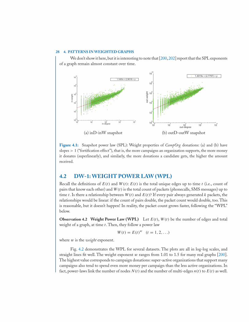
We don’t show it here,but it is interesting to note that [200,202] report that the SPL exponentsof a graph remain almost constant over time.

in-degree

in-w

eigh

t

1.1695x + (2.9019) = y

10010

0

102

104

106

108

1010

101

102

103

104

out-degree

out-

wei

ght

1.3019x + (2.7797) = y

10010

0

102

104

106

108

1010

101

102

103

104

(a) inD-inW snapshot (b) outD-outW snapshot

Figure 4.1: Snapshot power law (SPL): Weight properties of CampOrg donations: (a) and (b) haveslopes > 1 (“fortification effect”), that is, the more campaigns an organization supports, the more moneyit donates (superlinearly), and similarly, the more donations a candidate gets, the higher the amountreceived.

4.2 DW-1: WEIGHT POWER LAW (WPL)Recall the definitions of E(t) and W(t): E(t) is the total unique edges up to time t (i.e., count ofpairs that know each other) and W(t) is the total count of packets (phonecalls, SMS messages) up totime t . Is there a relationship between W(t) and E(t)? If every pair always generated k packets, therelationships would be linear: if the count of pairs double, the packet count would double, too. Thisis reasonable, but it doesn’t happen! In reality, the packet count grows faster, following the “WPL”below.

Observation 4.2 Weight Power Law (WPL) Let E(t), W(t) be the number of edges and totalweight of a graph, at time t . Then, they follow a power law

W(t) = E(t)w (t = 1, 2, . . .)

where w is the weight exponent.

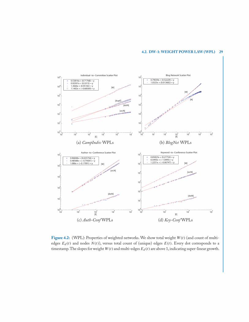
Fig. 4.2 demonstrates the WPL for several datasets. The plots are all in log-log scales, andstraight lines fit well. The weight exponent w ranges from 1.01 to 1.5 for many real graphs [200].The highest value corresponds to campaign donations: super-active organizations that support manycampaigns also tend to spend even more money per campaign than the less active organizations. Infact, power-laws link the number of nodes N(t) and the number of multi-edges n(t) to E(t) as well.

4.2. DW-1: WEIGHT POWER LAW (WPL) 29

102

103

104

105

106

10710

0

102

104

106

108

1010

1012Individual−to−Committee Scatter Plot

|E|

0.53816x + (0.71768) = y0.92501x + (0.3315) = y1.3666x + (0.95182) = y1.1402x + (−0.68569) = y |W|

|dupE|

|dstN|

|srcN|

100

101

102

103

104

105

10610

0

101

102

103

104

105

106 Blog Network Scatter Plot

|E|

0.79039x + (0.52229) = y1.0325x + (0.013682) = y

|N|

|W|

(a) CampIndiv WPLs (b) BlogNet WPLs

101

102

103

104

10510

0

101

102

103

104

105 Author−to−Conference Scatter Plot

|E|

0.96848x + (0.025756) = y0.48588x + (−0.74581) = y1.086x + (−0.17991) = y |W|

|srcN|

|dstN|

102

103

104

10510

0

101

102

103

104

105

106 Keyword−to−Conference Scatter Plot

|E|

0.85823x + (0.27754) = y0.5493x + (−1.0495) = y1.2251x + (−0.06747) = y

|srcN|

|dstN|

|W|

(c) Auth-Conf WPLs (d) Key-Conf WPLs

Figure 4.2: (WPL): Properties of weighted networks. We show total weight W(t) (and count of multi-edges Ed(t) and nodes N(t)), versus total count of (unique) edges E(t). Every dot corresponds to atimestamp.The slopes for weight W(t) and multi-edges Ed(t) are above 1, indicating super-linear growth.

30 4. PATTERNS IN WEIGHTED GRAPHS

4.3 DW-2: LWPL: WEIGHTED PRINCIPAL EIGENVALUEOVER TIME

Given that unweighted (0-1) graphs follow the λ1 Power Law (LPL, pattern D-5), one may ask ifthere is a corresponding law for weighted graphs.The answer is ’yes:’ let λ1,w be the largest eigenvalueof the weighted adjacency matrix Aw, where the entries wi,j of Aw represent the actual edge weightbetween node i and j (e.g., count of phone-calls from i to j ). Notice that λ1,w increases with thenumber of edges, following a power law with a higher exponent than that of its λ1 Power Law (seeFig. 4.3).

Observation 4.3 λ1,w Power Law (LWPL) Weighted real graphs exhibit a power law for thelargest eigenvalue of the weighted adjacency matrix λ1,w(t) and the number of edges E(t) over time.That is,

λ1,w(t) ∝ E(t)β

In the experiments in [200, 202], the exponent β ranged from 0.5 to 1.6.

|E|

λ 1, W

0.91595x + (2.1645) = y10

10

108

106

104

102

100

101

102

103

104

105

106

0.91595x + (2.1645) = y10

4

103

102

101

100

100

101

102

103

104

105

106

10-1

λ 1, W

|E|

0.69559x + (−0.40371) = y

λ 1,w

10

0.58764x + (-0.2863) = y3

102

101

101

102

10

|E|

310

410

510

0

(a) CampIndiv (b) BlogNet (c) Auth-Conf

Figure 4.3: Illustration of the LWPL. 1st eigenvalue λ1,w(t) of the weighted adjacency matrix Aw versusnumber of edges E(t) over time. The vertical lines indicate the gelling point.

31

C H A P T E R 5

Discussion—The Structure ofSpecific Graphs

While most graphs found naturally share many features (such as the small-world phenomenon),there are some specifics associated with each. These might reflect properties or constraints of thedomain to which the graph belongs. We will discuss some well-known graphs and their specificfeatures below.

5.1 THE INTERNETThe networking community has studied the structure of the Internet for a long time. In general, itcan be viewed as a collection of interconnected routing domains; each domain is a group of nodes(such as routers, switches, etc.) under a single technical administration [65]. These domains can beconsidered as either a stub domain (which only carries traffic originating or terminating in one of itsmembers) or a transit domain (which can carry any traffic). Example stubs include campus networks,or small interconnections of Local Area Networks (LANs). An example transit domain would be aset of backbone nodes over a large area, such as a wide-area network (WAN).

The basic idea is that stubs connect nodes locally, while transit domains interconnect the stubs,thus allowing the flow of traffic between nodes from different stubs (usually distant nodes). Thisimposes a hierarchy in the Internet structure, with transit domains at the top, each connecting severalstub domains, each of which connects several LANs.

Apart from hierarchy, another feature of the Internet topology is its apparent Jellyfish structureat the AS level (Figure 5.1), found by Tauro et al. [261]. This consists of:

• A core, consisting of the highest-degree node and the clique it belongs to; this usually has 8–13nodes.

• Layers around the core, organized as concentric circles around the core; layers further from thecore have lower importance.

• Hanging nodes, representing one-degree nodes linked to nodes in the core or the outer layers.The authors find such nodes to be a large percentage (about 40–45%) of the graph.

5.2 THE WORLD WIDE WEB (WWW)Broder et al. [61] find that the Web graph is described well by a “bowtie” structure (Figure 5.2(a)).They find that the Web can be broken into four approximately equal-sized pieces. The core of the

32 5. DISCUSSION—THE STRUCTURE OF SPECIFIC GRAPHS

CoreLayers

Hanging nodes

Figure 5.1: The Internet as a “Jellyfish:”The Internet AS-level graph can be thought of as a core, surroundedby concentric layers around the core. There are many one-degree nodes that hang off the core and eachof the layers.

bowtie is the Strongly Connected Component (SCC) of the graph: each node in the SCC has a directedpath to any other node in the SCC.Then, there is the IN component: each node in the IN componenthas a directed path to all the nodes in the SCC. Similarly, there is an OUT component, where eachnode can be reached by directed paths from the SCC. Apart from these, there are webpages whichcan reach some pages in OUT and can be reached from pages in IN without going through the SCC;these are the TENDRILS. Occasionally, a tendril can connect nodes in IN and OUT; the tendril iscalled a TUBE in this case. The remainder of the webpages fall in disconnected components. A similarstudy focused on only the Chilean part of the Web graph found that the disconnected componentis actually very large (nearly 50% of the graph size) [31].

Dill et al. [93] extend this view of the Web by considering subgraphs of the WWW at differentscales (Figure 5.2(b)). These subgraphs are groups of webpages sharing some common trait, such ascontent or geographical location. They have several remarkable findings:

1. Recursive bowtie structure: Each of these subgraphs forms a bowtie of its own. Thus, the Webgraph can be thought of as a hierarchy of bowties, each representing a specific subgraph.

2. Ease of navigation: The SCC components of all these bowties are tightly connected together viathe SCC of the whole Web graph. This provides a navigational backbone for the Web: startingfrom a webpage in one bowtie, we can click to its SCC, then go via the SCC of the entire Webto the destination bowtie.

3. Resilience: The union of a random collection of subgraphs of the Web has a large SCC com-ponent, meaning that the SCCs of the individual subgraphs have strong connections to otherSCCs. Thus, the Web graph is very resilient to node deletions and does not depend on theexistence of large taxonomies such as yahoo.com; there are several alternate paths betweennodes in the SCC.

5.2. THE WORLD WIDE WEB (WWW) 33

DisconnectedComponents

Tube

SCCOUTIN

TENDRILS

IN OUT

SCC

SCC

SCC

SCC

SCC

(a) The “Bowtie” structure (b) Recursive bowties

Figure 5.2: The “Bowtie” structure of the Web: Plot (a) shows the four parts: IN, OUT, SCC, andTENDRILS [61]. Plot (b) shows Recursive Bowties: subgraphs of the WWW can each be considered abowtie. All these smaller bowties are connected by the navigational backbone of the main SCC of theWeb [93].

35

C H A P T E R 6

Discussion—Power Laws andDeviations

6.1 POWER LAWS—SLOPE ESTIMATION

We saw many power laws in the previous sections. Here we describe how to estimate the slope of apower law, and how to estimate the goodness of fit. We discuss these issues below, using the detectionof power laws in degree distributions as an example.

Computing the power-law exponent: This is no simple task: the power law could be only in thetail of the distribution and not over the entire distribution, estimators of the power-law exponentcould be biased, some required assumptions may not hold, and so on. Several methods are currentlyemployed, though there is no clear “winner” at present.

1. Linear regression on the log-log scale: We could plot the data on a log-log scale, then optionally“bin” them into equal-sized buckets, and finally find the slope of the linear fit. However, thereare at least three problems: (i) this can lead to biased estimates [130], (ii) sometimes the powerlaw is only in the tail of the distribution, and the point where the tail begins needs to behand-picked, and (iii) the right end of the distribution is very noisy [215]. However, this isthe simplest technique, and seems to be the most popular one.

2. Linear regression after logarithmic binning: This is the same as above, but the bin widths increaseexponentially as we go toward the tail. In other words, the number of data points in each binis counted, and then the height of each bin is divided by its width to normalize. Plotting thehistogram on a log-log scale would make the bin sizes equal, and the power law can be fitted tothe heights of the bins.This reduces the noise in the tail buckets, fixing problem (iii). However,binning leads to loss of information; all that we retain in a bin is its average. In addition, issues(i) and (ii) still exist.

3. Regression on the cumulative distribution: We convert the pdf p(x) (that is, the scatter plot) intoa cumulative distribution F(x):

F(x) = P(X ≥ x) =∞∑

z=x

p(z) =∞∑

z=x

Az−γ (6.1)

36 6. DISCUSSION—POWER LAWS AND DEVIATIONS

The approach avoids the loss of data due to averaging inside a histogram bin. To see how theplot of F(x) versus x will look like, we can bound F(x):∫ ∞

x

Az−γ dz < F(x) < Ax−γ +∫ ∞

x

Az−γ dz

⇒ A

γ − 1x−(γ−1) < F(x) < Ax−γ + A

γ − 1x−(γ−1)

⇒ F(x) ∼ x−(γ−1) (6.2)

Thus, the cumulative distribution follows a power law with exponent (γ − 1). However, suc-cessive points on the cumulative distribution plot are not mutually independent, and this cancause problems in fitting the data.

4. Maximum-Likelihood Estimator (MLE): This chooses a value of the power law exponent γ

such that the likelihood that the data came from the corresponding power-law distribution ismaximized. Goldstein et al. [130] find that it gives good unbiased estimates of γ .

5. The Hill statistic: Hill [143] gives an easily computable estimator, that seems to give reliableresults [215]. However, it also needs to be told where the tail of the distribution begins.

6. Fitting only to extreme-value data: Feuerverger and Hall [116] propose another estimator whichis claimed to reduce bias compared to the Hill statistic without significantly increasing variance.Again, the user must provide an estimate of where the tail begins, but the authors claim thattheir method is robust against different choices for this value.

7. Non-parametric estimators: Crovella and Taqqu [89] propose a non-parametric method forestimating the power-law exponent without requiring an estimate of the beginning of thepower-law tail. While there are no theoretical results on the variance or bias of this estimator,the authors empirically find that accuracy increases with increasing dataset size, and that it iscomparable to the Hill statistic.

Checking for goodness of fit: The correlation coefficient has typically been used as an informalmeasure of the goodness of fit of the degree distribution to a power law. Recently, there has beensome work on developing statistical “hypothesis testing” methods to do this more formally. Beir-lant et al. [42] derive a bias-corrected Jackson statistic for measuring goodness of fit of the datato a generalized Pareto distribution. Goldstein et al. [130] propose a Kolmogorov-Smirnov testto determine the fit. Such measures need to be used more often in the empirical studies of graphdatasets.

6.2 DEVIATIONS FROM POWER LAWSWe saw several examples of power laws, and there are even more that we didn’t cover. Such examplesinclude the Internet AS1 graph with exponent 2.1 − 2.2 [115], the in-degree and out-degree dis-1Autonomous System, typically consisting of many routers administered by the same entity.

6.2. DEVIATIONS FROM POWER LAWS 37

tributions of subsets of the WWW with exponents 2.1 and 2.38 − 2.72 respectively [37, 61, 179],the in-degree distribution of the African web graph with exponent 1.92 [48], a citation graph withexponent 3 [237], distributions of website sizes and traffic [4], and many others. Newman [215]provides a long list of such works.

One may wonder: is every distribution a power law? If not, are there deviations? The answeris that, yes, there are deviations. In log-log scales, sometimes a parabola fits better, or some morecomplicated curves fit better. For example, Pennock et al. [231], and others, have observed deviationsfrom a pure power-law distribution in several datasets. Common deviations are exponential cutoffs,the so-called “lognormal” distribution, and the “doubly-Pareto-lognormal” distribution. We brieflycover them all, next.

6.2.1 EXPONENTIAL CUTOFFSSometimes the distribution looks like a power law over the lower range of values along the x-axis,but decays very quickly for higher values. Often, this decay is exponential, and this is usually calledan exponential cutoff:

y(x = k) ∝ e−k/κk−γ (6.3)

where e−k/κ is the exponential cutoff term and k−γ is the power-law term. Amaral et al. [23] findsuch behaviors in the electric power-grid graph of Southern California and the network of airports,the vertices being airports and the links being non-stop connections between them. They offer twopossible explanations for the existence of such cutoffs. One: high-degree nodes might have taken along time to acquire all their edges and now might be “aged,” and this might lead them to attractfewer new edges (for example, older actors might act in fewer movies). Two: high-degree nodesmight end up reaching their “capacity” to handle new edges; this might be the case for airportswhere airlines prefer a small number of high-degree hubs for economic reasons, but are constrainedby limited airport capacity.

6.2.2 LOGNORMALS OR THE “DGX” DISTRIBUTIONPennock et al. [231] recently found while the whole WWW does exhibit power-law degree distri-butions, subsets of the WWW (such as university homepages and newspaper homepages) deviatesignificantly. They observed unimodal distributions on the log-log scale. Similar distributions werestudied by Bi et al. [46], who found that a discrete truncated lognormal (called the Discrete GaussianExponential or “DGX” by the authors) gives a very good fit. A lognormal is a distribution whoselogarithm is a Gaussian; its pdf (probability density function) looks like a parabola in log-log scales.The DGX distribution extends the lognormal to discrete distributions (which is what we get indegree distributions), and can be expressed by the formula:

y(x = k) = A(μ, σ)

kexp

[− (ln k − μ)2

2σ 2

]k = 1, 2, . . . (6.4)

38 6. DISCUSSION—POWER LAWS AND DEVIATIONS

where μ and σ are parameters and A(μ, σ) is a constant (used for normalization if y(x) is aprobability distribution). The DGX distribution has been used to fit the degree distribution of abipartite “clickstream” graph linking websites and users (Figure 2.2(c)), telecommunications, andother data.

6.2.3 DOUBLY-PARETO LOGNORMAL (DPLN )Another deviation is well modeled by the so-called Doubly Pareto Lognormal (dPln). Mitzen-macher [210] obtained good fits for file size distributions using dPln. Seshadri et al. [245] studiedthe distribution of phone calls per customer, and also found it to be a good fit. We will describe theresults of Seshadri et al. below.

Informally, a random variable that follows the dPln distribution looks like the plots of Fig-ure 6.1: in log-log scales, the distribution is approximated by two lines that meet in the middle ofthe plot. More specifically, Figure 6.1 shows the empirical pdf (that is, the density histogram) for aswitch in a telephone company, over a time period of several months. Plot (a) gives the distributionof the number of distinct partners (“callees”) per customer.The overwhelming majority of customerscalled only one person; until about 80-100 “callees,” a power law seems to fit well; but after that,there is a sudden drop, following a power-law with a different slope. This is exactly the behavior ofthe dPln: piece-wise linear, in log-log scales. Similarly, Figure 6.1(b) shows the empirical pdf for thecount of phone calls per customer: again, the vast majority of customers make just one phone call,with a piece-wise linear behavior, and the “knee” at around 200 phone calls. Figure 6.1(c) shows theempirical pdf for the count of minutes per customer.The qualitative behavior is the same: piece-wiselinear, in log-log scales. Additional plots from the same source ([245]) showed similar behavior forseveral other switches and several other time intervals. In fact, the dataset in [245] included fourswitches, over month-long periods; each switch recorded calls made to and from callers who werephysically present in a contiguous geographical area.

PDF

Partners

DataFitted DPLN[2.8, 0.01, 0.35, 3.8]

10-6

10-4

10-2

102

103

100

101

104

PDF

Calls

DataFitted DPLN[2.8, 0.01, 0.55, 5.6]

100

10-6

10-4

10-2

102

103

104

105

PDF

Duration

DataFitted DPLN[2.5, 0.01, 0.45, 6.5]

10-6

10-4

10-2

102

104

(a) pdf of partners (b) pdf of calls (c) pdf of minutes

Figure 6.1: Results of using dPln to model. (a) the number of call-partners, (b) the number of calls made,and (c) total duration (in minutes) talked, by users at a telephone-company switch, during a given thetime period.

6.2. DEVIATIONS FROM POWER LAWS 39

For each customer, the following counts were computed:

• Partners: The total number of unique callers and callees associated with every user. Note thatthis is essentially the degree of nodes in the (undirected and unweighted) social graph, whichhas an edge between two users if either called the other.

• Calls: The total number of calls made or received by each user. In graph theoretic terms, thisis the weighted degree in the social graph where the weight of an edge between two users isequal to the number of calls that involved them both.

• Duration: The total duration of calls for each customer in minutes. This is the weighteddegree in the social graph where the weight of the edge between two users is the total durationof the calls between them.

The dPln Distribution For the intuition and the fitting of the dPln distribution, see the work ofReed [238]. Here, we mention only the highlights.

If a random variable X follows the four-parameter dPln distribution dPln(α, β, ν, τ ), thenthe complete distribution is given by:

fX = αβα+β

[e(αν+α2τ 2/2)x−α−1�(

log x−ν−ατ 2

τ) +

xβ−1e(−βτ+β2τ 2/2)�c(log x−ν+βτ 2

τ)], (6.5)

where � and �c are the CDF and complementary CDF of N(0, 1) (Gaussian with zero mean andunit variance). Intuitively, the pdf looks like a piece-wise linear curve in log-log scales; the parameterα and β are the slopes of the (asymptotically) linear parts, and ν and τ determine the knee of thecurve.

One easier way of understanding the double-Pareto nature of X is by observing that X canbe written as X = S0

V1V2

where S0 is lognormally distributed, and V1 and V2 are Pareto distributionswith parameters α and β. Note that X has a mean that is finite only if α > 1 in which case it is givenby

αβ

(α − 1)(β + 1)eν+ τ2

2 .

In conclusion, the distinguishing features of the dPln distribution are two linear sub-plots inthe log-log scale and a hyperbolic middle section.

191

Authors’ Biographies

DEEPAYAN CHAKRABARTIDr. Deepayan Chakrabarti obtained his Ph.D. from Carnegie Mellon University in 2005. He was aSenior Research Scientist with Yahoo, and now with Facebook Inc.He has published over 35 refereedarticles and is the co-inventor of the RMat graph generator (the basis of the graph500 supercomputerbenchmark). He is the co-inventor in over 20 patents (issued or pending). He has given tutorialsin CIKM and KDD, and his interests include graph mining, computational advertising, and websearch.

CHRISTOS FALOUTSOSChristos Faloutsos is a Professor at Carnegie Mellon University and an ACM Fellow. He hasreceived the Research Contributions Award in ICDM 2006, the SIGKDD Innovations Award(2010), 18 “best paper” awards (including two “test of time” awards), and four teaching awards.He has published over 200 refereed articles, and has given over 30 tutorials. His research interestsinclude data mining for graphs and streams, fractals, and self-similarity, database performance, andindexing for multimedia and bio-informatics data.

series issn: 2151-0067 sdynthesis s l ata ynthesis mining

Documents