service level expectation setting for air traffic management: … · 2019-02-20 · operational...
TRANSCRIPT

Service Level Expectation Setting for Air Traffic
Management: Project Overview
September 12, 2014
Sponsors: FAA Air Traffic Organization – Mission Support Services: Rich Jehlen, Rob Hunt, Yong Li
NEXTOR-II Team: Mike Ball, Alex Estes, Prem Swaroop, U of Maryland
Cindy Barnhart, Chiwei Yan, MITMark Hansen, Lei Kang, Yi Liu, UC Berkeley
Vikrant Vaze, Dartmouth

Current Practice on TMI Planning
2
TMI decisions
Strategic planning telecons

Operational Challenge
• Flight operators participate in strategic TMI planning by verbal input. Operators can sometimes have a disproportionate influence on decisions that affect a broad range of others who are less vocal.
• Discussion focuses on specific parameters rather than performance goals.
• Different traffic managers may create different plans for the same situation.
• The planning process is ad-hoc and subjective.
3
SLE Concept
• The Service Level Expectation (SLE) setting project has produced a conceptual approach and prototype software tool designed to address the above deficiencies.
• The SLE concept takes into account the input of all involved flight operators and generates an output that represents a consensus of those flight operators in making Traffic Flow Management Initiative (TMI) decision.
4

SLE Concept• The SLE mechanism allows
operators to submit quantitative input that represent their preferred system performance goals (capacity, predictability and efficiency).
• It then appropriately weighs and aggregates operators’ inputs to determine consensus performance goals.
• These goals can then used to determine TMI parameters that are expected to best achieve the performance expectations.
5
Underlying models, analysis and mechanisms are results of SLE project.
“Step 2”: requires additional research – performance based TMI planning.

A NextGen Vision: Performance-Based ATM
Philosophy:
• Airlines provide “consensus” service expectations
• FAA develops operational plan to meet those expectations
6
Expected Operating
Environment
Planned Operational
Response
Response Execution
Operational Outcome
Expected Operating
Environment
Service Expectations
Planned Operational
Response
Response Execution
Operational Outcome
Current Practice:
NextGen Vision:

COuNSEL: CONsensus Service Expectation Level Planning
Capacity
7
Efficiency
Information to users:
candidate performance vectors
Predictability
V1: 0.9 0.8 0.5
V2: 0.7 0.7 0.9
V3: 0.8 0.6 0.8
Grades:
Inputs from user 1:
Grades for vectors
and candidate vectors
100%, 95%, 90%, 85% …
Consensus vector:
e.g. (.89 , .76 , .65)

Consensus Vector Chosen using Majority Judgment
• Suppose:– 6 airlines (voters), voting on 3 candidates: V1, V2, V3
– grades: 100%, 99%, 98%, 97%, 96%, 95%, 94%, …
• Grades sorted after voting from worst to best:
8
V1 80% 80% 90% 94% 95% 100%
V2 75% 83% 85% 87% 88% 90%
V3 65% 70% 88% 90% 93% 95%
Majority grades: majority would give at least that grade.…. in this example 4th grade from right.Vector with highest majority grade will be selected.There is a tie-breaking rule – not discussed here.
Performance Goals in SLE
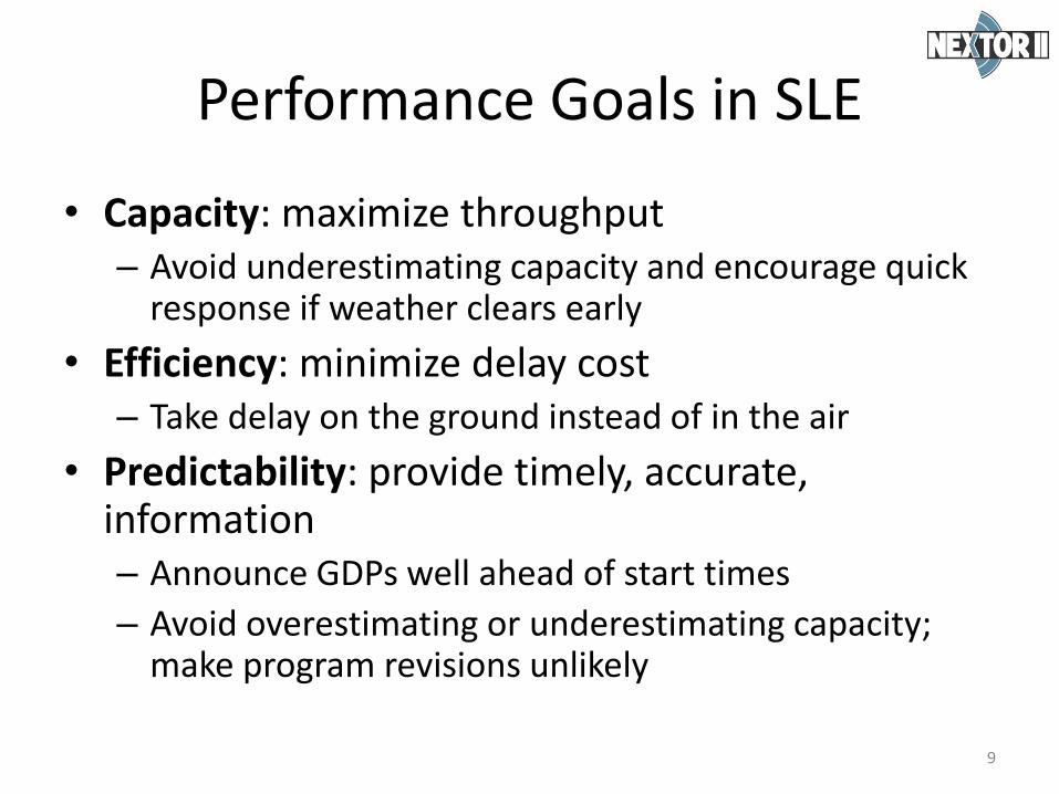
• Capacity: maximize throughput– Avoid underestimating capacity and encourage quick
response if weather clears early
• Efficiency: minimize delay cost– Take delay on the ground instead of in the air
• Predictability: provide timely, accurate, information– Announce GDPs well ahead of start times
– Avoid overestimating or underestimating capacity; make program revisions unlikely
9

Interpretation of Performance Goals
All metrics take on values between 0 and 11 perfect performance
0 worst possible performance
The system only allows goal vectors that are “feasible”, e.g. even on a near-perfect day (1,1,1) would not be possible – perfect performance across all dimensions.
The system forces the flight operators to make tradeoffs:
(.91, .83, .85) (.86, .89, .85)
Reduce capacity goal: .91 .86
… in order to improve efficiency goal: .83 .89
10

Interpretation of Performance Goals
Capacity: 1 maximum airport throughput achieved (perfect weather day)
As metric decreases, flights will be delayed, cancellations may be necessary, diversions are a possibility, etc.
11

Interpretation of Performance Goals
Efficiency: 1 each flight will be executed in a minimum (user) cost manner: no airborne holding or vectoring, minimum taxi-in/out times, no diversions (note: an assigned ground delay is not counted against user cost as this cost is captured under capacity/throughput)
As metric decreases, airborne delays (and diversions) become more likely, the need to take suboptimal routes becomes more likely, etc.
12
Interpretation of Performance Goals
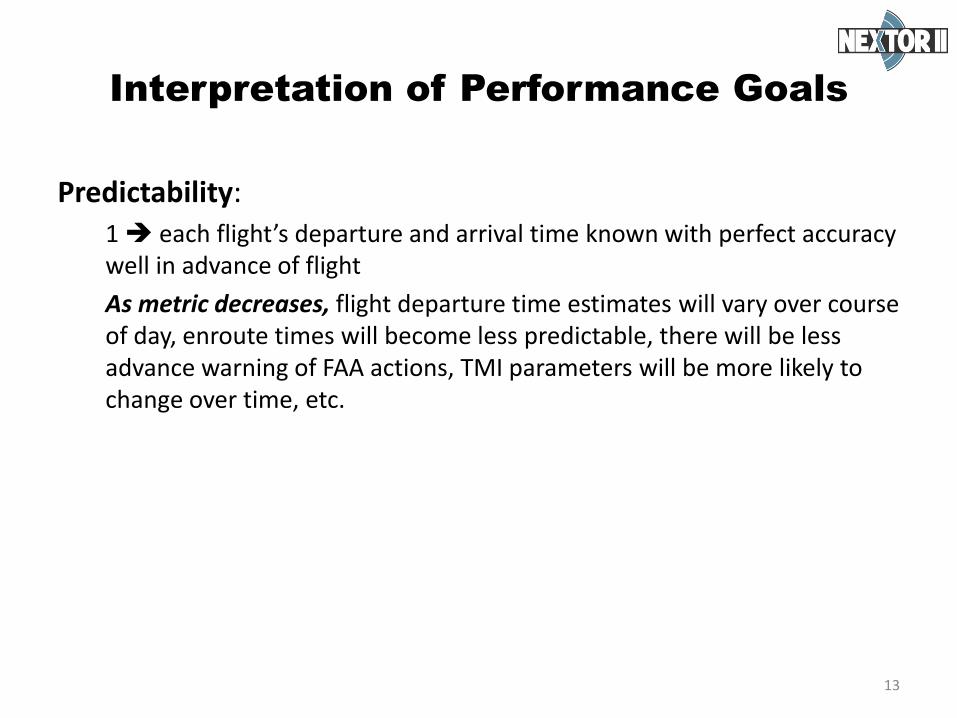
Predictability:1 each flight’s departure and arrival time known with perfect accuracy well in advance of flight
As metric decreases, flight departure time estimates will vary over course of day, enroute times will become less predictable, there will be less advance warning of FAA actions, TMI parameters will be more likely to change over time, etc.
13

Design Tradeoffs• SLE will enable flight operators to influence TMI design tradeoffs• Predictability vs. Throughput
– Predictability— assume lower rates and long duration so that initially assigned delays are unlikely to be extended
– Throughput—assume higher rates and shorter duration in order to increase demand pressure
• Efficiency vs. Throughput– Efficiency—minimize airborne delay by imposing more ground delay– Throughput—employ higher arrival rates to increase demand
pressure but (possibly) at the expense of more airborne delay
• Predictability vs. Efficiency– Predictability—make decisions well in advance, even though this
increases the risk that they will be based on erroneous forecasts– Efficiency—make decisions later when better information is available,
reducing the risk of airborne delay
14

SLE Features
• Airline votes are weighted by number of flights involved in the TMI
• Voting process is iterative—new candidate vectors are determined by ratings of previous candidate vectors
• Only feasible candidate vectors are allowed — set of feasible vectors is based on conditions of the day
• Airlines may develop their own tools to assess how different candidate vectors affect their individual business objectives
• Multiple applications of COuNSEL might be used as conditions change; could be applied nationwide or to regional problem area
15

ANSP InputCandidatesWeights
Service
Expectations
Resolution
Winner
Feasibility Constraints
16
Airline InputGradesCandidates
ANSP ProcessingGrade function estimationNew candidate generation
COuNSEL Logic Flow
Significant Research Components
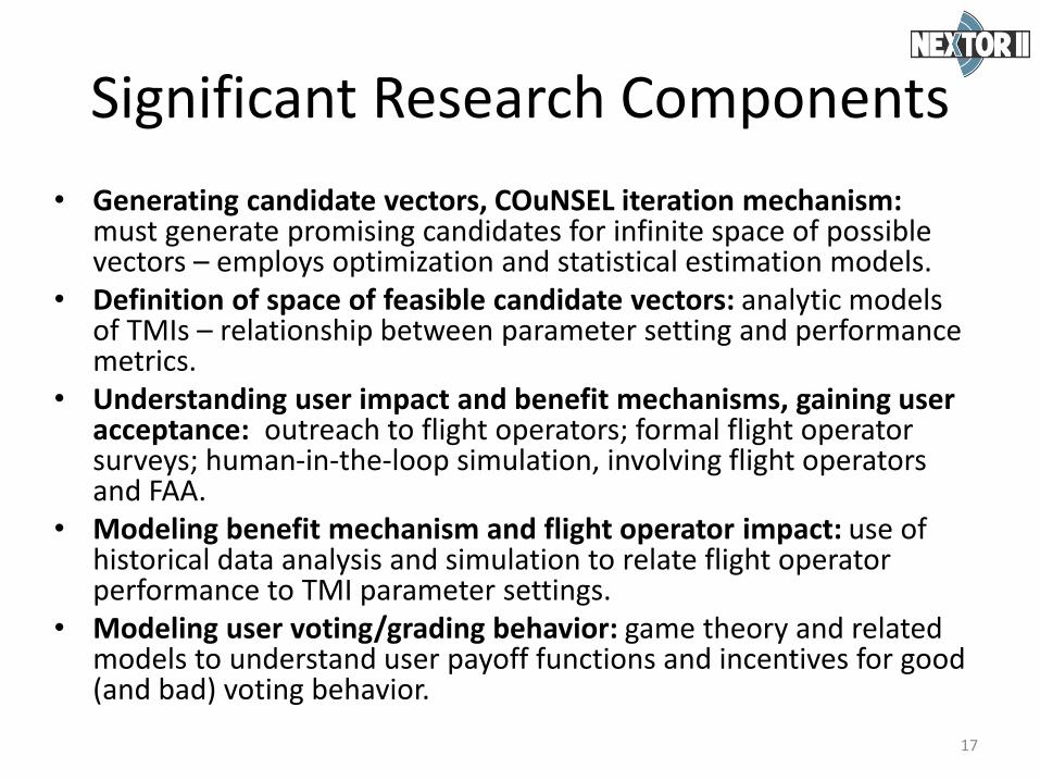
• Generating candidate vectors, COuNSEL iteration mechanism: must generate promising candidates for infinite space of possible vectors – employs optimization and statistical estimation models.
• Definition of space of feasible candidate vectors: analytic models of TMIs – relationship between parameter setting and performance metrics.
• Understanding user impact and benefit mechanisms, gaining user acceptance: outreach to flight operators; formal flight operator surveys; human-in-the-loop simulation, involving flight operators and FAA.
• Modeling benefit mechanism and flight operator impact: use of historical data analysis and simulation to relate flight operator performance to TMI parameter settings.
• Modeling user voting/grading behavior: game theory and related models to understand user payoff functions and incentives for good (and bad) voting behavior.
17

Benefits of SLE
• A more fair and inclusive decision-making process where all the flight operators’ voices will be heard
• A goal-oriented decision-making process where performance criteria are clear to the flight operators
• A more consistent decision-making process where decision are less dependent on managers’ experience and personality
18

Topic 1: Choice of Performance Categories

NextGen: Performance-Based ATM
• “Performance based” ATM for National Air Space (NAS)
– Support airline operators’ business objectives subject only to system-level objectives like safety and security
• Consistent with global and other regions’ visions of future ATM
20
1. Capacity2. Cost-effectiveness3. Efficiency4. Flexibility5. Predictability
6. Access & Equity7. Environment8. Global interoperability9. Participation by the ATM Community10.Security11.Safety
Expected Operating
Environment
Service Expectations
Planned Operational
Response
Response Execution
Operational Outcome

NextGen: Performance-Based ATM
• “Performance based” ATM for National Air Space (NAS)
– Support airline operators’ business objectives subject only to system-level objectives like safety and security
• Consistent with global and other regions’ visions of future ATM
21
1. Capacity2. Cost-effectiveness3. Efficiency4. Flexibility5. Predictability
6. Access & Equity7. Environment8. Global interoperability9. Participation by the ATM Community10.Security11.Safety
Expected Operating
Environment
Service Expectations
Planned Operational
Response
Response Execution
Operational Outcome
Chosen

NextGen: Performance-Based ATM
• “Performance based” ATM for National Air Space (NAS)
– Support airline operators’ business objectives subject only to system-level objectives like safety and security
• Consistent with global and other regions’ visions of future ATM
22
1. Capacity2. Cost-effectiveness3. Efficiency4. Flexibility5. Predictability
6. Access & Equity7. Environment8. Global interoperability9. Participation by the ATM Community10.Security11.Safety
Expected Operating
Environment
Service Expectations
Planned Operational
Response
Response Execution
Operational Outcome
These would be set as global/strategic requirements and not manipulated on a day to day basis.

NextGen: Performance-Based ATM
• “Performance based” ATM for National Air Space (NAS)
– Support airline operators’ business objectives subject only to system-level objectives like safety and security
• Consistent with global and other regions’ visions of future ATM
23
1. Capacity2. Cost-effectiveness3. Efficiency4. Flexibility5. Predictability
6. Access & Equity7. Environment8. Global interoperability9. Participation by the ATM Community10.Security11.Safety
Expected Operating
Environment
Service Expectations
Planned Operational
Response
Response Execution
Operational Outcome
Refers to ANSP cost effectiveness; not likely that flight operators would have incentive to reduce this.

NextGen: Performance-Based ATM
• “Performance based” ATM for National Air Space (NAS)
– Support airline operators’ business objectives subject only to system-level objectives like safety and security
• Consistent with global and other regions’ visions of future ATM
24
1. Capacity2. Cost-effectiveness3. Efficiency4. Flexibility5. Predictability
6. Access & Equity7. Environment8. Global interoperability9. Participation by the ATM Community10.Security11.Safety
Expected Operating
Environment
Service Expectations
Planned Operational
Response
Response Execution
Operational Outcome
There could be good arguments for including, e.g. TMI designs that allow flight operators greater ability to substitute and internally optimize would certainly be viewed positively.

NextGen: Performance-Based ATM
• “Performance based” ATM for National Air Space (NAS)
– Support airline operators’ business objectives subject only to system-level objectives like safety and security
• Consistent with global and other regions’ visions of future ATM
25
1. Capacity2. Cost-effectiveness3. Efficiency4. Flexibility5. Predictability
6. Access & Equity7. Environment8. Global interoperability9. Participation by the ATM Community10.Security11.Safety
Expected Operating
Environment
Service Expectations
Planned Operational
Response
Response Execution
Operational Outcome
Important category; however, flight operators would vote based on whether they were currently getting good or bad end of inequitable treatment; perhaps ANSP should somehow control equity metric.

Specific Metrics
• The metrics used in each category were chosen for specific reasons related to status of research and prototype development:
– We anticipate that these will change based on more research and priorities set by various other groups within the FAA.
26

Topic 2: Choice of Underlying Mechanism
Swaroop and Ball | Apr 21, 2012 | POMS, Chicago

Research Problem
• Design a consensus-building mechanism,incorporating airline operators’ preferences,for determining the levels of serviceexpectations at NAS-level, usable by the AirNavigation Service Provider (ANSP), to designPlanned Operational Response, for the day-of-operations
Swaroop and Ball | Apr 21, 2012 | POMS, Chicago
28

Desirable Properties
1. single winner determination.– Leads to a unique “winner”.
2. confidentiality.– Minimal private information requirements from the airlines.
3. practicality.– Easy to administer, not involving time-consuming information
gathering and / or processing steps.
4. consensus-building.– Maximum acceptability among the airlines.
5. equitability.– Perceived to be fair to all parties involved from the outset.
6. strategy-proof.– As far as possible, encourage truth-telling behavior.
Swaroop and Ball | Apr 21, 2012 | POMS, Chicago
29

Mechanisms Considered
• “Investment” / Marketplace / Combinatorial Auction– Requires creation of artificial “currency”– Metrics are not really goods being split up
• Strategic behavior unavoidable: free-rider problem
• Multi-player Non-cooperative Game– Useful in modeling the strategic behavior– Existence of unique Nash equilibrium established– Outcomes not “desirable”: extreme solutions, without desired tradeoffs
• Voting– Natural way to model the decision making paradigm– Challenges exist in modeling– Two alternatives considered:
• Weighted Instant Runoff Voting• Majority Judgment
– Game theory to be used for analysis30

Majority Judgment
• Recently proposed procedure (Balinski and Laraki, ‘10)
• Bypasses Arrow’s Impossibility Theorem (1950)– when voters have three or more distinct alternatives, no
voting system can convert the ranked preferences of individuals into a community-wide (complete and transitive) ranking while also meeting a certain set of criteria, namely: unrestricted domain, non-dictatorship, Pareto efficiency, and independence of irrelevant alternatives.
• Claimed by authors to be “a better alternative to all other known voting methods, in theory and in practice.”
31

Majority Judgment – Definition
Majority Judgment is a social decision function
• Grading of each candidate by all voters in a common language– instead of preference rankings
– more natural, richer preference elicitation
• Many good properties: highly resistant to strategic voting
32
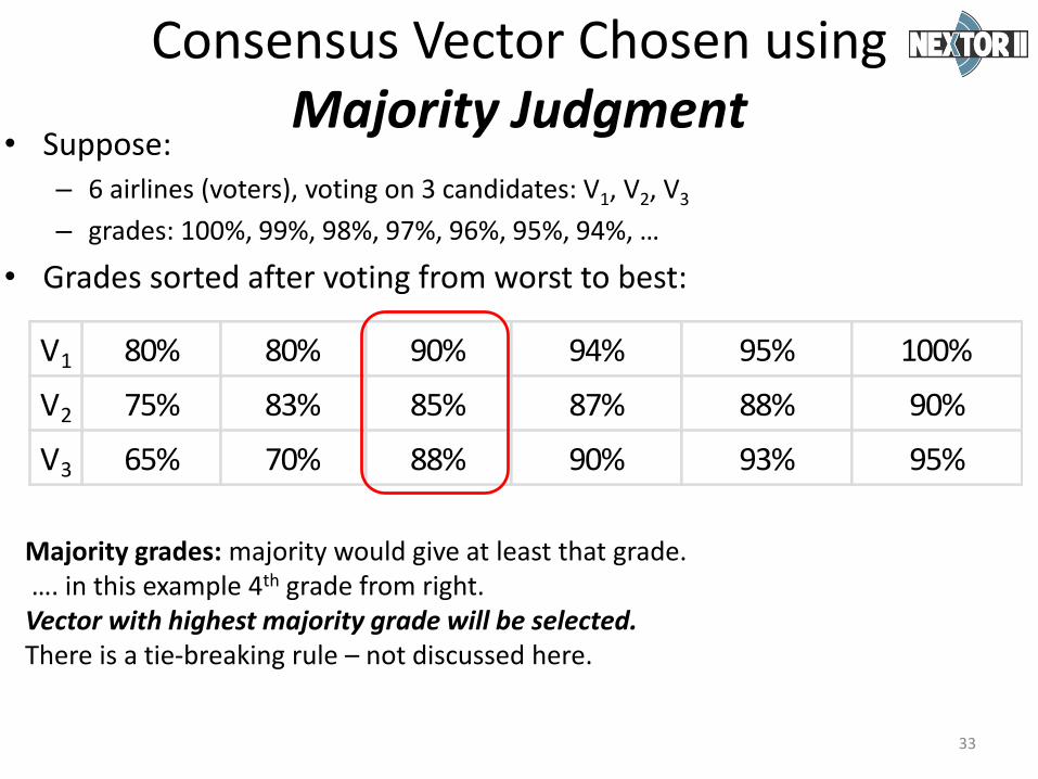
Consensus Vector Chosen using Majority Judgment
• Suppose:– 6 airlines (voters), voting on 3 candidates: V1, V2, V3
– grades: 100%, 99%, 98%, 97%, 96%, 95%, 94%, …
• Grades sorted after voting from worst to best:
33
V1 80% 80% 90% 94% 95% 100%
V2 75% 83% 85% 87% 88% 90%
V3 65% 70% 88% 90% 93% 95%
Majority grades: majority would give at least that grade.…. in this example 4th grade from right.Vector with highest majority grade will be selected.There is a tie-breaking rule – not discussed here.

MJ in Perspective• The use of the median grade as the majority grade is key to the
good properties of MJ, i.e. it greatly reduces the potential gain from “strategic” grading. …. Yet, in terms of global welfare, one would prefer the average grade.Even in the limited set of examples explored in the HITL, this issue was very notable to participants (and made some participants question the MJ criterion).
34
Idea worth exploring: use median criterion to identify set of nearly equivalent vectors and allow ANSP to break near-ties using other criteria, e.g. average grade, equity, etc.
Idea worth exploring: use median criterion to identify set of nearly equivalent vectors and allow ANSP to break near-ties using other criteria, e.g. average grade, equity, etc.
35

Topic 3: Majority Judgment –Adaptation for Use in COuNSEL

Challenge in Application of MJ to Service Level Expectation Setting
• The basic application of MJ allows flight operators to make a consensus choice among possible goal vectors.
• Challenge 1: given conditions on a particular day of operations what are appropriate “possible goal vectors” that should be presented to flight operators.
– Partial Answer: In concept there will be many (an infinite number) of vectors that represent the possible tradeoffs among the performance vectors given the weather and traffic conditions for the scenario of interest. Thus, challenge 1, becomes the problem of representing the space of performance metric tradeoffs for the TMIs under consideration.
• Challenge 2: given some representation of the space of possible goal vectors, what is a process for choosing among these the ones that flight operators will grade as part of the MJ process?
37

Solution to Challenge 1: Set of constraints that define feasible vectors for particular day in the NAS.
Bad weather day – sample vectors: (.90, .75, .80), (.85, .80, .83), (.85, .90, .79).
Good weather day – sample vectors: (.98, .95, .90), (.99, .92, .91), (.95, .97, .90).
38
m is possible metric vector :
𝐦 ∈ 𝐹𝐸𝐴𝑆𝑀𝐸𝑇𝑅𝐼𝐶

Majority Judgment (with small set of vectors)
• Suppose:– 6 airlines (voters), voting on 3 candidates: V1, V2, V3
– grades: 100%, 99%, 98%, 97%, 96%, 95%, 94%, …
• Grades sorted after voting from worst to best:
39
V1 80% 80% 90% 94% 95% 100%
V2 75% 83% 85% 87% 88% 90%
V3 65% 70% 88% 90% 93% 95%
Majority grades: majority would give at least that grade.…. in this example 4th grade from right.Vector with highest majority grade will be selected.There is a tie-breaking rule – not discussed here.

COuNSEL Architecture
40
Feasibility Constraints
Airline 1 Input• Grades• Candidates
Service Expectations Resolution (Majority
Judgment)
Evaluation /Generation of New
Candidates
Airline 1 Assessment
Airline Weights(Fn. of num. flts. impacted)
ANSP Input

Applying MJ with infinite set of
candidates:
1. Define optimization model (MJ-Opt) that finds Majority Judgment winner assuming each airline’s grading function 𝑔𝑎 𝐦 is known.
2. Iteratively generate candidate vectors and based on airline grades use statistical methods to estimate 𝑔𝑎 𝐦– Candidate generation employs MJ-Opt to generate candidates
likely to be close to MJ winner.
Also:
Allow flight operators to supply their own candidates.
41

Majority Judgment Winner
all possible candidates
“best” majority-forming set involving each player(Player_Opt(i’))
all possible majority-forming sets(Subset_Opt(b))
“Majoritarian Set”: set of players that determine MG
Player with the lowest grade in MS determines MG
Candidate with the highest MG wins42

1
2
31
2
3
1
2
31
2
3
43
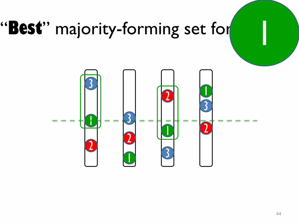
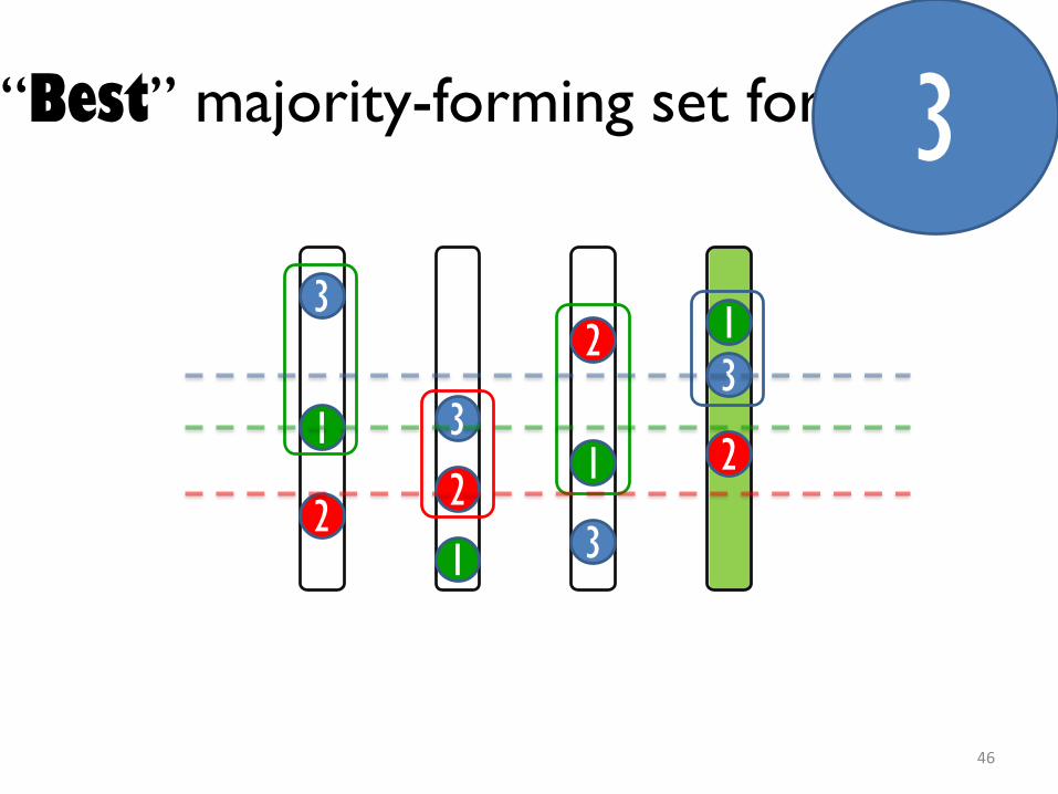
“Best” majority-forming set for a player
1
2
31
2
3
1
2
31
2
3
44
“Best” majority-forming set for a player1
1
2
31
2
3
1
2
31
2
3
45
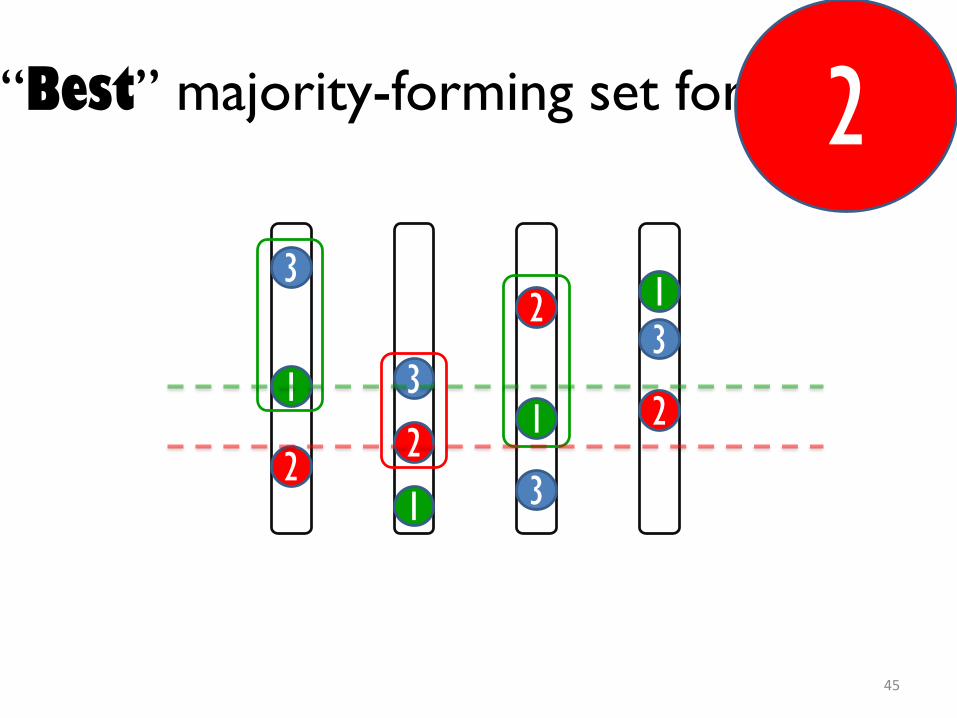
“Best” majority-forming set for a player2
1
2
31
2
3
1
2
31
2
3
46
“Best” majority-forming set for a player3
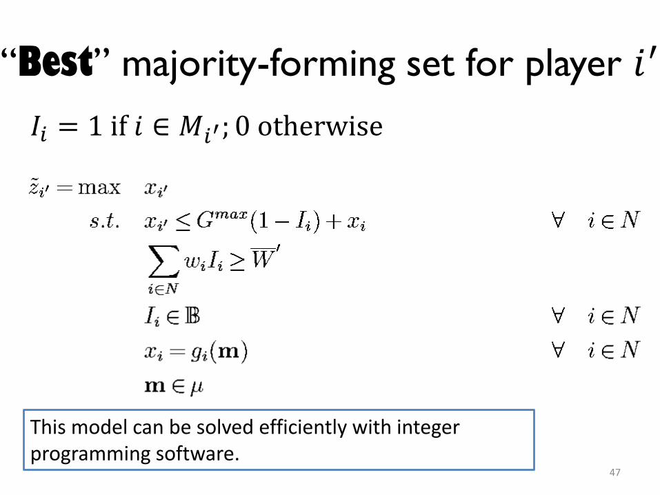
𝐼𝑖 = 1 if 𝑖 ∈ 𝑀𝑖′; 0 otherwise
47
“Best” majority-forming set for player 𝑖′
This model can be solved efficiently with integer programming software.

𝐼𝑎 = 1 if 𝑎 ∈ 𝑀𝑎′; 0 otherwise
Majority Judgment Winner
Candidate with the highest MG wins48
“best” majority-forming set involving each player(Player_Opt(i’))

^
Estimate grade function
Constrained least-squares regression (for concavity)49
“Best” majority-forming set for player 𝑖′
𝐼𝑖 = 1 if 𝑖 ∈ 𝑀𝑖′; 0 otherwise
New Candidate Vectors

Same formulation: Two Uses
1. Majority Judgment Winner determination over
continuous candidate spaceUses knowledge of grade functions
Theoretical
2. New candidate generationEstimates grade functions (constrained least-squares)
Practical
50

Chicago area (ORD + MDW)
October 2007
51
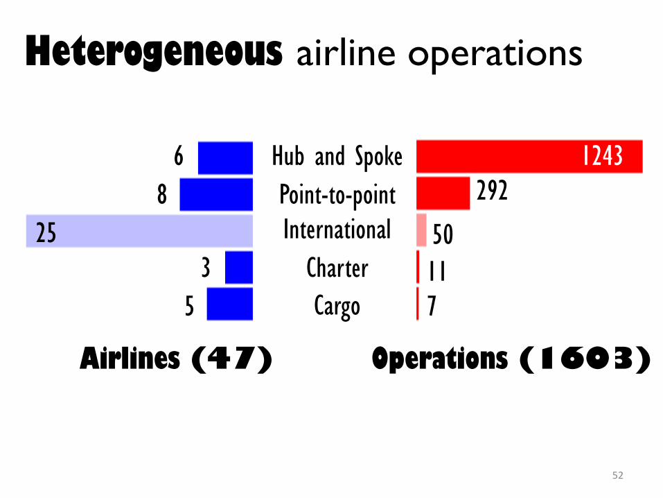
Hub and Spoke
Point-to-point
International
Charter
Cargo
6
8
25
3
5
1243
292
50
11
7
Heterogeneous airline operations
Airlines (47) Operations (1603)
52

UAAAWNNWDLUSCOFL
20
19
635500
242
2827
34
1918
Long tail in distribution of operations
53

Airlines’ best vectors are spread out
54
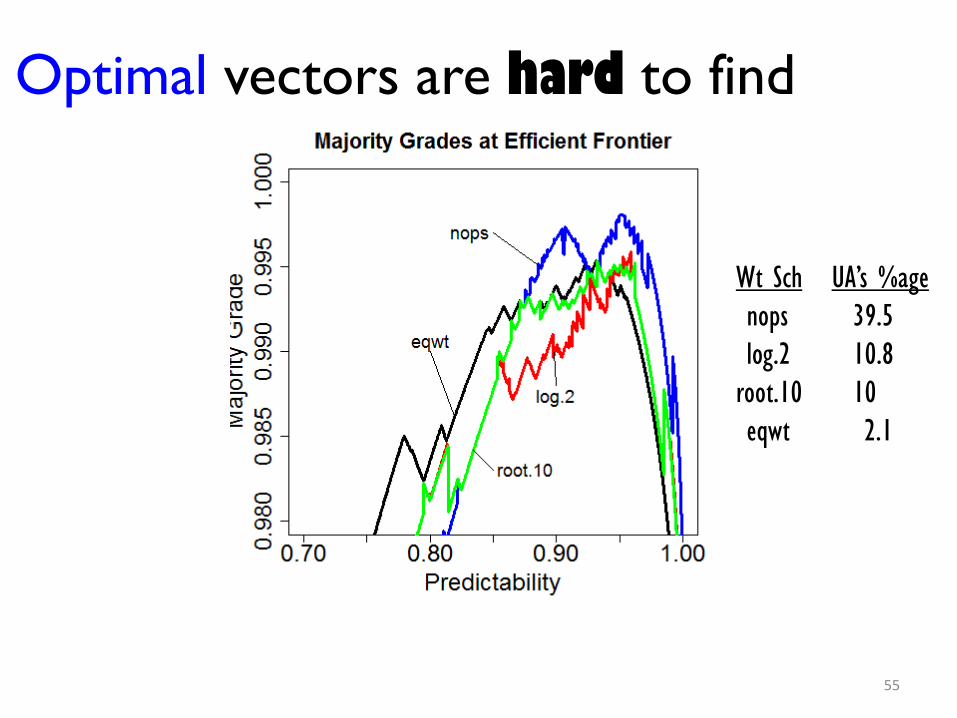
Optimal vectors are hard to find
Wt Sch UA’s %age
nops 39.5
log.2 10.8
root.10 10
eqwt 2.1
55

Winning vectors are close to Optimal
Overall accuracy of procedure: 0.2%56

Computing times are manageable
Dell Inspiron 5520
Intel Core i7-3612 @2.10GHz,, 8GB RAM
Windows 7 Ultimate 64-bit
R 2.15.1 32-bit
CPLEX 12.4 via Rcplex 0.3-0
quadprog 1.5-457

Final Thoughts
• Simulation has shown approach to be computationally effective for 2-metric spaces – have not fully tested process for 3-dimensional vectors but looks quite doable.
• Practical Perspective: as was done in the HITL, the system can work quite well with “more modest” ways of generating candidate vectors, e.g. allowing flight operators to submit candidates, creating list ahead of time based on intuition, using various “heuristic” criteria.
… the sophisticated integer programming approach to candidate generation may not be critical in practice (but determining this will require more experimentation).
58

Topic 4: Definition of Space of Feasible Candidate Vectors
59

Characteristics of Space of Feasible Performance Goal Vectors:
• A basic assumption of the performance metrics is a higher value of any metric is preferred to a lower value (by any flight operator), e.g. any flight operator would prefer (.91, .88, .85) to (.91, .82, .85) since the first and last metric values are the same but the 2nd is higher in the first vector (we say the 1st point dominates the 2nd).
• Also, it is assumed (somewhat for conceptual and mathematical convenience) that if two vectors are possible/feasible then any vector on the line segment between them is feasible, e.g. if (.91, .88, .87) and (.91, .82, .91) are both feasible then a point in between, e.g. ½ (.91, .88, .87) + ½ (.91, .82, .91) = (.91, .85, .89) is also feasible.
60
V1
V2
Dominatedpoints
V1
V2
Dominatedpoints
All feasible

Characteristics of Space of Feasible Performance Goal Vectors
• Thus we can define the space of feasible vectors by a set of linear constraints with the structure illustrated below
• Only the points of the efficient frontier are of interest as possible goal vector
61
V1
V2
Points on the efficient frontierDominated points

Format of Constraints Defining Space of Performance Goal Vectors• Based on the previous discussion, if
performance vectors are denoted by (V1, V2, V3) then any constraint defining the region of feasible performance goal vectors has the form:
A1 V2 + A2 V2 + A3 V3 <= B
where A1, A2, A3 >= 0 and B > 0
• The COuNSEL software tool accepts a list of constraints in this format.
62

Generating Constraints
• Approach to generating constraints defining space of feasible performance vectors:
– Step 1: generate set of possible performance vectors given the weather and demand conditions of the day.
– Step 2: find set of constraints that encloses the points generated in step 1, in a feasible region with the appropriate properties.
63

Solution to Step 2• There are well known methods that find a set of constraints defining the
convex hull of a set of given points – such methods can be accessed as functions in various computational toolkits
• This “almost” provides a solution to Step 2: before applying such a method, it may be necessary to add some points to insure the set of points have the structured described earlier.
• The figure below illustrates the points that may need to be added.
64V1
V2 Added points The points added insure that all dominated are feasible and that the interior constraints defining the region contain only non-dominated points

Solution to Step 1: Performance Vector Generation for GDPs
Based on Analysis of Historical Days
• Research carried out so far assumes a GDP plan is characterized (only) by the planned airport arrival rate vector (PAAR)
• The performance achieved by choosing a particular PAAR is determined by the actual airport arrival capacity profile that occurs (AAAR)
• The conditions on a particular day (weather forecast) will determine an AAAR distribution for that day, i.e. a list of possible AAAR together with associated probabilities
• Performance vectors can be enumerated by enumerating possible PAARs and computing an associated performance vector for each PAAR by applying the AAAR distribution
65

The Logic
• Identify a set of possible capacity profiles for the given day-of-operation
• Each possible capacity profile may be selected as the planned capacity profile
66

The Logic (II)
• For each planned capacity profile, the feasible candidate vector (SLE metric) is estimated as an average of the realized system performances over all the possible capacity profiles that may realize:
𝑀𝑖𝑘 =
σ𝑗=1𝐽
𝑀𝑖,𝑗𝑘
𝐽
where, 𝑀𝑖𝑘 is SLE metric for performance goal 𝑘 with
planned capacity profile 𝑖;
𝑀𝑖,𝑗𝑘 is the realized performance for performance goal
𝑘 if capacity profile 𝑖 is planned and capacity profile 𝑗 is the actual capacity profile.
67

Flowchart
68
Actual capacity profile 1
Planned start time &
end time
Exemption criteria
&Planned capacity profile 𝑖
1
Actual capacity profile 𝐽
𝐽
𝑀𝑖,11 ,𝑀𝑖,1
, 𝑀𝑖,1 )
𝑀𝑖,𝐽1 , 𝑀𝑖,𝐽
, 𝑀𝑖,𝐽 )
SLE metric vector:
𝑀𝑖1, 𝑀𝑖
,𝑀𝑖 = 𝑗 𝑀𝑖,𝑗
1 , 𝑀𝑖,𝑗 , 𝑀𝑖,𝑗
) 𝐽
𝑗=1
Initial assignment of time slots
Demand
GDP design:
Demand
Demand
Currently, all the profiles are assumed to be equally likely.
Performance Goals
• Currently, we are considering the following performance criteria:
– Capacity utilization
– Efficiency
– Predictability
• More criteria could be considered upon users’ request
69

Capacity Utilization
This metric is defined to measure how much capacity is planned when the GDP is first implemented against the capacity under VMC condition:
𝑀𝑖,𝑗1 = 𝛼𝑐𝑢,𝑖,𝑗 =
𝑁𝑅,𝑖,𝑗
𝑁𝑉𝑀𝐶,𝑖,𝑗
where,
𝛼𝑐𝑢,𝑖,𝑗 is the capacity utilization metric with planned capacity profile 𝑖and actual capacity profile 𝑗;
𝑁𝑅,𝑖,𝑗is the count of realized arrivals between GDP start time and end time when capacity profile 𝑖 is planned and profile 𝑗 is realized;
𝑁𝑉𝑀𝐶,𝑖,𝑗 is the count of arrivals that could have been landed assuming VMC capacity and infinite demand during the same period for the same pair of profiles.
70

Efficiency
Efficiency is defined referring to the motivation of GDP: transforming airborne delay to cheaper ground delay:
𝑀𝑖,𝑗 = 𝛼𝑒,𝑖,𝑗 =
σ𝑘 𝐺𝐷𝑖,𝑗,𝑘
σ𝑘 𝑇𝐷𝑖,𝑗,𝑘
where,
𝛼𝑒,𝑖,𝑗 is the efficiency metric with planned capacity profile 𝑖 and actual capacity profile 𝑗;
𝐺𝐷𝑖,𝑗,𝑘 is the ground delay incurred by flight 𝑘 for the same pair of capacity profiles;
𝑇𝐷𝑖,𝑗,𝑘 is the total delay incurred by flight 𝑘, equal to realized ground delay plus realized airborne delay.
71

Predictability
• Predictability is defined to capture the accuracy in estimating capacity rates. In the strategic planning telecons, most of the debate is on setting capacity rates.
• On one hand, we want to make sure available capacity will be effectively utilized. On the other hand, we also appreciate the accuracy of the guess on capacity rates. The former is considered in the capacity utilization and the latter is considered by predictability metric.
72

Predictability (II)
𝑀𝑖,𝑗 = 𝛼𝑝,𝑖,𝑗 =
1
𝑇σ𝑡=1
𝑇 𝑚𝑖𝑛 𝑃𝐴𝐴𝑅𝑖,𝑡,𝐴𝐴𝐴𝑅𝑗,𝑡
𝑚𝑎𝑥 𝑃𝐴𝐴𝑅𝑖,𝑡,𝐴𝐴𝐴𝑅𝑗,𝑡
where,
𝛼𝑝,𝑖,𝑗 is the predictability metric with planned capacity profile 𝑖 and actual capacity profile 𝑗; 𝑡 is the index for the 15-minute interval and 𝑇 is the total number of intervals; 𝑃𝐴𝐴𝑅𝑖,𝑡 is the planned airport acceptance rate for interval 𝑡 given plan capacity profile as 𝑖;
𝐴𝐴𝐴𝑅𝑗,𝑡 is the actual airport acceptance rate for interval 𝑡when the actual capacity profile is 𝑗.
73
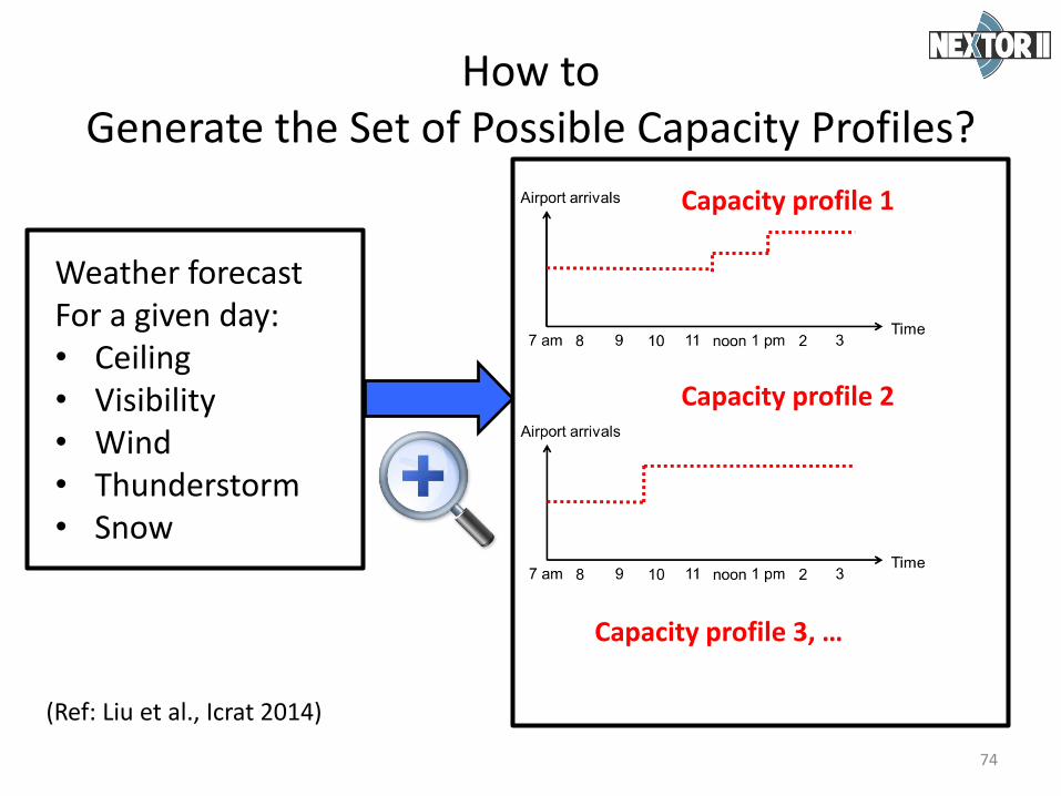
How to Generate the Set of Possible Capacity Profiles?
74
Weather forecastFor a given day:• Ceiling• Visibility• Wind• Thunderstorm• Snow
Capacity profile 1
Capacity profile 2
Capacity profile 3, …
(Ref: Liu et al., Icrat 2014)

Methodology:learn from history
75

Logic in the Method
76
Given day
Historical days
Day G
Day H1 Day H2 … Day Hm
Total distances 𝑇𝐷𝐺,𝐻1𝑇𝐷𝐺,𝐻2
… 𝑇𝐷𝐺,𝐻𝑚
Similarity Highest Lowest
< < <
Closest Furthest
Capacity profiles Profile 1 Profile mProfile 2 …×√ √
𝑇𝐷𝐺,𝐻𝑖:Total distance in weather forecast
between Day G and Day Hi

Total distance between Days G and H
77
timestart end
Day G:
timestart end
Day H:
hours
𝑑1
1 2 n
1 2 n
𝑑
𝑑𝑛
𝑇𝐷𝐺,𝐻 = σ𝑖=1𝑛 𝑑𝑖
hourly distances
in
weather forecasts

Hourly Distance between Hours j and k
78
𝑑𝑗,𝑘 𝐴 = 𝑊𝐹𝑗 − 𝑊𝐹𝑘 𝑇 ∙ 𝐴 ∙ 𝑊𝐹𝑗 − 𝑊𝐹𝑘
Weather Forecast vector[x1, x2, x3]
Matrix of distance coefficients
∆x1 ∆x2 ∆x3
∆x1
∆x2
∆x3
a1,1
a2,1
a3,1
a1,2
a2,2
a3,2
a1,3
a2,3
a3,3
∆’s: difference between the weather variables from hour i and hour j
𝑑𝑗,𝑘 𝐴 = 𝑎11 ∙ ∆𝑥1 + 𝑎1 ∙ ∆𝑥1
∙ ∆𝑥2+ 𝑎1 ∙ ∆𝑥1
∙ ∆1 + ⋯
?

Weather forecast distance between two hours depends on
difference in capacity between these two hours
79

Similarity/Dissimilarity Sets
• A pair of hourly weather forecasts, (𝑊𝐹𝑗 ,𝑊𝐹𝑘)
– belongs to the similarity set, S, if difference in realized capacity rates is small
– belongs to the dissimilarity set, D, if difference in realized capacity rates is large
80
The objective here is to predict hourly capacity

Matrix of Distance Coefficients, A
Objective: min𝐴
σ𝑊𝐹𝑗,𝑊𝐹𝑘 ∈𝑆[𝑑𝑗,𝑘 A ]
Constraints:
σ𝑊𝐹𝑗,𝑊𝐹𝑘 ∈𝐷 𝑊𝐹𝑗 − 𝑊𝐹𝑘 𝐴
≥ 1
and
𝐴 ≽ 0
81(Eric et al., 2012)
Minimize the weather forecast distances for the hour pairs in the similarity set
So A ≠ 0
A is positive and semi-definite, so 𝑑𝑗,𝑘 A is satisfying non-negativity
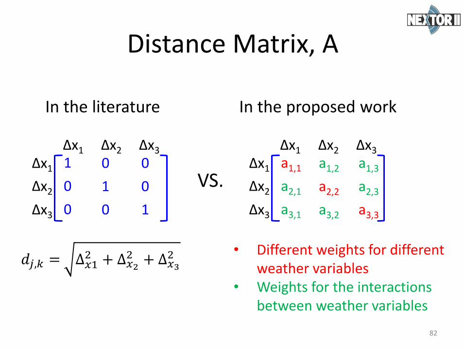
Distance Matrix, A
82
In the literature In the proposed work
∆x1 ∆x2 ∆x3
∆x1
∆x2
∆x3
1
0
0
0
1
0
0
0
1
∆x1 ∆x2 ∆x3
∆x1
∆x2
∆x3
a1,1
a2,1
a3,1
a1,2
a2,2
a3,2
a1,3
a2,3
a3,3
• Different weights for different weather variables
• Weights for the interactions between weather variables
𝑑𝑗,𝑘 = ∆𝑥1 + ∆𝑥2
+ ∆𝑥3
VS.

Recipe
83
S & D AHourly distances between WFs, 𝑑𝑖
timestart end
Given day
time
start end
Historical day𝑑1
1 2 n
1 2 n
𝑑 𝑑𝑛
Total distance between two days, σ𝑖=1
𝑛 𝑑𝑖
…
…
Extract capacity profiles from similar days with short total distances.These profiles are taken as planned capacity profiles

Topic 5: Benefit Mechanisms and User Grading Models
84
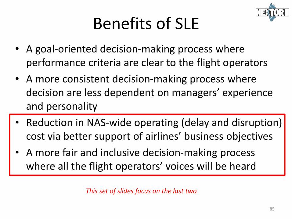
Benefits of SLE
• A goal-oriented decision-making process where performance criteria are clear to the flight operators
• A more consistent decision-making process where decision are less dependent on managers’ experience and personality
• Reduction in NAS-wide operating (delay and disruption) cost via better support of airlines’ business objectives
• A more fair and inclusive decision-making process where all the flight operators’ voices will be heard
85
This set of slides focus on the last two

Assessment Methods• CoUNSEL Design
– COuNSEL design is informed by assuming airlines vote according to the value functions computed by our modeling approach. (Aside from modeling approach, we also conducted a Human-In-The-Loop (HITL) experiment to get airline inputs)
• Benchmarks, compare COuNSEL design to
– Centralized (state-of-research) design: the design which has the least total aircraft delay cost (sum of ground delay and airborne delay cost) for all GDP-impacted incoming flights
– System-optimal design: the design which has the least total delay and disruption cost (both aircraft and passenger delay/disruption) by summing over the delay cost of each airline. This approach accounts for airline recovery actions.
• Notes
– FAA traffic managers make decisions in designing GDPs and these decisions impact airlines’ operating bottom lines. COuNSEL design most likely will not necessarily lead to an improvement in traditional system performance metrics, e.g. overall throughput or delay. Rather it will lead to a better economic performance for the airlines and fairer distribution of outcomes among different airlines.
86
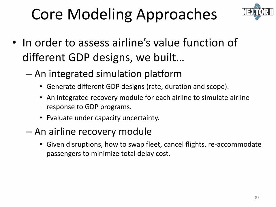
Core Modeling Approaches
• In order to assess airline’s value function of different GDP designs, we built…
– An integrated simulation platform • Generate different GDP designs (rate, duration and scope).
• An integrated recovery module for each airline to simulate airline response to GDP programs.
• Evaluate under capacity uncertainty.
– An airline recovery module • Given disruptions, how to swap fleet, cancel flights, re-accommodate
passengers to minimize total delay cost.
87
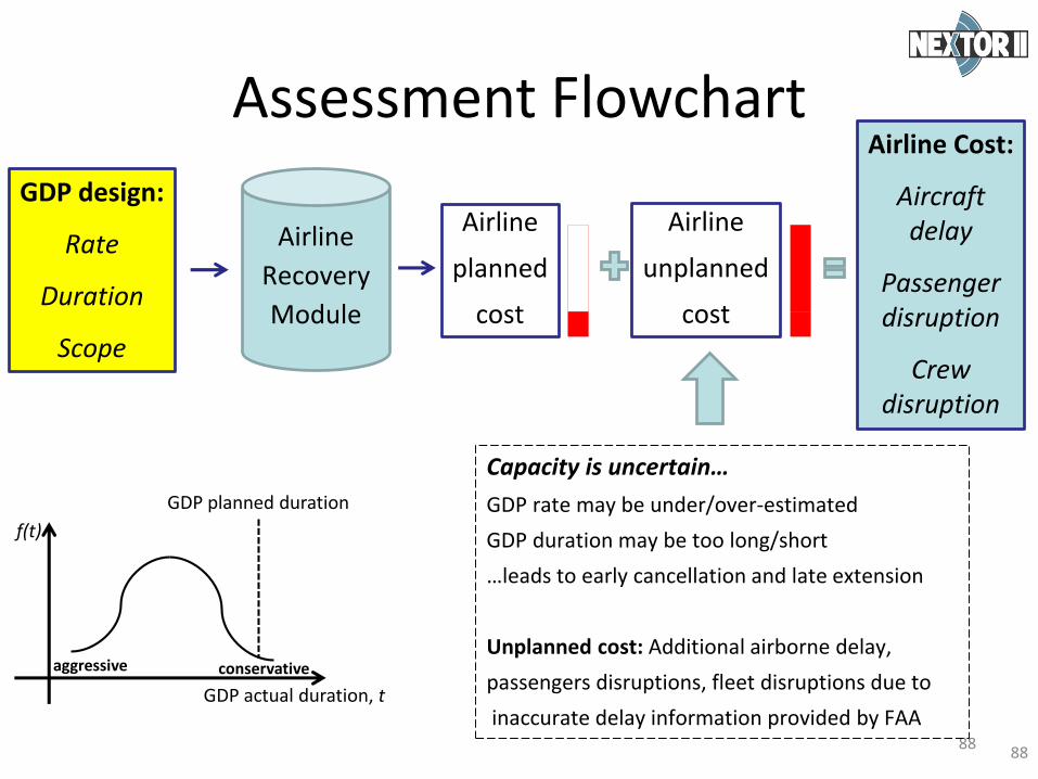
Assessment Flowchart
8888
GDP design:
Rate
Duration
Scope
Airline Cost:
Aircraft delay
Passenger disruption
Crew disruption
Airline
Recovery
Module
Airline
planned
cost
Airline
unplanned
cost
GDP actual duration, t
f(t)
GDP planned duration
conservativeaggressive
Capacity is uncertain…
GDP rate may be under/over-estimated
GDP duration may be too long/short
…leads to early cancellation and late extension
Unplanned cost: Additional airborne delay,
passengers disruptions, fleet disruptions due to
inaccurate delay information provided by FAA
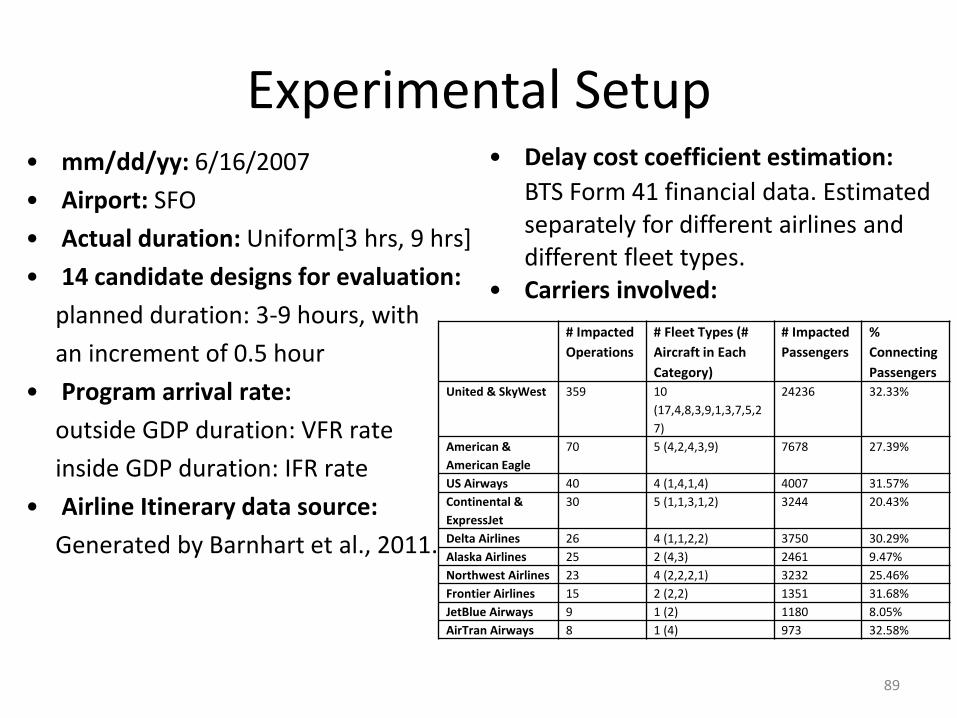
Experimental Setup
89
• mm/dd/yy: 6/16/2007
• Airport: SFO
• Actual duration: Uniform[3 hrs, 9 hrs]
• 14 candidate designs for evaluation:
planned duration: 3-9 hours, with
an increment of 0.5 hour
• Program arrival rate:
outside GDP duration: VFR rate
inside GDP duration: IFR rate
• Airline Itinerary data source:
Generated by Barnhart et al., 2011.
• Delay cost coefficient estimation:
BTS Form 41 financial data. Estimated separately for different airlines and different fleet types.
• Carriers involved:
# Impacted
Operations
# Fleet Types (#
Aircraft in Each
Category)
# Impacted
Passengers
%
Connecting
Passengers
United & SkyWest 359 10
(17,4,8,3,9,1,3,7,5,2
7)
24236 32.33%
American &
American Eagle
70 5 (4,2,4,3,9) 7678 27.39%
US Airways 40 4 (1,4,1,4) 4007 31.57%
Continental &
ExpressJet
30 5 (1,1,3,1,2) 3244 20.43%
Delta Airlines 26 4 (1,1,2,2) 3750 30.29%
Alaska Airlines 25 2 (4,3) 2461 9.47%
Northwest Airlines 23 4 (2,2,2,1) 3232 25.46%
Frontier Airlines 15 2 (2,2) 1351 31.68%
JetBlue Airways 9 1 (2) 1180 8.05%
AirTran Airways 8 1 (4) 973 32.58%

Revealing Airline’s Preference
90
Airline # Impacted
Operations
# Fleet Types (# Aircraft in
Each Category)
# Impacted
Passengers
% Connecting
Passengers
Average Load
Factor
US Airways 40 4 (1,4,1,4) 4007 31.57% 80.43%
-40000
-20000
0
20000
40000
60000
80000
100000
120000
140000
3 3.5 4 4.5 5 5.5 6 6.5 7 7.5 8 8.5 9 9.5
Tota
l C
ost
($)
Aggressive ← GDP Planned Duration (hours) → Conservative
Total Realized Cost
Total Realized Cost (no recovery)
Planned Total Cost
Unplanned Total Cost
total cost trend: preference for aggressive design (shorter planned duration)
small number of total operations, multiple different fleet type
little flexibility for recovery(reduces 6.6% cost through recovery at most)

Revealing Airline’s Preference
91
Airline # Impacted
Operations
# Fleet Types (# Aircraft in
Each Category)
# Impacted
Passengers
% Connecting
Passengers
Average Load
Factor
American &
American Eagle
70 5 (4,2,4,3,9) 7678 27.39% 75.53%
-50000
0
50000
100000
150000
200000
250000
3 3.5 4 4.5 5 5.5 6 6.5 7 7.5 8 8.5 9 9.5
Tota
l C
ost
($)
Aggressive ← GDP Planned Duration (hours) → Conservative
Total Realized Cost
Total Realized Cost (no recovery)
Planned Total Cost
Unplanned Total Cost
total cost trend: preference for moderate design (intermediate planned duration)
medium number of total operations, multiple different fleet type
medium flexibility for recovery (reduces 32.4% cost through recovery at most)

Revealing Airline’s Preference
92
Airline # Impacted
Operations
# Fleet Types (# Aircraft in
Each Category)
# Impacted
Passengers
% Connecting
Passengers
Average Load
Factor
United & SkyWest 359 10 (17,4,8,3,9,1,3,7,5,27) 24236 32.33% 75.29%
-200000
-100000
0
100000
200000
300000
400000
500000
600000
700000
800000
900000
3 3.5 4 4.5 5 5.5 6 6.5 7 7.5 8 8.5 9 9.5
Tota
l C
ost
($)
Aggressive ← GDP Planned Duration (hours) → Conservative
Total Realized Cost
Total Realized Cost (no recovery)
Planned Total Cost
Unplanned Total Cost
total cost trend: preference for conservative design (longer planned duration)
extremely large number of total operations, multiple different fleet type
great flexibility for recovery(reduces 62.3% cost through recovery at most)
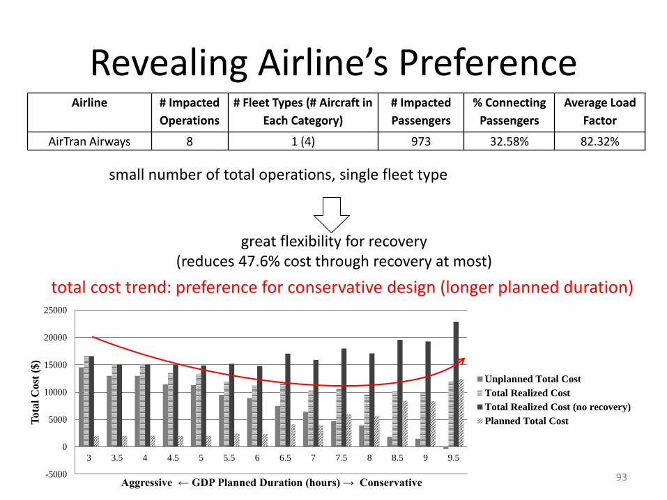
Revealing Airline’s Preference
93
Airline # Impacted
Operations
# Fleet Types (# Aircraft in
Each Category)
# Impacted
Passengers
% Connecting
Passengers
Average Load
Factor
AirTran Airways 8 1 (4) 973 32.58% 82.32%
-5000
0
5000
10000
15000
20000
25000
3 3.5 4 4.5 5 5.5 6 6.5 7 7.5 8 8.5 9 9.5
Tota
l C
ost
($)
Aggressive ← GDP Planned Duration (hours) → Conservative
Unplanned Total Cost
Total Realized Cost
Total Realized Cost (no recovery)
Planned Total Cost
total cost trend: preference for conservative design (longer planned duration)
small number of total operations, single fleet type
great flexibility for recovery(reduces 47.6% cost through recovery at most)
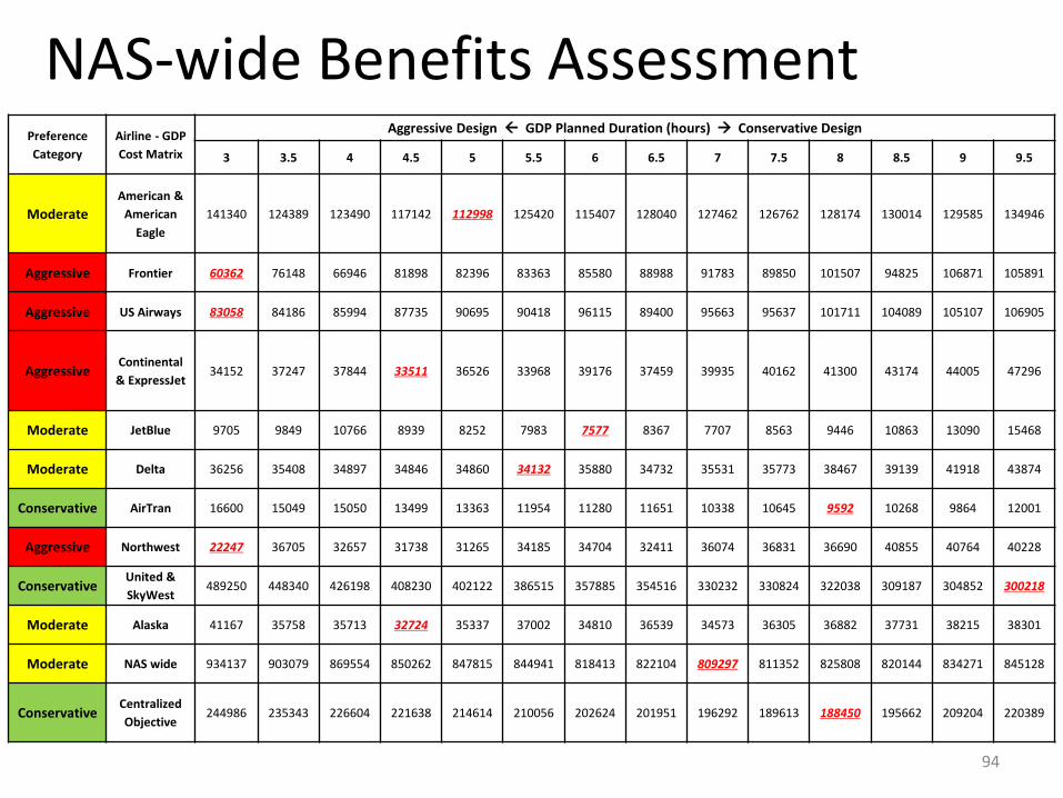
NAS-wide Benefits Assessment
94
Preference
Category
Airline - GDP
Cost Matrix
Aggressive Design GDP Planned Duration (hours) Conservative Design
3 3.5 4 4.5 5 5.5 6 6.5 7 7.5 8 8.5 9 9.5
Moderate
American &
American
Eagle
141340 124389 123490 117142 112998 125420 115407 128040 127462 126762 128174 130014 129585 134946
Aggressive Frontier 60362 76148 66946 81898 82396 83363 85580 88988 91783 89850 101507 94825 106871 105891
Aggressive US Airways 83058 84186 85994 87735 90695 90418 96115 89400 95663 95637 101711 104089 105107 106905
AggressiveContinental
& ExpressJet34152 37247 37844 33511 36526 33968 39176 37459 39935 40162 41300 43174 44005 47296
Moderate JetBlue 9705 9849 10766 8939 8252 7983 7577 8367 7707 8563 9446 10863 13090 15468
Moderate Delta 36256 35408 34897 34846 34860 34132 35880 34732 35531 35773 38467 39139 41918 43874
Conservative AirTran 16600 15049 15050 13499 13363 11954 11280 11651 10338 10645 9592 10268 9864 12001
Aggressive Northwest 22247 36705 32657 31738 31265 34185 34704 32411 36074 36831 36690 40855 40764 40228
ConservativeUnited &
SkyWest489250 448340 426198 408230 402122 386515 357885 354516 330232 330824 322038 309187 304852 300218
Moderate Alaska 41167 35758 35713 32724 35337 37002 34810 36539 34573 36305 36882 37731 38215 38301
Moderate NAS wide 934137 903079 869554 850262 847815 844941 818413 822104 809297 811352 825808 820144 834271 845128
ConservativeCentralized
Objective244986 235343 226604 221638 214614 210056 202624 201951 196292 189613 188450 195662 209204 220389

NAS-wide Benefits Assessment
95
Airline - GDP
Grade Matrix
# impacted
operationweights
Aggressive Design GDP Planned Duration (hours) Conservative Design
3 3.5 4 4.5 5 5.5 6 6.5 7 7.5 8 8.5 9 9.5
American &
American
Eagle
70 17.97 80 91 92 96 100 90 98 88 89 89 88 87 87 84
Frontier 15 6.30 100 79 90 74 73 72 71 68 66 67 59 64 56 57
US Airways 40 12.28 100 99 97 95 92 92 86 93 87 87 82 80 79 78
Continental
& ExpressJet30 10.1 98 90 89 100 92 99 86 89 84 83 81 78 76 71
JetBlue 9 4.45 78 77 70 85 92 95 100 91 98 88 80 70 58 49
Delta 26 9.16 94 96 98 98 98 100 95 98 96 95 89 87 81 78
AirTran 8 4.11 58 64 64 71 72 80 85 82 93 90 100 93 97 80
Northwest 23 8.43 100 61 68 70 71 65 64 69 62 60 61 54 55 55
United &
SkyWest359 54.63 61 67 70 74 75 78 84 85 91 91 93 97 98 100
Alaska 25 8.92 79 92 92 100 93 88 94 90 95 90 89 87 86 85
Majority judgement winner coincides with system-optimal design!!
Linearly transform costs into 100-scale grades…

NAS-wide Benefits Assessment
96
800000
820000
840000
860000
880000
900000
920000
940000
960000
0
50000
100000
150000
200000
250000
300000
2.5 3 3.5 4 4.5 5 5.5 6 6.5 7 7.5 8 8.5 9 9.5 10
NA
S-w
ide
Tota
l C
ost
($)
Cen
trail
ized
Ob
ject
ive
Valu
e ($
)
Aggressive ← GDP Planned Duration (hours) → Conservative
Centralized Design, System Optimal Design, COuNSEL Design and Historical Design
Centralized objective value
NAS-wide total cost
centralizeddesign
COuNSELdesign
(system-optimal)
historicaldesign
To centralized design:COuNSEL reduces2.0% in NAS-widetotal cost
To historical design:COuNSEL reduces4.2% in NAS-widetotal cost
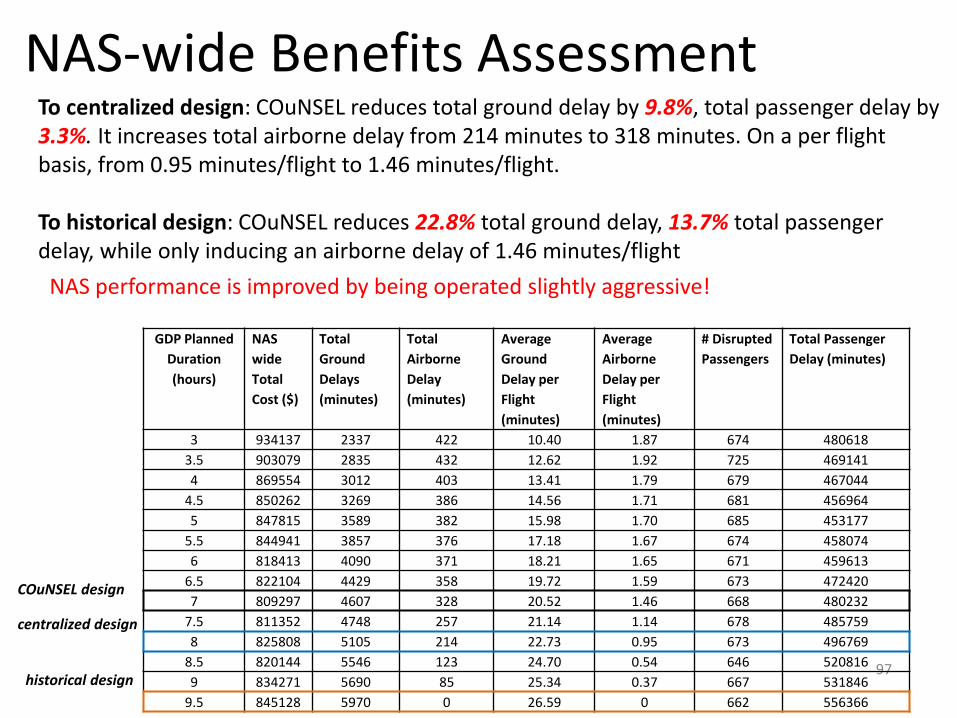
NAS-wide Benefits Assessment
97
GDP Planned
Duration
(hours)
NAS
wide
Total
Cost ($)
Total
Ground
Delays
(minutes)
Total
Airborne
Delay
(minutes)
Average
Ground
Delay per
Flight
(minutes)
Average
Airborne
Delay per
Flight
(minutes)
# Disrupted
Passengers
Total Passenger
Delay (minutes)
3 934137 2337 422 10.40 1.87 674 480618
3.5 903079 2835 432 12.62 1.92 725 469141
4 869554 3012 403 13.41 1.79 679 467044
4.5 850262 3269 386 14.56 1.71 681 456964
5 847815 3589 382 15.98 1.70 685 453177
5.5 844941 3857 376 17.18 1.67 674 458074
6 818413 4090 371 18.21 1.65 671 459613
6.5 822104 4429 358 19.72 1.59 673 472420
7 809297 4607 328 20.52 1.46 668 480232
7.5 811352 4748 257 21.14 1.14 678 485759
8 825808 5105 214 22.73 0.95 673 496769
8.5 820144 5546 123 24.70 0.54 646 520816
9 834271 5690 85 25.34 0.37 667 531846
9.5 845128 5970 0 26.59 0 662 556366
COuNSEL design
centralized design
historical design
To centralized design: COuNSEL reduces total ground delay by 9.8%, total passenger delay by 3.3%. It increases total airborne delay from 214 minutes to 318 minutes. On a per flight basis, from 0.95 minutes/flight to 1.46 minutes/flight.
To historical design: COuNSEL reduces 22.8% total ground delay, 13.7% total passenger delay, while only inducing an airborne delay of 1.46 minutes/flight
NAS performance is improved by being operated slightly aggressive!
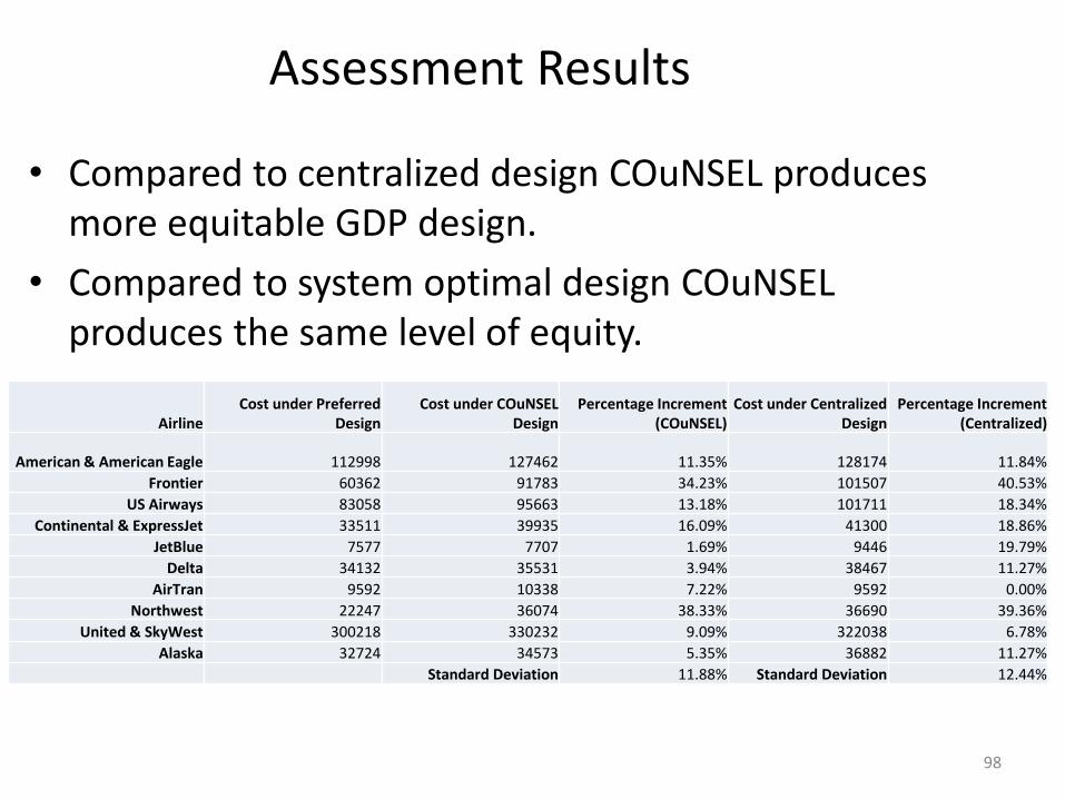
98
AirlineCost under Preferred
DesignCost under COuNSEL
DesignPercentage Increment
(COuNSEL)Cost under Centralized
DesignPercentage Increment
(Centralized)
American & American Eagle 112998 127462 11.35% 128174 11.84%
Frontier 60362 91783 34.23% 101507 40.53%
US Airways 83058 95663 13.18% 101711 18.34%
Continental & ExpressJet 33511 39935 16.09% 41300 18.86%
JetBlue 7577 7707 1.69% 9446 19.79%
Delta 34132 35531 3.94% 38467 11.27%
AirTran 9592 10338 7.22% 9592 0.00%
Northwest 22247 36074 38.33% 36690 39.36%
United & SkyWest 300218 330232 9.09% 322038 6.78%
Alaska 32724 34573 5.35% 36882 11.27%
Standard Deviation 11.88% Standard Deviation 12.44%
Assessment Results
• Compared to centralized design COuNSEL produces more equitable GDP design.
• Compared to system optimal design COuNSELproduces the same level of equity.

User Support Tools
99
• Various user support tools are developed to help airlines and FAA make corresponding decisions under SLE framework.
– SLE metrics tradeoff curves
– SLE metrics to TMI parameters mapping
– SLE metrics to airline performance mapping

User Support Tool #1: SLE Metric Tradeoff Curves
• Each slide gives four tradeoff curves showing the tradeoff between two SLE metrics for four values of the third SLE metric.

Efficiency vs Capacity Utilization Tradeoff
Eff vs CapUtilfor Pred =
.768
.803
.839
.874

Capacity Utilization vs Predictability
Tradeoff
CapUtil vs Predfor Eff =
.366
.576
.785
.994
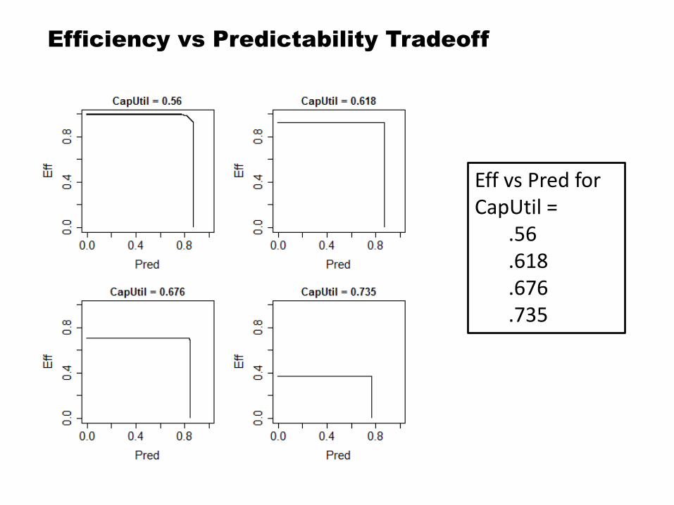
Efficiency vs Predictability Tradeoff
Eff vs Pred for CapUtil =
.56
.618
.676
.735

User Support Tool #2: SLE Vectors to TMI Parameters
Mapping
• For the FAA traffic managers and for each scenario a mapping is given from a set of SLE metric vectors to corresponding TMI plans/parameters.

Goal Vectors to TMI Parameters Mapping(Use GDP as an example)
• Goals: capacity utilization, efficiency, predictability• GDP parameters: start time, end time, planned called rates
Goal vectorsTMI parameters
Planned start time
planned end time
Called rates(arrivals per quarter hour)
Capacity utilization Efficiency Predictability 11:00-11:15 11:15-11:30 11:30-11:45 … 22:45-23:00
0.651 0.839 0.869 11:15:00 0:45:00 8 8 8 … 8
0.614 0.894 0.836 13:04:00 1:31:40 10 10 9 … 7
0.668 0.665 0.854 13:05:00 0:23:20 9 9 8 … 8
0.617 0.934 0.875 11:30:00 1:26:40 8 8 8 … 8
0.615 0.927 0.880 11:15:00 1:28:07 8 8 8 … 8
0.582 0.982 0.822 11:15:00 2:18:45 8 8 8 … 8
0.647 0.770 0.843 12:56:00 0:25:30 9 9 9 … 9
0.560 0.994 0.769 10:30:00 3:01:52 8 7 7 … 7
0.735 0.349 0.765 13:37:00 22:06:00 10 13 13 … 9
0.610 0.943 0.867 11:45:00 1:35:37 9 9 8 … 8
0.718 0.471 0.795 13:20:00 22:36:40 10 10 9 … 9
0.671 0.629 0.840 11:15:00 0:16:52 8 8 8 … 8
0.617 0.918 0.873 12:20:00 1:25:00 9 9 8 … 8
0.658 0.777 0.865 11:45:00 0:36:00 9 9 8 … 8

User Support Tool #3: SLE Vectors to User Performance
Indicator Mapping
• For each flight operator and for each scenario a mapping is given from a sample of SLE metric vectors to user performance indicators.
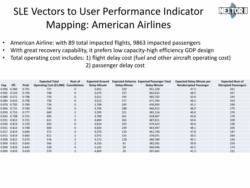
SLE Vectors to User Performance Indicator Mapping: American Airlines
• American Airline: with 89 total impacted flights, 9863 impacted passengers• With great recovery capability, it prefers low capacity-high efficiency GDP design• Total operating cost includes: 1) flight delay cost (fuel and other aircraft operating cost)
2) passenger delay cost
Cap. Eff. Pred.Expected Total
Operating Cost ($1,000)Num of
CancellationsExpected Ground
Delay MinuteExpected Airborne
Delay MinuteExpected Passenger Total
Delay MinuteExpected Delay Minute per
Nondisrupted PassengerExpected Num of
Disrupted Passengers0.996 0.484 0.791 727 0 2,852 320 451,228 47.3 2610.992 0.529 0.796 748 0 3,073 337 462,632 48.5 2670.989 0.571 0.798 754 0 3,011 345 485,702 50.8 2450.984 0.610 0.798 730 0 3,013 217 471,783 49.4 2540.970 0.705 0.789 726 0 3,708 295 430,993 45.2 2900.964 0.731 0.784 744 0 3,794 288 466,915 48.9 2750.959 0.753 0.777 669 2 3,395 221 382,214 40.0 2760.942 0.798 0.752 695 2 3,780 261 418,667 43.8 2700.931 0.812 0.731 621 0 4,869 265 487,811 50.6 2090.926 0.814 0.720 603 0 4,810 255 479,422 49.6 1900.921 0.813 0.708 600 0 4,820 239 463,497 48.1 2050.917 0.814 0.696 571 0 4,970 120 461,740 47.8 1870.912 0.814 0.683 611 2 3,972 155 379,071 39.5 2640.908 0.815 0.670 576 2 4,273 128 386,789 40.1 2260.904 0.815 0.656 566 2 4,250 91 382,581 39.8 2500.900 0.816 0.643 528 0 5,102 50 440,946 45.5 1740.899 0.816 0.639 570 2 4,809 20 397,665 41.3 231
Conclusion
116
• In most of the cases, COuNSEL has the capability to reduce system-wide total delay cost, and produce more equitable design.
• COuNSEL leads to a better economic performance for the airlines and fairer distribution of outcomes among different airlines.

Topic 6: COuNSEL Software Tool
117
Software Tool
• Users are divided into administrators and participants
• Administrators create polls, approve submissions and can view detailed submission results
• Participants submit candidates, rank candidates and can view only the winning vector
118

Process
1. Administrator creates poll
2. Participants submit candidates
3. Administrator approves candidates and opens grading
4. Participants grade candidates
5. Results are shown
119
Necessary Inputs
• The following inputs will be required for each poll:
– User Accounts: each participants must have an account
– Group: participants are organized into groups
– Metric table: a table of constraints defining the feasible set of candidates
– Weight set: an assignment of weights to the participants
120

Groups
• Individuals are organized into groups
• When you make a poll, you need to create a group for that poll which contains the users that will vote in that poll
• Individuals may belong to more than one group
121

Metric Table
• The metric table is a list of constraints which describe the feasible set of candidates.
• These constraints take the form𝐴1 ∗ 𝑐𝑎 𝑎𝑐𝑖𝑡𝑦 + 𝐴 ∗ 𝑒𝑓𝑓𝑖𝑐𝑖𝑒𝑛𝑐𝑦 + 𝐴 ∗ 𝑟𝑒𝑑𝑖𝑐𝑡𝑎𝑏𝑖𝑙𝑖𝑡𝑦 ≤ 𝐵
where 𝐴1, 𝐴 , 𝐴 and B are all positive numbers.
• This tool requires that these numbers be at least 0.0001
122

Weight Sets
• Weight sets describe how much weight is given to each user during voting
• Weights can be any positive number with at most two decimal place
123

Candidate Format
• In the software, candidates are represented as a three dimensional vector:
𝑐𝑎 𝑎𝑐𝑖𝑡𝑦, 𝑒𝑓𝑓𝑖𝑐𝑖𝑒𝑛𝑐𝑦, 𝑟𝑒𝑑𝑖𝑐𝑡𝑎𝑏𝑖𝑙𝑖𝑡𝑦
• Each element of a candidate is usually represented as an integer percentage from 0 to 100
• Example: the candidate which achieves 50% capacity, 70% efficiency and 70% predictability is represented as
50,70,70
124

Candidate Format
• However, metric constraints are written in terms of decimal values instead of percentages
• Example: the constraint that the sum of the three metrics is no more than 200% for any candidate would be:
1 ∗ 𝑐𝑎 𝑎𝑐𝑖𝑡𝑦 + 1 ∗ 𝑒𝑓𝑓𝑖𝑐𝑖𝑒𝑛𝑐𝑦 + 1∗ 𝑟𝑒𝑑𝑖𝑐𝑡𝑎𝑏𝑖𝑙𝑖𝑡𝑦 ≤
125

Administrator Home Page
Create new polls
Active polls – participants are submitting candidates
Active polls - waiting for administrator to approve candidates
Active polls – participants are grading candidates
126

Administrator Home PageCompleted polls – can view results, or can create new polls based on the results of the completed poll
127

Participant home page
Active polls – participant may submit candidates
Active polls – participant may grade candidates
Results from completed polls are shown
128

Poll Creation - Administrator
The poll is given a name and description
We can create a table of metric constraints or choose an existing table 129
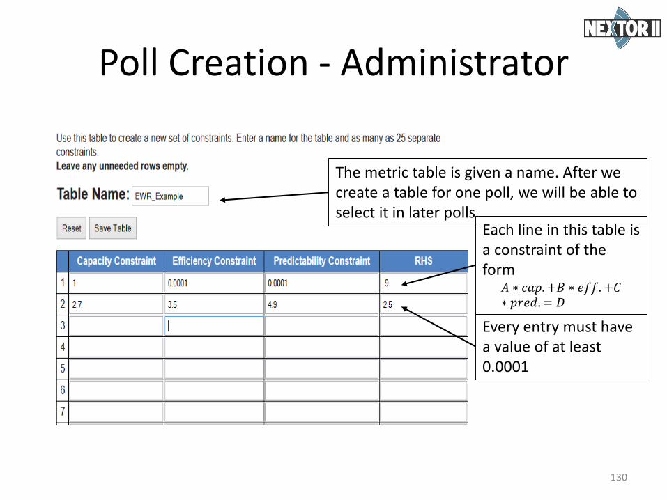
Poll Creation - Administrator
The metric table is given a name. After we create a table for one poll, we will be able to select it in later polls
Each line in this table is a constraint of the form
𝐴 ∗ 𝑐𝑎 . +𝐵 ∗ 𝑒𝑓𝑓. +𝐶∗ 𝑟𝑒𝑑. = 𝐷
Every entry must have a value of at least 0.0001
130
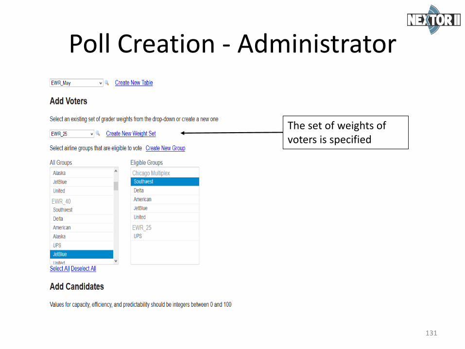
Poll Creation - Administrator
The set of weights of voters is specified
131
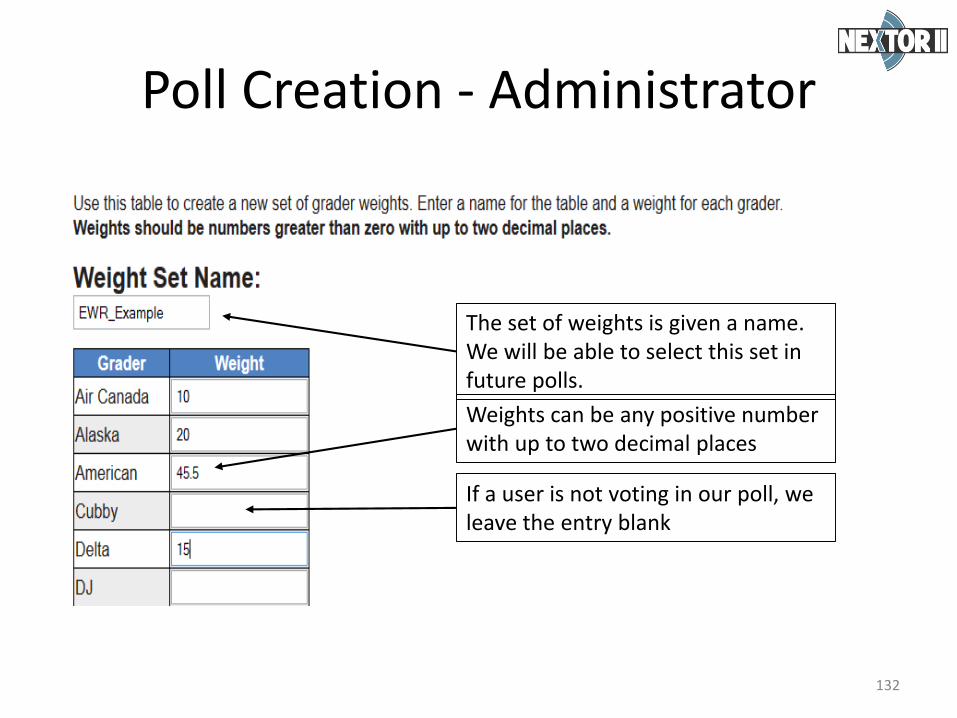
Poll Creation - Administrator
The set of weights is given a name. We will be able to select this set in future polls.
Weights can be any positive number with up to two decimal places
If a user is not voting in our poll, we leave the entry blank
132

Poll Creation - Administrator
We create a group of users for the poll or select an existing group
133

Poll Creation - Administrator
The group is given a name. We will be able to select this group in future polls.
We select which users will be able to participate in our poll
134

Poll Creation - AdministratorWe click on a group to add the users in that group to our poll.
Note: if an individual is in several groups, then they might be appear under a group other than the one we selected. This does not affect the functionality of the poll.We can also select individuals one at a time
Eligible users will appear in the “Eligible Groups” section
135

Poll Creation - AdministratorThe administrator can choose to submit some candidates for grading. These should be feasible, but the software allows infeasible ones.
Choose whether to also allow participants submit candidatesChoose how many candidates each user may submitChoose a time duration and then click the button to start accepting candidates
Each element of the candidate is an integer between 0-100
136

Candidate Submission - Participant
Third slider set automatically to highest feasible value
User uses sliders to set values of two parameters
Red color indicates that this slider was automatically set
137

Candidate approval - Administrator
Administrator may approve or reject any submitted candidate
138

Candidate approval - Administrator
Once the administrator has finished approving candidates, then the poll is opened to voting
139

Grading Candidates - Participants
Participants assign each candidate a grade using a slider
The rank that the user has given each candidate is shown
140
Viewing Results - Administrator
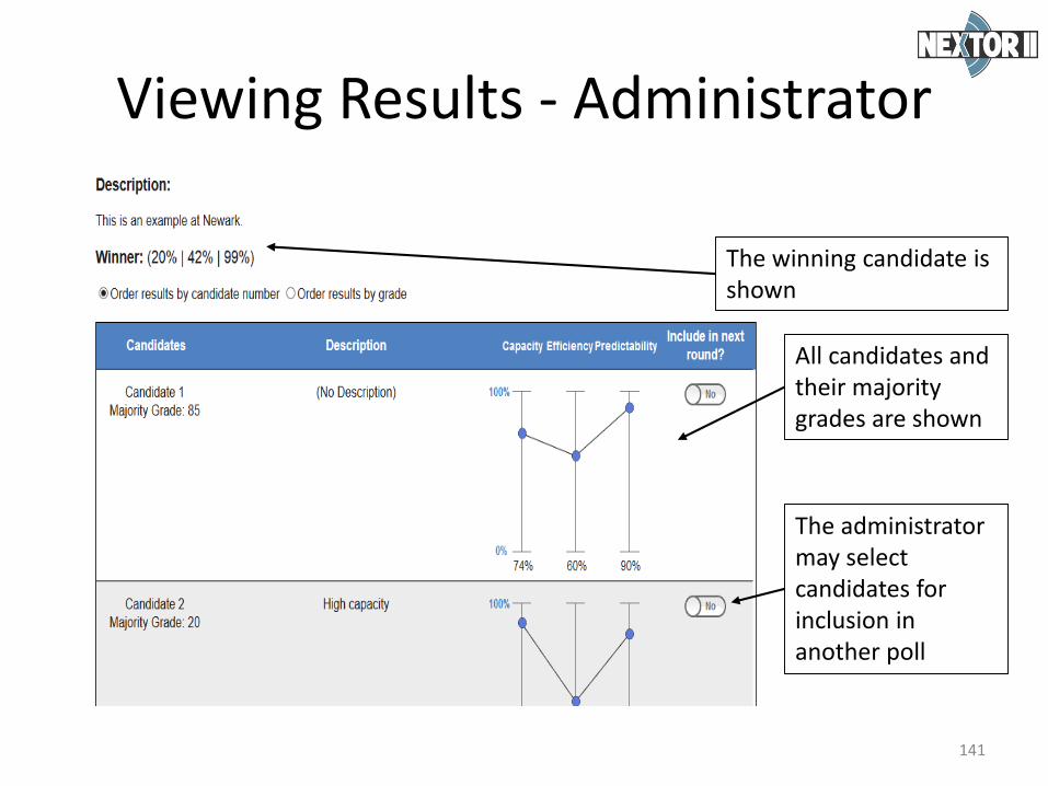
The winning candidate is shown
All candidates and their majority grades are shown
The administrator may select candidates for inclusion in another poll
141
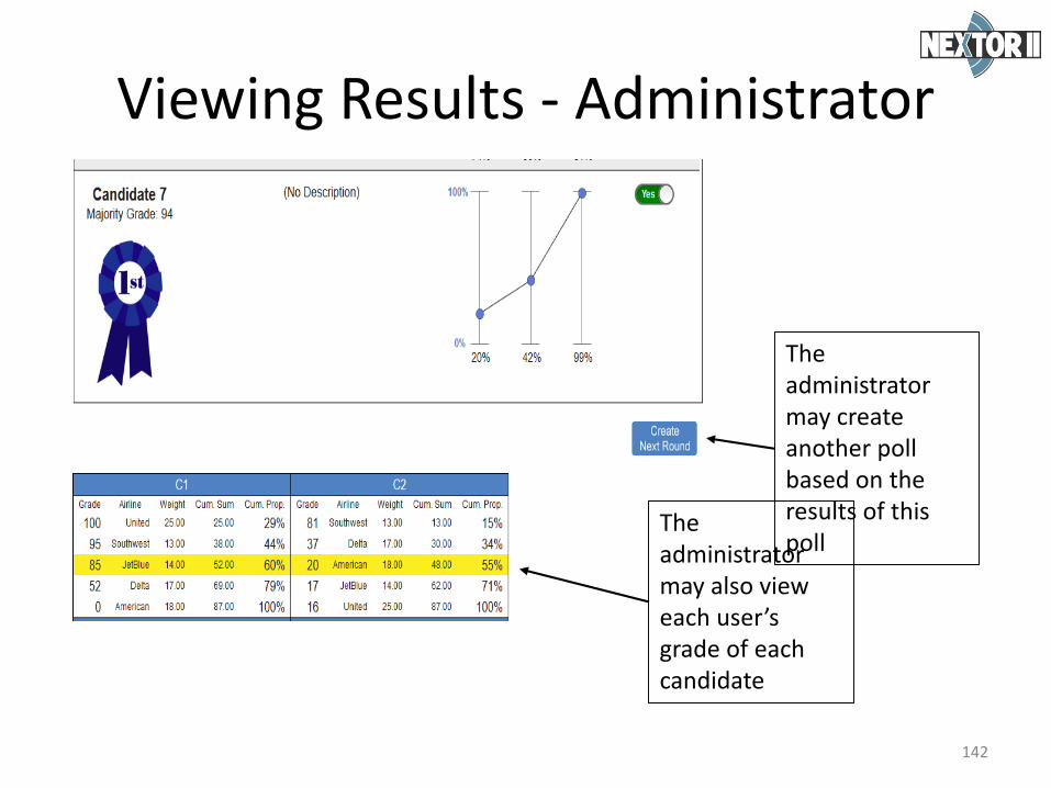
Viewing Results - Administrator
The administrator may also view each user’s grade of each candidate
The administrator may create another poll based on the results of this poll
142
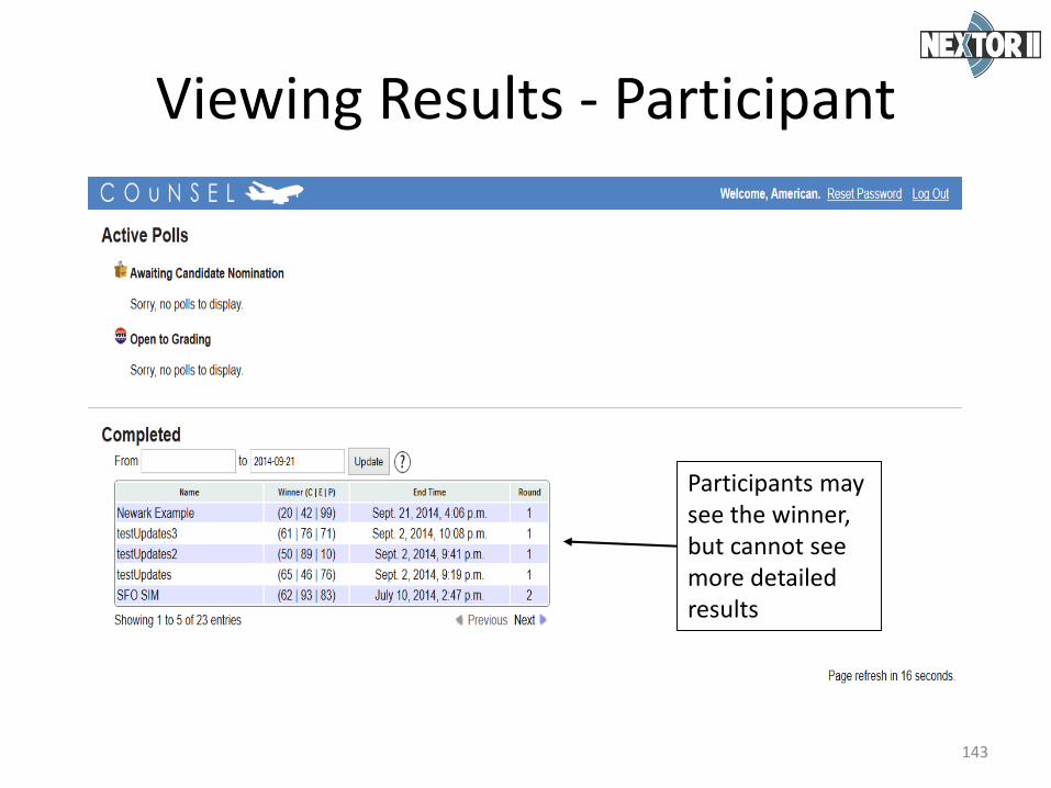
Viewing Results - Participant
Participants may see the winner, but cannot see more detailed results
143