SESAM Design and Characterization HOON JANG Master of Science Thesis Stockholm, Sweden 2010

SESAM Design and Characterization

HOON JANG

Master of Science Thesis

Laser Physics Department of Applied Physics School of Engineering Science

KTH

Stockholm, Sweden 2010

TRITA-FYS: 2010:16 ISSN: 0280-316X ISRN: KTH/FYS/- -10:16- -SE

ABSTRACT

This research is an essential preliminary work for building the compact ultrafast solid-state lasers using Semiconductor saturable absorber mirror (SESAM) devices and understanding its behaviour. In this work, I first built a reliable simulation tool to design SESAM devices so that we can tailor SESAM parameters suitable for building specific solid-state lasers. Secondly, I also built a SESAM characterization setup to measure its nonlinear saturation behavior, using the supercontinuum photonic crystal fiber (PCF) as a light source. For a demonstration of the setup, a commercial quantum well SESAM has been characterized, and the result will be presented. I will also discuss about the minimum output power and the stability of the light source required to improve the setup for a reliable parameter extraction.

ACKNOWLEDGEMENTS

This work was carried out at the laser physics group in KTH, where I had a very pleasant time while working and learning for my master thesis. There are some people whom I especially would like to thank. Prof. Valdas Pasiskevicius, whom I cannot thank enough for his guidance and support. Niels Meiser, thank you very much for all the helps in the experiments and revising my thesis even when you were very busy. Dr. Björn Jacobsson, thank you very much for the practical helps in the lab and the enlightening discussions. Nicky Thilmann, thank you very much for correcting small mistakes in my thesis. Dr. Mårten Stjernström, thank you very much for helping me find a reliable attenuator from the cell physics group in KTH. Andrius Zukauskas, Peter Rentschler, and Staffan Tjörnhammar, thank you for the emotional supports. I bully them time to time. Dr. Michael Fokine, and Patrik Holmberg, thank you very much for sharing the office with me, who seldom cleans the place. Prof. Jens Tellefsen, thank you very much for the kind supports, helping me solving a visa problem, for example. Last but not the least, thanks to prof. Fredrik Laurell, who is the most weird but awesome professor I have ever seen/met in the world. I am one of the people who are relying on his leadership and guidance.

Table of Contents

1. Introduction.................................................................................................................... 1

1.1 Background: why we need ultrafast lasers? 1.2 Ultrafast lasers and mode-locking methods in history 1.3 Purpose of this research: why we chose SESAMs? 1.4 Structure of this thesis

2. Mode-locking Techniques and Stability Condition.......................................................... 5

2.1 Mode-locking theory 2.2 Stable continuous-wave (cw) modelocking condition

3. Semiconductor Saturable Absorber Mirrors (SESAM)..................................................... 12

3.1 SESAM and its parameter 3.2 SESAM Design Criteria 3.3 Quantum Well (QW) SESAM vs. Quantum Dots (QD) SESAM

4. SESAM Structure Design.................................................................................................. 19

4.1 Transfer Matrix Method 4.2 Perturbation's point of view - resonant vs. antiresonant 4.3 Some examples - field structures, GDD, enhancement factors

4.3.1 Demonstration: LOFERS 4.3.2 Novel QD-SESAM structure 1 4.3.3 Novel QD-SESAM structure 2

5. Simulation of SESAM Saturation behaviour solving absorber rate equations............... 29

5.1 A simple model function for fitting measured data 5.2 Direct simulation

5.2.1 A slow absorber 5.2.2 A fast absorber

5.3 Self-Consistency 5.4 Quantum Dot Design?

6. Let There Be Light: Building and Characterizing a Light Source...................................... 37

6.1 Light source using FemtoWHITE CARS PCF Fiber 6.2 Spectroscopy and Data evaluation

6.2.1 Spectral Depletion and Special GVD curve 6.2.2 Autocorrelation measurement 6.2.3 Tunable Spectrum 6.2.4 Different SOP for different part of the spectrum 6.2.5 Instability of the output power and the output spectrum

7. SESAM Characterization.................................................................................................. 46

7.1 SESAM characterization setup 7.2 Alignment and calibration 7.3 Results and Discussion 7.4 Limitations

8. Conclusion and Future work........................................................................................... 57

Reference............................................................................................................................ 58

1

C h a p t e r 1

INTRODUCTION

1.1 Background: why do we need ultrafast lasers?

Ultrafast lasers are mode-locked lasers, which generate ultrashort pulses with durations of femtoseconds or picoseconds. The rapid developments in ultrafast laser technology over the past decades have been pushed by significant demands due to its important applications and benefits from its salient features such as ultrashort pulse duration, broad spectrum, and high peak intensity. Ultrashort pulse duration offers a high temporal resolution so that one can follow the dynamics of very fast events such as e.g. chemical reactions, and relaxation process of charge carriers in semiconductors. A broad spectrum enables a high spatial resolution for optical coherence tomography (OCT), which is a technique allowing high quality, 3D images in biological systems. A broadband frequency comb can be used as a ruler in a frequency domain so that one can measure unknown optical frequencies with a high spectral resolution. A high peak intensity is also very useful for an efficient nonlinear frequency conversion, and a ‘non-thermal’ ablation. Furthermore, a compact ultrafast laser can provide a high repetition rate (GHz) which can be used for a high capacity optical communication system.

1.2 Ultrafast lasers and mode-locking methods in history

Although there are several ways to achieve a pulsed laser operation by using the techniques such as Q-switching, cavity-dumping, or gain-switching, ultrafast lasers are almost always produced by a modelocking technique since it can generate much shorter pulses than other techniques. Basically, a modelocking is a technique to fix the phase relationship between the longitudinal modes in the laser cavity so that interference between them generates a train of extremely short pulses.

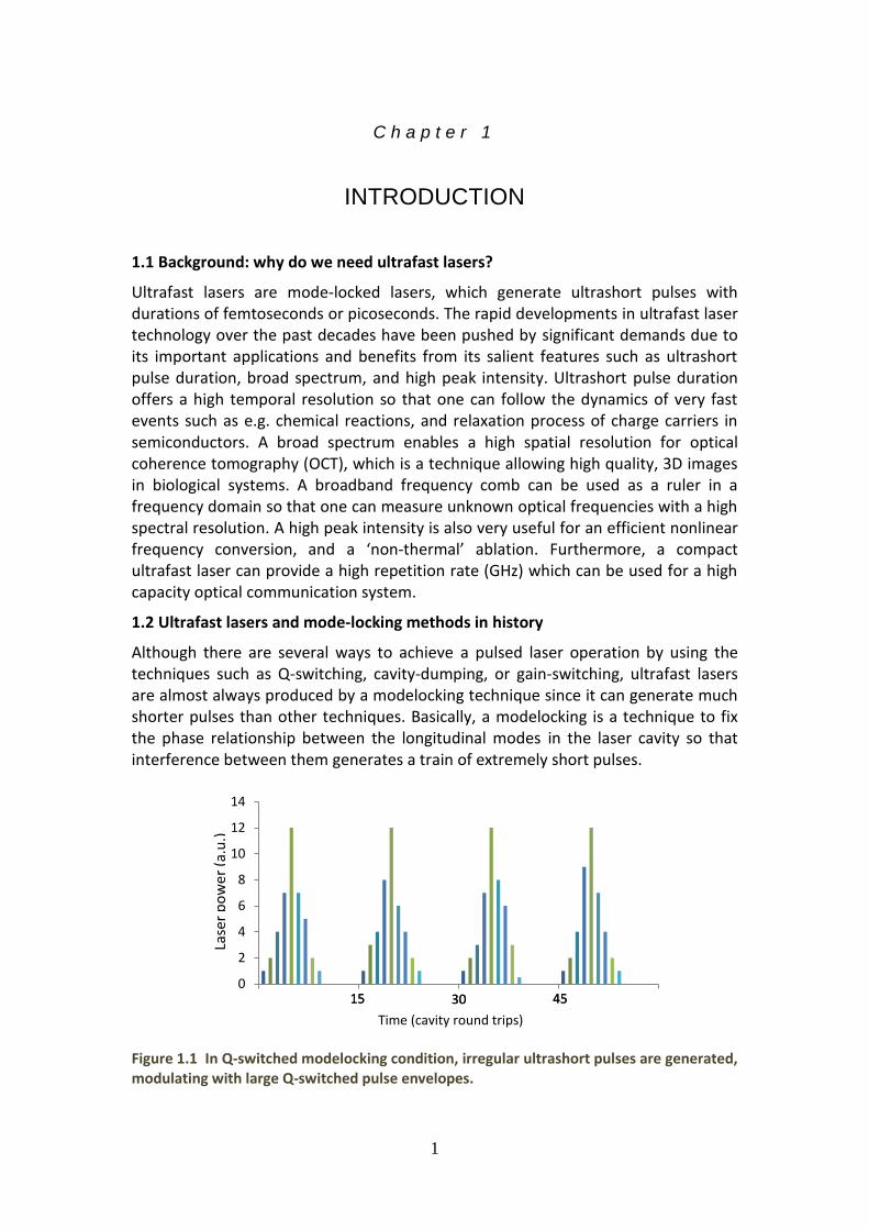
Figure 1.1 In Q-switched modelocking condition, irregular ultrashort pulses are generated, modulating with large Q-switched pulse envelopes.

0

2

4

6

8

10

12

14

Category 1 Category 2 Category 3 Category 4

Lase

rp

ow

er

(a.u

.)

Time (cavity round trips)

3015 45

Lase

rp

ow

er

(a.u

.)

Time (cavity round trips)

3015 45

2

Only 6 years after the very first laser was demonstrated, the first ultra short pulses were already produced using a passively modelocked Nd:glass laser [1]. The pulse was estimated to be few picoseconds long. But the pulse train was irregular, modulated with large Q-switched pulse envelopes. This phenomena is called Q-switched mode-locking (Fig.1.1).

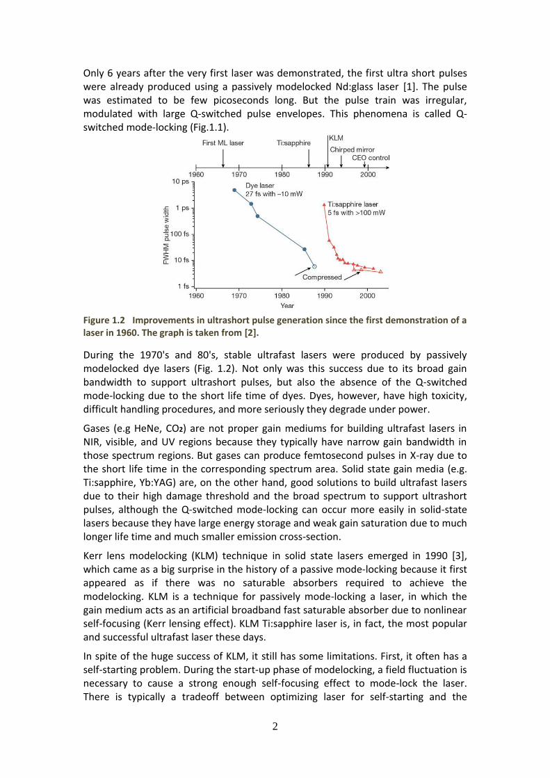
Figure 1.2 Improvements in ultrashort pulse generation since the first demonstration of a laser in 1960. The graph is taken from [2].

During the 1970's and 80's, stable ultrafast lasers were produced by passively modelocked dye lasers (Fig. 1.2). Not only was this success due to its broad gain bandwidth to support ultrashort pulses, but also the absence of the Q-switched mode-locking due to the short life time of dyes. Dyes, however, have high toxicity, difficult handling procedures, and more seriously they degrade under power.

Gases (e.g HeNe, CO2) are not proper gain mediums for building ultrafast lasers in NIR, visible, and UV regions because they typically have narrow gain bandwidth in those spectrum regions. But gases can produce femtosecond pulses in X-ray due to the short life time in the corresponding spectrum area. Solid state gain media (e.g. Ti:sapphire, Yb:YAG) are, on the other hand, good solutions to build ultrafast lasers due to their high damage threshold and the broad spectrum to support ultrashort pulses, although the Q-switched mode-locking can occur more easily in solid-state lasers because they have large energy storage and weak gain saturation due to much longer life time and much smaller emission cross-section.

Kerr lens modelocking (KLM) technique in solid state lasers emerged in 1990 [3], which came as a big surprise in the history of a passive mode-locking because it first appeared as if there was no saturable absorbers required to achieve the modelocking. KLM is a technique for passively mode-locking a laser, in which the gain medium acts as an artificial broadband fast saturable absorber due to nonlinear self-focusing (Kerr lensing effect). KLM Ti:sapphire laser is, in fact, the most popular and successful ultrafast laser these days.

In spite of the huge success of KLM, it still has some limitations. First, it often has a self-starting problem. During the start-up phase of modelocking, a field fluctuation is necessary to cause a strong enough self-focusing effect to mode-lock the laser. There is typically a tradeoff between optimizing laser for self-starting and the

3

shortest possible pulse length [4], since when the cavity is optimized for self-starting, KLM may saturate too much for ultrashort pulses, and the laser become unstable due to strong self-phase modulation (SPM). Secondly, the cavity design in KLM becomes harder for shorter cavities. As the cavity size becomes shorter, the repetition rate becomes higher and thus the peak power must become lower. Due to the lower peak power, one has to focus the beam harder so that the self-focusing effect becomes strong enough to achieve a mode-locking. Therefore, a cavity design in the KLM becomes more and more difficult as the cavity size becomes shorter and shorter for higher repetition rates. This difficulty is the most serious problem in KLM for building compact ultrafast lasers for high repetition rates. So, there has been a significant demand for alternative solutions for building compact ultrafast solid-state lasers. This is where a SESAM comes into the play.

Semiconductor saturable absorber mirrors (SESAMs, see Chapter 3) enable independent cavity designs and a wide range of tunable absorber parameters, which are in contrast to the limitations in KLM. It was a minor revolution in 1992 that a solid-state laser (Nd:YLF) was passively mode-locked [2, 5] using SESAMs to produce regular pulse trains, i.e. without Q-switched envelopes. Since the Q-switched mode-locking can occur more easily in solid-state lasers with long upper level lifetime, a wide range of tunable absorber parameters is very helpful to satisfy the stability condition against QML (see Chapter 2). This is possible using SESAMs.

1.3 Purpose of this research: why do we choose SESAMs? First of all, since solid-state lasers are operating with weak gain saturation, the absorber parameters have to be carefully adapted to satisfy the stability condition against Q-switched modelocking (see Chapter 2). Control of the parameters such as modulation depth, saturation fluence, and even the group delay dispersion (GDD) is possible by using SESAMs. Second, the impulse response in semiconductor is intrinsically bi-exponential due to intraband thermalization and interband recombination. The latter is much slower than the former by orders of magnitude. The faster response is important for stabilizing ultrashort pulses, while the slower response is also practically important for self-starting. Third, SESAM enables to use absorber characteristics as independent parameters in mode-locked laser cavity design. Thus SESAMs become more attractive for building compact ultrafast lasers. In KLM, on the other hand, a cavity design becomes more and more difficult as the cavity size becomes shorter because the beam has to be focused harder to increase the self-focusing effect.

Limitations of a SESAMs, however, lie in its damage threshold and the shortest possible pulse length due to a dispersion. The damage threshold of semiconductor material is significantly lower than the solid state gain medium, e.g. Ti:sapphire. Furthermore, the low dispersion band of SESAM is not as broad as that of KLM. Thus, SESAM is not favored in the generation of few-cycle pulses.

4

This research is an essential preliminary work for building the compact ultrafast solid-state lasers modelocked with a SESAM device. In this work, I first built a reliable simulation tool to design the SESAM devices so that we can tailor the SESAM parameters suitable for building specific solid-state lasers including e.g. fiber lasers. Secondly, I have also built a SESAMs characterization setup to measure the nonlinear saturation behavior with the supercontinuum photonic crystal fiber (PCF) used as a light source.

1.4 Structure of this thesis Chapter 2, I will start with introducing modelocking techniques, and fully derive the stability condition in detail for a cw mode-locked laser. Focusing on SESAMs in Chapter 3, I will explain their parameters and design criteria in details. Chapter 4 will show the SESAM design capability by simulating the field structures, group-delay dispersion (GDD), and linear reflectivity spectrum, using the transfer-matrix method. Based on the simulation in Chapter 4, the SESAMs saturation behaviour is calculated in Chapter 5 by solving the absorber rate equations. In Chapter 6, the physical phenomenon of a dramatic change of spectrum in photonic crystal fibers (PCF) will be studied. The PCF is experimentally characterized by measuring the output spectrum and the pulse width. In Chapter 7, the SESAM characterization setup I built will be presented, followed by the experimental results showing the nonlinear reflectivity of the SESAM. Lastly, in Chapter 8, I will briefly summarize the thesis with conclusions and propose the future works.

5

C h a p t e r 2

MODE-LOCKING THEORY

AND STABILITY CONDITION

2.1 Mode-locking theory When a laser is oscillating with a number of longitudinal modes, the phase of each mode may have a random value. Interference terms of these modes will be canceled out due to their random phases, and the laser will exhibit continuous-wave operation if there is no additional technique applied to generate pulses. If we manage to keep the interference terms by fixing the phases of the modes, one can imagine that we will have an intensity modulation as an interference, which is equivalent to a train of pulses in the time domain via simple Fourier transformation. Simply put, modelocking is the technique to fix phase relationship among the longitudinal modes of the laser cavity so that interference between them generates a train of short pulses.

Mode locking methods can be divided into two classes: active and passive. In active mode locking, some external source is used to drive the mode locking element, while in passive mode locking a saturable absorber is commonly used. The latter can generate much shorter pulses because a response of external sources can hardly be so sharp as that of saturable absorbers in passive mode locking. I will focus on passive mode-locked solid-state lasers, which is of our interest in this thesis.

Even though the basic idea of mode locking is simply an interference, i.e. a sum of the field vectors of a number of different modes, the dynamics of ultrashort pulse is usually much more complicated because it involves e.g. dispersion, self-phase modulation (SPM), and the gain filtering effects. For a stable mode locking, the average dynamics of the pulse is governed by Haus' master equation [6], which is actually a version of Ginzburg Landau equation adapted by Haus as follow:

𝑇𝑅

𝜕

𝜕𝑇𝐴 𝑇, 𝑡 = −𝑖𝐷

𝜕2

𝜕𝑡2+ 𝑖𝛿 𝐴 2 𝐴

+ 𝑔(𝑇, 𝑡) − 𝑙 + 𝐷𝑔 ,𝑓

𝜕2

𝜕𝑡2− 𝑞(𝑇, 𝑡) 𝐴

(2.1)

where 𝐴 𝑇, 𝑡 is the field with slowly varying envelope approximation (SVEA), 𝑇𝑅 the

cavity round-trip time, D the intracavity GDD, 𝐷𝑔 ,𝑓 = 𝑔 Ω𝑔2 the gain dispersion with

bandwidth (Ω𝑔) at HWHM, 𝛿 the SPM coefficient, and 𝑙 the round-trip losses. 𝑔 and

𝑞 denote the saturable gain and absorption, respectively. Note that we distinguish 𝑡 and 𝑇 in such a way that 𝑡 is the actual time scale in the lab, and 𝑇 = 𝑛𝑇𝑅 is a coarse-grained time scale to describe the pulse-to-pulse dynamics in the cavity.

As long as the behaviour of the absorber and the gain medium is based on the population difference like in two-level systems, they can be described by general rate equations:

6

𝑑𝑞(𝑇, 𝑡)

𝑑𝑡= −

𝑞 − 𝑞0

𝜏𝐴−

𝑃

𝐸𝑠𝑎𝑡 ,𝐴𝑞 (2.2)

𝑑𝑔(𝑇, 𝑡)

𝑑𝑡= −

𝑔 − 𝑔0

𝜏𝐿−

𝑃

𝐸𝑠𝑎𝑡 ,𝐿𝑔 (2.3)

These equations (2.1), (2.2) and (2.3) can provide a concrete model for the mode-locked lasers.

2.2 Stable continuous-wave modelocking condition

Simplified analytical formulations of cw modelocking condition has been developed in several papers (e.g. [7] [8]). The derivations, however, in those theoretical papers are not fully shown in details, we should not believe them until we see how they have been derived. Thus, I will give the full derivation of the stability condition for continuous-wave (cw) modelocking in solid state lasers.

To see the average dynamics of the pulse in a cavity, we should first know the average saturation behavior of an absorber and the gain in the coarse-grained time scale 𝑇 = 𝑛𝑇𝑅 . I will start with a slow absorber first, and go on to the gain rate equation and the cavity rate equation which are two coupled differential equations. By solving the two coupled rate equations for a relaxation oscillation, one can obtain the stability condition for cw modelocking.

Absorber saturation behavior

For slow absorbers, we may neglect the first term in Eq.(2.2) and integrate,

𝑑𝑞

𝑞= −

1

𝐸𝑠𝑎𝑡 ,𝐴 𝑃𝑑𝑡

and then we obtain the saturation behavior:

𝑞(𝑇, 𝑡) = 𝑞0𝑒𝑥𝑝 −𝐸(𝑡)

𝐸𝑠𝑎𝑡 ,𝐴

= 𝑞0𝑒𝑥𝑝 −𝐸𝑃(𝑇)

𝐸𝑠𝑎𝑡 ,𝐴 𝑓 𝑡′ 𝑑𝑡′

𝑡

−𝑇𝑅/2

where 𝑓 𝑡 𝑑𝑡 = 1

𝑇𝑅/2

−𝑇𝑅/2. (2.4)

Thus, the loss in pulse energy due to the absorber per single round trip can be written as:

𝑞𝑃 𝑇 = 𝑓 𝑡 𝑞 𝑇, 𝑡

𝑇𝑅2

−𝑇𝑅2

𝑑𝑡 = −𝐸𝑠𝑎𝑡 ,𝐴

𝐸𝑃(𝑇) 𝑞(𝑇, 𝑡) −𝑇𝑅/2

𝑇𝑅/2

= 𝑞0

𝐸𝑠𝑎𝑡 ,𝐴

𝐸𝑃 1 − 𝑒𝑥𝑝 −

𝐸𝑃(𝑇)

𝐸𝑠𝑎𝑡 ,𝐴

(2.5)

Even though the Eq.(2.5) was derived for slow absorbers, it has been reported that final result will stay valid even for the absorbers of which the relaxation time is as short as the pulse duration [7].

7

Gain rate equation

Regarding the saturation behavior of gain medium, we can readily average Eq.(2.3) over one round trip, because the gain saturation within one pulse is negligible in solid state lasers due to its small emission cross section that is typically more than 1,000 times smaller than other sort of gain material such as dyes or semiconductors. Thus, after averaging Eq.(2.3), we obtain:

𝑑𝑔

𝑑𝑇= −

𝑔 − 𝑔0

𝜏𝐿−

𝑃𝑎𝑣𝑔

𝐸𝑠𝑎𝑡 ,𝐿𝑔 = −

𝑔 − 𝑔0

𝜏𝐿−

𝐸𝑃

𝐸𝑠𝑎𝑡 ,𝐿𝑇𝑅𝑔

(2.6)

Cavity rate equation

Now, let us develop the cavity rate equation, which is coupled with the absorber and gain behavior, so that this equation with Eq.(2.5) and Eq.(2.6) will entirely describe the behavior of circulating pulses inside the cavity.

In any reasonable cavity, the round-trip transfer function in the frequency domain can be described by the following equation:

𝐸 ′ 𝜔 = 𝐸 𝜔 × 𝑒𝑥𝑝 −𝑙

2− 𝑖𝑎 𝜔 − 𝜔0 −

𝜔 − 𝜔0 2

𝜔𝑐2

(2.7)

where 𝑙 is the linear loss per round-trip time. Note that 𝑙 is divided by a factor 2 in the equation. This is only because it is defined with respect to the power, not the field amplitude. The term −𝑖𝑎 𝜔 − 𝜔0 represents any linear phase change per round-trip time 𝑇𝑅 due to e.g. dispersion or time-delay effects in the cavity, and

− 𝜔−𝜔0 2

𝜔𝑐2 is the quadratic approximation for gain filtering effects that acts on the

pulse bandwidth. Though this last term may become an important issue for soliton modelocking in the femtosecond regime, this term is often not significant and neglected for simplicity. Thus, we will ignore this bandwidth-limiting effect to develop some simple but still useful concepts without losing much of generality. After neglecting the gain filtering effect term in Eq. (2.7), we obtain:

𝐸 ′ 𝜔 ≈ 𝐸 𝜔 × 𝑒𝑥𝑝 −𝑙

2− 𝑖𝑎 𝜔 − 𝜔0 (2.8)

Since the power spectrum 𝑃 𝜔 is proportional to 𝐸 𝜔 𝐸 ∗ 𝜔 , Eq.(2.8) can be written as :

𝑃 ′ 𝜔 = 𝑃 𝜔 × 𝑒𝑥𝑝 −𝑙 ≈ 𝑃 𝜔 × (1 − 𝑙) (2.9)

In Eq.(2.9), we assume that the linear loss per round trip time is small to ignore the higher terms in the Taylor expansion, which is quite reasonable for stable mode-locking. After simple Fourier transform of Eq.(2.9), we obtain

𝑃 𝑇 + 𝑇𝑅 = 𝑃 𝑇 × (1 − 𝑙) (2.10)

So far, the cavity doesn't contain the saturable absorber and gain medium. To put them in the cavity, we can simply add their time-varying coefficients to the linear loss term in Eq.(2.10):

8

𝑃 𝑇 + 𝑇𝑅 = 𝑃 𝑇 × 1 − 𝑙 + 𝑔 𝑇 − 𝑞𝑃(𝑇) (2.11)

where the left side term can be expanded as:

𝑃 𝑇 + 𝑇𝑅 ≈ 𝑃 𝑇 + 𝑑𝑃

𝑑𝑇 𝑇𝑅 (2.12)

From Eq.(2.11) and Eq.(2.12), we finally obtain the cavity rate equation:

𝑇𝑅

𝑑𝑃

𝑑𝑇= 𝑃 𝑇 × 𝑔 𝑇 − 𝑞𝑃 𝑇 − 𝑙 (2.13)

2 coupled rate equations

So far, we have obtained two coupled rate equations:

𝑑𝑔

𝑑𝑇= −

𝑔 − 𝑔0

𝜏𝐿−

𝐸𝑃

𝐸𝑠𝑎𝑡 ,𝐿𝑇𝑅𝑔 (2.6)

𝑇𝑅

𝑑𝐸𝑃

𝑑𝑇= 𝑔 − 𝑞𝑃 𝐸𝑃 − 𝑙 𝐸𝑃 (2.13)

which are the gain and the cavity rate equation, respectively.

At a steady-state:

𝑑𝑔

𝑑𝑇= −

𝑔 − 𝑔0

𝜏𝐿−

𝐸 𝑃

𝐸𝑠𝑎𝑡 ,𝐿𝑇𝑅𝑔 = 0 (2.14)

𝑇𝑅

𝑑𝐸 𝑃

𝑑𝑇= 𝑔 − 𝑞𝑃 𝐸 𝑃 − 𝑙 𝐸 𝑃 = 0 (2.15)

Adding a perturbation to these equations (2.14) and (2.15) results in relaxation oscillation (no matter whether damped or not):

𝑑(𝑔 + 𝛿𝑔)

𝑑𝑇= −

𝑔 + 𝛿𝑔 − 𝑔0

𝜏𝐿−

(𝐸 𝑃 + 𝛿𝐸𝑝)

𝐸𝑠𝑎𝑡 ,𝐿𝑇𝑅(𝑔 + 𝛿𝑔) (2.16)

𝑇𝑅

𝑑(𝐸 𝑃 + 𝛿𝐸𝑃)

𝑑𝑇= 𝑔 + 𝛿𝑔 − 𝑞𝑃 𝐸 𝑃 + 𝛿𝐸𝑝 − 𝑙 (𝐸 𝑃 + 𝛿𝐸𝑝)

= (𝑔 + 𝛿𝑔) − 𝑞𝑃 𝐸 𝑃 − 𝑑𝑞𝑃

𝑑𝐸𝑃 𝐸 𝑃

𝛿𝐸𝑝 − 𝑙 (𝐸 𝑃 + 𝛿𝐸𝑝) (2.17)

Rewriting Eq.(2.16) and Eq.(2.17), we obtain the two coupled first-order differential equations:

𝑑𝛿𝑔

𝑑𝑇= −

1

𝜏𝐿+

𝐸 𝑃

𝐸𝑠𝑎𝑡 ,𝐿𝑇𝑅 𝛿𝑔 −

𝑔

𝐸𝑠𝑎𝑡 ,𝐿𝑇𝑅𝛿𝐸𝑝 (2.18)

𝑑𝛿𝐸𝑃

𝑑𝑇=

𝐸 𝑃

𝑇𝑅𝛿𝑔 −

𝐸 𝑃

𝑇𝑅 𝑑𝑞𝑃

𝑑𝐸𝑃 𝐸 𝑃

𝛿𝐸𝑝 (2.19)

9

Solving two coupled first-order differential equations

It will be convenient to write Eq.(2.18) and Eq.(2.19) in a matrix form, i.e.

𝑑

𝑑𝑇

𝛿𝑔𝛿𝐸𝑝

= −

1

𝜏𝐿+

𝐸 𝑃

𝐸𝑠𝑎𝑡 ,𝐿𝑇𝑅

𝑔

𝐸𝑠𝑎𝑡 ,𝐿𝑇𝑅

−𝐸 𝑃

𝑇𝑅

𝐸 𝑃

𝑇𝑅 𝑑𝑞𝑃

𝑑𝐸𝑃 𝐸 𝑃

𝛿𝑔𝛿𝐸𝑝

(2.20)

Assuming, without losing generality, time dependency of the relaxation oscillation

𝛿𝑔(𝑇)𝛿𝐸𝑝(𝑇)

= 𝛿𝑔0

𝛿𝐸𝑝0 𝑒𝑥𝑝 𝑠𝑇 , where 𝑠 is a complex number, we can obtain:

0 =

1

𝜏𝐿+

𝐸 𝑃

𝐸𝑠𝑎𝑡 ,𝐿𝑇𝑅 + 𝑠

𝑔

𝐸𝑠𝑎𝑡 ,𝐿𝑇𝑅

−𝐸 𝑃

𝑇𝑅

𝐸 𝑃

𝑇𝑅 𝑑𝑞𝑃

𝑑𝐸𝑃 𝐸 𝑃

+ 𝑠

𝛿𝑔0

𝛿𝐸𝑝0

(2.21)

To have nonzero solutions, the determinant has to be zero.

𝑑𝑒𝑡

1

𝜏𝐿+

𝐸 𝑃

𝐸𝑠𝑎𝑡 ,𝐿𝑇𝑅 + 𝑠

𝑔

𝐸𝑠𝑎𝑡 ,𝐿𝑇𝑅

−𝐸 𝑃

𝑇𝑅

𝐸 𝑃

𝑇𝑅 𝑑𝑞𝑃

𝑑𝐸𝑃

𝐸 𝑃

+ 𝑠

(2.22)

= 𝑠2 + 1

𝜏𝐿+

𝐸 𝑃

𝐸𝑠𝑎𝑡 ,𝐿𝑇𝑅+

𝐸 𝑃

𝑇𝑅 𝑑𝑞𝑃

𝑑𝐸𝑃 𝐸 𝑃

𝑠 +𝐸 𝑃

𝑇𝑅 𝑑𝑞𝑃

𝑑𝐸𝑃 𝐸 𝑃

1

𝜏𝐿+

𝐸 𝑃

𝐸𝑠𝑎𝑡 ,𝐿𝑇𝑅

+𝑔

𝐸𝑠𝑎𝑡 ,𝐿𝑇𝑅

𝐸 𝑃

𝑇𝑅= 0

For the system to be stable, the relaxation oscillations has to be damped. It means that the real part of the complex number s has to have a negative value so that the perturbation decays exponentially with time. This condition (𝑖. 𝑒. 𝑅𝑒 𝑠 <0) is fulfilled if and only if the coefficient of 𝑠 is positive.

1

𝜏𝐿+

𝐸 𝑃

𝐸𝑠𝑎𝑡 ,𝐿𝑇𝑅+

𝐸 𝑃

𝑇𝑅 𝑑𝑞𝑃

𝑑𝐸𝑃 𝐸 𝑃

> 0 (2.23)

Thus, the stability condition is obtained as:

−𝐸 𝑃 𝑑𝑞𝑃

𝑑𝐸𝑃 𝐸 𝑃

<𝑇𝑅

𝜏𝐿+

𝐸 𝑃

𝐸𝑠𝑎𝑡 ,𝐿 (2.24)

where 𝑑𝑞𝑃

𝑑𝐸𝑃 is always negative as long as there is no inverse saturation (e.g. two

photon absorption). Thus one can write the Eq. (2.24) as:

𝐸 𝑃 𝑑𝑞𝑃

𝑑𝐸𝑃 𝐸 𝑃

<𝑇𝑅

𝜏𝐿+

𝐸 𝑃

𝐸𝑠𝑎𝑡 ,𝐿 (2.25)

10

The stability condition in terms of modulation depth (∆𝑅)

We have successfully developed a simple stability condition above. The SESAM parameter we measure, however, is reflectivity rather than absorption. Thus it is more practical to express the stability condition in terms of changes in reflectivity, which is called modulation depth (∆𝑅). To write the stability condition i.e. Eq.(2.24) in terms of modulation depth, we have to explore the relation between modulation depth (∆𝑅) and pulse energy loss per round trip, i.e. 𝑞𝑃 𝑇 . One may start either with a simple model for nonlinear pulse propagation in absorbers, which will be described in Chapter 5, or the Beer–Lambert law, which describes light absorption in material. In this section, I am going to start with the latter since it is much simpler and more intuitive.

By virtue of Beer–Lambert law and assuming that the non-saturable loss ∆𝑅𝑛𝑠 is negligible, which is a quite good approximation for stable mode locking, one can express the reflectivity 𝑅 𝐸𝑃 :

𝑅 𝐸𝑃 = exp −𝑞𝑃 𝐸𝑃 ≈ 1 − 𝑞𝑃 𝐸𝑃 (2.26)

and the modulation depth:

∆𝑅 = 𝑅𝑛𝑠 − 𝑅𝑚𝑖𝑛 = 1 − ∆𝑅𝑛𝑠 − 𝑅𝑚𝑖𝑛

≈ 1 − 𝑅𝑚𝑖𝑛 = 1 − exp −𝑞0 ≈ 𝑞0 (2.27)

Using Eq.(27), we can rewrite Eq.(5) as:

𝑞𝑃 𝑇 = 𝑞0

𝐸𝑠𝑎𝑡 ,𝐴

𝐸𝑃 1 − 𝑒𝑥𝑝 −

𝐸𝑃(𝑇)

𝐸𝑠𝑎𝑡 ,𝐴

= ∆𝑅𝐸𝑠𝑎𝑡 ,𝐴

𝐸𝑃 1 − 𝑒𝑥𝑝 −

𝐸𝑃(𝑇)

𝐸𝑠𝑎𝑡 ,𝐴

(2.28)

The operation pulse fluence in cw mode-locked laser is approximately 3~10 times the absorber saturation fluence [9], which is strong enough to bleach the absorber. Thus the second term in Eq.(2.28) can be neglected, i.e.:

𝑞𝑃 𝑇 ≈ ∆𝑅𝐸𝑠𝑎𝑡 ,𝐴

𝐸𝑃 (2.29)

Now, the stability condition Eq.(2.24) can be rewritten as:

𝑇𝑅

𝜏𝐿+

𝐸 𝑃

𝐸𝑠𝑎𝑡 ,𝐿> −𝐸 𝑃

𝑑𝑞𝑃

𝑑𝐸𝑃

𝐸 𝑃

= −𝐸 𝑃∆𝑅 𝑑

𝑑𝐸𝑃 𝐸𝑠𝑎𝑡 ,𝐴

𝐸𝑃

𝐸 𝑃

=𝐸𝑠𝑎𝑡 ,𝐴∆𝑅

𝐸 𝑃

(2.30)

The first term in Eq.(2.30) can be neglected if the operation of the laser is far above the threshold, which is the case for most mode-locked lasers. Then we finally obtain the following simple stability condition:

𝐸 2𝑃 > 𝐸𝑠𝑎𝑡 ,𝐿𝐸𝑠𝑎𝑡 ,𝐴∆𝑅 (2.31)

or equivalently,

𝐸 𝑃

𝐸𝑠𝑎𝑡 ,𝐿∙

𝐸 𝑃

𝐸𝑠𝑎𝑡 ,𝐴> ∆𝑅

(2.32)

11

i.e. gain saturation × absorber saturation > change in nonlinear absorption

The RHS causes the exponential increase in pulse energy fluctuation, which tends to drive the system into Q-switched modelocking (QML), while the LHS tends to stop the increase in pulse energy so that the system can stay stable against QML.

The physical background of this stability condition can be understood as follows. In solid-state lasers, the absorber will get saturated prior to the gain medium because the stimulated-emission cross section 𝜎𝐿 of the gain medium is normally smaller than the absorption cross section 𝜎𝐴 or the absorber. As the absorber gets saturated, the pulse energy fluctuation due to the relaxation oscillation will tend to exponentially increase, but the system can stay stable against QML if the gain/absorber saturation is strong enough to stop the increase. It is better to select the gain material with a bigger stimulated-emission cross section 𝜎𝐿 because it will saturate the gain medium more easily, therefore be easier to satisfy the stability condition. This will give more margin in the stability condition when we design the absorber, i.e. the SESAM structure. However, this option is mostly not available. So, the largest burden for the laser stabilization falls onto the SESAM design and the cavity conditions.

12

C h a p t e r 3

SESAM

3.1 SESAM and its parameter A saturable absorber is a material that has decreasing optical loss with increasing incident light intensity or fluence. It is a key optical component for passive mode locking to generate ultrashort pulses. Popular saturable abosorbers in the past were dyes. But they often had high toxicity and degradation problem under high power of laser pulses. Solid-state saturable absorbers (e.g. Cr:YAG) are also possible choices for mode-locking, but the range of absorber parameters in this case is typically limited. The relaxation life time, for example, is generally very long (a few to hundreds of microseconds) because the relevant absorption and emission transitions (4𝑓 - 4𝑓 or 3𝑑 - 3𝑑) are parity-forbidden. Furthermore, in case of the material doped with rare earth (RE) elements such as Nd, Er, or Yb, there is the screening effect from the 5𝑠2 and 5𝑝6 orbitals, so eletctron-phonon coupling is very weak. Therefore, they tend to exhibit sharp absorption lines, which limits the range of operation wavelength.

Semiconductor saturable absorbers (e.g. InGaAs), however, have salient features for mode-locking. First, the response in semiconductor is intrinsically bi-temporal (Fig.3.1). The fast intraband thermalization helps stabilizing the ultrashort pulses, while the slow interband reconbination helps the laser start pulsing itself in the beginning of mode-locking.

Figure 3.1 Simulation of bi-exponential behavior of semiconductor. The fast relaxation time for thermalization is set to be 100 fs in the simulation, while the slow interband recombination time is set to be 5 ns. The x-axis of the graph is in the logarithmic scale.

Secondly, by virtue of excellent semiconductor engineering technology, we can tailor the composition and therefore the band gap, which enables a wide range of absorption wavelength. Moreover, embedding the semiconductor saturable absorber in a bragg mirror sturcture (Fig. 3.2) can provide additional dimensions to

1E-18 1E-16 1E-14 1E-12 1E-10 1E-8 1E-60

0.2

0.4

0.6

0.8

1

Time dealy (sec)

Norm

aliz

ed A

bsorp

tion C

oeffic

ient

Interband recombination

Intraband thermalization

13

control the absorber parameters such as saturation fluence, modulation depth, and non-saturable losses by changing structure designs. Thus, the bragg mirror structure with semiconductor absorber layers embedded inside can be a very successful passive modelocking device, which is a so called semiconductor saturable absorber mirror (SESAM).

Figure 3.2 An example of semiconductor saturable absorber mirrors (SESAMs) structure with standing wave at the operation wavelength. The blue color represents GaAs layers, the yellow AlAs layers, and the red an InGaAs absorber layer, respectively.

Since the SESAM device is essentially a mirror structure, it can serve as one of the end mirrors in a laser cavity as shown in Fig. 3.3.

Figure 3.3 An example of laser cavity alignment with SESAM. SESAM serves as one of the end mirrors in the cavity.

I will here provide a list of the key parameters and the important terms that the readers will frequently encouter in the rest part of this thesis. Key parameters and Keywords

The enhancement factor 𝝃 is defined as the maximum field intensity in the structure normalized with respect to the incoming field intensity. Note that the normalized local intensity of the standing wave is actually the field intensity 𝐸𝑛 2 multiplied by the local refractive index.

0 0.5 1 1.5 2 2.5 30

1

2

3

4

Distance [m]

No

rma

lize

d F

ield

In

ten

sity,

Re

fra

ctive

In

de

x

14

The saturation fluence 𝐹𝑠𝑎𝑡 is defined as the fluence at which the absorption coefficient drops to 1/𝑒 (37%) of its original value with small signals. This definition is originally for slow absorbers since the saturation behavior of them can be well approximated to an exponential function. For slow absorbers in 2 level systems, one can easily solve the rate equations to obtain the saturation fluence 𝐹𝑠𝑎𝑡 = 𝑕𝑣/2𝜎eff = 𝑕𝑣/2𝜉𝜎0. Therefore, 𝐹𝑠𝑎𝑡 is inversely proportional to the enhancement factor.

The non-saturable loss is defined as ∆𝑅𝑛𝑠 = 1 − 𝑅𝑛𝑠 where 𝑅𝑛𝑠 is the maximum reflectivity achievable for the device. This loss can be introduced by defects, residual transmission, scattering losses, and etc.

The modulation depth ∆𝑅 is the difference between the minimal reflectivity in the linear absorption region for small signals and the maximum reflectivity 𝑅𝑛𝑠 when the absorber is completely saturated. Using the simple Beer–Lambert law, one can easily obtain the formula:

∆𝑅 = 𝑅𝑛𝑠 1 − 𝑒𝑥𝑝(−𝑛𝑟𝜉𝛼0𝑑) ≈ 𝑅𝑛𝑠𝑛𝑟𝜉𝛼0𝑑 (3.1)

where 𝑛𝑟 is the real part of the refractive index of absorber layers, and 𝑑 is the thickness of the absorber layers. Thus, modulation depth ∆𝑅 is proportional to the enhancement factor, and the number of absorber layers.

Figure 3.4 An example nonlinear saturation behavior of SESAM devices. The black solid line has taken into account the two photon absorption (TPA). The red line is when there is negligible TPA.

An anti-resonant structure is usually defined as the structure in which the standing wave inside has a node at the front surface of the structure. This is ideal for low scattering loss and also low damage (e.g. low oxidation) on the surface. Anti-resonant structures typically exhibit some other additional salient features, such as small group delay dispersion and little change of enhancement factor throughout wide range of operation wavelength, and good growth tolerance which makes the fabrication insensitive to growth errors. At the cost of the great stability, however, anti-resonant structures typically has very low field enhancement and suffer relatively higher saturation fluence.

0.01 0.1 1 10 1000.98

0.985

0.99

0.995

1

[J/cm2]

Nonlinear

Reflectivity

Rns

R

Fluence (μJ/cm2)

15

Figure 3.5 An example of anti-resonant structure of SESAM devices. Note that the node of standing wave is located at the surface of the device which is located at 1𝝁𝒎 in the figure.

A resonant structure, on the other hand, means that the surface of the SESAM structure is positioned at the anti-node of the optical field. The characteristics of resonant structures are typically the opposite to those of anti-resonant cases. They exhibit violent fluctuations in both GDD and enhancement factor as a function of operating wavelength, exquisite sensitivity to growth errors, high scattering loss, and low damage threshold. A resonant structure, however, usually has high field enhancement factor inside the device, which results in low saturation fluence. Thus, it can play an important role to reduce QML threshold significantly if we manage to keep the modulation depth independently, which is possible using quantum-dot SESAMs. This will be explained in the last section of this chapter.

Figure 3.6 An example of resonant structure of SESAM devices. Note that the anti-node of standing wave is located at the surface of the device.

0 0.5 1 1.5 2 2.50

1

2

3

4

Distance [m]

No

rmaliz

ed

Fie

ld I

nte

nsity,

Re

fra

ctive

In

de

x

0 0.5 1 1.5 2 2.50

1

2

3

4

Distance [m]

Norm

aliz

ed F

ield

Inte

nsity,

Refr

active I

ndex

16

3.2 SESAM Design Criteria

In this section, I will highlight several parameters related to the modelocking behavior, which one should take into consideration when they design the structure of SESAMs.

Stability condition

First of all, when we calculate a desirable range of saturation fluence and modulation depth, the criteria one should frist consider is of course the stability condition for cw modelocking (see the section 2.2):

𝐸 2𝑃 > 𝐸𝑠𝑎𝑡 ,𝐿𝐸𝑠𝑎𝑡 ,𝐴∆𝑅 (2.31)

which can be rewritten as:

𝑃2 >𝐹𝑠𝑎𝑡 ,𝐿𝐹𝑠𝑎𝑡 ,𝐴∆𝑅Aeff ,LAeff ,A

𝑇𝑅2 = 𝑓2𝐹𝑠𝑎𝑡 ,𝐿𝐹𝑠𝑎𝑡 ,𝐴∆𝑅Aeff ,LAeff ,A

(3.2)

Eq.(3.2) should be taken into consideration when we design a compact ultrafast laser, which has a high repetition rate. As the repetition rate increases, the margin for the stability condition will decrease, eventually the product 𝐹𝑠𝑎𝑡 ,𝐴 ∙ ∆𝑅 will have to be reduced for the system to stay stable.

Pulse width

Another important modelocking parameter to consider is the pulse width. According to Haus [10], the pulse width is related to other parameters as follows:

𝜏𝑝 ∝ 𝑔𝑅𝑛𝑠

∆𝑅

𝐸𝑠𝑎𝑡 ,𝐴

𝐸𝑃

(3.3)

i.e. pulse width is proportional to the non-saturable losses and saturation energy, while inversely proportional to the modulation depth and pulse energy. Apparently a larger modulation depth is beneficial for shorter pulse length. But this should be compromised with the stability condition decribed above.

Nonsaturable losses

Nonsaturable losses can be introduced by defects, residual transmission, and scattering losses. Since the scattering loss is proportional to the enhancement factor, a resonant structure typically exhibits bigger non-saturable losses. Nonsaturable losses should be minimized since it limits the laser efficiency and makes it harder to shorten the pulse length according to Eq.(3.3).

Group delay dispersion (GDD)

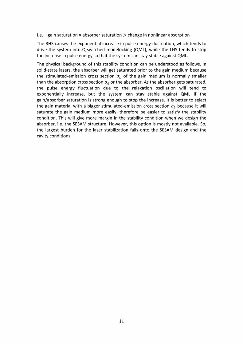
Group delay dispersion (GDD) is an important parameter for femtosecond pulses and soliton modelocking. If GDD is large, the ultrashort pulses (fs regime) can be significantly broadened. The GDD of SESAM is essentially determined by the bragg mirror structure of SESAM. In anti-resonant structures(FIG 3.7 (a)), the GDD curve is close to zero and flat over a wide range of wavelength. In resonant structures(FIG 3.7 (b)), on the other hand, the GDD typically has large values and its curve can violently fluctuate, the available range of operation wavelengths can be significantly

17

limited, which thus limits the shortest possible pulse length. Similar to the chirped mirrors [11], the structure of SESAM can be designed to have a negative GDD so that the pulse broadening in the other optical components, e.g. gain material, can be even compensated in the SESAM (Fig. 3.7 (c)).

Figure 3.7 Examples of Group delay dispersion (GDD) curves for (a) anti-resonant, (b) resonant, and (c) chirped structures.

3.3 Quantum Well (QW) SESAM vs. Quantum Dots (QD) SESAM

In the past, most of the SESAMs had quantum well (QW) absorbers. Recently, however, the interests in quantum dot (QD) have been growing since it can offer additional degrees of freedom in designing the SESAM parameters. In this section, I will compare them as the absorbers in SESAM devices, and point out the advantages of exploiting quantum dots rather than quantum well structures.

In quantum well absorbers, 𝐹𝑠𝑎𝑡 and ∆𝑅 are linked together to a large degree through the energy required to saturate the absorber, which is proportional to the density of states of the absorber because those states have to be filled up with charge carriers as photons are absorbed. Due to an intrinsic property of 2-dimensional case (Fig. 3.8), however, it is difficult to control the density of states in quantum wells (QW). Therefore 𝐹𝑠𝑎𝑡 and ∆𝑅 are significantly linked. Even if we manage to reduce 𝐹𝑠𝑎𝑡 , modulation depth ∆𝑅 will increase as much. In such cases, there is no benefit in terms of stability, because the product 𝐹𝑠𝑎𝑡 ∙ ∆𝑅 should decrease to give more margin in the stability condition Eq.(2.31).

Using quantum dots (QD), however, the density of states is simply proportional to the dot density. This novel property enables us to adjust the modulation depth ∆𝑅 independently with controlling the dot density (i.e. monolayer coverage) while the influence on saturation fluence 𝐹𝑠𝑎𝑡 remains negligible because the dot density doesn’t affect the absorption cross section 𝜎𝐴 of the QD. This has been demonstrated [12]. In addition, if we manage to control the size of QD, we can adjust the absorption cross section 𝜎𝐴 of the QD, thus, the saturation fluence 𝐹𝑠𝑎𝑡 . Indeed, it has been reported that the saturation fluence 𝐹𝑠𝑎𝑡 can be independently reduced by post-growth annealing, i.e. post-growth annealing changes the dot size.

0.98 1 1.02 1.04 1.06 1.08-500

-250

0

250

500

Wavelength [m]

GD

D

(fs

2)

1 1.01 1.02 1.03 1.04 1.05 1.06

-10000

-5000

0

5000

10000

Wavelength [m]

GD

D

(fs

2)

0.99 1 1.01 1.02 1.03 1.04 1.05 1.06-500

-400

-300

-200

-100

0

Wavelenth [m]

GD

D

(fs

2)

(a) (b)

(c)

18

𝑐𝑚−3𝑒𝑉−1

In addition to the success of quantum dot SESAMs, carbon nanotube (CNT) saturable absorber is also attracting the attention as an alternative solution [13]. The deeper investigation for their novel properties is expected to be done in the near future.

Figure 3.8 Density of states (DOS) per unit volume and energy for a 3D semiconductor (blue curve), a 10 nm quantum well with infinite barriers (red curve) and a 10 nm by 10nm quantum wire (e.g. CNT) with infinite barriers (green curve). The black line is DOS for the zero dimensional quantum dots. The picture is taken from [14].

19

C h a p t e r 4

SESAM STRUCTURE DESIGN

By now, the readers should be familiar with the backgrounds of this work and the terms which are often used in this thesis. In this chapter, I will show the SESAM design capability by simulating the field structures, group-delay dispersion (GDD), and linear reflectivity spectrum. The simulation is based on the transfer-matrix method, which is introduced in the first section of this chapter. The refractive indices of the structures are calculated by the Sellmeier equation so that the material dispersion is taken into account in the simulation.

4.1 Transfer Matrix Method

Field structures, reflectivity, GDD, and all the other features are simulated using the transfer-matrix formalism, which is based on the boundary conditions derived from Maxwell equations. If we take two traveling waves of the electric field (E±) as two components of a basis vector, one can easily arrive at interface matrices describing the boundary condition at each interface and propagation matrices describing propagation through layers of dielectric medium. For normal incidence, the relation between 𝐸1± and 𝐸𝑁± can be simply written as

𝐸1+

𝐸1− =

1

2

1 +𝑛2

𝑛11 −

𝑛2

𝑛1

1 −𝑛2

𝑛11 +

𝑛2

𝑛1

∙ 𝑒𝑖𝑘2𝑑2 00 𝑒−𝑖𝑘2𝑑2

∙1

2

1 +𝑛3

𝑛21 −

𝑛3

𝑛2

1 −𝑛3

𝑛21 +

𝑛3

𝑛2

∙ 𝑒𝑖𝑘3𝑑3 00 𝑒−𝑖𝑘3𝑑3

∙∙∙ 𝐸𝑁+

𝐸𝑁−

(4.1)

where 𝐸𝑁± are two traveling waves of the electric field in the opposite directions in Nth layer, 𝑛𝑁 and 𝑑𝑁 are refractive index and thickness of the Nth layer,

respectively, and 𝑘𝑁 =𝑤

𝑐𝑛𝑁 is wave vector in Nth layer. Absorption is taken into

account through the imaginary part of refractive index 𝑛 of the absorber layers.

4.2 Perturbation's point of view - resonant vs. anti-resonant

Considering Maxwell's equations as an eigenvalue problem, the small absorption can be treated as a perturbation to the solution. As a result, one can calculate the change of the eigenvalue and the mode profile, using the 1st-order perturbation theory that one could find in any quantum mechanics textbooks. Although this was not necessary for simulating SESAM behaviors since the transfer matrix method worked beautifully, it was worthwhile to double-check the result from the mere transfer matrix method, and moreover, the perturbation theory offered a deeper understanding on the difference between resonant and anti-resonant characteristics of SESAM structures. They will be explained and discussed in this section.

20

Let us start from the Maxwell's equations.

∇ × 𝐸 𝑟, 𝑡 + 𝜇0

𝜕𝐻(𝑟, 𝑡)

𝜕𝑡= 0

(4.2-a)

∇ × 𝐻 𝑟, 𝑡 − 휀0휀(𝑟)

𝜕𝐸(𝑟, 𝑡)

𝜕𝑡= 0

(4.2-b)

where the variables can be separated without losing generality as

𝐻(𝑟, 𝑡) = 𝐻 𝑟 exp(−𝑖𝜔𝑡) (4.3-a)

𝐸(𝑟, 𝑡) = 𝐸 𝑟 exp(−𝑖𝜔𝑡) (4.3-b)

From Eq.(4.2) and Eq.(4.3), one can easily obtain the time-independent expressions:

∇ × 𝐸 𝑟 − 𝑖𝜔𝜇0𝐻 𝑟 = 0 (4.4-a)

∇ × 𝐻 𝑟 + 𝑖𝜔휀0휀(𝑟)𝐸(𝑟) = 0 (4.4-b)

Eq.(4.4-a) and Eq.(4.4-b) can be merged into one equation:

∇ × ∇ × 𝐸 𝑟 =

𝜔

𝑐

2

휀 𝑟 𝐸(𝑟) (4.5-a)

or equivalently,

1

휀 𝑟 ∇ × ∇ × 𝐸 𝑟 =

𝜔

𝑐

2

𝐸(𝑟)

(4.5-b)

This now became an eigenvalue problem. We consider 1

휀 𝑟 ∇ × ∇ × as the operator

and 𝜔

𝑐

2

as the eigenvalue for corresponding eigenstates 𝐸(𝑟).

Now, adding a perturbation ∆휀 ≪ 휀,

1

휀 + ∆휀∇ × ∇ × 𝐸 𝑟 =

𝜔′

𝑐

2

𝐸(𝑟) (4.6)

LHS can be rewritten as:

1

휀 + ∆휀∇ × ∇ × 𝐸 𝑟 =

1

1 +∆휀휀

∙1

휀∇ × ∇ × 𝐸 𝑟

≈ 1 −

∆휀

휀 ∙

1

휀∇ × ∇ × 𝐸 𝑟 =

𝜔

𝑐

2

−∆휀

휀 𝜔

𝑐

2

𝐸(𝑟)

where I have used the Eq.(4.5-b). Now, Eq.(4.6) can be rewritten as:

𝜔2 − 𝜔2∆휀

휀 𝐸(𝑟) = 𝜔′2𝐸(𝑟)

(4.7)

Thus we obtained the perturbation operator −𝜔2 ∆휀

휀 .

Now, using the 1st-order perturbation theory, which can be found in most of quantum mechanics text books, we can calculate the change of eigenvalue 𝑑 𝜔2 :

21

𝑑 𝜔2 ≡ 𝜔′2 − 𝜔2 = 𝐸 −𝜔2 ∆휀

휀 휀𝐸

𝐸|휀𝐸 (4.8)

Because 𝜔′ ≡ 𝜔 + 𝑑𝜔 and 𝑑 𝜔2 ≡ 𝜔′2 − 𝜔2 ≈ 2𝜔𝑑𝜔, Eq.(4.8) can be rewritten as

𝑑𝜔 =

𝑑 𝜔2

2𝜔= −

𝜔

2

𝐸 ∆휀 𝐸

𝐸|휀𝐸 = −

𝜔

2 ∆휀 𝐸 2 𝑑3𝑟

휀 𝐸 2 𝑑3𝑟

(4.9)

or equivalently,

𝑑𝜆 =

𝜆

2 ∆휀 𝐸 2 𝑑3𝑟

휀 𝐸 2 𝑑3𝑟

(4.10)

When absorption is treated as a perturbation, ∆휀 must be a complex number since absorption is expressed through the imaginary part of refractive index. Therefore, the wavelength change 𝑑𝜆 due to absorption is also a complex number.

In the transfer matrix method, absorption is usually expressed through the imaginary part of refractive indices. As an alternative solution, one can exploit Eq.(4.10) in the transfer matrix method with real refractive indices only. In the latter case, the absorption is expressed through the wavelength which is a complex number. A comparison of the results for both cases can be used for a sanity check of the simulations.

As I checked the results for each cases with a small absorption coefficient, they produced exactly the same results (the same reflectivity, the same absorbance, etc.) as they should since both are basically derived from Maxwell's equations. But for large absorption coefficients ( ∆ε ≳ 휀 ), a discrepancy between them (i.e. the 1st-order perturbation theory and the transfer matrix method) is observed since the higher order terms of (∆휀/휀) cannot be just neglected in the formulation.

The perturbation method is unnecessary for our purpose of simulation, since the transfer-matrix method with complex refractive index is simpler and giving a correct result even for large absorption. The beauty and usefulness of the perturbation method, however, is not diminished because it gives an important insight to understand why anti-resonant structures are more stable, e.g. less sensitive to growth errors; Let us consider the growth errors as perturbation, ∆휀 will be the biggest near the interface between air and device when the growth errors happens. Anti-resonant structures, fortunately, have a node near the air-device interface, 𝑑𝜆 in the Eq.(4.10) would be much smaller compared to the resonant structure cases in which an anti-node is located at the air-device interface.

22

4.3 Results of Simulation - field structures, GDD, enhancement factors

In this section, I will demonstrate the SESAM design capability by showing the results of simulation for field structures, group-delay dispersion, and linear reflectivity spectrum. And I will also propose several novel QD-SESAM structures by using this simulation program I developed.

4.3.1 Demonstration: LOFERS (low-field-enhancement resonant-like SESAM device)

First of all, as an obvious sanity check, I have simulated the structures presented in the papers published from other groups, and proved my design capability by reproducing exactly the same results as they have published in those papers. I will show one example here selected from [15].

Low-field-enhancement resonant-like SESAM device (LOFERS) [16] has been chosen for my purpose of demonstration because the authors even have a patent for this simple structure, it is highly expected that this is a reliable object for a comparison. The structure specification is well given in [15]. They started with DBR of 30 pairs(GaAs/AlAs) with an additional top quarter-wave (80.8nm) GaAs spacer layer, followed by 10nm GaInAs absorber layer and 5nm GaAs protection cap. My simulation accurately reproduced their results of the standing wave pattern, the group delay dispersion (GDD), and the variation of enhancement factor. My results are presented in Fig 4.2. The readers are strongly encouraged to compare them with those in [15].

Figure 4.2 a) Refractive-index structure (black) near the surface and standing wave 𝑬𝒏 𝟐 pattern (blue) of the LOFERS for λ=1314nm have been reproduced for the demonstration.

Figure 4.2 b) The group delay dispersion curve has been reproduced for the demonstration.

0 0.5 1 1.5 20

1

2

3

4

Distance [m]

Norm

aliz

ed F

ield

Inte

nsity,

Refr

active index

1.26 1.28 1.30 1.32 1.34 1.36 1.38

-1000

-500

0

500

1000

Wavelength [m]

Gro

up d

ela

y d

ispers

ion (

fs2)

23

Figure 4.2 c) The variation of the enhancement factor has been reproduced for the demonstration.

Figure 4.2 d) Additionally, a linear reflectivity spectrum for small signals has been calculated.

Although a very minute variation in the results is possible, which must be caused by a slight change in the Sellmeier equations related to e.g. a given temperature, they are essentially the same results.

As I have proved that my simulation program is reliable, I became able to simulate any arbitrary SESAM structure on demand. In addition to the transfer matrix method, the strengths of my simulation program is that it is designed to be 'object-oriented', users don't need to care about transfer matrix algorithm for each cases. Users can simply tell any structures to the program just like putting Lego blocks together to create random structures. Each material is one function in Matlab with encapsulated information of its own properties inside. By virtue of this object oriented concept, implementations of any arbitrary structure became much faster and safer. All I had to do, since then, was to come up with new ideas for structure designs and tell the program what structure I want to see. In the next subsection, I will present some of the novel structures that I have designed using this simulation program.

1.26 1.28 1.3 1.32 1.34 1.36 1.380

1

2

3

4

Wavelength [m]

Enhancem

ent F

acto

r

24

4.3.2 Novel QD-SESAM structure: TAIGARS (tailored GDD anti-resonant-like SESAM device)

I present here a novel SESAM structures named “tailored GDD anti-resonant like SESAM device (TAIGARS)” which is a compromised solution to have all the advantages of both resonant and anti-resonant structures over reasonably wide operation bandwidth.

We start with a 30-pair DBR. Though the number of the pairs of this bottom DBR is not critical on the overall behavior of the device, it controls the amount of transmission of the structure. On the top of it, we add an approximately half-wave layer with the low-index material (AlAs) in which the InAs QD absorber layer is embedded at the center. The half-wave AlAs layer is followed by a shorter top DBR (Fig.4.3a).

Figure 4.3 a) Refractive-index structure (black) and calculated standing wave 𝑬𝒏 𝟐 pattern for λ=1030nm (red) of a TAIGARS. As shown in the top right corner of the picture, the QD layer is coated on both sides by 10nm GaAs layers for a practical reason in the fabrication.

Note that the standing wave in Fig.4.3a has a node near the surface of the TAIGARS as an anti-resonant like structure, which significantly reduces the surface scattering and the oxidation. This will also contribute to a better tolerance for the growth errors, which is of practical importance. Note also that the absorber layer is positioned at the maximum standing wave peak: 𝜉 ≅ 4.50. This exceeds the standing wave peak outside the device, which is extremely rare and interesting for an anti-resonant like structure. Compared to the classical SESAM device (𝜉 = 0.34) [15], this implies that the TAIGARS has the saturation fluence approximately 13 times lower, and the modulation depth 13 times higher if it has the same conditions of the absorber layer.

This structure designing could also heuristically be understood, step by step, starting from a resonant Gires-Tournois interferometer (GTI) as a springboard. First, the low-index material (AlAs) is chosen to be the top layer of the GTI so that it becomes an ‘anti-resonant’ structure. As a general property of GTI, there is no GDD exactly on anti-resonance. And then the number of the pairs in the top DBR is critically designed to keep very low GDD value over reasonably wide bandwidth around the anti-resonance (Fig.4.3b). It was also possible to make the structure slightly off the

0 1 2 3 4 5 6 70

1

2

3

4

5

R=98.9913% T=0.057391% A=0.9513% C=1030nm

Distance [m]

Nor

mal

ized

Fie

ld In

tens

ity,

Ref

ract

ive

Inde

x

2.1 2.2 2.3 2.4

25

anti-resonance by manipulating a layer thickness so that GDD becomes even slightly negative to compensate the dispersion from other optical elements inside the cavity such as a gain medium.

Figure 4.3 b) Calculated Group Delay Dispersion as a function of wavelength for a TAIGARS structure. The very low GDD around the operation wavelength λ=1030nm is one of the outstanding merits of this structure.

Figure 4.3 c) Calculated enhancement factor 𝝃 as a function of wavelength for a TAIGARS structure. It shows high field intensity over reasonably wide operation bandwidth.

Figure 4.3 d) Additionally, a linear reflectivity spectrum for small signals has been calculated.

Fig.4.3c shows the enhancement factor 𝜉 as a function of wavelength. Although it shows a mild resonant-like behavior, it maintains large enhancement factor (bigger than 3) over roughly more than 30 nm wide bandwidth. Compared to other various

1 1.02 1.04 1.06 1.08-1500

-1000

-500

0

500

1000

1500

Wavelength [m]

Gro

upe d

ela

y dis

pers

ion (

fs2)

1 1.01 1.02 1.03 1.04 1.05 1.06 1.070

1

2

3

4

5

Wavelength [m]

Enhancem

ent F

acto

r

26

kinds of structure, the most unique property of the TAIGARS must be its tailored Group Delay Dispersion (GDD) to exhibit very low GDD (from −300fs2 to +30fs2) over the reasonably wide bandwidth (20nm) despite of the very large enhancement factor.

4.3.3 Novel QD-SESAM structure: Anti-resonant QD SESAM variable to partly resonant by depositing SiO2

I present here another novel SESAM structure which is an Anti-resonant QD SESAM that can be easily switched to a partly resonant structure by depositing SiO2 on the top surface.

This anti-resonant QD-SESAM structure(Fig.4.4a) is similar to anti-resonant GTI, consisting of top antireflection GaAs/AlAs pairs, three QD layers embedded in GaAs spacer and positioned at the anti-nodes, followed by 28 pairs (GaAs/AlAs) of DBR designed for operation wavelength at 1030 nm.

Figure 4.4 a) Refractive-index structure (black) and calculated standing wave 𝑬𝒏 𝟐 pattern for λ=1030nm (red). The structure contains 3 layers of quantum dot absorber, which are positioned at the field anti-nodes.

Figure 4.4 b) Calculated group delay dispersion as a function of wavelength. As an anti-resonant structure, the GDD curve is relatively flat over a wide range around the operation wavelength at 1030nm.

0 1 2 3 40

1

2

3

4

Distance [m]

Norm

aliz

ed F

ield

Inte

nsity,

Refr

active index

0.99 1 1.01 1.02 1.03 1.04 1.05 1.06-1500

-1000

-500

0

500

1000

1500

Wavelength [m]

Gro

up d

ela

y d

ispers

ion (f

s2)

27

Figure 4.4 c) Calculated enhancement factor 𝝃 as a function of wavelength. It shows typical anti-resonant like behaviour.

Figure 4.4 d) A linear reflectivity spectrum for small signals has been calculated.

When it is necessary to adjust the saturation fluence for a particular laser design, this anti-resonant structure can be switched to a partly resonant structure simply by depositing SiO2 on the top surface. This procedure wouldn't require additional expensive MBE growth runs or etching steps, which are very likely to introduce additional defects on the surface.

After depositing approx. 0.213 µm SiO2 layer, the modified QD-SESAM will exhibits the following characteristics in Fig.4.5.

Figure 4.5 a) Refractive-index structure (black) and calculated standing wave 𝑬𝒏 𝟐 pattern for λ=1030nm (red). After depositing the SiO2 layer, the structure becomes partly resonant, the field intensity is now roughly twice as strong as the previous case in Fig 4.4a.

1 1.02 1.04 1.06 1.080

1

2

3

4

Wavelength [m]

Enhance

ment F

act

or

0 1 2 3 40

1

2

3

4

Distance [m]

Norm

aliz

ed F

ield

Inte

nsity

28

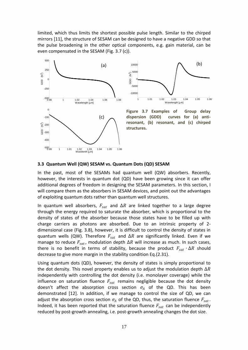
Figure 4.5 b) Calculated group delay dispersion as a function of wavelength. It shows a slightly negative value of GDD over more than 40nm around the operation wavelength λ=1030nm, which is very attractive and unusual for resonant structures. It seems even better than the anti-resonant case in Fig. 4.4b.

Figure 4.5 c) Calculated enhancement factor 𝝃 as a function of wavelength. It shows mild resonant like behaviour.

Figure 4.5 d) A linear reflectivity spectrum for small signals has been calculated.

0.99 1 1.01 1.02 1.03 1.04 1.05 1.06 1.07-1000

-500

0

500

1000

Wavelength [m]

Gro

up d

ela

y d

ispers

ion (

fs2)

1 1.02 1.04 1.06 1.080

1

2

3

4

Wavelength [m]

Enhancem

ent F

acto

r

29

C h a p t e r 5

SIMULATION OF SESAM SATURATION BEHAVIOUR

SOLVING ABSORBER RATE EQUATIONS

5.1 A simple model function for fitting measured data

The key parameters such as saturation fluence and modulation depth are usually obtained by fitting the measured nonlinear reflectivity to a simple model function [17] despite of several rather strong approximations used in the formulation of the model. In the derivation of this model function, they used a travelling wave model based on rate equations for a two-level system without relaxation, and neglected the effects of standing wave patterns in the device, which followed the formalism e.g. in [18]. This was a good approximation for a slow absorber such as Quantum Well, where the recovery time is much longer than the pulse bleaching the absorber [17, 19]. It must be questioned, however, for fast absorbers such as QD and Carbon nanotube as they are getting quite popular for building ultrafast lasers these days. Indeed, when the recovery time is not slow enough compared to the pulse duration, the definition of saturation fluence (i.e. 𝐹𝑠𝑎𝑡 = 𝑕𝑣/2𝜎eff ) becomes unclear since the saturation behavior is not exponential anymore. A brief summary of the model function based on the two-level system with slow absorbers is given below.

𝑅 𝐹𝑝 =𝐹𝑂𝑈𝑇

𝐹𝐼𝑁=

𝐼𝑂𝑈𝑇𝑑𝑡∞

−∞

𝐼𝐼𝑁∞

−∞𝑑𝑡

=ln(1 + 𝑅𝑙𝑖𝑛 (𝑒𝐹𝑝 𝐹𝑠𝑎𝑡 − 1))

𝐹𝑝 𝐹𝑠𝑎𝑡 (5.1)

where 𝑅𝑙𝑖𝑛 = exp(−∆𝑅) is the linear reflectivity for weak signals when there is no non-saturable loss. A real SESAM structure, however, always has some non-saturable losses which can be introduced by defects, residual transmission, scattering losses, and etc. These losses can effectively be taken into account in the model function by

a scaling factor 𝑅𝑛𝑠 . Substituting 𝑅 𝐹𝑝 /𝑅𝑛𝑠 and 𝑅𝑙𝑖𝑛 /𝑅𝑛𝑠 for 𝑅 𝐹𝑝 and 𝑅𝑙𝑖𝑛 ,

respectively, we have a corrected model function as follow:

𝑅 𝐹𝑝 = 𝑅𝑛𝑠

ln(1 +𝑅𝑙𝑖𝑛

𝑅𝑛𝑠(𝑒𝐹𝑝 𝐹𝑠𝑎𝑡 − 1))

𝐹𝑝 𝐹𝑠𝑎𝑡

(5.2)

Furthermore, nonlinear induced absorption (e.g. two photon absorption) can be accounted for simply by multiplying the model function with a factor exp(−𝐹𝑝/𝐹2),

where F2 is the fluence where the contribution of the induced absorption to the SESAM reflectivity drops to 1/e. A smaller F2 value corresponds to a stronger induced absorption (a stronger roll-off) [17].

30

5.2 Direct simulation

The simple model function above seems to work very well for slow absorbers like quantum wells [17]. The reliability of this method, however, should be questioned for fast absorbers like quantum dots, since the model function was started out on the assumption that the recovery time of absorbers was much slower than the pulse duration so that we could neglect any relaxation during the transit time of the pulse. The effects of standing wave and pulse shape were also neglected in the model function. To obtain more reliable expectations for the saturation behavior of fast QD SESAMs prior to actual fabrication, I directly calculated nonlinear reflectivity in Eq.(5.3) as follows:

𝑅 𝐹𝑝 =

𝐹𝑂𝑈𝑇

𝐹𝐼𝑁=

𝐼𝑂𝑈𝑇(𝑡)𝑑𝑡∞

−∞

𝐹𝑝

=

1

𝐹𝑝 𝐼𝑂𝑈𝑇(𝑡)

𝑡=∞

𝑡=−∞

=1

𝐹𝑝 𝑅 𝛼 𝑡 , 𝐼𝐼𝑁 𝑡 𝐼𝐼𝑁(𝑡)

𝑡=∞

𝑡=−∞

(5.3)

where the reflectivity 𝑅 𝛼 𝑡 , 𝐼𝐼𝑁 𝑡 is calculated at each time using my simulation

program, which is based on the transfer-matrix method described in the chapter 4. The strategy is as follows. First, an analytic solution for the saturation of absorption coefficient as a function of the transit time of the pulse is obtained by solving the rate equation Eq.(5.4). And then, the result is taken into account in transfer matrix method via the complex refractive index of the absorber while the program

calculates the reflectivity 𝑅 𝛼 𝑡 , 𝐼𝐼𝑁 𝑡 in the Eq.(5.3). This will take into account

the actual saturation behavior of fast absorbers as well as the standing wave effects and the incident pulse shapes 𝐼𝐼𝑁(𝑡). Let us start with finding an analytic solution for the saturation of the absorption coefficient.

As long as the absorption mechanism is based on the population difference ∆𝑁 of charge carriers, it can be well approximated as a two-level system. By analytically solving the differential equation Eq.(5.4) for two level systems [20], the saturation behavior of an absorber can be calculated as follows. (Note! a list of the parameters and their descriptions is given at the end of this section):

The rate equation: 𝑑∆𝑁

𝑑𝑡= −∆𝑁

1

𝜏+ 2𝑊(𝑡) +

𝑁𝑡

𝜏 (5.4)

Solution: ∆𝑁 𝑡 =𝑁𝑡

𝜏exp −

1

𝜏+ 2𝑊 𝑡′ 𝑑𝑡′

𝑡

𝑡0

× exp − 1

𝜏+ 2𝑊 𝑡′′ 𝑑𝑡′′

𝑡 ′

𝑡0

𝑑𝑡 ′𝑡

𝑡0

+ 𝜏

(5.5)

The differential equation Eq.(5.4) has a solution that is given in Eq.(5.5). And now one can calculate the absorption coefficient 𝛼(𝑣 − 𝑣0 , 𝑡) at a frequency 𝑣 and time 𝑡 as follows:

𝛼 𝑣 − 𝑣0 , 𝑡 = 𝜎∆𝑁 𝑡 (5.6)

where 𝛼0 = 𝜎0𝑁𝑡 is the unsaturated absorption coefficient at the resonant frequency 𝑣 = 𝑣0.

31

If we assume the homogenous broadening:

𝜎 = 𝑣

𝑣0

𝜎0

1 + 2 𝑣 − 𝑣0

∆𝑣0

2 (5.7)

Eq.(5.6) can be written together with Eq.(5.7):

𝛼 𝑣, 𝑡 = 𝜎∆𝑁 𝑡 = 𝜎0 𝑣

𝑣0

∆𝑁 𝑡

1 + 2 𝑣 − 𝑣0

∆𝑣0

2 (5.8)

= 𝜎0 𝑣

𝑣0

𝛼0

1 + 2 𝑣 − 𝑣0

∆𝑣0

2

∆𝑁 𝑡

𝑁𝑡

Substituting ∆𝑁 𝑡 /𝑁𝑡 in Eq.(5.5) into Eq.(5.8), one obtains an explicit form of the absorption coefficient as the pulse bleaching the absorber:

𝛼 𝑣 − 𝑣0 , 𝑡 =𝛼0

𝜏

𝑣

𝑣0

exp − 1𝜏 + 2𝑊 𝑡′ 𝑑𝑡′

𝑡

𝑡0

1 + 2 𝑣 − 𝑣0

∆𝑣0

2

× exp − 1

𝜏+ 2𝑊 𝑡′′ 𝑑𝑡′′

𝑡 ′

𝑡0

𝑑𝑡′𝑡

𝑡0

+ 𝜏 (5.9)

This time dependent absorption coefficient Eq. (5.9) will be taken into account via

the imaginary part of refractive index 𝑛𝑖𝑚𝑔 (𝑡) = 𝛼(𝑡)𝑐

2𝜔 in the transfer matrix

method. Then the simulation program which is based on the transfer matrix method

will produce the reflectivity 𝑅 𝛼 𝑡 , 𝐼𝐼𝑁 𝑡 as a function of the intensity. Here, the

transfer matrix method takes into account the standing wave effects. Next, the

program will integrate the reflectivity 𝑅 𝛼 𝑡 , 𝐼𝐼𝑁 𝑡 along the transit time of the

pulse to produce the nonlinear reflectivity curve 𝑅 𝐹𝑝 as a function of pulse

fluence. In this integration, the actual pulse shape 𝐼𝐼𝑁 𝑡 is taken into account. Therefore, the strong approximations in the simple model function Eq. (5.2) (i.e. a slow relaxation, no standing wave effects, a pulse shape ignored) are removed in this direct simulation.

Using this direct simulation tool, I will here present saturation behaviors for the TAIGARS (the SESAM structure which was described in section 4.3.2.) for the two cases, i.e. a slow absorber and a fast absorber. A comparison between the results from the simple model function Eq.(5.2) and the direct simulation Eq.(5.3) will be also presented.

32

A slow absorber: (the relaxation time 𝜏 = 1𝑝𝑠, the pulse width ∆𝜏𝑃 = 50𝑓𝑠)

Let us consider a 50𝑓𝑠 (FWHM) long pulse incident on the absorber with the relaxation time 𝜏 = 1𝑝𝑠. The pulse shape was assumed to be a square of the

hyperbolic-secant function (i.e. sech2 𝑡

1.76 ∆𝜏𝑃 ) as is the case for passively

modelocked lasers. Since the pulse length is 20 times shorter than the relaxation time of the absorber, the absorber is well considered to be a relatively slow absorber. As a strong two-photon absorption (TPA) occurs in GaAs, a reasonable value for the TPA coefficient 𝛽𝐺𝑎𝐴𝑠 = 40𝑐𝑚/𝐺𝑊 was taken from a literature [21], while the TPA in AlAs was neglected according to [22]. Reasonable values for Non-saturable loss, unsaturated absorption coefficient, and absorption cross-section were all assumed, which can be corrected any time with real material data. As a result, the calculated nonlinear reflectivity of TAIGARS is presented in Fig.5.1.

Figure 5.1 The calculated nonlinear reflectivity of TAIGARS(section 4.3.2) with a slow absorber. The black dotted line: the model function Eq.(5.2) described in section 5.1. The red solid line: the result from the direct simulation using Eq.(5.3). The blue dashed line: Eq.(5.3) with two photon absorption taken into account.

In Fig.5.1, 𝐹𝑆1 is the saturation fluence 𝐹𝑠𝑎𝑡 = 𝑕𝑣/2𝜎eff well defined for slow absorbers only. 𝐹𝑆2 is defined as the fluence when the value of the absorption coefficient drops to 1/e (37%) of the unsaturated value. 𝐹𝑆1 and 𝐹𝑆2 are essentially the same when the relaxation time of the absorber is much longer than the pulse duration. The black dotted line for Eq.(5.2.) and the red solid line for Eq.(5.3.) seem pretty well overlapped because the absorber in this case is relatively slow. 𝐹𝑆1 and 𝐹𝑆2 are not so different in this case as 𝐹𝑆1 ≅ 0.74𝜇𝐽/𝑐𝑚2 and 𝐹𝑆2 ≅ 0.83𝜇𝐽/𝑐𝑚2. Moreover, since the pulse is only 50𝑓𝑠 long, a strong TPA is observed in Fig.5.1.

0.01 0.1 1 10 100 3000.97

0.975

0.98

0.985

0.99

0.995

1

a0=2579.1/cm

0=1E-14cm2

eff=1.299E-13cm2

R=1.0002% Rns=0.55709% FS1

=0.74J/cm2 FS2

=0.83J/cm2

Fluence [J/cm2]

No

nlin

ea

r R

efle

ctivity

33

A fast absrober: (the relaxation time 𝜏 = 1𝑝𝑠, the pulse width ∆𝜏𝑃 = 5𝑝𝑠)

Now, let us consider a 5𝑝𝑠 (FWHM) long pulse incident on the absorber with the relaxation time 𝜏 = 1𝑝𝑠. Thus the absorber itself is the same as one in the previous case. But because now the pulse duration is much longer (5𝑝𝑠) than before (50𝑓𝑠), the absorber is considered to be relatively fast. Other conditions are given to be the same, i.e. the same sech2 pulse shape, the same absorption coefficient and cross-section, the same TPA coefficient, the same structure of SESAM, and etc. The simulation result for this case is presented in Fig.5.2.

Figure 5.2 The calculated nonlinear reflectivity of TAIGARS(section 4.3.2) with a fast absorber. The black dotted line: the model function Eq.(5.2) described in section 5.1. The red solid line: the result from the direct simulation using Eq.(5.3). The blue dashed line: Eq.(5.3) with two photon absorption taken into account.

As shown in Fig.5.2, The black dotted line for Eq.(5.2.) and the red solid line for Eq.(5.3.) do not overlap at all. 𝐹𝑆2 is roughly 10 times larger than 𝐹𝑆1 as 𝐹𝑆1 ≅0.74𝜇𝐽/𝑐𝑚2 and 𝐹𝑆2 ≅ 7.4𝜇𝐽/𝑐𝑚2. We can conclude that, for fast absorbers, the simple model function Eq.(5.2.) is significantly deviated from the direct simulation result which includes the actual relaxation process, the standing wave effects, and the actual pulse shape. Besides, since the pulse length is longer than before, the weaker TPA is observed in Fig.5.2 compared to Fig.5.1.

0.01 0.1 1 10 100 300

0.986

0.988

0.99

0.992

0.994

0.996

0.998

a0=2579.1/cm

0=1E-14cm2

eff=1.299E-13cm2

R=1.0002% Rns=0.55709% FS1

=0.74J/cm2 FS2

=7.41J/cm2

Fluence [J/cm2]

Nonlie

ar

Reflectivity

34

Wrapping up this section, it should be pointed out that, although the direct calculation using the simulation program can get rid of several strong assumptions and approximations, it, of course, still has some approximations. A band structure is approximated by a two-level system as mentioned above already, and intraband relaxation and temperature effects are neglected. Furthermore, it has been ignored that, as the absorber becomes saturated, the real part of the refractive index 𝑛𝑟 of the absorber must also change via the Kramers-Kronig relations. But this is a good approximation since the absorption is small enough (~1%) in most cases of interest, the change in 𝑛𝑟 due to a saturation is negligible.

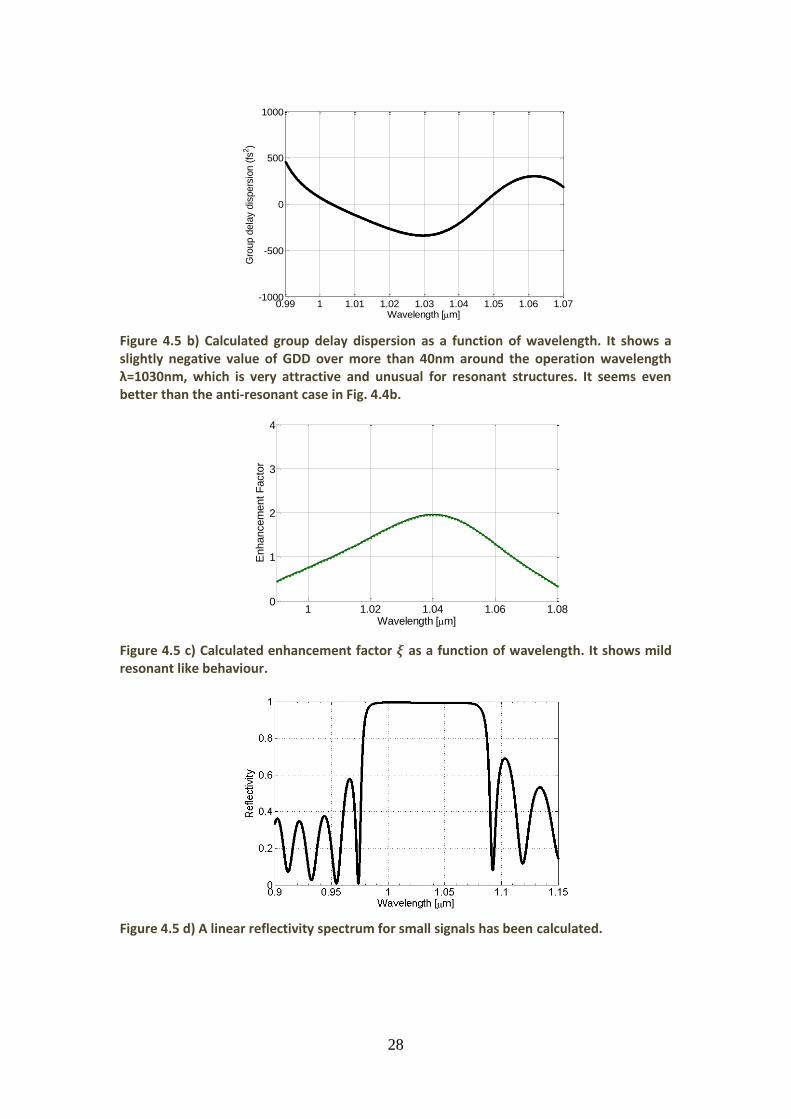
A brief summary of the parameters used in the equations is given below:

𝑣 : An operation frequency of the laser.

𝑣0: The transition frequency (i.e. at the absorption peak).

∆𝑣0: The linewidth (FWHM).

𝛼0: An absorption coefficient 𝛼 for small signals at 𝑣 = 𝑣0.

𝑊: Transition rate as a function of time, 𝑊 = 𝜎eff 𝐼(𝑡)/𝑕𝑣.

𝜎eff : Effective absorption cross section 𝜎eff = 𝑛𝑟𝝃𝜎0.

𝜎0: Absorption cross section of absorbers at the resonant frequency 𝑣 = 𝑣0.

𝜏 : Absorber relaxation time for spontaneous decay.

𝑛𝑟 : A real part of refractive index of the QD layer.

𝑁𝑡 : Total population of a two-level system 𝑁𝑡 = 𝑁1 + 𝑁2.

∆𝑁: Population difference ∆𝑁 = 𝑁1 − 𝑁2.

35

5.3 Self-Consistency

The reliability of my simulation program was checked by self-consistency of the loop in Fig. 5.3.

Figure 5.3 A loop for self-consistency. Modulation depth ∆R as an input should be reproduced as one of the outputs after the simulation.

As schematically described in Fig.5.3, I started with a desired value of modulation depth ∆𝑅, which is related to 𝛼0 according to Beer–Lambert law ∆𝑅 = 𝑛𝑟𝜉𝛼0𝑑 where 𝑑 is the thickness of a QD layer. Once the value of 𝛼0 is determined, one can calculate the time-dependent absorption coefficient 𝛼(t) according to Eq. (5.9) as saturation takes place. It is also required to determine absorption cross-section 𝜎0 with a reasonable value from the literatures e.g. [23] since it is included in the transition rate 𝑊 𝑡 = 𝑛𝑟𝝃𝜎0𝐼(𝑡)/𝑕𝑣 in Eq. (5.9). The absorption cross-section 𝜎0 is closely related to the saturation fluence 𝐹𝑠𝑎𝑡 ; for slow absorbers of two-level system,

we simply have 𝐹𝑠𝑎𝑡 =𝑕𝑣

2𝜎eff=

𝑕𝑣

2𝝃𝜎0.

As a next step, the imaginary part of the refractive index of the absorber is immediately determined at each moment of the transit time of the pulse according

to 𝑛𝑖𝑚𝑔 (𝑡) = 𝛼(𝑡)𝑐

2𝜔 where 𝜔 is angular frequency of the optical field. And then,

using 𝑛𝑖𝑚𝑔 (𝑡), one can finally calculate the nonlinear reflectivity in e.g. Fig.5.2 with

the simulation program which is based on the transfer-matrix formalism. After the simulation of the nonlinear reflectivity as a function of pulse fluence, the modulation depth ∆𝑅 is reproduced as one of the results. This reproduced ∆𝑅 should be self-consistent to its original value as an input data.

The self-consistency is, first, an obvious and important step to check the reliability of the simulation program. Second, this loop is also useful for extracting cross section values from the known designs and measurement data. Essentially there are four parameters: enhancement factor, absorber thickness, absorber refractive index, and cross section. Among those parameters, the cross section is least known one a priori.

o imgn

R

dnR r 0

2

cnimg

simulation using Eq.(5.3)

36

5.4 Quantum Dot Design?

When structure designs and measurement data of the saturation behavior are given, the required absorption coefficient and cross-section of the absorbers (e.g. quantum dots) can be calculated to achieve the measured modulation depth and saturation fluence. In other words, one can calculate the required QD parameters (e.g. 𝛼0, 𝜎0) to achieve the desired SESAM parameters (e.g. ∆𝑅, 𝐹𝑠𝑎𝑡 ). But this approach is not so practical since the relation between the growth parameters (e.g. growth-temperature, monolayer-coverage, annealing) in actual fabrications and the QD parameters has not been studied. Furthermore, those parameters may have difference correlations for different MBE reactors, different growth runs, and different wavelengths. For these reasons, it is difficult to give one-to-one transformation between the parameter spaces (Fig. 5.4) to pre-decide the SESAM parameters at the fabrication level.

Figure 5.4 The spaces of the parameters and unrevealed correlations between them. The relation between the SESAM parameters and the QD parameters can be confirmed by the simulation described in the previous sections.

Growth Parameters QD Parameters SESAM Parameters

Growth Temp. ML

Annealing

𝛼0 (Dot Density)

𝜎0 (QD size)

∆𝑅 𝐹𝑠𝑎𝑡

? !

?

37

C h a p t e r 6

LET THERE BE A LIGHT

BUILDING AND CHARACTERIZING A LIGHT SOURCE

In the previous chapters, the thesis has been focused on the theories and the computer simulations. From this chapter, I will focus on the experimental works I have done so far. I will explain the experimental setups and present the results. This chapter is assigned to introduce the supercontinuum fiber and its characteristics. Although this high-field science is very interesting subject on its own, it might seem a bit digression from the main context of this thesis which is the SESAM structure design and its characterization. This chapter, however, is practically of significant importance since a reliable light source is very much required for characterizing SESAM devices. 6.1 Light source using FemtoWHITE CARS PCF Fiber

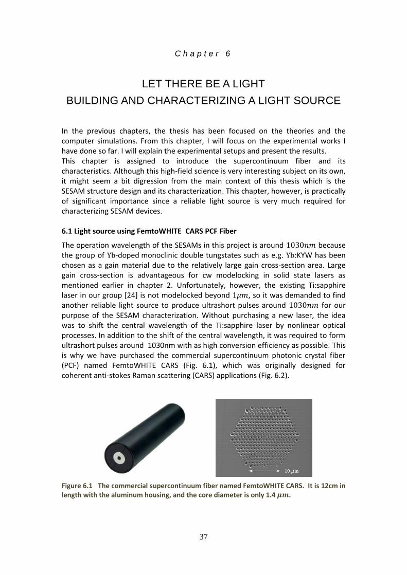
The operation wavelength of the SESAMs in this project is around 1030𝑛𝑚 because the group of Yb-doped monoclinic double tungstates such as e.g. Yb:KYW has been chosen as a gain material due to the relatively large gain cross-section area. Large gain cross-section is advantageous for cw modelocking in solid state lasers as mentioned earlier in chapter 2. Unfortunately, however, the existing Ti:sapphire laser in our group [24] is not modelocked beyond 1𝜇𝑚, so it was demanded to find another reliable light source to produce ultrashort pulses around 1030𝑛𝑚 for our purpose of the SESAM characterization. Without purchasing a new laser, the idea was to shift the central wavelength of the Ti:sapphire laser by nonlinear optical processes. In addition to the shift of the central wavelength, it was required to form ultrashort pulses around 1030nm with as high conversion efficiency as possible. This is why we have purchased the commercial supercontinuum photonic crystal fiber (PCF) named FemtoWHITE CARS (Fig. 6.1), which was originally designed for coherent anti-stokes Raman scattering (CARS) applications (Fig. 6.2).

Figure 6.1 The commercial supercontinuum fiber named FemtoWHITE CARS. It is 12cm in length with the aluminum housing, and the core diameter is only 1.4 𝝁𝒎.

38

In this PCF purchased, third-order parametric processes in a medium with a symmetric and rather steep GDD spectrum (see Fig. 6.4 (b)) result in two major peaks (see Fig. 6.4 (a)) located outside the two zero GDD points. This is what is required for CARS, and this is also what is required for the SESAM characterization.

Figure 6.2 Coherent Anti-stokes Raman Scattering (CARS) [25] is a third-order nonlinear optical process involving three laser beams: a pump beam at frequency ωp, a Stokes beam at frequency ωS and a probe beam at frequency ωpr. The interaction in the Raman medium is resonant at the anti-Stokes frequency (ωCARS = ωp-ωS+ωpr) when the frequency difference between the pump and the Stokes beams (ωp-ωS) coincides with the frequency (ωCARS -ωpr), which can be used for identifying the material.

In the setup (Fig. 6.3), the supercontinuum fiber was pumped by the Ti:sapphire laser of which pulses are measured to be 114 fs long by an autocorrelation measurement. The repetition rate of the pulses after the fiber is about 76MHz, which is the same as that of the Ti:sapphire laser. The pumping power was controlled with a λ/2 plate and the polarizing beam-splitter in the isolator. The input coupling efficiency around 35% was typically obtained using 20× microscope objective. One might be able to increase the efficiency by focusing the beam more tightly. The Damage threshold has not been confirmed, but the maximum pulse energy tried in [26] was approximately 1nJ for 40 fs, which corresponds to 2.5nJ for 100 fs for the same peak power. The maximum pulse energy I have achieved was around 1.2nJ when the average output power was 91mW. Considering the coupling efficiency (~35%), however, one can conclude that the entrance part of the PCF was exposed to the pulse energy higher than 3.4nJ. Thus it was preferred not to increase the pump power any further. After the supercontinuum fiber, another 10× microscope objective was used to collimate the output beam.

Figure 6.3 The implementation of the supercontinuum fiber (PCF) as a light source. The fiber is pumped by the existing Ti:sapphire laser. The typical coupling efficiency obtained was 35%.

𝜔CARS

𝜔stoke 𝜔p

𝜔pr

𝜔vib

B.S. B.S.

PCF

M.O.

Ti:sapphire Laser

F.R.

𝜆 2 M.O.

Mirror

isolator

39

6.2 Spectroscopy and data evaluation

In this section, I will first present the output spectrum after Supercontinuum fiber. Secondly, I will report the result of an autocorrelation measurement to estimate pulse length after the supercontinuum fiber followed by a long pass filter. Third, the observations on the state of polarization (SOP) will be presented. Fourth, I will show that the output spectrum is partly tunable by manipulating the pump power and/or its center wavelength. Lastly, an instability of the output spectrum and the output power will be reported. 6.2.1 Spectral depletion and special GVD curve

The black line in Fig. 6.4 (a) exhibits the output spectrum after the supercontinuum fiber without any filtering. The pump pulse centered at 852nm had pulse energy 600pJ with duration estimated to be 114 fs. As in the picture, the original pump field (red line) was completely depleted during its propagation along the fiber. The depletion region apparently corresponds to the anomalous GVD regime in Figure 6.4 (b). This spectral depletion over the wide range of the spectrum, i.e. roughly from 750nm to 950nm, results in two major peaks located outside the two zero GVD point. The small bump near 900nm is probably a leftover pump soliton red-shifted by Raman scattering.

Figure 6.4 (a) A general view of output spectrum (black line). In this particular measurement, the pump field (red line) was centered at 852nm with the pulse duration of 114fs. The spectrum beyond 𝟏𝝁𝒎 is used for the SESAM characterization after passing through a long pass filter.

600 700 800 900 1000 1100 12000

0.2

0.4

0.6

0.8

1

Wavelength (nm)

Norm

aliz

ed P

ow

er (a)

40

Figure 6.4 (b) The GVD curve of the fiber is taken from the reference [26], which corresponds to our photonic crystal fiber with two zero wavelength dispersion.

Figure 6.4 (c) The spectrum after the long pass filter at 𝟏𝝁𝒎.

6.2.2 Autocorrelation measurement for estimating the pulse length after PCF

The visible part of the spectrum in Fig. 6.4 (a) was filtered out by a long pass filter (LPF) at 1𝜇𝑚. The NIR part left after LPF was sent to an autocorrelator to measure the pulse length.

Figure 6.5 Autocorrelation trace of FWM idler at 1.03 µm showing pulse-length of 74 fs.

When an etalon (double pass) was inserted, the time shift was measured to be 1536 𝜇𝑠 on the oscilloscope while the real time shift due to the etalon for the double pass was given as 600fs.

If we conveniently assume that the shape of the pulse is a square of hyperbolic secant, we can calculate the pulse length as

600 fs ×296

1536×

1

1.543= 74.9352 fs ≈ 74.9 fs

950 1000 1050 1100 1150 12000

0.2

0.4

0.6

0.8

1

Wavelength (nm)

No

rma

lize

d P

ow

er

0 0.5 1 1.5 2 2.5 3 3.5 4-15

-10

-5

0

5

10

15

20

25

Time (ms)

mV

(b) (c)

41

6.2.3 Tunable Spectrum

The NIR part of the spectrum in Fig. 6.4 (a) will be used for the SESAM characterization after passing through a long pass filter (LPF). It will be advantageous if one can tune the spectrum to match to the various SESAM operation wavelengths.

Tunability by changing the central wavelength (𝜆pump ) of the pump field

The output spectrum was partly tunable by changing the central wavelength (𝜆pump )

of the pump field as shown in Figure 6.6. As the 𝜆pump increases, one can see the

tendency that the major peak splits into two parts, one moving left and another moving right in wavelength with respect to the 𝜆pump . Furthermore, the right peak

seems to become weaker as the 𝜆pump increases.

Figure 6.6 The Ti:sapphire laser (Tsunami) was tuned from 801.5nm to 852.5nm while the power coupled into the fiber was maintained around 50mW. The pulse length hasn't been measured for each cases assuming that they didn't change significantly from the previous measured value 114 fs.

42

Tunability by changing the pump power

It was also possible to tune the output spectrum by changing the power coupled into the fiber, or equivalently the peak power in the fiber. The pump power was controlled simply by using a half-wave plate and a polarizing beam splitter (PBS), while the coupling efficiency was maintained so that the peak power in the fiber is proportional to the incident pump power. It has been observed as shown in Fig. 6.7 that the frequency shift increases with the increasing pump power. At the same time, the shape of the spectrum also changes appreciably.

Figure 6.7 The pump power was changed from 33mW to 91mW while the coupling efficiency is maintained. The pump wavelength was centered and fixed at 806.8nm. The major peak moves further into the IR region (from 1050nm to 1116nm) with increasing pump power.

The spectral data shown in Fig. 6.7 is slightly noisy because the output beam was intentionally not focused for the fiber coupling to the spectrum analyzer so that a constant coupling efficiency can be obtained over the wide range of spectrum. 6.2.4 Different state of polarization (SOP) for different part of the spectrum

Although an ideal fiber with perfect cylindrical symmetry must have the identical refractive indices 𝑛𝑥 and 𝑛𝑦 for two orthogonally polarized modes, all fibers in

practice have some modal birefringence (𝑛𝑥 ≠ 𝑛𝑦 ) because of unintentional

variation of the core shape and anisotropic tensions along the fiber [27]. Thus, the state of polarization (SOP) of light propagating in fibers is generally elliptical. Furthermore, when ultrashort pulses propagate in a fiber, the SOP can be different for different parts of the pulse and spectrum due to the nonlinear birefringence in the fiber.

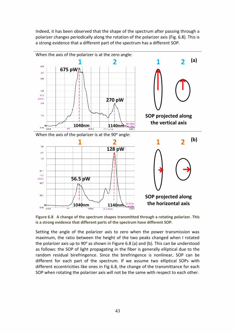
43

Indeed, it has been observed that the shape of the spectrum after passing through a polarizer changes periodically along the rotation of the polarizer axis (Fig. 6.8). This is a strong evidence that a different part of the spectrum has a different SOP.

When the axis of the polarizer is at the zero angle:

When the axis of the polarizer is at the 90ᵒ angle:

Figure 6.8 A change of the spectrum shapes transmitted through a rotating polarizer. This is a strong evidence that different parts of the spectrum have different SOP.

Setting the angle of the polarizer axis to zero when the power transmission was maximum, the ratio between the height of the two peaks changed when I rotated the polarizer axis up to 90ᵒ as shown in Figure 6.8 (a) and (b). This can be understood as follows: the SOP of light propagating in the fiber is generally elliptical due to the random residual birefringence. Since the birefringence is nonlinear, SOP can be different for each part of the spectrum. If we assume two elliptical SOPs with different eccentricities like ones in Fig 6.8, the change of the transmittance for each SOP when rotating the polarizer axis will not be the same with respect to each other.

56.5 pW

128 pW

1040nm 1140nm

675 pW

270 pW

1040nm 1140nm

(a)

SOP projected along the vertical axis

(b)

SOP projected along the horizontal axis

1 2 1 2

1 2 1 2

44

6.2.5 Instability of the output power and the output spectrum

It was often found that the output power and output spectrum change appreciably during the long term measurements. The reason for both can be attributed to the change of the fiber coupling efficiency, but the reason for the coupling efficiency drop hasn't been clearly confirmed yet. A slight beam shift from the Ti:sapphire laser is the most probable senario because a sub-micrometer beam shift can significantly affect the coupling efficiency due to the very small core diameter (1.4𝜇𝑚).

Measured at 3:11pm

Maximum power: 2.46mW

Measured at 6:14pm

Maximum power: 1.40mW

Figure 6.9 The supercontinuum output spectrum after passing through the LPF at 1000nm and the SPF at 1050nm (a) measured at 3:11pm, (b) measured at 6:14pm

Figure 6.9 shows one record of this instability. The output power and the spectrum after passing through the long pass filter (LPF) at 1000nm and the short pass filter (SPF) at 1050nm was measured twice: at 3:11pm and 3 hours later at 6:14pm without touching any part of the system. After the 3 hours, the power drop was as big as 43%, and the spectrum has shifted approximately 5nm towards the shorter wavelength.

To quantify the instability of the fiber coupling between the Ti:sapphire laser and the supercontinuum fiber, the coupling efficiency drop was measured as a function of time (Fig. 6.10). This measurement was conducted 10 hours after the Ti:sapphire laser started the operation. Thus one may conclude that the system was stabilized.

(a)

(b)

Wavelength

Wavelength

45

Figure 6.10 The center wavelength of the pump laser was centered at 806.8nm during the measurement. The pump power 249mW was also fixed during the measurement. When the measurement was started, the output power was 91mW. After 127 minutes, the output power dropped to 80mW. The fluctuation of the coupling efficiency was calculated as 𝟏𝟎𝟎% × 𝐬𝐭𝐚𝐧𝐝𝐚𝐫𝐝 𝐝𝐞𝐯𝐢𝐚𝐭𝐢𝐨𝐧 𝐚𝐯𝐞𝐫𝐚𝐠𝐞 𝐜𝐨𝐮𝐩𝐥𝐢𝐧𝐠 𝐞𝐟𝐟𝐢𝐜𝐢𝐞𝐧𝐜𝐲 = 0.75 %.

As shown in Fig. 6.10, the coupling efficiency has dropped as much as 4.42%. This absolute difference corresponds to 12.1% relative to the initial value.

The Fig 6.9 and the Fig 6.10 are, in fact, only the examples of the instability in using the supercontinuum fiber as a light source. The results can vary, depending on e.g. the pump power, the initial coupling efficiency, or the condition of the pump laser.

One could try an active beam stabilization system to maintain a constant coupling efficiency to the supercontinuum fiber. In my setup, however, the setup had a limited space, implementation of the active beam stabilization system was not feasible.

In chapter 7, this fluctuation in the output power and the spectrum will explain the measurement errors which is bigger than the error expected from the vertical memory in the oscilloscope.

0 20 40 60 80 100 120 14032

33

34

35

36

37

100% standard deviation / coupling efficiency =0.75%

time (min)

Couplin

g e

ffic

iency (

%)

46

C h a p t e r 7

SESAM CHARACTERIZATION

In the previous chapter, I presented the implementation of the supercontinuum fiber as a light source and its characterization. Using the supercontinuum fiber as a light source, I built an interferometric setup to measure the nonlinear reflectivity of SESAMs. This SESAM characterization setup will be explained in this chapter, including how to align it and how to calibrate. The reflectivity of a commercial SESAM device [28] has been measured as a function of incident fluence, and the result will be presented in this chapter. I will also evaluate the data by fitting them to the model equation Eq.(5.2) to determine the SESAM parameters. Lastly, some limitations due to the supercontinuum fiber used as the light source will be discussed.

7.1 SESAM characterization setup

I have implemented the SESAM characterization setup based on the one in [9]. As shown in Fig. 7.1, the beam is incident on an attenuator followed by a long pass filter (LPF). At the LPF, the visible part (<1𝜇𝑚) of the spectrum (Fig. 6.4 (a)) is removed leaving the NIR part (>1𝜇𝑚). The NIR part of the beam is split into two arms at the beam splitter (BS). SESAM and a High Reflection (HR) mirror are positioned at each arms, respectively, with normal incidence of the signals. A low-cost metallic silver mirror can be employed as the HR mirror. The reflectivity of the SESAM is obtained by measuring the responses from both arms and calculating the ratio between them. Although the setup looks similar to the Michelson interferometer, this reflectivity measurement is not exploiting any concept of interference because the signals from the two arms are periodically separated in time by a chopper. This setup is simpler compared to the one [17] where the signals are separated in space. In the latter case, two detectors are needed to measure both signals (i.e. incident and reflected) simultaneously, and a calibration of them is required.

Figure 7.1 A schematic description for the SESAM characterization setup. The optical elements are slightly tilted to keep the back reflection from the detector.

Figure 7.2 The SESAM characterization setup. The reflectivity of the SESAM is obtained by measuring the responses from both arms and the ratio between them.

HR Mirror

Detector/CCD

Attenuator

LPF SESAM

Lens

BS

Chopper

47

The supercontinuum fiber is used as a light source, which is described in the chapter 6. The maximum output power around 91mW right after the fiber has been achieved. It is first limited by the damage threshold of the fiber as discussed in section 6.1. After collimation and passing through the long pass filter followed by a few optical elements such as the attenuator, the beam splitter, and the lens, the actual maximum power incident on the SESAM is around 8mW at the best. Since the maximum incident power is limited, it is necessary to focus the beam tight on the SESAM surface. The required spot size at the beam waist to achieve a certain fluence can be calculated as follows:

Pulse Fluence =

Incident Average Power

Repetition Rate×

1

Beam Spot Size

(7.1)

To achieve the fluence of 100𝜇𝐽/𝑐𝑚2 with the maximum incident power of 8mW, the required beam radius is calculated as :

radius = 1

π×

8mW

76MHz×

1

100𝜇𝐽/𝑐𝑚2= 5.79𝜇𝑚

(7.2)

Similarly, to achieve 1000𝜇𝐽/𝑐𝑚2, the beam has to be focused down to :

radius = 1

π×

8mW

76MHz×

1

1000𝜇𝐽/𝑐𝑚2= 1.83𝜇𝑚

(7.3)

As shown in Fig 7.1, the SESAM arm is designed to be much longer than the HR arm to increase the divergence of the sample beam in the SESAM arm. This typically results in a smaller beam waist area after the lens. This is how I focused the beam tightly on the SESAM. The beam radius 3 ± 0.7𝜇𝑚 has been achieved using an aspherical lens with 7.5mm focal length. As the beam is focused tighter, however, the precise estimation of the beam spot size becomes even harder than focusing itself. This will be discussed in the section 7.4.

For an attenuator, a graded neutral density filter without beam translation is the best. The attenuators based on polarization filtering optics are not suitable in our case because the supercontinuum fiber is not polarization-maintaining, i.e. the polarization state after the fiber usually varies randomly during the measurement.

After the attenuator, the beam passes through a long pass filter (LPF) where the cut-off wavelength is 1𝜇𝑚. The NIR part of the beam continues propagating and then splits into two arms at a beam splitter. A chopper rotating with a frequency around 99Hz is positioned right behind the beam splitter. Position and tilted angle of the chopper is adjusted so that one cycle of the rotation produces four different states of measurements as shown in Fig. 7.3 (a). First, the chopper blocks both beams. Only the background noise level will be measured in this case. Second, the chopper blocks the reference beam to the HR mirror. The response from the SESAM and noise will be measured. Third, the chopper doesn't block any beam. Both beams with the background noise will be measured. This level is useful for checking the linearity of the detector. Lastly, the chopper blocks the beam incident on the SESAM. The reference response from the HR mirror and the background noise will be measured.

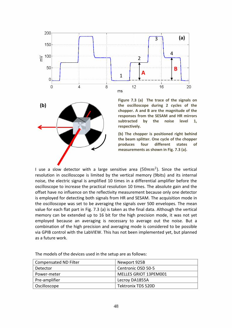
48

(b)

Figure 7.3 (a) The trace of the signals on the oscilloscope during 2 cycles of the chopper. A and B are the magnitude of the responses from the SESAM and HR mirrors subtracted by the noise level 1, respectively.

(b) The chopper is positioned right behind the beam splitter. One cycle of the chopper produces four different states of measurements as shown in Fig. 7.3 (a).

I use a slow detector with a large sensitive area (50𝑚𝑚2). Since the vertical resolution in oscilloscope is limited by the vertical memory (9bits) and its internal noise, the electric signal is amplified 10 times in a differential amplifier before the oscilloscope to increase the practical resolution 10 times. The absolute gain and the offset have no influence on the reflectivity measurement because only one detector is employed for detecting both signals from HR and SESAM. The acquisition mode in the oscilloscope was set to be averaging the signals over 500 envelopes. The mean value for each flat part in Fig. 7.3 (a) is taken as the final data. Although the vertical memory can be extended up to 16 bit for the high precision mode, it was not yet employed because an averaging is necessary to average out the noise. But a combination of the high precision and averaging mode is considered to be possible via GPIB control with the LabVIEW. This has not been implemented yet, but planned as a future work.

The models of the devices used in the setup are as follows:

Compensated ND Filter Newport 925B

Detector Centronic OSD 50-5

Power-meter MELLES GRIOT 13PEM001

Pre-amplifier Lecroy DA1855A

Oscilloscope Tektronix TDS 520D

(a)

1

2

3

4

A B

49

7.2 Alignment and calibration

In this section, the alignment of the setup after the supercontinuum fiber will be explained. I will discuss how to calibrate the system when either a polarizing or a non-polarizing beam splitter is employed.

7.2.1 Alignment

The microscope objective for the collimation is positioned in such a way that the focus of the reference beam lies on the HR mirror. In this case the incident and reflected beams are well overlapped in position and divergence, which can be checked using a thin glass piece. During the alignment, a CCD is positioned instead of a detector. The beam profile can be checked with a CCD to minimize the aberration by adjusting the microscope objective laterally.

Now working on the SESAM arm, the sample beam is aligned parallel to the optics table, and a translational stage is inserted with a lens on it. After fixing the translational stage, one can find the lens position so that the incident beam is hitting in the middle of the lens with the normal incidence. And then the lens is removed by moving the translational stage. Now, the SESAM is positioned right after the translational stage. Using an aperture and the back-reflection from the SESAM, one can adjust the SESAM perpendicular to the incident beam. The lens is inserted back again by moving back the translational stage, adjusting it with respect to the aperture. Now, the lens is moved along the beam propagation direction to locate the beam waist at the SESAM surface. When the both beams are focused onto the SESAM and the HR mirror respectively, the q parameters of the two beams in the detection arm should be the same, so are the images on CCD.

7.2.2. Calibration

Using another HR mirror at the SESAM position, one can calibrate the system. In an ideal case, the reflectivity measured using two identical HR mirrors should result in 1, independent of the incident fluence. In practice, however, each arm has different amount of losses due to e.g. the lens in the one arm. The system should be calibrated to take them into account as follows:

C ≡

BHR

AHR

(7.4)

where A and B are the magnitudes of the signal after subtracting the noise level as shown in Fig 7.3 (a). The calibrated reflectivity of SESAM can be calculated as follows:

RSESAM = RHR × C ×

ASESAM

BHR

(7.5)

where RHR is the reflectivity of the silver mirror in this case, which is about 99% around the operation wavelength 1040nm.

50

SESAM

HR Detector

When a piece of glass is used for the beam splitter (Fig. 7.4), there is an additional calibration factor which depends on the polarization of the incident light.

Figure 7.4 A glass (CaF2) piece used as a beam splitter. The reflection and refraction via the Stokes treatment introduce the additional calibration factor which depends on the polarization of the incident light.

Because the Fresnel coefficients are polarization-dependent, this polarization dependency can be calculated using Stockes Relations [29] as follows.

Calibration factor: Cpolarization =BHR

AHR∝

𝑟 𝑡 𝑡′ 2

𝑡 𝑡′ 𝑡 𝑟′𝑡′ 2=

1

𝑡 𝑡′ 2=

1

1 − 𝑟2 2 (7.6)

where the Fresnel coefficients 𝑟 and 𝑡 are the amplitude reflection and transmission coefficients, respectively, for a light incident from air to the glass. 𝑟′ and 𝑡′ are the same coefficients as 𝑟 and 𝑡, respectively, but for a light incident from the glass inside.

Similarly, whenever the beam splitter is polarization sensitive, there is always some additional calibration factor similar to Eq.(7.6). This is the reason that we have to use non-polarizing beam splitter when the polarization state is not stable.

The incident fluence must be proportional to BHR , i.e. the voltage of the response from the HR arm subtracted by the noise level.

Incdient fluence ∝ BHR (7.7)

One can calculate the coefficient of the proportionality in Eq.(7.7) by a linear fitting between BHR and the incident power measured by a power meter.

Figure 7.5 The incident fluence was corrected by a linear fitting between 𝐁𝐇𝐑 and the incident power measured by a power meter.

0 1 2 3 4 5 60

50

100

150

200

Incident Power measured by a Power-meter (mW)

BH

R (

mV

)

SESAM

HR Detector

51

7.3 Results and Discussion

In the measurements in this thesis, the commercial quantum well (QW) SESAM device from BATOP [29] has been employed to demonstrate the SESAM characterization setup I have built. It is expected to be easier to see the saturation behavior with the QW SESAM, because it typically has a bigger modulation depth than that of a quantum dot (QD) SESAM.

The linear reflectivity given in the product data sheet is presented in Fig. 7.6.

Figure 7.6 Low intensity linear reflectivity curve of the commercial Batop SESAM. The graph is given in the data sheet.

Using this SESAM, the setup described in the previous sections has been tested. In Fig. 7.7, I first present the result after the measurement using the piece of glass (CaF2) as a beam splitter (Fig. 7.4). The glass piece was originally preferred because it allowed a higher maximum power incident on the SESAM due to the high transmission/reflection ratio.

Figure 7.7 Nonlinear reflectivity measurement conducted using a glass piece as a beam splitter. A large modulation due to the unstable polarization state is observed.

10 1000.9

0.905

0.91

0.915

0.92

0.925

0.93

0.935

0.94

0.945

Fluence (J/cm2)

Reflectivity

52

In this case, the attenuator can be implemented using two polarizers which have a flat spectral response. The result is presented in Fig. 7.7 where the large modulation is obviously not a typical saturation behavior of the SESAM. After the discussion and the observation presented in chapter 6, I conclude that this result must originate from the supercontinuum fiber which is not polarization-maintaining. Since the fiber is not polarization-maintaining, the state of polarization (SOP) can easily change by slight changes in the coupling efficiency or changes even in the temperature inside the fiber. This nonlinear polarization rotation will change the calibration factor in Eq.(7.6), which results in the big modulation in Fig. 7.7. Thus, it was required to use non-polarizing beam splitter for a polarization-insensitive measurement.

Using the same QW SESAM, I conducted the same measurement but with a non-polarizing beam splitter. In this case, a compensated ND filter [30] was employed as an attenuator. It is important that the attenuator does not change the beam profile and beam propagation direction, which may cause serious errors in the result. The result is presented in Fig. 7.8. The maximum achievable pulse fluence was around 230μJ/cm2 when the beam radius was focused down to 3𝜇𝑚 onto the SESAM.

Figure 7.8 Nonlinear reflectivity measurement conducted using a non-polarizing beam

splitter. The maximum pulse fluence was around 𝟐𝟑𝟎𝛍𝐉/𝐜𝐦𝟐 with the beam radius around 𝟑𝝁𝒎 on the SESAM surface.

Fig. 7.8 doesn't exhibit error bars because there are several potential error sources which are difficult to be estimated. Thus, I will exhibit the standard deviation of the data with respect to the fitting function as a measure of the precision in this measurement. Since the incident pulse duration estimated to be approximately 74 fs is much shorter than the relaxation time of the quantum well (~ picoseconds), the data shown in Fig. 7.8 can be fitted to the simple model function in Eq.(5.2) with an additional factor exp(−𝐹𝑝/𝐹2) due to the induced absorption such as TPA:

𝑅 𝐹𝑝 = 𝑅𝑛𝑠

ln(1 +𝑅𝑙𝑖𝑛

𝑅𝑛𝑠(𝑒𝐹𝑝 𝐹𝑠𝑎𝑡 − 1))

𝐹𝑝 𝐹𝑠𝑎𝑡 exp(−𝐹𝑝/𝐹2)

(7.8)

10 100 10000.9

0.91

0.92

0.93

0.94

0.95

Fluence [J/cm2]

Reflectivity

53

The least square method was used in writing the fitting code in Matlab.

Figure 7.9 The data in Figure 7.8 is fitted to the simple model function in Eq.(5.2). The maximum achievable fluence is not high enough to determine the exact saturation behavior. Only two possible examples (solid and dashed line pairs) are presented in this figure. The red line is for two photon absorption (TPA) taken into account, while the blue line is without TPA.

As illustrated in Fig. 7.9, unfortunately, the maximum achievable fluence is not high enough to determine the exact saturation behavior. The results depends on the seed parameters to start with, or the allowed intervals of the parameters. I present only two examples in Fig 7.9 which are the solid line pair and the dashed line pair.

Solid line pair in Fig. 7.9. Dashed line pair in Fig. 7.9.

∆𝑅 2.88% 2.32%

∆𝑅𝑛𝑠 5.50% 6.10%

𝐹𝑆 90.8μJ/cm2 63.7μJ/cm2

error 0.065% 0.068%

Table 7.1 The SESAM parameters extracted by the fittings in Fig. 7.9.

According to [9] and [17], the pulse fluence of more than 10 times FS is required for a reliable parameter extraction. Furthermore, fluence of up to 50 times FS can be required when there is a strong TPA. If the FS of our QW SESAM is around e.g. 60μJ/cm2, then fluence higher than 600μJ/cm2 is required to obtain a precise parameter extraction. As shown in Fig. 7.8, the maximum achievable fluence in our setup was only around 230μJ/cm2 with the beam radius as small as 3μm at the beam waist. Thus, I can only conclude that the ranges in Table 7.2 are obtained when I limit the modulation depth ∆𝑅 smaller than 3%, which is a reasonable limit according the linear reflectivity curve in Fig. 7.6, and the error less than 0.1%.

10 100 1000 100000.9

0.91

0.92

0.93

0.94

0.95

Fluence [J/cm2]

Reflectivity

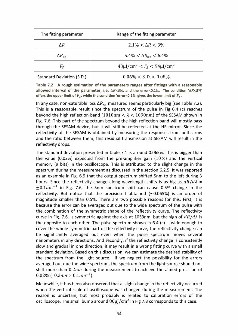
54

The fitting parameter Range of the fitting parameter

∆𝑅 2.1% < ∆𝑅 < 3%

∆𝑅𝑛𝑠 5.4% < ∆𝑅𝑛𝑠 < 6.4%

𝐹𝑆 43μJ/cm2 < 𝐹𝑆 < 94μJ/cm2

Standard Deviation (S.D.) 0.06% < S. D. < 0.08%

Table 7.2 A rough estimation of the parameters ranges after fittings with a reasonable allowed interval of the parameter, i.e. ∆𝑹<3%, and the error<0.1%. The condition '∆𝑹<3%'

offers the upper limit of 𝑭𝑺, while the condition 'error<0.1%' gives the lower limit of 𝑭𝑺.

In any case, non-saturable loss ∆𝑅𝑛𝑠 measured seems particularly big (see Table 7.2). This is a reasonable result since the spectrum of the pulse in Fig 6.4 (c) reaches beyond the high reflection band (1010nm < 𝜆 < 1090𝑛𝑚) of the SESAM shown in Fig. 7.6. This part of the spectrum beyond the high reflection band will mostly pass through the SESAM device, but it will still be reflected at the HR mirror. Since the reflectivity of the SESAM is obtained by measuring the responses from both arms and the ratio between them, this residual transmission at SESAM will result in the reflectivity drops.

The standard deviation presented in table 7.1 is around 0.065%. This is bigger than the value (0.02%) expected from the pre-amplifier gain (10 ×) and the vertical memory (9 bits) in the oscilloscope. This is attributed to the slight change in the spectrum during the measurement as discussed in the section 6.2.5. It was reported as an example in Fig. 6.9 that the output spectrum shifted 5nm to the left during 3 hours. Since the reflectivity change along wavelength shifts is as big as 𝑑𝑅/𝑑𝜆 ≈±0.1𝑛𝑚−1 in Fig. 7.6, the 5nm spectrum shift can cause 0.5% change in the reflectivity. But notice that the precision I obtained (~0.065%) is an order of magnitude smaller than 0.5%. There are two possible reasons for this. First, it is because the error can be averaged out due to the wide spectrum of the pulse with the combination of the symmetric shape of the reflectivity curve. The reflectivity curve in Fig. 7.6. is symmetric against the axis at 1053nm, but the sign of 𝑑𝑅/𝑑𝜆 is the opposite to each other. The pulse spectrum shown in 6.4 (c) is wide enough to cover the whole symmetric part of the reflectivity curve, the reflectivity change can be significantly averaged out even when the pulse spectrum moves several nanometers in any directions. And secondly, if the reflectivity change is consistently slow and gradual in one direction, it may result in a wrong fitting curve with a small standard deviation. Based on this discussion, we can estimate the desired stability of the spectrum from the light source. If we neglect the possibility for the errors averaged out due the wide spectrum, the spectrum from the light source should not shift more than 0.2𝑛𝑚 during the measurement to achieve the aimed precision of 0.02% (=0.2𝑛𝑚 × 0.1𝑛𝑚−1).

Meanwhile, it has been also observed that a slight change in the reflectivity occurred when the vertical scale of oscilloscope was changed during the measurement. The reason is uncertain, but most probably is related to calibration errors of the oscilloscope. The small bump around 80μJ/cm2 in Fig 7.8 corresponds to this case.

55

7.4 Limitations

Although the limitations encountered in the measurement were mentioned in the previous sections, I will highlight those limitations again in this section as they are important issues for the continuation of this project. Most of the limitations are considered to be originating from the supercontinuum fiber used as the light source.

The output power from the supercontinuum fiber is essentially limited because the operation regime was preferred to stay far from the possible damage threshold of the photonic crystal fiber as discussed in section 6.1. Furthermore, roughly more than 70% of the output power corresponds to the visible part of the spectrum, this part is filtered away leaving only 30% of the output power for our measurements. This results in a limitation on the maximum achievable pulse fluence. Even when the beam radius was managed down to 3μm, the maximum fluence achieved was only around 230μJ/cm2 for the maximum incident power of 6.1mW. The required maximum fluence estimated in the previous section for a reliable parameter extraction was at least ~600μJ/cm2.

It should also be pointed out that the precise estimation of the beam spot size using the knife edge method becomes challenging when the beam was focused very hard down to the beam radius of 3μm. The standard deviation of the beam size measurement was as big as 0.7μm in the Rayleigh range when it was fitted to the generalized Gaussian beam in Eq.(7.9).

𝜔𝐺 𝑧 = 𝜔𝐺0 1 + 𝑀2𝜆

𝜋𝜔𝐺02 𝑧

2

(7.9)

Although the 0.7μm measurement error is reasonable in the knife edge method, which can be caused by the aberrations and the limited precision in the translational stage, it results in a huge percentage error (22%) at the beam waist because the beam spot size at the waist is very small in this case. Even though this error is completely independent of other measurement errors, 60% error in the estimation of the beam spot area will result in 60% error in the saturation fluence. Therefore, the precision of the beam size measurement has to be improved, or the beam spot size should be increased for a better precision.

Figure 7.10 The beam size measurement using the knife edge method. The 𝑴𝟐 factor obtained from the fitting was approximately 𝟐. 𝟏𝟏.

0 1 2 3 4 5 6 7 8 90

0.2

0.4

0.6

0.8

1

1.2

1.4x 10

-3

z [mm]

w [m

]

56

If we increase the beam spot size up to e.g. 5μm for a better precision, the beam

spot area will increase 25

9 times, then

25

9 times higher incident power is required to

maintain the same pulse fluence. In this case, to achieve the pulse fluence 600μJ/cm2 in the previous discussion, the maximum achievable incident power (6.1mW) will have to be increased up to 45mW at least. If the 50:50 beam splitter is taken into account, output power of 90mW is required from the light source.

The unstable fiber coupling is also a serious problem for the precise measurement. A slight change of the coupling efficiency at the supercontinuum fiber was observed every time the measurement was conducted. This is most probably due to a slight shift of the pump beam from the Ti:sapphire laser. This slight change of the coupling efficiency brings about the spectrum shift. This can cause a serious error since the spectral response of the SESAM is typically not flat as shown in Fig 7.6. This was more specifically discussed in the previous section 7.3.

57

C h a p t e r 8

CONCLUSION AND FUTURE WORKS

8.1 Conclusion

In conclusion, I have built a reliable simulation tool to design SESAM devices, and presented two novel SESAM structures: the tailored GDD anti-resonant-like SESAM device, which is a compromised solution to have all the advantages of both resonant and anti-resonant structures over reasonably wide operation bandwidth, and anti-resonant QD SESAM variable to partly resonant by depositing SiO2, which can be a solution to adjust the SESAM parameters for a particular laser design. I have also developed a simulation tool for the direct calculation of the nonlinear saturation behavior of SESAMs, which can take into account the actual saturation behavior of fast absorbers as well as the standing wave effects and the shape of the incident pulses.

In the experiments, I have shown the implementation of a supercontinuum fiber pumped by the existing Ti:sapphire laser, characterizing its tunable spectrum and random polarization states. Using this fiber as a light source, I have built the SESAM characterization setup to measure the nonlinear reflectivity of the SESAM, showing the alignment, calibration, and fitting capabilities. The data obtained, however, showed that a stable light source with higher power is necessary for a reliable parameter extraction and a better precision of the measurement. More specifically, the spectrum of the light source should not shift more than 0.2nm to achieve the aimed precision 0.02%, while the output power higher than 90mW is required.

8.2 Future works

The simulation tool has been designed only for the normal incidence of the beam. This will be improved to include a possibility for the tilted incident light with a certain polarization.

We will find and try more reliable light sources rather than the supercontinuum photonic crystal fiber.

Automation in the SESAM characterization will be implemented. The data will be read by a computer via a GPIB connection to the oscilloscope. In this case, the data will be acquired in the high precision mode with the bigger vertical memory in the oscilloscope, and the averaging will be conducted in the computer using the LabVIEW program to average out the background noises.

A Pump and Probe experiment will be conducted to measure the bi-temporal relaxation time constants of the SESAM.

58

REFERENCE

[1] Maria, et al., D. A. & Heynau, H. Self mode-locking of lasers with saturable absorbers. Appl.Phys. Lett. 8, 174–176 (1966)

[2] U. Keller, et al., “Recent developments in compact ultrafast lasers”, NATURE, VOL 424 (2003)

[3] Spence, D. E., Kean, P. N. & Sibbett, W. in Conference on lasers and electro-optics (CLEO) CPDP10 (1990)

[4] U. Keller et al., “Semiconductor saturable absorber mirrors (SESAMs) for femtosecond to nanosecond pulse generation in solid-state lasers”, IEEE J. Sel. Top. Quantum Electron. 2, 435 (1996)

[5] U. Keller, et al., " Solid-state low-loss intracavity saturable absorber for Nd:YLF lasers: an antiresonant semiconductor Fabry-Perot saturable absorber ", Opt. Lett. 17, 505–507 (1992)

[6] H. A. Haus, “Mode-locking of lasers”, IEEE J. Sel. Top. Quantum Electron. 6 (6), 1173 (2000)

[7] C. Hönninger et al., “Q-switching stability limits of cw passive mode locking”, J. Opt. Soc. Am. B 16 (1), 46 (1999)

[8] F. X. Kärtner et al., “Control of solid-state laser dynamics by semiconductor devices”, Opt. Eng. 34, 2024 (1995)

[9] D. J. H. C. Maas et al., “High precision optical characterization of semiconductor saturable absorber mirrors”, Opt. Exp. Vol.16, No.10, 7571 (2008)

[10] H. A. Haus, "Theory of mode-locking with a fast saturable absorber," J. Appl. Phys. 46, 3049–3058 (1975)

[11] F. X. Kärtner et al., “Ultrabroadband double-chirped mirror pairs for generation of octave spectra”, J. Opt. Soc. Am. B 18 (6), 882 (2001)

[12] D. J. H. C. Maas et al., “Growth parameter optimization for fast quantum dot SESAMs”, Opt. Exp. Vol.16, No.23, 18646 (2008)

[13] Andreas Schmidt et al., “Sub-100 fs single-walled carbon nanotube saturable absorber mode-locked Yb-laser operation near 1 µm”, Opt. Exp. Vol.17, No.22, 20109-20116 (2009)

[14] Bart Van Zeghbroeck, Principles of Semiconductor Devices , Colarado University

[15] G. J. Spühler et al., “Semiconductor saturable absorber mirror structures with low saturation fluence”, Appl. Phys. B 81, 27 (2005)

[16] K.J.Weingarten, G.J. Spühler, U. Keller, L. Krainer, GigaTera AG, U.S. Patent 6,538,298 B1 (2003)

[17] M. Haiml et al., “Optical characterization of semiconductor saturable absorber mirrors”, Opt Appl. Phys. B 79, 331–339 (2004)

59

[18] A. E. Siegman, “Lasers”, University Science Books, Chapter 10

[19] R. Grange et al., “New regime of inverse saturable absorption for self-stabilizing passively modelocked lasers”, Appl. Phys. B, vol. 80, pp. 151-158, (2005)

[20] Orazio Svelto, “Principles of Lasers”, 4th edition, Springer.

[21] A. Saïssy, A. Azema, J. Botineau and F. Gires, Appl. Phys.15, 99--102 (1978)

[22] E. W. Van Stryland, M. A. Woodall, H. Vanherzeele, and M. J. Soileau, "Energy band-gap dependence of two-photon absorption", Opt. Lett. 10, 490-492 (1985)

[23] Der Chin Wu et al, "Determination of Interband Transition Dipole Moment of InAs/InGaAs Quantum Dots from Modal Absorption Spectra", OSA 1-55752-834-9 (2007)

[24] http://www.newport.com/Tsunami-Ultrafast-Ti-Sapphire-Lasers/368126/ 1033/catalog.aspx

[25] Robert W. Boyd, “Nonlinear Optics”, 3rd edition, Academic Press

[26] Karen Marie Hilligsøe et al., “Supercontinuum generation in a photonic crystal fiber with two zero dispersion wavelengths”, Opt. Exp. Vol.12, No.6, 1045 (2004)

[27] Govind P. Agrawal, “Nonlinear Fiber Optics”, 4th edition, Springer

[28] Batop SAM-1040-3-x-1ps, http://www.batop.de

[29] Eugene Hecht, “Optics”, 4th edition, Pearson Education, Chapter 4

[30] http://search.newport.com/?q=*&x2=sku&q2=925B

TRITA-FYS: 2010:16 ISSN: 0280-316X

ISRN: KTH/FYS/- -10:16- -SE

www.kth.se