Set-Theoretic Types for Polymorphic Variants

Giuseppe Castagna1 Tommaso Petrucciani1,2 Kim Nguyễn31CNRS, Univ Paris Diderot, Sorbonne Paris Cité, Paris, France

2DIBRIS, Università degli Studi di Genova, Genova, Italy3LRI, Université Paris-Sud, Orsay, France

AbstractPolymorphic variants are a useful feature of the OCaml languagewhose current definition and implementation rely on kinding con-straints to simulate a subtyping relation via unification. This yieldsan awkward formalization and results in a type system whose be-haviour is in some cases unintuitive and/or unduly restrictive.

In this work, we present an alternative formalization of poly-morphic variants, based on set-theoretic types and subtyping, thatyields a cleaner and more streamlined system. Our formalization ismore expressive than the current one (it types more programs whilepreserving type safety), it can internalize some meta-theoretic prop-erties, and it removes some pathological cases of the current imple-mentation resulting in a more intuitive and, thus, predictable typesystem. More generally, this work shows how to add full-fledgedunion types to functional languages of the ML family that usuallyrely on the Hindley-Milner type system. As an aside, our systemalso improves the theory of semantic subtyping, notably by prov-ing completeness for the type reconstruction algorithm.

Categories and Subject Descriptors D.3.3 [Programming Lan-guages]: Language Constructs and Features—Data types and struc-tures; Polymorphism.

Keywords Type reconstruction, union types, type constraints.

1. IntroductionPolymorphic variants are a useful feature of OCaml, as they bal-ance static safety and code reuse capabilities with a remarkableconciseness. They were originally proposed as a solution to addunion types to Hindley-Milner (HM) type systems (Garrigue 2002).Union types have several applications and make it possible to de-duce types that are finer grained than algebraic data types, espe-cially in languages with pattern matching. Polymorphic variantscover several of the applications of union types, which explainstheir success; however they provide just a limited form of uniontypes: although they offer some sort of subtyping and value shar-ing that ordinary variants do not, it is still not possible to formunions of values of generic types, but just finite enumerations oftagged values. This is obtained by superimposing on the HM typesystem a system of kinding constraints, which is used to simulatesubtyping without actually introducing it. In general, the current

A reduced version of this work will appear in the proceedings of ICFP ’16, the 21stACM SIGPLAN International Conference on Functional Programming, ACM, 2016.

Permission to make digital or hard copies of part or all of this work for personal or classroom use is granted withoutfee provided that copies are not made or distributed for profit or commercial advantage and that copies bear this noticeand the full citation on the first page. Copyrights for components of this work owned by others than ACM must behonored. Abstracting with credit is permitted. To copy otherwise, to republish, to post on servers, or to redistribute tolists, contact the Owner/Author. Request permissions from permissions@acm.org or Publications Dept., ACM, Inc., fax+1 (212) 869-0481. Copyright 2016 held by Owner/Author. Publication Rights Licensed to ACM.

ICFP ’16 September 18–22, 2016, Nara, JapanCopyright © 2016 ACM 978-1-4503-4219-3/16/09

system reuses the ML type system—including unification for typereconstruction—as much as possible. This is the source of severaltrade-offs which yield significant complexity, make polymorphicvariants hard to understand (especially for beginners), and jeopar-dize expressiveness insofar as they forbid several useful applica-tions that general union types make possible.

We argue that using a different system, one that departs drasti-cally from HM, is advantageous. In this work we advocate the useof full-fledged union types (i.e., the original motivation of poly-morphic variants) with standard set-theoretic subtyping. In partic-ular we use semantic subtyping (Frisch et al. 2008), a type sys-tem where (i) types are interpreted as set of values, (ii) they areenriched with unrestrained unions, intersections, and negations in-terpreted as the corresponding set-theoretic operations on sets ofvalues, and (iii) subtyping corresponds to set containment. Us-ing set-theoretic types and subtyping yields a much more naturaland easy-to-understand system in which several key notions—e.g.,bounded quantification and exhaustiveness and redundancy analy-ses of pattern matching—can be expressed directly by types; con-versely, with the current formalization these notions need meta-theoretic constructions (in the case of kinding) or they are meta-theoretic properties not directly connected to the type theory (asfor exhaustiveness and redundancy).

All in all, our proposal is not very original: in order to havethe advantages of union types in an implicitly-typed language, wesimply add them, instead of simulating them roughly and partiallyby polymorphic variants. This implies to generalize notions suchas instantiation and generalization to cope with subtyping (and,thus, with unions). We chose not to start from scratch, but insteadto build on the existing: therefore we show how to add unions asa modification of the type checker, that is, without disrupting thecurrent syntax of OCaml. Nevertheless, our results can be used toadd unions to other implicitly-typed languages of the ML family.

We said that the use of kinding constraints instead of full-fledged unions has several practical drawbacks and that the systemmay therefore result in unintuitive or overly restrictive behaviour.We illustrate this by the following motivating examples in OCaml.

EXAMPLE 1: loss of polymorphism. Let us consider the identityfunction and its application to a polymorphic variant in OCaml (“#”denotes the interactive toplevel prompt of OCaml, whose input isended by a double semicolon and followed by the system response):

# let id x = x;;val id : α → α = <fun ># id `A;;- : [> `A ] = `A

The identity function id has type1∀α. α→ α (Greek letters denotetype variables). Thus, when it is applied to the polymorphic variant

1 Strictly speaking, it is a type scheme: cf. Definition 3.3.

1

value `A (polymorphic variants values are literals prefixed by abackquote), OCaml statically deduces that the result will be oftype “at least `A” (noted [> `A]), that is, of a type greater than orequal to the type whose only value is `A. Since the only value oftype [> `A] is `A, then the value `A and the expression id `A arecompletely interchangeable.2 For instance, we can use id `A wherean expression of type “at most `A” (noted [< `A]) is expected:

# let f x = match x with `A → true;;val f : [< `A ] → bool = <fun ># f (id `A);;- : bool = true

Likewise `A and id `A are equivalent in any context:

# [`A; `C];;- : [> `A | `C ] list = [`A; `C]# [(id `A); `C];;- : [> `A | `C ] list = [`A; `C]

We now slightly modify the definition of the identity function:

# let id2 x = match x with `A | `B → x;;val id2: ([< `A | `B ] as α) → α = <fun >

Since id2 maps x to x, it still is the identity function—so it hastype α→α—but since its argument is matched against `A | `B,this function can only be applied to arguments of type “at most`A | `B”, where “|” denotes a union. Therefore, the type vari-able α must be constrained to be a “subtype” of `A | `B, that is,∀(α ≤ A | B). α → α, expressed by the OCaml toplevel as([< `A | `B ] as α) → α.

A priori, this should not change the typing of the applicationof the (newly-defined) identity to `A, that is, id2 `A. It should stillbe statically known to have type “at least `A”, and hence to be thevalue `A. However, this is not the case:

# id2 `A;;- : [< `A | `B > `A ] = `A

id2 `A is given the type [< `A | `B > `A ] which is parsed as[ (< (`A|`B)) (> `A) ] and means “at least `A” (i.e., [ (> `A) ])and (without any practical justification) “at most `A | `B” (i.e.,[ (< (`A | `B)) ]). As a consequence `A and id2 `A are no longerconsidered statically equivalent:

# [(id2 `A); `C];;Error: This expression has type [> `C ] but anexpression was expected of type [< `A | `B > `A ].The second variant type does not allow tag(s) `C

Dealing with this problem requires the use of awkward explicitcoercions that hinder any further use of subtype polymorphism.

EXAMPLE 2: roughly-typed pattern matching. The typing ofpattern-matching expressions on polymorphic variants can proveto be imprecise. Consider:

# let f x = match id2 x with `A → `B | y → y;;val f : [ `A | `B ] → [ `A | `B ] = <fun >

the typing of the function above is tainted by two approximations:(i) the domain of the function should be [< `A | `B ], but—sincethe argument x is passed to the function id2—OCaml deduces thetype [ `A | `B ] (a shorthand for [< `A | `B > `A | `B ]), whichis less precise: it loses subtype polymorphism; (ii) the return typestates that f yields either `A or `B, while it is easy to see thatonly the latter is possible (when the argument is `A the functionreturns `B, and when the argument is `B the function returns theargument, that is, `B). So the type system deduces for f the type

2 Strictly speaking, `A is the only value in all instances of [> `A]: as shownin Section 3 the type [> `A] is actually a constrained type variable.

[ `A | `B ] → [ `A | `B ] instead of the more natural and pre-cise [< `A | `B ] → [> `B ].

To recover the correct type, we need to state explicitly that thesecond pattern will only be used when y is `B, by using the aliaspattern `B as y. This is a minor inconvenience here, but writing thetype for y is not always possible and is often more cumbersome.

Likewise, OCaml unduly restricts the type of the function

# let g x = match x with `A → id2 x | _ → x;;val g : ([< `A | `B > `A ] as α) → α = <fun >

as it states g can only be applied to `A or `B; actually, it can beapplied safely to, say, `C or any variant value with any other tag.The system adds the upper bound `A | `B because id2 is applied tox. However, the application is evaluated only when x = A: hence,this bound is unnecessary. The lower bound `A is unnecessary too.

The problem with these two functions is not specific to varianttypes. It is more general, and it stems from the lack of full-fledgedconnectives (union, intersection, and negation) in the types, a lackwhich neither allows the system to type a given pattern-matchingbranch by taking into account the cases the previous branches havealready handled (e.g., the typing of the second branch in f), norallows it to use the information provided by a pattern to refine thetyping of the branch code (e.g., the typing of the first branch in g).

As a matter of fact, we can reproduce the same problem as forg, for instance, on lists:

# let rec map f l = match l with| [] → l| h::t → f h :: map f t;;

val map : (α → α) → α list → α list = <fun >

This is the usual map function, but it is given an overly restrictivetype, accepting only functions with equal domain and codomain.The problem, again, is that the type system does not use the infor-mation provided by the pattern of the first branch to deduce thatthat branch always returns an empty list (rather than a generic αlist). Also in this case alias patterns could be used to patch thisspecific example, but do not work in general.

EXAMPLE 3: rough approximations. During type reconstruc-tion for pattern matching, OCaml uses the patterns themselves todetermine the type of the matched expression. However, it mighthave to resort to approximations: there might be no type whichcorresponds precisely to the set of values matched by the pat-terns. Consider, for instance, the following function (from Garrigue2004).

# let f x = match x with| (`A, _) → 1 | (`B, _) → 2| (_, `A) → 3 | (_, `B) → 4;;

val f : [> `A | `B ] * [> `A | `B ] → int

The type chosen by OCaml states that the function can be applied toany pair whose both components have a type greater than `A | `B.As a result, it can be applied to (`C, `C), whose componentshave type `A | `B | `C. This type therefore makes matching non-exhaustive: the domain also contains values that are not capturedby any pattern (this is reported with a warning). Other choicescould be made to ensure exhaustiveness, but they all pose differentproblems: choosing [< `A | `B ] * [< `A | `B ] → int makesthe last two branches become redundant; choosing instead a typesuch as [> `A | `B ] * [< `A | `B ] → int (or vice versa) isunintuitive as it breaks symmetry.

These rough approximations arise from the lack of full-fledgedunion types. Currently, OCaml only allows unions of variant types.If we could build a union of product types, then we could pickthe type ([< `A | `B ] * [> ]) | ([> ] * [< `A | `B ]) (where[> ] is “any variant”): exactly the set we need. More generally, true

2

union types (and singleton types for constants) remove the need ofany approximation for the set of values matched by the patternsof a match expression, meaning we are never forced to choose—possibly inconsistently in different cases—between exhaustivenessand non-redundancy.

Although artificial, the three examples above provide a goodoverview of the kind of problems of the current formalization ofpolymorphic variants. Similar, but more “real life”, examples ofproblems that our system solves can be found on the Web (e.g.,[CAML-LIST 1] 2007; [CAML-LIST 2] 2000; [CAML-LIST 3] 2005;[CAML-LIST 4] 2004; Nicollet 2011; Wegrzanowski 2006).

Contributions. The main technical contribution of this work isthe definition of a type system for a fragment of ML with poly-morphic variants and pattern matching. Our system aims to replacethe parts of the current type checker of OCaml that deal with thesefeatures. This replacement would result in a conservative exten-sion of the current type checker (at least, for the parts that concernvariants and pattern matching), since our system types (with thesame or more specific types) all programs OCaml currently does;it would also be more expressive since it accepts more programs,while preserving type safety. The key of our solution is the ad-dition of semantic subtyping—i.e., of unconstrained set-theoreticunions, intersections, and negations—to the type system. By addingit only in the type checker—thus, without touching the current syn-tax of types the OCaml programmer already knows—it is possibleto solve all problems we illustrated in Examples 1 and 2. By a slightextension of the syntax of types—i.e., by permitting unions “|” notonly of variants but of any two types—and no further modificationwe can solve the problem described in Example 3. We also showthat adding intersection and negation combinators, as well as sin-gletons, to the syntax of types can be advantageous (cf. Sections 6.1and 8). Therefore, the general contribution of our work is to showa way to add full-fledged union, intersection, and difference typesto implicitly-typed languages that use the HM type system.

Apart from the technical advantages and the gain in expressive-ness, we think that the most important advantage of our system isthat it is simpler, more natural, and arguably more intuitive thanthe current one (which uses a system of kinding constraints). Prop-erties such as “a given branch of a match expression will be exe-cuted for all values that can be produced by the matched expres-sion, that can be captured by the pattern of the branch, and thatcannot be captured by the patterns of the preceding branches” canbe expressed precisely and straightforwardly in terms of union, in-tersection, and negation types (i.e., the type of the matched expres-sion, intersected by the type of the values matched by the pattern,minus the union of all the types of the values matched by any pre-ceding pattern: see rule Ts-Match in Figure 2). The reason for thisis that in our system we can express much more information at thelevel of types, which also means we can do without the system ofkinding constraints. This is made possible by the presence of set-theoretic type connectives. Such a capability allows the type sys-tem to model pattern matching precisely and quite intuitively: wecan describe exhaustiveness and non-redundancy checking in termsof subtype checking, whereas in OCaml they cannot be defined atthe level of types. Likewise, unions and intersections allow us toencode bounded quantification—which is introduced in OCaml bystructural polymorphism—without having to add it to the system.As a consequence, it is in general easy in our system to understandthe origin of each constraint generated by the type checker.

Our work also presents several side contributions. First, it ex-tends the type reconstruction of Castagna et al. (2015) to patternmatching and let-polymorphism and, above all, proves it to besound and complete with respect to our system (reconstruction inCastagna et al. (2015) is only proven sound). Second, it providesa technique for a finer typing of pattern matching that applies to

types other than polymorphic variants (e.g., the typing of map inExample 2) and languages other than OCaml (it is implemented inthe development branch of CDuce (Benzaken et al. 2003; CDuce)).Third, the K system we define in Section 3 is a formalization ofpolymorphic variants and full-fledged pattern matching as they arecurrently implemented in OCaml: to our knowledge, no publishedformalization is as complete as K.

Outline. Section 2 defines the syntax and semantics of the lan-guage we will study throughout this work. Sections 3 and 4 presenttwo different type systems for this language.

In particular, Section 3 briefly describes the K type system wehave developed as a formalization of how polymorphic variantsare typed in OCaml. Section 4 describes the S type system, whichemploys set-theoretic types with semantic subtyping: we first givea deductive presentation of the system, and then we compare it to Kto show that S can type every program that the K system can type.Section 5 defines a type reconstruction algorithm that is sound andcomplete with respect to the S type system.

Section 6 presents three extensions or modifications of the sys-tem: the first is the addition of overloaded functions; the secondis a refinement of the typing of pattern matching, which we needto type precisely the functions g and map of Example 2; the thirdis a restriction which solves a discrepancy between our model andOCaml (the lack of type tagging at runtime in the OCaml imple-mentation).

Finally, Section 7 compares our work with other formalizationsof polymorphic variants and with previous work on systems withset-theoretic type connectives, and Section 8 concludes the presen-tation and points out some directions for future research.

For space reasons we omitted all the proofs as well as somedefinitions. They can be found in the Appendix.

2. The language of polymorphic variantsIn this section, we define the syntax and semantics of the languagewith polymorphic variants and pattern matching that we studyin this work. In the sections following this one we will definetwo different type systems for it (one with kinds in Section 3,the other with set-theoretic types in Section 4), as well as a typereconstruction algorithm (Section 5).

2.1 SyntaxWe assume that there exist a countable set X of expression vari-ables, ranged over by x, y, z, . . . , a set C of constants, ranged overby c, and a set L of tags, ranged over by tag. Tags are used to labelvariant expressions.

Definition 2.1 (Expressions). An expression e is a term inductivelygenerated by the following grammar:

e ::= x | c | λx. e | e e | (e,e) | tag(e) | match e with (pi→ei)i∈Iwhere p ranges over the set P of patterns, defined below. We writeE to denote the set of all expressions.

We define fv(e) to be the set of expression variables occurringfree in the expression e, and we say that e is closed if and onlyif fv(e) is empty. As customary, we consider expressions up to α-renaming of the variables bound by abstractions and by patterns.

The language is a λ-calculus with constants, pairs, variants, andpattern matching. Constants include a dummy constant ( ) (‘unit’)to encode variants without arguments; multiple-argument variantsare encoded with pairs. Matching expressions specify one or morebranches (indexed by a set I) and can be used to encode let-expressions: let x = e0 in e1

def= match e0 with x→ e1 .

3

v/ = [ ]

v/x = [v/x]

v/c =

[ ] if v = c

Ω otherwise

v/(p1, p2) =

ς1 ∪ ς2 if v = (v1, v2) and ∀i. vi/pi = ςiΩ otherwise

v/ tag(p1) =

ς1 if v = tag(v1) and v1/p1 = ς1Ω otherwise

v/p1&p2 =

ς1 ∪ ς2 if ∀i. v/pi = ςiΩ otherwise

v/p1|p2 =

v/p1 if v/p1 6= Ω

v/p2 otherwise

Figure 1. Semantics of pattern matching.

Definition 2.2 (Patterns). A pattern p is a term inductively gener-ated by the following grammar:

p ::= | x | c | (p, p) | tag(p) | p&p | p|p

such that (i) in a pair pattern (p1, p2) or an intersection patternp1&p2, capt(p1) ∩ capt(p2) = ∅; (ii) in a union pattern p1|p2,capt(p1) = capt(p2), where capt(p) denotes the set of expressionvariables occurring as sub-terms in a pattern p (called the capturevariables of p). We write P to denote the set of all patterns.

Patterns have the usual semantics. A wildcard “ ” accepts anyvalue and generates no bindings; a variable pattern accepts anyvalue and binds the value to the variable. Constants only acceptthemselves and do not bind. Pair patterns accept pairs if each sub-pattern accepts the corresponding component, and variant patternsaccept variants with the same tag if the argument matches the innerpattern (in both cases, the bindings are those of the sub-patterns).Intersection patterns require the value to match both sub-patterns(they are a generalization of the alias patterns p as x of OCaml),while union patterns require it to match either of the two (the leftpattern is tested first).

2.2 SemanticsWe now define a small-step operational semantics for this calculus.First, we define the values of the language.

Definition 2.3 (Values). A value v is a closed expression induc-tively generated by the following grammar.

v ::= c | λx. e | (v, v) | tag(v)

We now formalize the intuitive semantics of patterns that wehave presented above.

Bindings are expressed in terms of expression substitutions,ranged over by ς: we write [v1/x1, . . . , vn/xn] for the substitutionthat replaces free occurrences of xi with vi, for each i. We write eςfor the application of the substitution ς to an expression e; we writeς1 ∪ ς2 for the union of disjoint substitutions.

The semantics of pattern matching we have described is formal-ized by the definition of v/p given in Figure 1. In a nutshell, v/pis the result of matching a value v against a pattern p. We have ei-ther v/p = ς , where ς is a substitution defined on the variables incapt(p), or v/p = Ω. In the former case, we say that v matches p(or that p accepts v); in the latter, we say that matching fails.

Note that the unions of substitutions in the definition are alwaysdisjoint because of our linearity condition on pair and intersectionpatterns. The condition that sub-patterns of a union pattern p1|p2

must have the same capture variables ensures that v/p1 and v/p2

will be defined on the same variables.Finally, we describe the reduction relation. It is defined by the

following two notions of reduction

(λx. e) v e[v/x]

match v with (pi → ei)i∈I ejςif v/pj = ς and∀i < j. v/pi = Ω

applied with a leftmost-outermost strategy which does not reduceinside λ-abstractions nor in the branches of match expressions.

The first reduction rule is the ordinary rule for call-by-value β-reduction. It states that the application of an abstraction λx. e to avalue v reduces to the body e of the abstraction, where x is replacedby v. The second rule states that a match expression on a value vreduces to the branch ej corresponding to the first pattern pj forwhich matching is successful. The obtained substitution is appliedto ej , replacing the capture variables of pj with sub-terms of v. Ifno pattern accepts v, the expression is stuck.

3. Typing variants with kinding constraintsIn this section, we formalize K, the type system with kinding con-straints for polymorphic variants as featured in OCaml; we will useit to gauge the merits of S, our type system with set-theoretic types.This formalization is derived from, and extends, the published sys-tems based on structural polymorphism (Garrigue 2002, 2015). Inour ken, no formalization in the literature includes polymorphicvariants, let-polymorphism, and full-fledged pattern matching (seeSection 7), which is why we give here a new one. While basedon existing work, the formalization is far from being trivial (whichwith hindsight explains its absence), and thus we needed to proveall its properties from scratch. For space reasons we outline just thefeatures that distinguish our formalization, namely variants, patternmatching, and type generalization for pattern capture variables. TheAppendix presents the full definitions and proofs of all properties.

The system consists essentially of the core ML type system withthe addition of a kinding system to distinguish normal type vari-ables from constrained ones. Unlike normal variables, constrainedones cannot be instantiated into any type, but only into other con-strained variables with compatible constraints. They are used totype variant expressions: there are no ‘variant types’ per se. Con-straints are recorded in kinds and kinds in a kinding environment(i.e., a mapping from type variables to kinds) which is includedin typing judgments. An important consequence of using kindingconstraints is that they implicitly introduce (a limited form of) re-cursive types, since a constrained type variable may occur in itsconstraints.

We assume that there exists a countable set V of type variables,ranged over by α, β, γ, . . . . We also consider a finite set B of basictypes, ranged over by b, and a function b(·) from constants to basictypes. For instance, we might take B = bool, int, unit, withbtrue = bool, b( ) = unit, and so on.

Definition 3.1 (Types). A type τ is a term inductively generated bythe following grammar.

τ ::= α | b | τ → τ | τ × τThe system only uses the types of core ML: all additional

information is encoded in the kinds of type variables.Kinds have two forms: the unconstrained kind “•” classifies

“normal” variables, while variables used to type variants are givena constrained kind. Constrained kinds are triples describing whichtags may or may not appear (a presence information) and which

4

argument types are associated to each tag (a typing information).The presence information is split in two parts, a lower and an upperbound. This is necessary to provide an equivalent to both covariantand contravariant subtyping—without actually having subtypingin the system—that is, to allow both variant values and functionsdefined on variant values to be polymorphic.

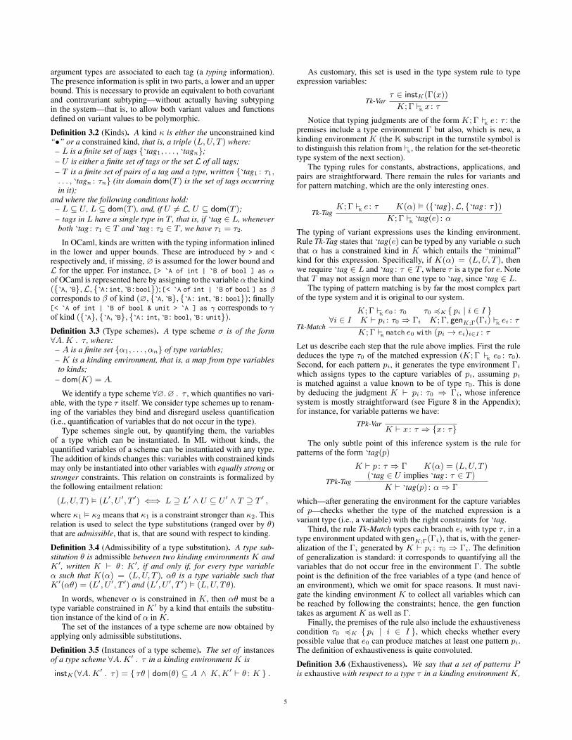
Definition 3.2 (Kinds). A kind κ is either the unconstrained kind“•” or a constrained kind, that is, a triple (L,U, T ) where:

– L is a finite set of tags tag1, . . . , tagn;– U is either a finite set of tags or the set L of all tags;– T is a finite set of pairs of a tag and a type, written tag1 : τ1,. . . , tagn : τn (its domain dom(T ) is the set of tags occurringin it);

and where the following conditions hold:– L ⊆ U , L ⊆ dom(T ), and, if U 6= L, U ⊆ dom(T );– tags in L have a single type in T , that is, if tag ∈ L, wheneverboth tag : τ1 ∈ T and tag : τ2 ∈ T , we have τ1 = τ2.

In OCaml, kinds are written with the typing information inlinedin the lower and upper bounds. These are introduced by > and <respectively and, if missing, ∅ is assumed for the lower bound andL for the upper. For instance, [> `A of int | `B of bool ] as αof OCaml is represented here by assigning to the variableα the kind( A, B,L, A : int, B : bool); [< `A of int | `B of bool ] as β

corresponds to β of kind (∅, A, B, A : int, B : bool); finally[< `A of int | `B of bool & unit > `A ] as γ corresponds to γof kind ( A, A, B, A : int, B : bool, B : unit).

Definition 3.3 (Type schemes). A type scheme σ is of the form∀A.K . τ , where:

– A is a finite set α1, . . . , αn of type variables;– K is a kinding environment, that is, a map from type variablesto kinds;

– dom(K) = A.

We identify a type scheme ∀∅.∅ . τ , which quantifies no vari-able, with the type τ itself. We consider type schemes up to renam-ing of the variables they bind and disregard useless quantification(i.e., quantification of variables that do not occur in the type).

Type schemes single out, by quantifying them, the variablesof a type which can be instantiated. In ML without kinds, thequantified variables of a scheme can be instantiated with any type.The addition of kinds changes this: variables with constrained kindsmay only be instantiated into other variables with equally strong orstronger constraints. This relation on constraints is formalized bythe following entailment relation:

(L,U, T ) (L′, U ′, T ′) ⇐⇒ L ⊇ L′ ∧ U ⊆ U ′ ∧ T ⊇ T ′ ,where κ1 κ2 means that κ1 is a constraint stronger than κ2. Thisrelation is used to select the type substitutions (ranged over by θ)that are admissible, that is, that are sound with respect to kinding.

Definition 3.4 (Admissibility of a type substitution). A type sub-stitution θ is admissible between two kinding environments K andK′, written K ` θ : K′, if and only if, for every type variableα such that K(α) = (L,U, T ), αθ is a type variable such thatK′(αθ) = (L′, U ′, T ′) and (L′, U ′, T ′) (L,U, Tθ).

In words, whenever α is constrained in K, then αθ must be atype variable constrained in K′ by a kind that entails the substitu-tion instance of the kind of α in K.

The set of the instances of a type scheme are now obtained byapplying only admissible substitutions.

Definition 3.5 (Instances of a type scheme). The set of instancesof a type scheme ∀A.K′ . τ in a kinding environment K is

instK(∀A.K′ . τ) = τθ | dom(θ) ⊆ A ∧ K,K′ ` θ : K .

As customary, this set is used in the type system rule to typeexpression variables:

Tk-Varτ ∈ instK(Γ(x))

K; ΓKx : τ

Notice that typing judgments are of the form K; ΓKe : τ : the

premises include a type environment Γ but also, which is new, akinding environment K (the K subscript in the turnstile symbol isto distinguish this relation from

S, the relation for the set-theoretic

type system of the next section).The typing rules for constants, abstractions, applications, and

pairs are straightforward. There remain the rules for variants andfor pattern matching, which are the only interesting ones.

Tk-TagK; Γ

Ke : τ K(α) ( tag,L, tag : τ)

K; ΓK

tag(e) : α

The typing of variant expressions uses the kinding environment.Rule Tk-Tag states that tag(e) can be typed by any variable α suchthat α has a constrained kind in K which entails the “minimal”kind for this expression. Specifically, if K(α) = (L,U, T ), thenwe require tag ∈ L and tag : τ ∈ T , where τ is a type for e. Notethat T may not assign more than one type to tag, since tag ∈ L.

The typing of pattern matching is by far the most complex partof the type system and it is original to our system.

Tk-Match

K; ΓKe0 : τ0 τ0 4K pi | i ∈ I

∀i ∈ I K ` pi : τ0 ⇒ Γi K; Γ, genK;Γ(Γi) Kei : τ

K; ΓKmatch e0 with (pi → ei)i∈I : τ

Let us describe each step that the rule above implies. First the rulededuces the type τ0 of the matched expression (K; Γ

Ke0 : τ0).

Second, for each pattern pi, it generates the type environment Γiwhich assigns types to the capture variables of pi, assuming piis matched against a value known to be of type τ0. This is doneby deducing the judgment K ` pi : τ0 ⇒ Γi, whose inferencesystem is mostly straightforward (see Figure 8 in the Appendix);for instance, for variable patterns we have:

TPk-VarK ` x : τ ⇒ x : τ

The only subtle point of this inference system is the rule forpatterns of the form tag(p)

TPk-Tag

K ` p : τ ⇒ Γ K(α) = (L,U, T )( tag ∈ U implies tag : τ ∈ T )

K ` tag(p) : α⇒ Γ

which—after generating the environment for the capture variablesof p—checks whether the type of the matched expression is avariant type (i.e., a variable) with the right constraints for tag.

Third, the rule Tk-Match types each branch ei with type τ , in atype environment updated with genK;Γ(Γi), that is, with the gener-alization of the Γi generated by K ` pi : τ0 ⇒ Γi. The definitionof generalization is standard: it corresponds to quantifying all thevariables that do not occur free in the environment Γ. The subtlepoint is the definition of the free variables of a type (and hence ofan environment), which we omit for space reasons. It must navi-gate the kinding environment K to collect all variables which canbe reached by following the constraints; hence, the gen functiontakes as argument K as well as Γ.

Finally, the premises of the rule also include the exhaustivenesscondition τ0 4K pi | i ∈ I , which checks whether everypossible value that e0 can produce matches at least one pattern pi.The definition of exhaustiveness is quite convoluted.

Definition 3.6 (Exhaustiveness). We say that a set of patterns Pis exhaustive with respect to a type τ in a kinding environment K,

5

and we write τ 4K P , when, for every K′, θ, and v,

(K ` θ : K′ ∧K′;∅Kv : τθ) =⇒ ∃p ∈ P, ς. v/p = ς .

In words, P is exhaustive when every value that can be typedwith any admissible substitution of τ is accepted by at least onepattern in P . OCaml does not impose exhaustiveness—it just sig-nals non-exhaustiveness with a warning—but our system does. Wedo so in order to have a simpler statement for soundness and to fa-cilitate the comparison with the system of the next section. We donot discuss how exhaustiveness can be effectively computed; formore information on how OCaml checks it, see Garrigue (2004)and Maranget (2007).

We conclude this section by stating the type soundness propertyof the K type system.

Theorem 3.1 (Progress). Let e be a well-typed, closed expression.Then, either e is a value or there exists an expression e′ such thate e′.

Theorem 3.2 (Subject reduction). Let e be an expression and τ atype such that K; Γ

Ke : τ . If e e′, then K; Γ

Ke′ : τ .

Corollary 3.3 (Type soundness). Let e be a well-typed, closedexpression, that is, such that K;∅

Ke : τ holds for some τ . Then,

either e diverges or it reduces to a value v such that K;∅Kv : τ .

4. Typing variants with set-theoretic typesWe now describe S, a type system for the language of Section 2based on set-theoretic types. The approach we take in its design isdrastically different from that followed for K. Rather than addinga kinding system to record information that types cannot express,we directly enrich the syntax of types so they can express all thenotions we need. Moreover, we add subtyping—using a semanticdefinition—rather than encoding it via instantiation. We exploittype connectives and subtyping to represent variant types as unionsand to encode bounded quantification by union and intersection.

We argue that S has several advantages with respect to the pre-vious system. It is more expressive: it is able to type some programsthat K rejects though they are actually type safe, and it can derivemore precise types than K. It is arguably a simpler formalization:typing works much like in ML except for the addition of subtyp-ing, we have explicit types for variants, and we can type patternmatching precisely and straightforwardly. Indeed, as regards pat-tern matching, an advantage of the S system is that it can expressexhaustiveness and non-redundancy checking as subtyping checks,while they cannot be expressed at the level of types in K.

Naturally, subtyping brings its own complications. We do notdiscuss its definition here, since we reuse the relation defined byCastagna and Xu (2011). The use of semantic subtyping makesthe definition of a typing algorithm challenging: Castagna et al.(2014, 2015) show how to define one in an explicitly-typed setting.Conversely, we study here an implicitly-typed language and hencestudy the problem of type reconstruction (in the next section).

While this system is based on that described by Castagna et al.(2014, 2015), there are significant differences which we discuss inSection 7. Notably, intersection types play a more limited role inour system (no rule allows the derivation of an intersection of arrowtypes for a function), making our type reconstruction complete.

4.1 Types and subtypingAs before, we consider a set V of type variables (ranged over by α,β, γ, . . . ) and the sets C, L, and B of language constants, tags, andbasic types (ranged over by c, tag, and b respectively).

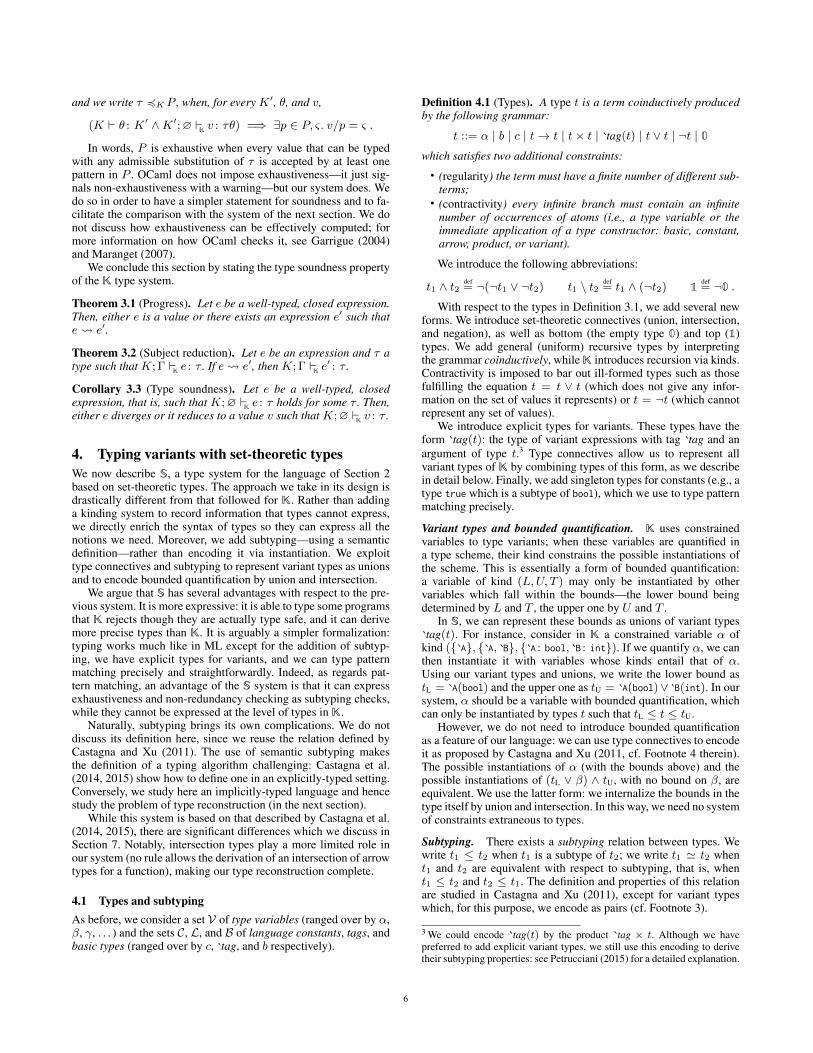
Definition 4.1 (Types). A type t is a term coinductively producedby the following grammar:

t ::= α | b | c | t→ t | t× t | tag(t) | t ∨ t | ¬t | 0which satisfies two additional constraints:

• (regularity) the term must have a finite number of different sub-terms;

• (contractivity) every infinite branch must contain an infinitenumber of occurrences of atoms (i.e., a type variable or theimmediate application of a type constructor: basic, constant,arrow, product, or variant).

We introduce the following abbreviations:

t1 ∧ t2def= ¬(¬t1 ∨ ¬t2) t1 \ t2

def= t1 ∧ (¬t2) 1

def= ¬0 .

With respect to the types in Definition 3.1, we add several newforms. We introduce set-theoretic connectives (union, intersection,and negation), as well as bottom (the empty type 0) and top (1)types. We add general (uniform) recursive types by interpretingthe grammar coinductively, while K introduces recursion via kinds.Contractivity is imposed to bar out ill-formed types such as thosefulfilling the equation t = t ∨ t (which does not give any infor-mation on the set of values it represents) or t = ¬t (which cannotrepresent any set of values).

We introduce explicit types for variants. These types have theform tag(t): the type of variant expressions with tag tag and anargument of type t.3 Type connectives allow us to represent allvariant types of K by combining types of this form, as we describein detail below. Finally, we add singleton types for constants (e.g., atype true which is a subtype of bool), which we use to type patternmatching precisely.

Variant types and bounded quantification. K uses constrainedvariables to type variants; when these variables are quantified ina type scheme, their kind constrains the possible instantiations ofthe scheme. This is essentially a form of bounded quantification:a variable of kind (L,U, T ) may only be instantiated by othervariables which fall within the bounds—the lower bound beingdetermined by L and T , the upper one by U and T .

In S, we can represent these bounds as unions of variant typestag(t). For instance, consider in K a constrained variable α of

kind ( A, A, B, A : bool, B : int). If we quantify α, we canthen instantiate it with variables whose kinds entail that of α.Using our variant types and unions, we write the lower bound astL = A(bool) and the upper one as tU = A(bool)∨ B(int). In oursystem, α should be a variable with bounded quantification, whichcan only be instantiated by types t such that tL ≤ t ≤ tU.

However, we do not need to introduce bounded quantificationas a feature of our language: we can use type connectives to encodeit as proposed by Castagna and Xu (2011, cf. Footnote 4 therein).The possible instantiations of α (with the bounds above) and thepossible instantiations of (tL ∨ β) ∧ tU, with no bound on β, areequivalent. We use the latter form: we internalize the bounds in thetype itself by union and intersection. In this way, we need no systemof constraints extraneous to types.

Subtyping. There exists a subtyping relation between types. Wewrite t1 ≤ t2 when t1 is a subtype of t2; we write t1 ' t2 whent1 and t2 are equivalent with respect to subtyping, that is, whent1 ≤ t2 and t2 ≤ t1. The definition and properties of this relationare studied in Castagna and Xu (2011), except for variant typeswhich, for this purpose, we encode as pairs (cf. Footnote 3).

3 We could encode tag(t) by the product tag × t. Although we havepreferred to add explicit variant types, we still use this encoding to derivetheir subtyping properties: see Petrucciani (2015) for a detailed explanation.

6

Ts-Vart ∈ inst(Γ(x))

ΓSx : t

Ts-ConstΓ

Sc : c

Ts-AbstrΓ, x : t1 S

e : t2

ΓSλx. e : t1 → t2

Ts-ApplΓ

Se1 : t′ → t Γ

Se2 : t′

ΓSe1 e2 : t

Ts-PairΓ

Se1 : t1 Γ

Se2 : t2

ΓS

(e1, e2) : t1 × t2Ts-Tag

ΓSe : t

ΓS

tag(e) : tag(t)

Ts-Match

ΓSe0 : t0 t0 ≤

∨i∈I*pi+ ti = (t0 \

∨j<i*pj+) ∧ *pi+

∀i ∈ I Γ, genΓ(ti//pi) Sei : t

′i

ΓSmatch e0 with (pi → ei)i∈I :

∨i∈I t

′i

Ts-SubsumΓ

Se : t′ t′ ≤ tΓ

Se : t

Figure 2. Typing relation of the S type system.

In brief, subtyping is given a semantic definition, in the sensethat t1 ≤ t2 holds if and only if Jt1K ⊆ Jt2K, where J·K is an in-terpretation function mapping types to sets of elements from somedomain (intuitively, the set of values of the language). The inter-pretation is “set-theoretic” as it interprets union types as unions,negation as complementation, and products as Cartesian products.

In general, in the semantic-subtyping approach, we consider atype to denote the set of all values that have that type (we will saythat some type “is” the set of values of that type). In particular, forarrow types, the type t1 → t2 is that of function values (i.e., λ-abstractions) which, if they are given an argument in Jt1K and theydo not diverge, yield a result in Jt2K. Hence, all types of the form0→ t, for any t, are equivalent (as only diverging expressions canhave type 0): any of them is the type of all functions. Conversely,1 → 0 is the type of functions that (provably) diverge on allinputs: a function of this type should yield a value in the emptytype whenever it terminates, and that is impossible.

The presence of variables complicates the definition of semanticsubtyping. Here, we just recall from Castagna and Xu (2011) thatsubtyping is preserved by type substitutions: t1 ≤ t2 impliest1θ ≤ t2θ for every type substitution θ.

4.2 Type systemWe present S focusing on the differences with respect to the systemof OCaml (i.e., K); full definitions are in the Appendix. Unlike inK, type schemes here are defined just as in ML as we no longerneed kinding constraints.

Definition 4.2 (Type schemes). A type scheme s is of the form∀A. t, where A is a finite set α1, . . . , αn of type variables.

As in K, we identify a type scheme ∀∅. t with the type t itself,we consider type schemes up to renaming of the variables theybind, and we disregard useless quantification.

We write var(t) for the set of type variables occurring in a typet; we say they are the free variables of t, and we say that t is groundor closed if and only if var(t) is empty. The (coinductive) definitionof var can be found in Castagna et al. (2014, Definition A.2).

Unlike in ML, types in our system can contain variables whichare irrelevant to the meaning of the type. For instance, α × 0 isequivalent to 0 (with respect to subtyping), as we interpret producttypes into Cartesian products. Thus, α is irrelevant in α × 0.To capture this concept, we introduce the notion of meaningfulvariables in a type t. We define these to be the set

mvar(t) = α ∈ var(t) | t[0/α] 6' t ,

where the choice of 0 to replace α is arbitrary (any other closedtype yields the same definition). Equivalent types have exactlythe same meaningful variables. To define generalization, we allowquantifying variables which are free in the type environment but are

meaningless in it (intuitively, we act as if types were in a canonicalform without irrelevant variables).

We extend var to type schemes as var(∀A. t) = var(t) \A, anddo likewise for mvar.

Type substitutions are defined in a standard way by coinduction;there being no kinding system, we do not need the admissibilitycondition of K.

We define type environments Γ as usual. The operations of gen-eralization of types and instantiation of type schemes, instead, mustaccount for the presence of irrelevant variables and of subtyping.

Generalization with respect to Γ quantifies all variables in a typeexcept for those that are free and meaningful in Γ:

genΓ(t) = ∀A. t , where A = var(t) \mvar(Γ) .

We extend gen pointwise to sets of bindings x1 : t1, . . . , xn : tn.The set of instances of a type scheme is given by

inst(∀A. t) = tθ | dom(θ) ⊆ A ,

and we say that a type scheme s1 is more general than a typescheme s2—written s1 v s2—if

∀t2 ∈ inst(s2). ∃t1 ∈ inst(s1). t1 ≤ t2 . (1)

Notice that the use of subtyping in the definition above general-izes the corresponding definition of ML (which uses equality) andsubsumes the notion of “admissibility” of K by a far simpler andmore natural relation (cf. Definitions 3.4 and 3.5).

Figure 2 defines the typing relation ΓSe : t of the S type

system (we use the S subscript in the turnstile symbol to distinguishthis relation from that for K). All rules except that for patternmatching are straightforward. Note that Ts-Const is more precisethan in K since we have singleton types, and that Ts-Tag uses thetypes we have introduced for variants.

The rule Ts-Match involves two new concepts that we presentbelow. We start by typing the expression to be matched, e0, withsome type t0. We also require every branch ei to be well-typed withsome type t′i: the type of the whole match expression is the union ofall t′i. We type each branch in an environment expanded with typesfor the capture variables of pi: this environment is generated by thefunction ti//pi (described below) and is generalized.

The advantage of our richer types here is that, given any pattern,the set of values it accepts is always described precisely by a type.

Definition 4.3 (Accepted type). The accepted type *p+ of a patternp is defined inductively as:

* + = *x+ = 1 *c+ = c

*(p1, p2)+ = *p1+× *p2+ * tag(p)+ = tag(*p+)

*p1&p2+ = *p1+ ∧ *p2+ *p1|p2+ = *p1+ ∨ *p2+ .

For well-typed values v, we have v/p 6= Ω ⇐⇒ ∅Sv : *p+.

We use accepted types to express the condition of exhaustiveness:

7

JαKK =

α if K(α) = •(lowK(L, T ) ∨ α) ∧ uppK(U, T ) if K(α) = (L,U, T )

JbKK = b

Jτ1 → τ2KK = Jτ1KK → Jτ2KKJτ1 × τ2KK = Jτ1KK × Jτ2KK

where: lowK(L, T ) =∨

tag∈L tag(∧

tag : τ∈T JτKK)

uppK(U, T ) =

∨tag∈U tag(

∧tag : τ∈T JτKK) if U 6= L∨

tag∈dom(T ) tag(∧

tag : τ∈T JτKK) ∨ (1V \∨

tag∈dom(T ) tag(1)) if U = L

Figure 3. Translation of k-types to s-types.

t0 ≤∨i∈I*pi+ ensures that every value e0 can reduce to (i.e., every

value in t0) will match at least one pattern (i.e., is in the acceptedtype of some pattern). We also use them to compute precisely thesubtypes of t0 corresponding to the values which will trigger eachbranch. In the rule, ti is the type of all values which will be selectedby the i-th branch: those in t0 (i.e., generated by e0), not in any*pj+ for j < i (i.e., not captured by any previous pattern), and in*pi+ (i.e., accepted by pi). These types ti allow us to express non-redundancy checks: if ti ≤ 0 for some i, then the correspondingpattern will never be selected (which likely means the programmerhas made some mistake and should receive a warning).4

The last element we must describe is the generation of types forthe capture variables of each pattern by the ti//pi function. Here,our use of ti means we exploit the shape of the pattern pi and of theprevious ones to generate more precise types; environment genera-tion in K essentially uses only t0 and is therefore less precise.

Environment generation relies on two functions π1 and π2

which extract the first and second component of a type t ≤ 1× 1.For instance, if t = (α×β)∨(bool×int), we have π1(t) = α∨booland π2(t) = β ∨ int. Given any tag tag, π tag does likewise forvariant types with that tag. See Castagna et al. (2014, AppendixC.2.1) and Petrucciani (2015) for the full details.

Definition 4.4 (Pattern environment generation). Given a pattern pand a type t ≤ *p+, the type environment t//p generated by patternmatching is defined inductively as:

t// = ∅ t//(p1, p2) = π1(t)//p1 ∪ π2(t)//p2

t//x = x : t t// tag(p) = π tag(t)//p

t//c = ∅ t//p1&p2 = t//p1 ∪ t//p2

t//p1|p2 = (t ∧ *p1+)//p1 ∨∨ (t \ *p1+)//p2

where (Γ ∨∨ Γ′)(x) = Γ(x) ∨ Γ′(x).

The S type system is sound, as stated by the following properties.

Theorem 4.1 (Progress). Let e be a well-typed, closed expression(i.e., ∅

Se : t holds for some t). Then, either e is a value or there

exists an expression e′ such that e e′.

Theorem 4.2 (Subject reduction). Let e be an expression and t atype such that Γ

Se : t. If e e′, then Γ

Se′ : t.

Corollary 4.3 (Type soundness). Let e be a well-typed, closedexpression, that is, such that ∅

Se : t holds for some t. Then,

either e diverges or it reduces to a value v such that ∅Sv : t.

4 We can also exploit redundancy information to exclude certain branchesfrom typing (see Section 6.1), though it is not always possible during typereconstruction.

4.3 Comparison with K

Our type system S extends K in the sense that every well-typedprogram of K is also well-typed in S: we say that S is completewith respect to K.

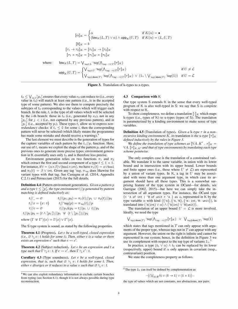
To show completeness, we define a translation J·KK which mapsk-types (i.e., types of K) to s-types (types of S). The translationis parameterized by a kinding environment to make sense of typevariables.

Definition 4.5 (Translation of types). Given a k-type τ in a non-recursive kinding environment K, its translation is the s-type JτKKdefined inductively by the rules in Figure 3.

We define the translation of type schemes as J∀A.K′ . τKK =∀A. JτKK,K′ and that of type environments by translating each typescheme pointwise.

The only complex case is the translation of a constrained vari-able. We translate it to the same variable, in union with its lowerbound and in intersection with its upper bound. Lower boundsand finite upper ones (i.e., those where U 6= L) are representedby a union of variant types. In K, a tag in U may be associ-ated with more than one argument type, in which case its ar-gument should have all these types. This is a somewhat sur-prising feature of the type system in OCaml—for details, seeGarrigue (2002, 2015)—but here we can simply take the in-tersection of all argument types. For instance, the OCaml type[< `A of int | `B of unit > `A ] as α, represented in K by thetype variable α with kind ( A, A, B, A : int, B : unit), istranslated into ( A(int) ∨ α) ∧ ( A(int) ∨ B(unit)).

The translation of an upper bound U = L is more involved.Ideally, we need the type∨

tag∈dom(T ) tag(∧

tag : τ∈T JτKK) ∨∨

tag/∈dom(T ) tag(1)

which states that tags mentioned in T can only appear with argu-ments of the proper type, whereas tags not in T can appear with anyargument. However, the union on the right is infinite and cannot berepresented in our system; hence, in the definition in Figure 3 weuse its complement with respect to the top type of variants 1V.5

In practice, a type (tL ∨ α) ∧ tU can be replaced by its lower(respectively, upper) bound if α only appears in covariant (resp.,contravariant) position.

We state the completeness property as follows.

5 The type 1V can itself be defined by complementation as

¬((∨b∈B b) ∨ (0→ 1) ∨ (1× 1)

):

the type of values which are not constants, nor abstractions, nor pairs.

8

TRs-Varx : t⇒ x ≤ t

TRs-Constc : t⇒ c ≤ t

TRs-Abstre : β ⇒ C

λx. e : t⇒ def x : α in C, α→ β ≤ t

TRs-Apple1 : α→ β ⇒ C1 e2 : α⇒ C2

e1 e2 : t⇒ C1 ∪ C2 ∪ β ≤ tTRs-Pair

e1 : α1 ⇒ C1 e2 : α2 ⇒ C2

(e1, e2) : t⇒ C1 ∪ C2 ∪ α1 × α2 ≤ t

TRs-Tage : α⇒ C

tag(e) : t⇒ C ∪ tag(α) ≤ tTRs-Match

e0 : α⇒ C0 ti = (α \∨j<i*pj+) ∧ *pi+

∀i ∈ I ti///pi ⇒ (Γi, Ci) ei : β ⇒ C′iC′0 = C0 ∪ (

⋃i∈I Ci) ∪ α ≤

∨i∈I*pi+

match e0 with (pi → ei)i∈I : t⇒ let [C′0](Γi in C′i)i∈I , β ≤ t

Figure 4. Constraint generation rules.

Theorem 4.4 (Preservation of typing). Let e be an expression, Ka non-recursive kinding environment, Γ a k-type environment, andτ a k-type. If K; Γ

Ke : τ , then JΓKK S

e : JτKK .

Notice that we have defined J·KK by induction. Therefore,strictly speaking, we have only proved that S deduces all the judg-ments provable for non-recursive types in K. Indeed, in the state-ment we require the kinding environment K to be non-recursive6.We conjecture that the result holds also with recursive kindings andthat it can be proven by coinductive techniques.

5. Type reconstructionIn this section, we study type reconstruction for the S type system.We build on the work of Castagna et al. (2015), who study localtype inference and type reconstruction for the polymorphic versionof CDuce. In particular, we reuse their work on the resolution ofthe tallying problem, which plays in our system the same role asunification in ML.

Our contribution is threefold: (i) we prove type reconstructionfor our system to be both sound and complete, while in Castagnaet al. (2015) it is only proven to be sound for CDuce (indeed,we rely on the restricted role of intersection types in our sys-tem to obtain this result); (ii) we describe reconstruction withlet-polymorphism and use structured constraints to separate con-straint generation from constraint solving; (iii) we define recon-struction for full pattern matching. Both let-polymorphism and pat-tern matching are omitted in Castagna et al. (2015).

Type reconstruction for a program (a closed expression) e con-sists in finding a type t such that ∅

Se : t can be derived: we see it

as finding a type substitution θ such that∅Se : αθ holds for some

fresh variable α. We generalize this to non-closed expressions andto reconstruction of types that are partially known. Thus, we saythat type reconstruction consists—given an expression e, a type en-vironment Γ, and a type t—in computing a type substitution θ suchthat Γθ

Se : tθ holds, if any such θ exists.

Reconstruction in our system proceeds in two main phases. Inthe first, constraint generation (Section 5.1), we generate froman expression e and a type t a set of constraints that record theconditions under which emay be given type t. In the second phase,constraint solving (Sections 5.2–5.3), we solve (if possible) theseconstraints to obtain a type substitution θ.

We keep these two phases separate following an approach in-spired by presentations of HM(X) (Pottier and Rémy 2005): weuse structured constraints which contain expression variables, sothat constraint generation does not depend on the type environmentΓ that e is to be typed in. Γ is used later for constraint solving.

6 We say K is non-recursive if it does not contain any cycle α, α1, . . . ,αn, α such that the kind of each variable αi contains αi+1.

Constraint solving is itself made up of two steps: constraintrewriting (Section 5.2) and type-constraint solving (Section 5.3).In the former, we convert a set of structured constraints into asimpler set of subtyping constraints. In the latter, we solve thisset of subtyping constraints to obtain a set of type substitutions;this latter step is analogous to unification in ML and is computedusing the tallying algorithm of Castagna et al. (2015). Constraintrewriting also uses type-constraint solving internally; hence, thesetwo steps are actually intertwined in practice.

5.1 Constraint generationGiven an expression e and a type t, constraint generation computesa finite set of constraints of the form defined below.

Definition 5.1 (Constraints). A constraint c is a term inductivelygenerated by the following grammar:

c ::= t ≤ t | x ≤ t | def Γ in C | let [C](Γi in Ci)i∈I

where C ranges over constraint sets, that is, finite sets of con-straints, and where the range of every type environment Γ in con-straints of the form def or let only contains types (i.e., trivial typeschemes).

A constraint of the form t ≤ t′ requires tθ ≤ t′θ to hold for thefinal substitution θ. One of the form x ≤ t constrains the type of x(actually, an instantiation of its type scheme with fresh variables)in the same way. A definition constraint defΓ in C introduces newexpression variables, as we do in abstractions; these variables maythen occur in C. We use def constraints to introduce monomorphicbindings (environments with types and not type schemes).

Finally, let constraints introduce polymorphic bindings. We usethem for pattern matching: hence, we define them with multiplebranches (the constraint sets Ci’s), each with its own environment(binding the capture variables of each pattern to types). To solvea constraint let [C0](Γi in Ci)i∈I , we first solve C0 to obtaina substitution θ; then, we apply θ to all types in each Γi and wegeneralize the resulting types; finally, we solve each Ci (in anenvironment expanded with the generalization of Γiθ).

We define constraint generation as a relation e : t ⇒ C, givenby the rules in Figure 4. We assume all variables introduced bythe rules to be fresh (see the Appendix for the formal treatment offreshness: cf. Definition A.39 and Figures 13 and 14). Constraintgeneration for variables and constants (rules TRs-Var and TRs-Const) just yields a subtyping constraint. For an abstraction λx. e(rule TRs-Abstr), we generate constraints for the body and wrapthem into a definition constraint binding x to a fresh variable α;we add a subtyping constraint to ensure that λx. e has type t bysubsumption. The rules for applications, pairs, and tags are similar.

For pattern-matching expressions (rule TRs-Match), we use anauxiliary relation t///p ⇒ (Γ, C) to generate the pattern type

9

∀i ∈ I Γ ` ci Di

Γ ` ci | i ∈ I ⋃i∈I Di Γ ` t ≤ t′ t ≤ t′

Γ(x) = ∀α1, . . . , αn. txΓ ` x ≤ t tx[β1/α1, . . . , βn/αn] ≤ t

Γ,Γ′ ` C D

Γ ` def Γ′ in C D

Γ ` C0 D0 θ0 ∈ tally(D0)∀i ∈ I Γ, genΓθ0

(Γiθ0) ` Ci Di

Γ ` let [C0](Γi in Ci)i∈I equiv(θ0) ∪⋃i∈I Di

Figure 5. Constraint rewriting rules.

environment Γ, together with a set of constraints C in case theenvironment contains new type variables. The full definition is inthe Appendix; as an excerpt, consider the rules for variable and tagpatterns.

t///x⇒ (x : t,∅)

α///p⇒ (Γ, C)

t/// tag(p)⇒ (Γ, C ∪ t ≤ tag(α))

The rule for variable patterns produces no constraints (and theempty environment). Conversely, the rule for tags must introducea new variable α to stand for the argument type: the constraintproduced mirrors the use of the projection operator π tag in thedeductive system. To generate constraints for a pattern-matchingexpression, we generate them for the expression to be matchedand for each branch separately. All these are combined in a letconstraint, together with the constraints generated by patterns andwith α ≤

∨i∈I *pi+, which ensures exhaustiveness.

5.2 Constraint rewritingThe first step of constraint solving consists in rewriting the con-straint set into a simpler form that contains only subtyping con-straints, that is, into a set of the form t1 ≤ t′1, . . . , tn ≤ t′n(i.e., no let, def, or expression variables). We call such sets type-constraint sets (ranged over by D).

Constraint rewriting is defined as a relation Γ ` C D:between type environments, constraints or constraint sets, and type-constraint sets. It is given by the rules in Figure 5.

We rewrite constraint sets pointwise. We leave subtyping con-straints unchanged. In variable type constraints, we replace the vari-able x with an instantiation of the type scheme Γ(x) with the vari-ables β1, . . . , βn, which we assume to be fresh. We rewrite defconstraints by expanding the environment and rewriting the innerconstraint set.

The complex case is that of let constraints, which is whererewriting already performs type-constraint solving. We first rewritethe constraint set C0. Then we extract a solution θ0—if anyexists—by the tally algorithm (described below). The algorithmcan produce multiple alternative solutions: hence, this step is non-deterministic. Finally, we rewrite each of the Ci in an expandedenvironment. We perform generalization, so let constraints mayintroduce polymorphic bindings. The resulting type-constraint setis the union of the type-constraint sets obtained for each branchplus equiv(θ0), which is defined as

equiv(θ0) =⋃α∈dom(θ0)α ≤ αθ0, αθ0 ≤ α .

We add the constraints of equiv(θ0) because tallying mightgenerate multiple incompatible solutions for the constraints in D0.The choice of θ0 is arbitrary, but we must force subsequent steps ofconstraint solving to abide by it. Adding equiv(θ0) ensures thatevery solution θ to the resulting type-constraint set will satisfyαθ ' αθ0θ for every α, and hence will not contradict our choice.

5.3 Type-constraint solvingCastagna et al. (2015) define the tallying problem as the problem—in our terminology—of finding a substitution that satisfies a giventype-constraint set.

Definition 5.2. We say that a type substitution θ satisfies a type-constraint set D, written θ D, if tθ ≤ t′θ holds for every t ≤ t′in D. When θ satisfies D, we say it is a solution to the tallyingproblem of D.

The tallying problem is the analogue in our system of the uni-fication problem in ML. However, there is a very significant dif-ference: while unification admits principal solutions, tallying doesnot. Indeed, the algorithm to solve the tallying problem for a type-constraint set produces a finite set of type substitutions. The algo-rithm is sound in that all substitutions it generates are solutions. Itis complete in the sense that any other solution is less general thanone of those in the set: we have a finite number of solutions whichare principal when taken together, but not necessarily a single so-lution that is principal on its own.

This is a consequence of our semantic definition of subtyp-ing. As an example, consider subtyping for product types: with astraightforward syntactic definition, a constraint t1 × t′1 ≤ t2 × t′2would simplify to the conjunction of two constraints t1 ≤ t2 andt′1 ≤ t′2. With semantic subtyping—where products are seen asCartesian products—that simplification is sound, but it is not theonly possible choice: either t1 ≤ 0 or t′1 ≤ 0 is also enough toensure t1 × t′1 ≤ t2 × t′2, since both ensure t1 × t′1 ' 0. The threepossible choices can produce incomparable solutions.

Castagna et al. (2015, Section 3.2 and Appendix C.1) define asound, complete, and terminating algorithm to solve the tallyingproblem, which can be adapted to our types by encoding variantsas pairs. We refer to this algorithm here as tally (it is Sol∅ in thereferenced work) and state its properties.

Property 5.3 (Tallying algorithm). There exists a terminating al-gorithm tally such that, for any type-constraint set D, tally(D) isa finite, possibly empty, set of type substitutions.

Theorem 5.1 (Soundness and completeness of tally). Let D be atype-constraint set. For any type substitution θ:

– if θ ∈ tally(D), then θ D;– if θ D, then ∃θ′ ∈ tally(D), θ′′.∀α ∈ dom(θ).αθ ' αθ′θ′′.

Hence, given a type-constraint set, we can use tally to either finda set of solutions or determine it has no solution: tally(D) = ∅occurs if and only if there exists no θ such that θ D.

5.3.1 Properties of type reconstructionType reconstruction as a whole consists in generating a constraintset C from an expression, rewriting this set into a type-constraintset D (which can require solving intermediate type-constraint sets)and finally solvingD by the tally algorithm. Type reconstruction isboth sound and complete with respect to the deductive type systemS. We state these properties in terms of constraint rewriting.

10

Theorem 5.2 (Soundness of constraint generation and rewriting).Let e be an expression, t a type, and Γ a type environment. Ife : t⇒ C, Γ ` C D, and θ D, then Γθ

Se : tθ.

Theorem 5.3 (Completeness of constraint generation and rewrit-ing). Let e be an expression, t a type, and Γ a type environment.Let θ be a type substitution such that Γθ

Se : tθ.

Let e : t ⇒ C. There exist a type-constraint set D and atype substitution θ′, with dom(θ) ∩ dom(θ′) = ∅, such thatΓ ` C D and (θ ∪ θ′) D.

These theorems and the properties above express soundness andcompleteness for the reconstruction system. Decidability is a directconsequence of the termination of the tallying algorithm.

5.3.2 Practical issuesAs compared to reconstruction in ML, our system has the disad-vantage of being non-deterministic: in practice, an implementationshould check every solution that tallying generates at each stepof type-constraint solving until it finds a choice of solution whichmakes the whole program well-typed. This should be done at ev-ery step of generalization (that is, for every match expression) andmight cripple efficiency. Whether this is significant in practice ornot is a question that requires further study and experimentation.Testing multiple solutions cannot be avoided since our system doesnot admit principal types. For instance the function

let f(x,y) = (function (`A,`A)|(`B,`B)→`C)(x,y)

has both type (`A,`A)→`C and type (`B,`B)→`C (and neither isbetter than the other) but it is not possible to deduce for it their leastupper bound (`A,`A)∨(`B,`B)→`C (which would be principal).

Multiple solutions often arise by instantiating some type vari-ables by the empty type. Such solutions are in many cases sub-sumed by other more general solutions, but not always. For in-stance, consider the α list data-type (encoded as the recursivetype X = (α,X)∨[]) together with the classic map function overlists (the type of which is (α→ β)→α list→β list). The appli-cation of map to the successor function succ : int→ int has typeint list→ int list, but also type []→ [] (obtained by instantiat-ing all the variables of the type of map by the empty type). Thelatter type is correct, cannot be derived (by instantiation and/orsubtyping) from the former, but it is seldom useful (it just statesthat map(succ) maps the empty list into the empty list). As such, itshould be possible to define some preferred choice of solution (i.e.,the solution that does not involve empty types) which is likely to bethe most useful in practice. As it happens, we would like to try torestrict the system so that it only considers solutions without emptytypes. While it would make us lose completeness with respect to S,it would be interesting to compare the restricted system with ML(with respect to which it could still be complete).

6. ExtensionsIn this section, we present three extensions or modifications to theS type system; the presentation is just sketched for space reasons:the details of all three can be found in the Appendix.

The first is the introduction of overloaded functions typed viaintersection types, as done in CDuce. The second is a refinementof the typing of pattern matching, which we have shown as partof Example 2 (the function g and our definition of map). Finally,the third is a restriction of our system to adapt it to the semanticsof the OCaml implementation which, unlike our calculus, cannotcompare safely untagged values of different types at runtime.

6.1 Overloaded functionsCDuce allows the use of intersection types to type overloadedfunctions precisely: for example, it can type the negation function

notdef= λx. match x with true→ false | false→ true

with the type (true → false) ∧ (false → true), which is moreprecise than bool→ bool. We can add this feature by changing therule to type λ-abstractions to

∀j ∈ J. Γ, x : t′j ` e : tj

Γ ` λx. e :∧j∈J t

′j → tj

which types the abstraction with an intersection of arrow types,provided each of them can be derived for it. The rule above roughlycorresponds to the one introduced by Reynolds for the languageForsythe (Reynolds 1997). With this rule alone, however, one hasonly the so-called coherent overloading (Pierce 1991), that is, thepossibility of assigning different types to the same piece of code,yielding an intersection type. In full-fledged overloading, instead,different pieces of code are executed for different types of the input.This possibility was first introduced by CDuce (Frisch et al. 2002;Benzaken et al. 2003) and it is obtained by typing pattern matchingwithout taking into account the type of the branches that cannot beselected for a given input type. Indeed, the function “not” abovecannot be given the type we want if we just add the rule above: itcan neither be typed as true→ false nor as false→ true.

To use intersections effectively for pattern matching, we needto exclude redundant patterns from typing. We do so by changingthe rule Ts-Match (in Figure 2): when for some branch i we haveti ≤ 0, we do not type that branch at all, and we do not considerit in the result type (that is, we set t′i = 0). In this way, if we taket′j = true, we can derive tj = false (and vice versa). Indeed, ifwe assume that the argument is true, the second branch will neverbe selected: it is therefore sound not to type it at all. This typingtechnique is peculiar to CDuce’s overloading. However, functionsin CDuce are explicitly typed. As type reconstruction is undecid-able for unrestricted intersection type systems, this extension wouldmake annotations necessary in our system as well. We plan to studythe extension of our system with intersection types for functionsand to adapt reconstruction to also consider explicit annotations.

6.2 Refining the type of expressions in pattern matchingTwo of our motivating examples concerning pattern matching(from Section 1, Example 2) involved a refinement of the typing ofpattern matching that we have not described yet, but which can beadded as a small extension of our S system.

Recall the function g defined as λx. match x with A →id2 x | → x, where id2 has domain A ∨ B. Like OCaml, Srequires the type of x to be a subtype of A ∨ B, but this constraintis unnecessary because id2 x is only computed when x = A. Tocapture this, we need pattern matching to introduce more precisetypes for variables in the matched expression; this is a form ofoccurrence typing (Tobin-Hochstadt and Felleisen 2010) or flowtyping (Pearce 2013).

We first consider pattern matching on a variable. In an expres-sion matchx with (pi → ei)i∈I we can obtain this increased preci-sion by using the type ti—actually, its generalization—for x whiletyping the i-th branch. In the case of g, the first branch is typed as-suming x has type t0 ∧ A, where t0 is the type we have derived forx. As a result, the constraint t0 ∧ A ≤ A ∨ B does not restrict t0.

We can express this so as to reuse pattern environment genera-tion. Let L·M : E → P be a function such that LxM = x and LeM =when e is not a variable. Then, we obtain the typing above if weuse

Γ, genΓ(ti//Le0M), genΓ(ti//pi)

as the type environment in which we type the i-th branch, ratherthan Γ, genΓ(ti//pi).

We generalize this approach to refine types also for variablesoccurring inside pairs and variants. To do so, we redefine L·M.

11

On variants, we let L tag(e)M = tag(LeM). On pairs, ideally wewant L(e1, e2)M = (Le1M, Le2M): however, pair patterns cannot haverepeated variables, while (e1, e2) might. We therefore introducea new form of pair pattern 〈p1, p2〉 (only for internal use) whichadmits repeated variables: environment generation for such patternsintersects the types it obtains for each occurrence of a variable.

6.3 Applicability to OCamlA thesis of this work is that the type system of OCaml—specifically,the part dealing with polymorphic variants and pattern matching—could be profitably replaced by an alternative, set-theoretic system.Of course, we need the set-theoretic system to be still type safe.

In Section 4, we stated that S is sound with respect to thesemantics we gave in Section 2. However, this semantics is notprecise enough, as it does not correspond to the behaviour of theOCaml implementation on ill-typed terms.7

Notably, OCaml does not record type information at runtime:values of different types cannot be compared safely and constantsof different basic types might have the same representation (as, forinstance, 1 and true). Consider as an example the two functions

λx. match x with true→ true | → false

λx. match x with (true, true)→ true | → false .

Both can be given the type 1 → bool in S, which is indeed safein our semantics. Hence, we can apply both of them to 1, andboth return false. In OCaml, conversely, the first would return trueand the second would cause a crash. The types bool → bool andbool×bool→ bool, respectively, would be safe for these functionsin OCaml.

To model OCaml more faithfully, we define an alternative se-mantics where matching a value v against a pattern p can have threeoutcomes rather than two: it can succeed (v/p = ς), fail (v/p =Ω), or be undefined (v/p = f). Matching is undefined wheneverit is unsafe in OCaml: for instance, 1/true = 1/(true, true) = f(see Appendix A.5.3 for the full definition).

We use the same definition as before for reduction (see Sec-tion 2.2). Note that a match expression on a value reduces to thefirst branch for which matching is successful if the result is Ω forall previous branches. If matching for a branch is undefined, nobranch after it can be selected; hence, there are fewer possible re-ductions with this semantics.

Adapting the type system requires us to restrict the typing ofpattern matching so that undefined results cannot arise. We definethe compatible type dpe of a pattern p as the type of values v whichcan be safely matched with it: those for which v/p 6= f. Forinstance, d1e = int. The rule for pattern matching should requirethat the type t0 of the matched expression be a subtype of all dpie.

Note that this restricts the use of union types in the system. Forinstance, if we have a value of type bool ∨ int, we can no longeruse pattern matching to discriminate between the two cases. This isto be expected in a language without runtime type tagging: indeed,union types are primarily used for variants, which reintroduce tag-ging explicitly. Nevertheless, having unions of non-variant types inthe system is still useful, both internally (to type pattern matching)and externally (see Example 3 in Section 1, for instance).

7. Related workWe discuss here the differences between our system and otherformalizations of variants in ML. We also compare our work withthe work on CDuce and other union/intersection type systems.

7 We can observe this if we bypass type-checking, for instance by usingObj.magic for unsafe type conversions.

7.1 Variants in ML: formal models and OCamlK is based on the framework of structural polymorphism and morespecifically on the presentations by Garrigue (2002, 2015). Thereexist several other systems with structural polymorphism: for in-stance, the earlier one by Garrigue (1998) or Ohori (1995) (whichGarrigue (2002, 2015) generalize) and more expressive constraint-based frameworks, like the presentation of HM(X) by Pottier andRémy (2005). We have chosen as a starting point the system whichcorresponds most closely to the actual implementation in OCaml.

With respect to the system in Garrigue (2002, 2015), K differsmainly in three respects. First, Garrigue’s system describes con-straints more abstractly and can accommodate different forms ofpolymorphic typing of variants and of records. We only considervariants and, as a result, give a more concrete presentation. Second,we model full pattern matching instead of “shallow” case analy-sis. To our knowledge, pattern matching on polymorphic variantsin OCaml is only treated in Garrigue (2004) and only as concernssome problems with type reconstruction. We have chosen to for-malize it to compare K to our set-theoretic type system S, whichadmits a simpler formalization and more precise typing. However,we have omitted a feature of OCaml that allows refinement of vari-ant types in alias patterns and which is modeled in Garrigue (2002)by a split construct. While this feature makes OCaml more pre-cise than K, it is subsumed in S by the precise typing of capturevariables. Third, we did not study type inference for K. Since Sis more expressive than K and since we describe complete recon-struction for it, extending Garrigue’s inference system to patternmatching was unnecessary for the goals of this work.

As compared to OCaml itself (or, more precisely, to the frag-ment we consider) our formalization is different because it requiresexhaustiveness; this might not always by practical in K, but non-exhaustive pattern matching is no longer useful once we introducemore precise types, as in S. Other differences include not consider-ing variant refinement in alias patterns, as noted above, and the han-dling of conjunctive types, where OCaml is more restrictive thanwe are in order to infer more intuitive types (as discussed in Gar-rigue 2004, Section 4.1).

7.2 S and the CDuce calculusS reuses the subtyping relation defined by Castagna and Xu (2011)and some of the work described in Castagna et al. (2014, 2015) (no-tably, the encoding of bounded polymorphism via type connectivesand the algorithm to solve the tallying problem). Here, we explorethe application of these elements to a markedly different language.

Castagna et al. (2014, 2015) study polymorphic typing for theCDuce language, which features type-cases. Significantly, suchtype-cases can discriminate between functions of different types;pattern matching in ML cannot (indeed, it cannot distinguish be-tween functions and non-functional values). As a result, the runtimesemantics of CDuce is quite involved and, unlike ours, not type-erasing; our setting has allowed us to simplify the type system too.Moreover, most of the work in Castagna et al. (2014, 2015) studiesan explicitly-typed language (where functions can be typed withintersection types). In contrast, our language is implicitly typed.We focus our attention on type reconstruction and prove it soundand complete, thanks to the limited use we make of intersections.We have also introduced differences in presentation to conform oursystem to standard descriptions of the Hindley-Milner system.

7.3 Union types and pattern matchingThe use of union and intersection types in ML has been studiedin the literature of refinement type systems. For example, the the-ses of Davies (2005) and Dunfield (2007) describe systems wheredeclared datatypes (such as the ordinary variants of OCaml) are re-fined by finite discriminated unions. Here we study a very different

12

setting, because we consider polymorphic variants and, above all,we focus on providing complete type reconstruction, while the citedworks describe forms of bidirectional type checking which requiretype annotations. Conversely, our system makes a more limited useof intersection types, since it does not allow the derivation of inter-section types for functions. Refinement type systems are closer inspirit to the work on CDuce which is why we refer the reader toSection 7 on related work in Castagna et al. (2014) for a compre-hensive comparison.

For what concerns programming languages we are not awareof any implicitly-typed language with full-fledged union types.The closest match to our work is probably Typed Racket (Tobin-Hochstadt and Felleisen 2008, 2010) which represents datatypesas unions of tagged types, as we do. However it does not performtype reconstruction: it is an explicitly-typed language with localtype inference, that is, the very same setting studied for CDucein Castagna et al. (2015) whose Section 6 contains a thoroughcomparison with the type system of Typed Racket.8 Typed Racketalso features occurrence typing, which refines the types of variablesaccording to the results of tests (combinations of predicates onbase types and selectors) to give a form of flow sensitivity. Weintroduced a similar feature in Section 6.2: we use pattern matchingand hence consider tests which are as expressive as theirs, but wedo not allow them to be abstracted out as functions.

8. ConclusionThis work shows how to add general union, intersection and dif-ference types in implicitly-typed languages that traditionally usethe HM type system. Specifically, we showed how to improve thecurrent OCaml type system of polymorphic variants in four dif-ferent aspects: its formalization, its meta-theoretic properties, theexpressiveness of the system, and its practical ramifications. Theseimprovements are obtained by a drastic departure from the currentunification-based approach and by the injection in the system ofset-theoretic types and semantic subtyping.

Our approach arguably improves the formalization of polymor-phic variants: in our system we directly encode all meta-theoreticnotions in a core—albeit rich—type theory, while the currentOCaml system must introduce sophisticated “ad hoc” construc-tions (e.g., the definition of constrained kind, cf. Definition 3.2) tosimulate subtyping. This is why, in our approach, bounded poly-morphism can be encoded in terms of union and intersection types,and meta-theoretic properties such as exhaustiveness and redun-dancy in pattern matching can be internalized and expressed interms of types and subtyping. Likewise, the most pleasant surpriseof our formalization is the definition of the generality relationv ontype schemes (cf. equation (1)): the current OCaml formalizationrequires complicated definitions such as the admissibility of typesubstitutions, while in our system it turns out to be the straightfor-ward and natural generalization to subtyping of the usual relationof ML. A similar consideration can be done for unification, whichis here generalized by the notion of tallying.

In the end we obtain a type system which is very natural: if weabstract the technicalities of the rule for pattern matching, the typesystem really is what one expects it to be: all (and only) the classictyping rules plus a subsumption rule. And even the rule Ts-Match,the most complicated one, is at the end what one should expect itto be: (1) type the matched expression e0, (2) check whether thepatterns are exhaustive, (3) for each branch (3.i) compute the set ofthe results of e0 that are captured by the pattern of the branch, (3.ii)use them to deduce the type of the capture variables of the pattern

8 Actually, CDuce local type inference is more general than the one in TypedRacket, insofar as in an application it locally infers the instantiation for boththe function and the argument while Typed Racket does only the former.

(3.iii) generalize the types of these variables in order to type thebody of the branch, and (4) return the union of the types of thebranches.

The advantages of our approach are not limited to the formaliza-tion. The resulting system is more expressive—it types more pro-grams while preserving static type safety—and natural, insofar asit removes the pathological behaviours we outlined in the intro-duction as well as problems found in real life (e.g., Nicollet 2011;Wegrzanowski 2006). The solution can be even more satisfactory ifwe extend the current syntax of OCaml types. For instance, Nicol-let (2011) shows the OCaml function function `A → `B | x → xwhich transforms `A into `B and leaves any other constructor un-changed. OCaml gives to this function the somewhat nonsensicaltype ([> `A | `B ] as α) → α. Our reconstruction algorithm de-duces instead the type α→ (`B | (α\`A)): it correctly deducesthat the result can be either `B or the variant in input, but cannever be `A (for further examples of the use of difference typessee [CAML-LIST 1] 2007; [CAML-LIST 4] 2004). If we want topreserve the current syntax of OCaml types, this type should beapproximated as ([> `B ] as α) → α; however, if we extend thesyntax with differences (that in our system come for free), we gainthe expressiveness that the kinding approach can only achieve withexplicit row variables and that is needed, for instance, to encode ex-ceptions (Blume et al. 2008). But we can do more: by allowing alsointersections in the syntax of OCaml types we could type Nicollet’sfunction by the type (`A → `B) & ((α\`A) → (α\`A)), which isexact since it states that the function maps `A to `B and leaves anyargument other than `A unchanged. As an aside, notice that types ofthis form provide an exact typing of exception handlers as intendedby Blume et al. (2008) (Nicollet’s function can be seen as a handlerthat catches the exception `A yielding `B and lets all other valuespass through).

Finally, our work improves some aspects of the theory of se-mantic subtyping as well: our type reconstruction copes with let-polymorphism and pattern matching and it is proven to be not onlysound but also complete, all properties that the system in Castagnaet al. (2015) does not possess. Furthermore, the refinement we pro-posed in Section 6.2 applies to CDuce patterns as well, and it hasalready been implemented in the development version of CDuce.

This work is just the first step of a long-term research. Ourshort-term plan is to finish an ongoing implementation and test it,especially as concerns messages to show to the programmer. Wealso need to extend the subtyping relation used here to cope withtypes containing cyclic values (e.g., along the lines of the work ofBonsangue et al. (2014)): the subtyping relation of Castagna andXu (2011) assumes that types contain only finite values, but cyclicvalues can be defined in OCaml.

The interest of this work is not limited to polymorphic variants.In the long term we plan to check whether building on this work it ispossible to extend the syntax of OCaml patterns and types, so as toencode XML document types and provide the OCaml programmerwith processing capabilities for XML documents like those that canbe found in XML-centred programming languages such as CDuce.Likewise we want to explore the addition of intersection types toOCaml (or Haskell) in order to allow the programmer to definerefinement types and check how such an integration blends withexisting features, notably GADTs.

Acknowledgments. We are very grateful to Jacques Garrigue whogave invaluable feedback on an early version of this work. Thiswork was partially supported by the Oracle Labs External ResearchProject “Deep Integration of Programming Languages in Databaseswith Truffle”.

13

ReferencesV. Benzaken, G. Castagna, and A. Frisch. CDuce: an XML-centric general-

purpose language. In ACM SIGPLAN International Conference onFunctional Programming (ICFP), pages 51–63, 2003.

M. Blume, U. A. Acar, and W. Chae. Exception handlers as extensible cases.In Proceedings of the 6th Asian Symposium on Programming Languagesand Systems (APLAS), LNCS, pages 273–289. Springer, 2008.

M. Bonsangue, J. Rot, D. Ancona, F. de Boer, and J. Rutten. A coalgebraicfoundation for coinductive union types. In Automata, Languages, andProgramming - 41st International Colloquium (ICALP), volume 8573of Lecture Notes in Computer Science, pages 62–73. Springer, 2014.

G. Castagna and Z. Xu. Set-theoretic foundation of parametric polymor-phism and subtyping. In ACM SIGPLAN International Conference onFunctional Programming (ICFP), pages 94–106, 2011.

G. Castagna, K. Nguyễn, Z. Xu, H. Im, S. Lenglet, and L. Padovani. Poly-morphic functions with set-theoretic types. part 1: Syntax, semantics,and evaluation. In ACM SIGPLAN-SIGACT Symposium on Principles ofProgramming Languages (POPL), pages 5–17, 2014.

G. Castagna, K. Nguyễn, Z. Xu, and P. Abate. Polymorphic functions withset-theoretic types. part 2: Local type inference and type reconstruction.In ACM SIGPLAN-SIGACT Symposium on Principles of ProgrammingLanguages (POPL), pages 289–302, 2015.

CDuce. http://www.cduce.org.[CAML-LIST 1]. Polymorphic variant difference.

https://goo.gl/WlPgdY, May 2007. OCaml mailing list post.[CAML-LIST 2]. Variant filtering. https://goo.gl/d7DQhU, Feb. 2000.

OCaml mailing list post.[CAML-LIST 3]. Polymorphic variant typing. https://goo.gl/O054v1,

Feb. 2005. OCaml mailing list post.[CAML-LIST 4]. Getting rid of impossible polymorphic variant tags from

inferred types. https://goo.gl/ELougz, Mar. 2004. OCaml mailinglist post.

R. Davies. Practical Refinement-Type Checking. PhD thesis, CarnegieMellon University, May 2005.

J. Dunfield. A Unified System of Type Refinements. PhD thesis, CarnegieMellon University, Aug. 2007.

A. Frisch, G. Castagna, and V. Benzaken. Semantic Subtyping. In LICS’02, 17th Annual IEEE Symposium on Logic in Computer Science, pages137–146. IEEE Computer Society Press, 2002.

A. Frisch, G. Castagna, and V. Benzaken. Semantic subtyping: dealingset-theoretically with function, union, intersection, and negation types.Journal of the ACM, 55(4):1–67, 2008.

J. Garrigue. Programming with polymorphic variants. In ACM SIGPLANWorkshop on ML, 1998. Informal proceedings.

J. Garrigue. Simple type inference for structural polymorphism. In In-ternational Workshop on Foundations of Object-Oriented Languages(FOOL), 2002. Informal proceedings.

J. Garrigue. Typing deep pattern-matching in presence of polymorphicvariants. In JSSST Workshop on Programming and Programming Lan-guages, 2004.

J. Garrigue. A certified implementation of ML with structural polymor-phism and recursive types. Mathematical Structures in Computer Sci-ence, 25:867–891, 2015.

L. Maranget. Warnings for pattern matching. Journal of FunctionalProgramming, 17(3):387–421, 2007.

V. Nicollet. Do variant types in OCaml suck? http://goo.gl/FOOwal,Mar. 2011. Blog post.

A. Ohori. A polymorphic record calculus and its compilation. ACMTransactions on Programming Languages and Systems, 17(6):844–895,1995.

D. J. Pearce. Sound and complete flow typing with unions, intersections andnegations. In International Conference on Verification, Model Checking,and Abstract Interpretation (VMCAI), pages 335–354, Jan. 2013.

T. Petrucciani. A set-theoretic type system for polymorphic variants in ML.Master’s thesis, Università degli studi di Genova, 2015.

B. Pierce. Programming with Intersection Types and Bounded Polymor-phism. PhD thesis, Carnegie Mellon University, December 1991. Avail-able as School of Computer Science technical report CMU-CS-91-205.

F. Pottier and D. Rémy. The essence of ML type inference. In B. C.Pierce, editor, Advanced Topics in Types and Programming Languages,chapter 10, pages 389–489. MIT Press, 2005.

J. C. Reynolds. Algol-like Languages, chapter Design of the ProgrammingLanguage Forsythe, pages 173–233. Birkhäuser, Boston, MA, 1997.ISBN 978-1-4612-4118-8. Peter W. O’Hearn and Robert D. Tennent(eds.).

S. Tobin-Hochstadt and M. Felleisen. The design and implementation oftyped scheme. In ACM SIGPLAN-SIGACT Symposium on Principles ofProgramming Languages (POPL), pages 395–406, 2008.

S. Tobin-Hochstadt and M. Felleisen. Logical types for untyped languages.In ACM SIGPLAN International Conference on Functional Program-ming (ICFP), pages 117–128, 2010.

T. Wegrzanowski. Variant types in OCaml suck. http://goo.gl/bY0bMA,May 2006. Blog post.

14

A. AppendixIn this Appendix, we present full definitions of the language and type systems we have described,together with complete proofs of all results.

A.1 The language of polymorphic variantsA.1.1 SyntaxWe assume that there exist a countable set X of expression variables, ranged over by x, y, z, . . . , aset C of constants, ranged over by c, and a set L of tags, ranged over by tag.

Definition A.1 (Expressions). An expression e is a term inductively generated by the followinggrammar:

e ::= x | c | λx. e | e e | (e, e) | tag(e) | match e with (pi → ei)i∈I

where p ranges over the set P of patterns, defined below. We write E to denote the set of allexpressions.

We define fv(e) to be the set of expression variables occurring free in the expression e, and wesay that e is closed if and only if fv(e) is empty.

As customary, we consider expressions up to α-renaming of the variables bound by abstractionsand by patterns.

Definition A.2 (Patterns). A pattern p is a term inductively generated by the following grammar:

p ::= | x | c | (p, p) | tag(p) | p&p | p|psuch that

• in a pair pattern (p1, p2) or an intersection pattern p1&p2, capt(p1) ∩ capt(p2) = ∅;• in a union pattern p1|p2, capt(p1) = capt(p2),

where capt(p) denotes the set of expression variables occurring as sub-terms in a pattern p (calledthe capture variables of p).

We write P to denote the set of all patterns.

A.1.2 SemanticsDefinition A.3 (Values). A value v is a closed expression inductively generated by the followinggrammar.

v ::= c | λx. e | (v, v) | tag(v)

Definition A.4 (Expression substitution). An expression substitution ς is a partial mapping ofexpression variables to values. We write [ vi/xi | i ∈ I ] for the substitution which replaces freeoccurrences of xi with vi, for each i ∈ I . We write eς for the application of the substitution to anexpression e. We write ς1 ∪ ς2 for the union of disjoint substitutions.

Definition A.5 (Semantics of pattern matching). We write v/p for the result of matching a valuev against a pattern p. We have either v/p = ς , where ς is a substitution defined on the variablesin capt(p), or v/p = Ω. In the former case, we say that v matches p (or that p accepts v); in thelatter, we say that matching fails.

The definition of v/p is given inductively in Figure 6.

Definition A.6 (Evaluation contexts). Let the symbol [ ] denote a hole. An evaluation context E isa term inductively generated by the following grammar.

E ::= [ ] | E e | v E | (E, e) | (v,E) | tag(E) | match E with (pi → ei)i∈I

We write E[ e ] for the expression obtained by replacing the hole in E with the expression e.

Definition A.7 (Reduction). The reduction relation between expressions is given by the rules inFigure 7.

A.2 Typing variants with kinding constraintsA.2.1 Definition of the K type systemWe assume that there exists a countable set V of type variables, ranged over by α, β, γ, . . . . Wealso consider a finite set B of basic types, ranged over by b, and a function b(·) from constants tobasic types.

Definition A.8 (Types). A type τ is a term inductively generated by the following grammar.

τ ::= α | b | τ → τ | τ × τ

15

v/ = [ ]

v/x = [v/x]

v/c =

[ ] if v = c

Ω otherwise

v/(p1, p2) =

ς1 ∪ ς2 if v = (v1, v2) and ∀i. vi/pi = ςiΩ otherwise

v/ tag(p1) =

ς1 if v = tag(v1) and v1/p1 = ς1Ω otherwise

v/p1&p2 =

ς1 ∪ ς2 if ∀i. v/pi = ςiΩ otherwise

v/p1|p2 =

v/p1 if v/p1 6= Ω

v/p2 otherwise

Figure 6. Semantics of pattern matching.

R-Appl(λx. e) v e[v/x]

R-Matchv/pj = ς ∀i < j. v/pi = Ω

match v with (pi → ei)i∈I ejςj ∈ I

R-Ctxe e′

E[ e ] E[ e′ ]

Figure 7. Small-step reduction relation.

Definition A.9 (Kinds). A kind κ is either the unconstrained kind “•” or a constrained kind, thatis, a triple (L,U, T ) where:

• L is a finite set of tags tag1, . . . , tagn;• U is either a finite set of tags or the set L of all tags;• T is a finite set of pairs of a tag and a type, written tag1 : τ1, . . . , tagn : τn (its domain

dom(T ) is the set of tags occurring in it);

and where the following conditions hold:

• L ⊆ U , L ⊆ dom(T ), and, if U 6= L, U ⊆ dom(T );• tags in L have a single type in T , that is, if tag ∈ L, whenever both tag : τ1 ∈ T and

tag : τ2 ∈ T , we have τ1 = τ2.

Definition A.10 (Kind entailment). The entailment relation · · between constrained kinds isdefined as

(L,U, T ) (L′, U ′, T ′) ⇐⇒ L ⊇ L′ ∧ U ⊆ U ′ ∧ T ⊇ T ′ .

Definition A.11 (Kinding environments). A kinding environmentK is a partial mapping from typevariables to kinds. We write kinding environments as K = α1 :: κ1, . . . , αn :: κn. We writeK,K′ for the updating of the kinding environment K with the new bindings in K′. It is defined asfollows.

(K,K′)(α) =

K′(α) if α ∈ dom(K′)

K(α) otherwise

We say that a kinding environment is closed if all the type variables that appear in the typesin its range also appear in its domain. We say it is canonical if it is infinite and contains infinitelymany variables of every kind.

Definition A.12 (Type schemes). A type scheme σ is of the form ∀A.K . τ , where:

• A is a finite set α1, . . . , αn of type variables;• K is a kinding environment such that dom(K) = A.

16

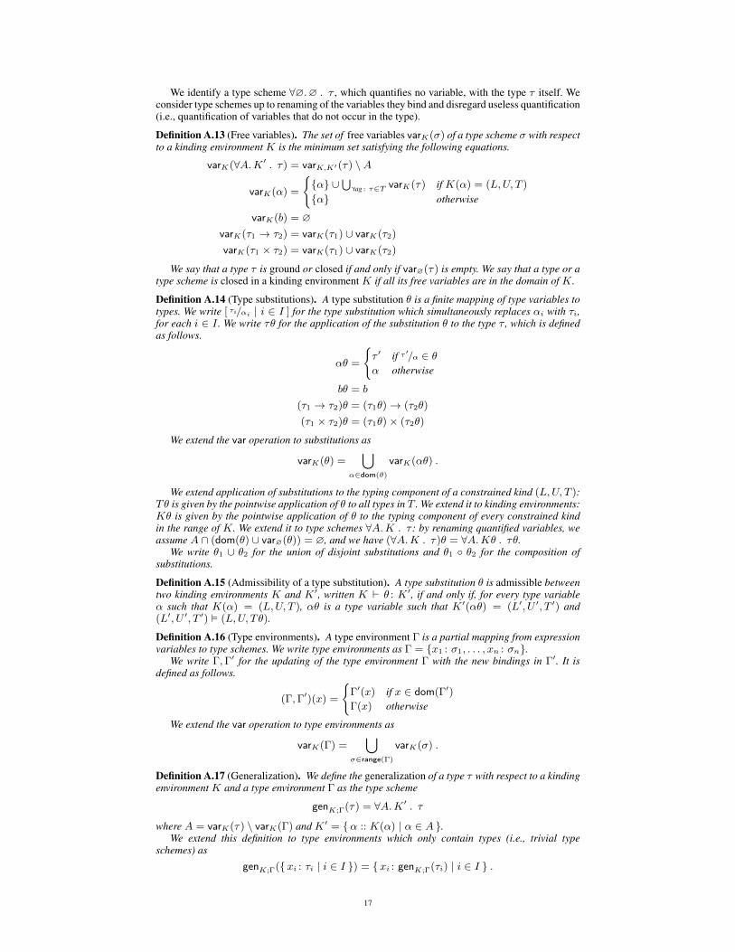
We identify a type scheme ∀∅.∅ . τ , which quantifies no variable, with the type τ itself. Weconsider type schemes up to renaming of the variables they bind and disregard useless quantification(i.e., quantification of variables that do not occur in the type).

Definition A.13 (Free variables). The set of free variables varK(σ) of a type scheme σ with respectto a kinding environment K is the minimum set satisfying the following equations.

varK(∀A.K′ . τ) = varK,K′(τ) \A

varK(α) =

α ∪

⋃tag : τ∈T varK(τ) if K(α) = (L,U, T )

α otherwise

varK(b) = ∅varK(τ1 → τ2) = varK(τ1) ∪ varK(τ2)

varK(τ1 × τ2) = varK(τ1) ∪ varK(τ2)

We say that a type τ is ground or closed if and only if var∅(τ) is empty. We say that a type or atype scheme is closed in a kinding environment K if all its free variables are in the domain of K.

Definition A.14 (Type substitutions). A type substitution θ is a finite mapping of type variables totypes. We write [ τi/αi | i ∈ I ] for the type substitution which simultaneously replaces αi with τi,for each i ∈ I . We write τθ for the application of the substitution θ to the type τ , which is definedas follows.

αθ =

τ ′ if τ ′/α ∈ θα otherwise

bθ = b

(τ1 → τ2)θ = (τ1θ)→ (τ2θ)

(τ1 × τ2)θ = (τ1θ)× (τ2θ)

We extend the var operation to substitutions as

varK(θ) =⋃

α∈dom(θ)

varK(αθ) .

We extend application of substitutions to the typing component of a constrained kind (L,U, T ):Tθ is given by the pointwise application of θ to all types in T . We extend it to kinding environments:Kθ is given by the pointwise application of θ to the typing component of every constrained kindin the range of K. We extend it to type schemes ∀A.K . τ : by renaming quantified variables, weassume A ∩ (dom(θ) ∪ var∅(θ)) = ∅, and we have (∀A.K . τ)θ = ∀A.Kθ . τθ.

We write θ1 ∪ θ2 for the union of disjoint substitutions and θ1 θ2 for the composition ofsubstitutions.

Definition A.15 (Admissibility of a type substitution). A type substitution θ is admissible betweentwo kinding environments K and K′, written K ` θ : K′, if and only if, for every type variableα such that K(α) = (L,U, T ), αθ is a type variable such that K′(αθ) = (L′, U ′, T ′) and(L′, U ′, T ′) (L,U, Tθ).

Definition A.16 (Type environments). A type environment Γ is a partial mapping from expressionvariables to type schemes. We write type environments as Γ = x1 : σ1, . . . , xn : σn.

We write Γ,Γ′ for the updating of the type environment Γ with the new bindings in Γ′. It isdefined as follows.

(Γ,Γ′)(x) =

Γ′(x) if x ∈ dom(Γ′)

Γ(x) otherwise

We extend the var operation to type environments as

varK(Γ) =⋃

σ∈range(Γ)

varK(σ) .

Definition A.17 (Generalization). We define the generalization of a type τ with respect to a kindingenvironment K and a type environment Γ as the type scheme

genK;Γ(τ) = ∀A.K′ . τ

where A = varK(τ) \ varK(Γ) and K′ = α :: K(α) | α ∈ A .We extend this definition to type environments which only contain types (i.e., trivial type

schemes) as

genK;Γ(xi : τi | i ∈ I ) = xi : genK;Γ(τi) | i ∈ I .

17

TPk-WildcardK ` : τ ⇒ ∅

TPk-VarK ` x : τ ⇒ x : τ

TPk-ConstK ` c : bc ⇒ ∅

TPk-PairK ` p1 : τ1 ⇒ Γ1 K ` p2 : τ2 ⇒ Γ2

K ` (p1, p2) : τ1 × τ2 ⇒ Γ1 ∪ Γ2

TPk-TagK ` p : τ ⇒ Γ K(α) = (L,U, T ) ( tag ∈ U implies tag : τ ∈ T )

K ` tag(p) : α⇒ Γ

TPk-AndK ` p1 : τ ⇒ Γ1 K ` p2 : τ ⇒ Γ2

K ` p1&p2 : τ ⇒ Γ1 ∪ Γ2

TPk-OrK ` p1 : τ ⇒ Γ K ` p2 : τ ⇒ Γ

K ` p1|p2 : τ ⇒ Γ

Figure 8. Pattern environment generation for K.

Tk-Varτ ∈ instK(Γ(x))

K; ΓKx : τ

Tk-ConstK; Γ

Kc : bc

Tk-AbstrK; Γ, x : τ1 K

e : τ2

K; ΓKλx. e : τ1 → τ2

Tk-ApplK; Γ

Ke1 : τ ′ → τ K; Γ

Ke2 : τ ′

K; ΓKe1 e2 : τ

Tk-PairK; Γ

Ke1 : τ1 K; Γ

Ke2 : τ2

K; ΓK

(e1, e2) : τ1 × τ2

Tk-TagK; Γ

Ke : τ K(α) ( tag,L, tag : τ)

K; ΓK

tag(e) : α

Tk-Match

K; ΓKe0 : τ0 τ0 4K pi | i ∈ I

∀i ∈ I K ` pi : τ0 ⇒ Γi K; Γ, genK;Γ(Γi) Kei : τ

K; ΓKmatch e0 with (pi → ei)i∈I : τ

Figure 9. Typing relation for K.

Definition A.18 (Instances of a type scheme). The set of instances of a type scheme ∀A.K′ . τ ina kinding environment K is defined as

instK(∀A.K′ . τ) = τθ | dom(θ) ⊆ A ∧ K,K′ ` θ : K .We say that a type scheme σ1 is more general than a type scheme σ2 in K, and we write

σ1 vK σ2, if instK(σ1) ⊇ instK(σ2).We extend this notion to type environments as

Γ1 vK Γ2 ⇐⇒ dom(Γ1) = dom(Γ2) ∧ ∀x ∈ dom(Γ1). Γ1(x) vK Γ2(x) .

Definition A.19 (Pattern environment generation). The environment generated by pattern matchingis given by the relationK ` p : τ ⇒ Γ (the pattern p can match type τ inK, producing the bindingsin Γ), defined by the rules in Figure 8.

Definition A.20 (Exhaustiveness). We say that a set of patterns P is exhaustive with respect to atype τ in a kinding environment K, and we write τ 4K P , when

∀K′, θ, v. (K ` θ : K′ ∧ K′;∅Kv : τθ) =⇒ ∃p ∈ P, ς. v/p = ς .

Definition A.21 (Typing relation). The typing relation K; ΓKe : τ (e is given type τ in the

kinding environment K and the type environment Γ) is defined by the rules in Figure 9, where werequire K to be closed and Γ and τ to be closed with respect to K. We also assume that K iscanonical.

A.2.2 Properties of the K type systemLemma A.1 (Generation for values). Let v be a value. Then:

• if K; ΓKv : b, then v = c for some constant c such that bc = b;

• if K; ΓKv : τ1 → τ2, then v is of the form λx. e and K; Γ, x : τ1 K

e : τ2;• if K; Γ

Kv : τ1 × τ2, then v is of the form (v1, v2), K; Γ

Kv1 : τ1, and K; Γ

Kv2 : τ2;

18

• if K; ΓKv : α, then v is of the form tag(v1), K(α) = (L,U, T ), tag ∈ L, and

K; ΓKv1 : τ1 for the only type τ1 such that tag : τ1 ∈ T .

Proof. The typing rules are syntax-directed, so the last rule applied to type a value is fixed byits form. All these rules derive types of different forms, thus the form of the type assigned to avalue determines the last rule used. In each case the premises of the rule entail the consequencesabove.

Lemma A.2 (Correctness of environment generation). Let p be a pattern and v a value such thatv/p = ς . If K; Γ

Kv : τ and K ` p : τ ⇒ Γ′, then, for all x ∈ capt(p), K; Γ

Kxς : Γ′(x).

Proof. By induction on the derivation of K ` p : τ ⇒ Γ′. We reason by cases on the last appliedrule.

Cases TPk-Wildcard and TPk-Const There is nothing to prove since capt(p) = ∅.

Case TPk-Var We havev/x = [v/x] K ` x : τ ⇒ x : τ

and must prove K; ΓKx[v/x] : x : τ(x), which we know by hypothesis.

Case TPk-Pair We have

K ` (p1, p2) : τ1 × τ2 ⇒ Γ′1 ∪ Γ′2 K ` p1 : τ1 ⇒ Γ′1 K ` p2 : τ2 ⇒ Γ′2 .

By Lemma A.1, K; ΓKv : τ1 × τ2 implies v = (v1, v2) and K; Γ

Kvi : τi for both i.

Furthermore, (v1, v2)/(p1, p2) = ς = ς1 ∪ ς2, and vi/pi = ςi for both i. For each capturevariable x, we can apply the induction hypothesis to the sub-pattern which contains x andconclude.

Case TPk-Tag We have

K ` tag(p1) : α⇒ Γ′ K ` p1 : τ1 ⇒ Γ′

K(α) = (L,U, T ) ( tag ∈ U implies tag : τ1 ∈ T ) .

Since v/ tag(p1) = ς , we know v = tag(v1). Hence, by Lemma A.1, we have tag ∈ Land K; Γ

Kv1 : τ ′1 with tag : τ ′1 ∈ T . Since tag ∈ U , we also have tag : τ1 ∈ T and hence

τ1 = τ ′1 (as tag is also in L and can only have a single type in T ).We therefore know K ` p1 : τ1 ⇒ Γ′ and K; Γ

Kv1 : τ1, as well as v1/p1 = ς . We can

apply the induction hypothesis to conclude.

Cases TPk-And and TPk-Or Straightforward application of the induction hypothesis, to bothsub-patterns for intersections and to the one that is actually selected for unions.

Lemma A.3 (Stability of environment generation under type substitutions). If K ` p : τ ⇒ Γ,then K′ ` p : τθ ⇒ Γθ for every type substitution θ such that K ` θ : K′.

Proof. By induction on the derivation of K ` p : τ ⇒ Γ. We reason by cases on the last appliedrule.

Cases TPk-Wildcard, TPk-Var, and TPk-Const Straightforward.

Case TPk-Pair We have

K ` (p1, p2) : τ1 × τ2 ⇒ Γ1 ∪ Γ2 K ` p1 : τ1 ⇒ Γ1 K ` p2 : τ2 ⇒ Γ2 .

By the induction hypothesis we derive both K′ ` p1 : τ1θ ⇒ Γ1θ and K′ ` p2 : τ2θ ⇒Γ2θ, then we apply TPk-Pair again to conclude.

Case TPk-Tag We have

K ` tag(p1) : α⇒ Γ K ` p1 : τ1 ⇒ Γ

K(α) = (L,U, T ) ( tag ∈ U implies tag : τ1 ∈ T ) .

By the induction hypothesis we derive K′ ` p1 : τ1θ ⇒ Γθ. Since K ` θ : K′, αθmust be a variable β such that K′(β) = (L′, U ′, T ′). To apply TPk-Tag and conclude, wemust establish that, if tag ∈ U ′, then tag : τ1θ ∈ T ′. Since admissibility also implies(L′, U ′, T ′) (L,U, Tθ), we have U ′ ⊆ U and Tθ ⊆ T ′. Hence, if tag ∈ U ′, then tag ∈ U ,in which case tag : τ1 ∈ T and therefore tag : τ1θ ∈ Tθ, and tag : τ1θ ∈ T ′.

Cases TPk-And and TPk-Or Straightforward application of the induction hypothesis, analogouslyto the case of pair patterns.

19

Lemma A.4 (Stability of exhaustiveness under type substitutions). If τ 4K P , then τθ 4K′ P forany type substitution θ such that K ` θ : K′.

Proof. We must prove, for every K′′, θ′ such that K′ ` θ′ : K′′ and every v such that K′′;∅K

v : τθθ′, that there exists a p ∈ P which accepts v. This holds because θ′ θ is such thatK ` θ′ θ : K′′: for any α such that K(α) = (L,U, T ), we have K′(αθ) = (L′, U ′, T ′)and hence K′′(αθθ′) = (L′′, U ′′, T ′′); we have (L′, U ′, T ′) (L,U, Tθ) and (L′′, U ′′, T ′′) (L′, U ′, T ′θ′) and therefore (L′′, U ′′, T ′′) (L,U, Tθθ′). The conclusion follows by the defini-tion of τ 4K P .

Lemma A.5. If varK(Γ1) ⊆ varK(Γ2), then, for every type τ , genK;Γ1(τ) vK genK;Γ2

(τ).

Proof. An instance of genK;Γ2(τ) is a type τθ such that dom(θ) ⊆ varK(τ) \ varK(Γ2) and

K ` θ : K. It is also an instance of genK;Γ1(τ), with the same θ, since varK(τ) \ varK(Γ2) ⊆

varK(τ) \ varK(Γ1).

Lemma A.6 (Weakening). LetK be a kinding environment and Γ1, Γ2 two type environments suchthat Γ1 vK Γ2 and varK(Γ1) ⊆ varK(Γ2). If K; Γ2 K

e : τ , then K; Γ1 Ke : τ .

Proof. By induction on the derivation ofK; Γ2 Ke : τ . We reason by cases on the last applied rule.

Case Tk-Var We have:K; Γ2 K

x : τ τ ∈ instK(Γ2(x))

and hence, since Γ1 vK Γ2, we have τ ∈ instK(Γ1(x)) and apply Tk-Var to conclude.

Case Tk-Const Straightforward.

Case Tk-Abstr We have:

K; Γ2 Kλx. e1 : τ1 → τ2 K; Γ2, x : τ1 K

e1 : τ2 .

Since Γ1 vK Γ2, we have Γ1, x : τ1 vK Γ2, x : τ1, and, since varK(Γ1) ⊆ varK(Γ2),we have varK(Γ1, x : τ1) ⊆ varK(Γ2, x : τ1). Thus we may derive K; Γ1, x : τ1 K

e1 : τ2 by the induction hypothesis and apply Tk-Abstr to conclude.

Cases Tk-Appl, Tk-Pair, and Tk-Tag Straightforward application of the induction hypothesis.

Case Tk-Match We have

K; Γ2 Kmatch e0 with (pi → ei)i∈I : τ

K; Γ2 Ke0 : τ0 τ0 4K pi | i ∈ I

∀i ∈ I. K ` pi : τ0 ⇒ Γi K; Γ2, genK;Γ2(Γi) K

ei : τ .

By the induction hypothesis, we derive K; Γ1 Ke0 : τ0.

For every branch, note that by Lemma A.5 varK(Γ1) ⊆ varK(Γ2) implies genK;Γ1(τ) vK

genK;Γ2(τ) for any τ . Hence, we have Γ1, genK;Γ1

(Γi) vK Γ2, genK;Γ2(Γi). Additionally,

since varK(genK;Γ1(Γi)) ⊆ varK(Γ1), we have varK(Γ1, genK;Γ1

(Γi)) ⊆ varK(Γ2, genK;Γ2(Γi)).

Hence we may apply the induction hypothesis for all i to derive K; Γ1, genK;Γ1(Γi) K

ei : τ and then apply Tk-Match to conclude.

Lemma A.7 (Stability of typing under type substitutions). Let K, K′ be two closed, canonicalkinding environments and θ a type substitution such that K ` θ : K′. If K; Γ

Ke : τ , then

K′; ΓθKe : τθ.

Proof. By induction on the derivation of K; ΓKe : τ . We reason by cases on the last applied rule.

Case Tk-Var We have

K; ΓKx : τ τ ∈ instK(Γ(x))

Γ(x) = ∀A.Kx . τx τ = τxθx dom(θx) ⊆ A K,Kx ` θx : K

and must showK′; Γθ

Kx : τθ .

By α-renaming we can assume that θ does not involve A, that is, A ∩ dom(θ) = ∅ andA∩ var∅(θ) = ∅, and also that A∩ (dom(K′)∪ var∅(K′)) = ∅, that is, that the variables inA are not assigned a kind in K′ nor do they appear in the types in the typing component of thekinds in K′.

Under these assumptions, (Γθ)(x) = ∀A.Kxθ . τxθ. We must show that τθ = τxθθ′x for a

substitution θ′x such that dom(θ′x) ⊆ A and K′,Kxθ ` θ′x : K′.

20

Let θ′x = [ αθxθ/α | α ∈ A ]. First, we show that τxθθ′x = τxθxθ = τθ, by showing that, forany α, αθθ′x = αθxθ. If α ∈ A, then αθθ′x = αθ′x = αθxθ (θ is not defined on the variablesin A). If α /∈ A, then αθθ′x = αθ (θ never produces any variable in A) and αθxθ = αθ asα /∈ dom(θx).

Since dom(θ′x) ⊆ A holds, we only need to establish thatK′,Kxθ ` θ′x : K′. This requiresproving, for each α such that (K′,Kxθ)(α) = (L,U, T ), that αθ′x is a type variable such thatK′(αθ′x) = (L′, U ′, T ′) and (L′, U ′, T ′) (L,U, Tθ′x).

Such an α can either be in the domain of Kxθ (if and only if it is in A) or in the domain ofK′. In the latter case, we have αθ′x = α, since α /∈ A, and hence its kind in K′ is the same asin K′,Kxθ. We must prove (L,U, T ) (L,U, Tθ′x), which holds because the variables in Ado not appear in T since (L,U, T ) ∈ range(K′).

In the former case, we have (Kxθ)(α) = (L,U, T ) and hence Kx(α) = (L,U, T1), withT = T1θ. Also, αθ′x = αθxθ. Since K,Kx ` θx : K, K(αθx) = (L2, U2, T2). Then,since K ` θ : K′, K′(αθxθ) = (L′, U ′, T ′). We know (L2, U2, T2) (L,U, T1θx) and(L′, U ′, T ′) (L2, U2, T2θ). Both L′ ⊇ L and U ′ ⊆ U hold by transitivity. We showT ′ ⊇ Tθ′x holds as well. If tag : τ ∈ Tθ′x, since T = T1θ, then tag : τ1 ∈ T1 andτ = τ1θθ

′x = τ1θxθ. We thus have tag : τ1θx ∈ T1θx and therefore tag : τ1θx ∈ T2 and

tag : τ1θxθ ∈ T ′.

Case Tk-Const Straightforward.

Case Tk-Abstr We have:

K; ΓKλx. e1 : τ1 → τ2 K; Γ, x : τ1 K

e1 : τ2 .

By the induction hypothesis we have K′; Γθ, x : τ1θ Ke1 : τ2θ. Then by Tk-Abstr we

derive K′; ΓθKλx. e1 : (τ1 → τ2)θ, since (τ1 → τ2)θ = (τ1θ)→ (τ2θ).

Cases Tk-Appl and Tk-Pair Straightforward application of the induction hypothesis.

Case Tk-Match For the sake of clarity, we first prove the simpler case corresponding to (theencoding of) let, where—simplifying environment generation—we have

K; ΓKmatch e0 with x→ e1 : τ K; Γ

Ke0 : τ0 K; Γ, genK;Γ(x : τ0) K

e1 : τ

and must showK′; Γθ

Kmatch e0 with x→ e1 : τθ

which we prove by establishing, for some type τ0, that

K′; ΓθKe0 : τ0 K′; Γθ, genK′;Γθ(x : τ0) K

e1 : τθ .

Let A = α1, . . . , αn = varK(τ0) \ varK(Γ). We assume that the variables in A do notappear in the kinds of variables not in A, that is, that if K(α) = (L,U, T ) and α /∈ A, thenvarK(T ) ∩A = ∅.

This assumption is justified by the following observations. The variables in A only appearquantified in the environment used for the typing derivation for e1. Therefore we may assumethat they do not appear in τ : if they do, it is because they have been chosen when instantiatingsome type scheme and, since K is canonical, we might have chosen some other variable ofthe same kind. As for the occurrences of the variables in A in the derivation for e0, a similarreasoning applies. These variables do not appear free in the environment (neither directly in atype in Γ, nor in the kinds of variables which appear free in Γ). Therefore, if they occur in τ0it is because they have been chosen either during instantiation of a type scheme or when typingan abstraction, and in both cases we might have chosen a different variable.

Now we rename these variables so that θ will not have effect on them. Let B =β1, . . . , βn be a set of type variables such that B ∩ (dom(θ) ∪ var∅(θ)) = ∅ andB ∩ var∅(Γ) = ∅. Let θ0 = [β1/α1, . . . , βn/αn] and θ′ = θ θ0. Since K′ is canonical,we can choose each βi so that, if K(αi) = •, then K′(βi) = •, and if K(αi) = (L,U, T ),then K(βi) = (L,U, Tθ′). As for A, we choose B so that the kinds in K′ for variables not inB do not contain variables of B.

We show K ` θ′ : K′. For each α such that K(α) = (L,U, T ), if α ∈ A then α = αifor some i, αθ′ = βi and kind entailment holds straightforwardly by our choice of βi. Ifα /∈ A, then αθ′ = αθ and the admissibility of θ implies K′(αθ) = (L′, U ′, T ′) and(L′, U ′, T ′) (L,U, Tθ). We have Tθ = Tθ′ because of our assumption on A.

Since θ′ is admissibile, by the induction hypothesis applied to θ′, we derive K; Γθ′K

e0 : τ0θ′. Since the variables in A do not appear in Γ, we have Γθ′ = Γθ. We choose τ0 to be

τ0θ′.We apply the induction hypothesis to the derivation for e1, this time using θ as the substitu-

tion. Now we have:

K′; ΓθKe0 : τ0θ

′ K′; Γθ, (genK;Γ(x : τ0))θ Ke1 : τθ .

21

We apply weakening (Lemma A.6) to derive from the latter the typing we need, that is,

K′; Γθ, genK′;Γθ(x : τ0θ′)

Ke1 : τθ .

To do so we must show

Γθ, genK′;Γθ(x : τ0θ′) vK′ Γθ, (genK;Γ(x : τ0))θ

varK′(Γθ, genK′;Γθ(x : τ0θ′)) ⊆ varK′(Γθ, (genK;Γ(x : τ0))θ) .

The latter holds because varK′(Γθ, genK′;Γθ(x : τ0θ′)) ⊆ varK′(Γθ).

As for the former, we prove genK′;Γθ(x : τ0θ′) vK′ (genK;Γ(x : τ0))θ. We have

genK;Γ(x : τ0) = ∀A.Kx . τ0 Kx = α :: K(α) | α ∈ A .By α-renaming of the quantified variables we can write

genK;Γ(x : τ0) = ∀B.K?x . τ0θ0

K?x = βi :: • | αi :: • ∈ Kx ∪ βi :: (L,U, Tθ0) | αi :: (L,U, T ) ∈ A

and, since θ does not involve B,

(genK;Γ(x : τ0))θ = ∀B.K?xθ . τ0θ0θ = ∀B.K′x . τ0θ′

K′x = β :: K′(β) | β ∈ B .The other type scheme is

genK′;Γθ(τ0θ′) = ∀C.K′C . τ0θ′

C = varK′(τ0θ′) \ varK′(Γθ) K′C = β :: K′(β) | β ∈ C .

We show B ⊆ C, which concludes the proof (because the kinding environments areboth restrictions of K′). Consider βi ∈ B. We have αi ∈ varK(τ0) \ varK(Γ). Thenβi = αiθ

′ ∈ varK′(τ0θ′). Furthermore βi /∈ varK′(Γθ) holds because Γθ does not contain

variables in B (Γ does not contain them and θ does not introduce them) and variables in B donot appear in the kinds of other variables which are not themselves in B.

We now consider the rule Tk-Match in its generality. We have

K; ΓKmatch e0 with (pi → ei)i∈I : τ

K; ΓKe0 : τ0 τ0 4K pi | i ∈ I

∀i ∈ I. K ` pi : τ0 ⇒ Γi K; Γ, genK;Γ(Γi) Kei : τ

and must show

K′; ΓθKmatch e0 with (pi → ei)i∈I : τθ

which we prove by establishing, for some τ0 and Γi | i ∈ I , that

K′; ΓθKe0 : τ0 τ0 4K′ pi | i ∈ I

∀i ∈ I. K′ ` pi : τ0 ⇒ Γi K′; Γθ, genK′;Γθ(Γi) Kei : τθ .

For the derivation for e0 we proceed as above and have τ0 = τ0θ′. By Lemma A.4 we have

τ0θ′ 4K′ pi | i ∈ I . By Lemma A.3, we have K′ ` pi : τ0θ

′ ⇒ Γiθ′ and thus take

Γi = Γiθ′.

We proceed as before also for the derivations for each branch. The difference is that, toapply weakening, we must prove the two premises for the environments and not for τ0 alone.The condition on variables is straightforward, as before. For the other we prove, for eachx ∈ capt(pi) and assuming Γi(x) = τx,

Γθ, genK′;Γθ(τxθ′) vK′ Γθ, (genK;Γ(τx))θ .

We show it as for τ0 above: varK(τx) is always a subset of varK(τ0) because environmentgeneration does not introduce new variables.

Lemma A.8 (Expression substitution). Let x1, . . . , xn be distinct variables and v1, . . . , vn values.Let Γ′ = x1 : σ1, . . . , xn : σn and ς = [v1/x1, . . . , vn/xn].

If K; Γ,Γ′Ke : τ and, for all k ∈ 1, . . . , n and for all τk ∈ instK(σk), K; Γ

Kvk : τk,

then K; ΓKeς : τ .

Proof. By induction on the derivation of K; Γ,Γ′Ke : τ . We reason by cases on the last applied

rule.

Case Tk-Var We have

K; Γ,Γ′Kx : τ τ ∈ instK((Γ,Γ′)(x)) .

22

Either x = xk for some k or not. In the latter case, xς = x, x /∈ dom(Γ′) and hence(Γ,Γ′)(x) = Γ(x). Then, since τ ∈ instK((Γ,Γ′)(x)), τ ∈ instK(Γ(x)) and Tk-Var can beapplied.

If x = xk, then (Γ,Γ′)(x) = Γ′(x) = σk. We must then prove K; ΓKvk : τ , which we

know by hypothesis since τ ∈ instK(σk).

Case Tk-Const Straightforward.

Case Tk-Abstr We have

K; Γ,Γ′Kλx. e1 : τ1 → τ2 K; Γ,Γ′, x : τ1 K

e1 : τ2 .

Byα-renaming we can assume x /∈ dom(Γ′); then (λx. e1)ς = λx. (e1ς) and Γ,Γ′, x : τ1 =Γ, x : τ1,Γ′. Therefore we have K; Γ, x : τ1,Γ′ K

e1 : τ2 and, by the induction hypothe-sis, K; Γ, x : τ1 K

e1ς : τ2. We apply Tk-Abstr to conclude.

Cases Tk-Appl, Tk-Pair, and Tk-Tag Straightforward application of the induction hypothesis.

Case Tk-Match We have

K; Γ,Γ′Kmatch e0 with (pi → ei)i∈I : τ

K; Γ,Γ′Ke0 : τ0 τ0 4K pi | i ∈ I

∀i ∈ I. K ` pi : τ0 ⇒ Γi K; Γ,Γ′, genK;Γ,Γ′(Γi) Kei : τ .

We assume by α-renaming that no capture variable of any pattern is in the domainof Γ′. Then, (match e0 with (pi → ei)i∈I)ς = match e0ς with (pi → eiς)i∈I andΓ,Γ′, genK;Γ,Γ′(Γi) = Γ, genK;Γ,Γ′(Γi),Γ

′ for any i.By the induction hypothesis, we derive K; Γ

Ke0ς : τ0 and K; Γ, genK;Γ,Γ′(Γi) K

eiς : τfor all i. From the latter, we prove K; Γ, genK;Γ(Γi) K

eiς : τ by weakening (Lemma A.6):we have genK;Γ(Γi) vK genK;Γ,Γ′(Γi) by Lemma A.5—since varK(Γ) ⊆ varK(Γ,Γ′)—andclearly we have varK(Γ, genK;Γ(Γi)) ⊆ varK(Γ, genK;Γ,Γ′(Γi)) since varK(genK;Γ(Γi)) ⊆varK(Γ).

Theorem A.9 (Progress). Let e be a well-typed, closed expression. Then, either e is a value orthere exists an expression e′ such that e e′.

Proof. By hypothesis we have K;∅Ke : τ . The proof is by induction on its derivation; we reason

by cases on the last applied rule.

Case Tk-Var This case does not occur because variables are not closed.

Case Tk-Const In this case e is a constant c and therefore a value.

Case Tk-Abstr In this case e is an abstraction λx. e1. Since it is also closed, it is a value.

Case Tk-Appl We have

K;∅Ke1 e2 : τ K;∅

Ke1 : τ ′ → τ K;∅

Ke2 : τ ′ .

By the induction hypothesis, each of e1 and e2 either is a value or may reduce. If e1 e′1,then e1 e2 e′1 e2. If e1 is a value and e2 e′2, then e1 e2 e1 e

′2.

If both are values then, by Lemma A.1, e1 has the form λx. e3 for some e3. Then, we canapply R-Appl and e1 e2 e3[e2/x].

Case Tk-Pair We have

K;∅K

(e1, e2) : τ1 × τ2 K;∅Ke1 : τ1 K;∅

Ke2 : τ2 .

By the induction hypothesis, each of e1 and e2 either is a value or may reduce. If e1 e′1,then (e1, e2) (e′1, e2). If e1 is a value and e2 e′2, then (e1, e2) (e1, e

′2). If both are

values, then (e1, e2) is also a value.

Case Tk-Tag We haveK;∅

Ktag(e1) : α K;∅

Ke1 : τ1 .

Analogously to the previous case, by the induction hypothesis we have that either e1 isa value or e1 e′1. In the former case, tag(e1) is a value as well. In the latter, we havetag(e1) tag(e′1).

Case Tk-Match We have

K;∅Kmatch e0 with (pi → ei)i∈I : τ K;∅

Ke0 : τ0 τ0 4K pi | i ∈ I .

By the inductive hypothesis, either e0 is a value or it may reduce. In the latter case, ife0 e′0, then match e0 with (pi → ei)i∈I match e′0 with (pi → ei)i∈I .

23

If e0 is a value, on the other hand, the expression may reduce by application of R-Match.Since τ0 4K pi | i ∈ I and e0 is a value of type τ0 (and therefore satisfies the premises ofthe definition of exhaustiveness, with θ = [ ] and K = K′), there exists at least an i ∈ I suchthat e0/pi = ς for some substitution ς . Let j be the least of these i and ςj the correspondingsubstitution; then match e0 with (pi → ei)i∈I ejςj .

Theorem A.10 (Subject reduction). Let e be an expression and τ a type such that K; ΓKe : τ . If

e e′, then K; ΓKe′ : τ .

Proof. By induction on the derivation of K; ΓKe : τ . We reason by cases on the last applied rule.

Cases Tk-Var, Tk-Const, and Tk-Abstr These cases may not occur: variables, constants, andabstractions never reduce.

Case Tk-Appl We have

K; ΓKe1 e2 : τ K; Γ

Ke1 : τ ′ → τ K; Γ

Ke2 : τ ′ .

e1 e2 e′ occurs in any of three ways: (i) e1 e′1 and e′ = e′1 e2; (ii) e1 is a value,e2 e′2 and e′ = e1 e

′2; (iii) both e1 and e2 are values, e1 is of the form λx. e3, and

e′ = e3[e2/x].In the first case, we derive by the induction hypothesis thatK; Γ

Ke′1 : τ ′ → τ and conclude

by applying Tk-Appl again. The second case is analogous.In the third case, we know by Lemma A.1 that K; Γ, x : τ ′

Ke3 : τ . We also know that

e2 is a value such that K; ΓKe2 : τ ′. Then, by Lemma A.8, K; Γ

Ke3[e2/x] : τ .

Case Tk-Pair We have

K; ΓK

(e1, e2) : τ1 × τ2 K; ΓKe1 : τ1 K; Γ

Ke2 : τ2 .

(e1, e2) e′ occurs either because e1 e′1 and e′ = (e′1, e2), or because e1 is a value,e2 e′2, and e′ = (e1, e

′2). In either case, the induction hypothesis allows us to derive that

the type of the component that reduces is preserved; therefore, we can apply Tk-Pair again toconclude.

Case Tk-Tag Analogously to the previous case, a variant expression only reduces if its argumentdoes, so we apply the induction hypothesis and Tk-Tag to conclude.

Case Tk-Match We have

K; ΓKmatch e0 with (pi → ei)i∈I : τ

K; ΓKe0 : τ0 ∀i ∈ I. K ` pi : τ0 ⇒ Γi K; Γ, genK;Γ(Γi) K

ei : τ .

match e0 with (pi → ei)i∈I e′ occurs either because e0 e′0 and e′ = match e′0 with(pi → ei)i∈I or because e0 is a value and e′ = ejς , where e0/pj = ς and, for all i < j,e0/pi = Ω. In the former case, we apply the induction hypothesis and conclude by Tk-Match.

In the latter case, ς is a substitution from the capture variables of pj to values, and we knowby Lemma A.2 that, for all x ∈ capt(pj), K; Γ

Kxς : Γj(x). We show that, additionally,

K; ΓKxς : τx holds for every τx ∈ instK(genK;Γ(Γj(x))). Every such τx is equal to

Γj(x)θ for a θ such that dom(θ) ⊆ varK(Γj(x)) \ varK(Γ) and K ` θ : K (the kindingenvironment captured by generalization is just a subset of K). Then, K; Γ

Kxς : Γj(x)θ holds

by Lemma A.14, since Γθ = Γ (the substitution does not change any free variable of Γ).From K; Γ, genK;Γ(Γj) K

ej : τ and from the fact that we have K; ΓKxς : τx for

all x ∈ dom(Γj) and all τx ∈ instK(genK;Γ(Γj(x))), we derive K; ΓKejς : τ by

Lemma A.8.

Corollary A.11 (Type soundness). Let e be a well-typed, closed expression, that is, such thatK;∅

Ke : τ holds for some τ . Then, either e diverges or it reduces to a value v such that

K;∅Kv : τ .

Proof. Consequence of Theorem A.9 and Theorem A.10.

A.3 Typing variants with set-theoretic typesA.3.1 Definition of the S type systemWe consider a set V of type variables (ranged over by α, β, γ, . . . ) and the sets C, L, and B oflanguage constants, tags, and basic types (ranged over by c, tag, and b respectively).

Definition A.22 (Types). A type t is a term coinductively produced by the following grammar:

t ::= α | b | c | t→ t | t× t | tag(t) | t ∨ t | ¬t | 0which satisfies two additional constraints:

24

• (regularity) the term must have a finite number of different sub-terms;• (contractivity) every infinite branch must contain an infinite number of occurrences of atoms

(i.e., a type variable or the immediate application of a type constructor: basic, constant, arrow,product, or variant).

We introduce the following abbreviations:

t1 ∧ t2def= ¬(¬t1 ∨ ¬t2) t1 \ t2

def= t1 ∧ (¬t2) 1

def= ¬0 .

Definition A.23 (Type schemes). A type scheme s is of the form ∀A. t, where A is a finite setα1, . . . , αn of type variables.

We identify a type scheme ∀∅. t with the type t itself. Furthermore, we consider type schemesup to renaming of the variables they bind, and we disregard useless quantification.

Definition A.24 (Free variables). We write var(t) for the set of type variables occurring in a typet; we say they are the free variables of t, and we say that t is ground or closed if and only if var(t)is empty.

We extend the definition to type schemes as var(∀A. t) = var(t) \A.

The (coinductive) definition of var can be found in Castagna et al. (2014, Definition A.2).

Definition A.25 (Meaningful variables). We define the set mvar(t) of meaningful variables of atype t as

mvar(t) = α ∈ var(t) | t[0/α] 6' t .We extend the definition to type schemes as mvar(∀A. t) = mvar(t) \A.

Definition A.26 (Type substitutions). A type substitution θ is a finite mapping of type variables totypes. We write [ ti/αi | i ∈ I ] for the type substitution which simultaneously replaces αi with ti,for each i ∈ I . We write tθ for the application of the substitution θ to the type t; application isdefined coinductively by the following equations.

αθ =

t′ if t′/α ∈ θα otherwise

bθ = b

cθ = c

(t1 → t2)θ = (t1θ)→ (t2θ)

(t1 × t2)θ = (t1θ)× (t2θ)

( tag(t))θ = tag(tθ)

(t1 ∨ t2)θ = (t1θ) ∨ (t2θ)

(¬t)θ = ¬(tθ)

0θ = 0

We extend the var operation to substitutions as

var(θ) =⋃

α∈dom(θ)

var(αθ) .

and we extend mvar likewise.We extend application of substitutions to type schemes ∀A. t: by renaming quantified variables,

we assume A ∩ (dom(θ) ∪ var(θ)) = ∅, and we have (∀A. t)θ = ∀A. tθ.We write θ1 ∪ θ2 for the union of disjoint substitutions and θ1 θ2 for the composition of

substitutions.

Definition A.27 (Type environments). A type environment Γ is a partial mapping from expressionvariables to type schemes. We write type environments as Γ = x1 : s1, . . . , xn : sn.

We write Γ,Γ′ for the updating of the type environment Γ with the new bindings in Γ′. It isdefined as follows.

(Γ,Γ′)(x) =

Γ′(x) if x ∈ dom(Γ′)

Γ(x) otherwise

We extend the var operation to type environments as

var(Γ) =⋃

s∈range(Γ)

var(s) ,

and we extend mvar likewise.

25

Definition A.28 (Generalization). We define the generalization of a type t with respect to the typeenvironment Γ as the type scheme

genΓ(t) = ∀A. twhere A = var(t) \mvar(Γ).

We extend this definition to type environments which only contain types (i.e., trivial typeschemes) as

genΓ(xi : ti | i ∈ I ) = xi : genΓ(ti) | i ∈ I .Definition A.29 (Instances of a type scheme). The set of instances of a type scheme ∀A. t is definedas

inst(∀A. t) = tθ | dom(θ) ⊆ A .We say that a type scheme s1 is more general than a type scheme s2, and we write s1 v s2, if

∀t2 ∈ inst(s2). ∃t1 ∈ inst(s1). t1 ≤ t2 .We extend this notion to type environments as

Γ1 v Γ2 ⇐⇒ dom(Γ1) = dom(Γ2) ∧ ∀x ∈ dom(Γ1). Γ1(x) v Γ2(x) .

Definition A.30 (Accepted type). The accepted type *p+ of a pattern p is defined inductively as:

* + = *x+ = 1 *c+ = c

*(p1, p2)+ = *p1+× *p2+ * tag(p)+ = tag(*p+)

*p1&p2+ = *p1+ ∧ *p2+ *p1|p2+ = *p1+ ∨ *p2+ .

The projection operators π1 and π2 for product types are defined by Castagna et al. (2014,Appendix C.2.1). We do not repeat the definition, but we state below the properties we need in theproofs. The projection operators for variant types correspond to π2 if we encode variant types aspairs; we therefore rephrase the same properties for them.

Property A.31 (Projections of product types). There exist two functions π1 and π2 which, given atype t ≤ 1× 1, yield types π1(t) and π2(t) such that:

• t ≤ π1(t)× π2(t);• if t ≤ t1 × t2, then πi(t) ≤ ti;• if t ≤ t′ ≤ 1× 1, then πi(t) ≤ πi(t′);• for all type substitutions θ, πi(tθ) ≤ πi(t)θ.

Property A.32 (Projections of variant arguments). For every tag tag there exists a function π tag

which, given a type t ≤ tag(1), yields a type π tag(t) such that:

• t ≤ tag(π tag(t));• if t ≤ tag(t′), then π tag(t) ≤ t′;• if t ≤ t′ ≤ tag(1), then π tag(t) ≤ π tag(t

′);• for all type substitutions θ, π tag(tθ) ≤ π tag(t)θ.

Definition A.33 (Pattern environment generation). Given a pattern p and a type t ≤ *p+, the typeenvironment t//p generated by pattern matching is defined inductively as:

t// = ∅t//x = x : tt//c = ∅

t//(p1, p2) = π1(t)//p1 ∪ π2(t)//p2

t// tag(p) = π tag(t)//p

t//p1&p2 = t//p1 ∪ t//p2

t//p1|p2 = (t ∧ *p1+)//p1 ∨∨ (t \ *p1+)//p2 ,

where (Γ ∨∨ Γ′)(x) = Γ(x) ∨ Γ′(x).

Definition A.34 (Typing relation). The typing relation ΓSe : t (e is given type t in the type

environment Γ) is defined by the rules in Figure 10.

A.3.2 Properties of the S type systemLemma A.12 (Generation for values). Let v be a value. Then:

• if ΓSv : c, then v = c;

• if ΓSv : b, then v = c for some c such that bc ≤ b;

• if ΓSv : t1 → t2, then v is of the form λx. e and Γ, x : t1 S

e : t2;

26

Ts-Vart ∈ inst(Γ(x))

ΓSx : t

Ts-ConstΓ

Sc : c

Ts-AbstrΓ, x : t1 S

e : t2

ΓSλx. e : t1 → t2

Ts-ApplΓ

Se1 : t′ → t Γ

Se2 : t′

ΓSe1 e2 : t

Ts-PairΓ

Se1 : t1 Γ

Se2 : t2

ΓS

(e1, e2) : t1 × t2

Ts-TagΓ

Se : t

ΓS

tag(e) : tag(t)

Ts-Match

ΓSe0 : t0 t0 ≤

∨i∈I*pi+ ti = (t0 \

∨j<i*pj+) ∧ *pi+

∀i ∈ I Γ, genΓ(ti//pi) Sei : t

′i

ΓSmatch e0 with (pi → ei)i∈I :

∨i∈I t

′i

Ts-SubsumΓ

Se : t′ t′ ≤ tΓ

Se : t

Figure 10. Typing relation of the S type system.

• if ΓSv : t1 × t2, then v is of the form (v1, v2), Γ

Sv1 : t1, and Γ

Sv2 : t2;

• if ΓSv : tag(t1), then v is of the form tag(v1) and Γ

Sv1 : t1.

Proof. By induction on the typing derivation: values must be typed by an application of the rulecorresponding to their form to appropriate premises, possibly followed by applications of Ts-Subsum.

The base cases are straightforward. In the inductive step, we just apply the induction hypothesis;for abstractions, the result follows from the behaviour of subtyping on arrow types.

We state the next three lemmas without proof, as they rely on the model of types which we havenot discussed. Details can be found in Frisch et al. (2008) and Castagna and Xu (2011), as well asin Alain Frisch’s PhD thesis.9

Lemma A.13. For each i ∈ I , let pi be a pattern. If ΓSv :∨i∈I*pi+, then there exists an i ∈ I

such that ΓSv : *pi+.

Lemma A.14. Let t be a type. Let t′ be a type such that either t′ = *p+ or t′ = ¬*p+, for somepattern p. If Γ

Sv : t and Γ

Sv : t′, then Γ

Sv : t ∧ t′.

Lemma A.15. Let v be a well-typed value (i.e., ∅Sv : t holds for some t) and p a pattern. Then:

• ∅Sv : *p+ holds if and only if v/p = ς for some substitution ς;

• ∅Sv : ¬*p+ holds if and only if v/p = Ω.

Lemma A.16. Let p be a pattern and t, t′ two types. If t ≤ t′ ≤ *p+, then, for all x ∈ capt(p),(t//p)(x) ≤ (t′//p)(x).

Proof. By structural induction on p.

Cases p = and p = c There is nothing to prove since capt(p) = ∅.

Case p = x We must prove (t//x)(x) ≤ (t′//x)(x), that is, t ≤ t′, which we know byhypothesis.

Case p = (p1, p2) Each x ∈ capt(p) is either in capt(p1) or in capt(p2). Assume x ∈ capt(pi);then, (t//p)(x) = (πi(t)//pi)(x) and (t′//p)(x) = (πi(t

′)//pi)(x). Since t ≤ t′ impliesπi(t) ≤ πi(t′) by Property A.31, we can apply the induction hypothesis to conclude.

Case p = tag(p) Analogous to the previous case, because t ≤ t′ implies π tag(t) ≤ π tag(t′) by

Property A.32.

Case p = p1&p2 Each x ∈ capt(p) is either in capt(p1) or in capt(p2). Assume x ∈ capt(pi);then, (t//p)(x) = (t//pi)(x) and (t′//p)(x) = (t′//pi)(x). We apply the induction hypothesisto conclude.

9 A. Frisch. Théorie, conception et réalisation d’un langage de programmation adapté à XML. PhD thesis,Université Paris 7 – Denis Diderot, 2004.

27

Case p = p1|p2 Every x ∈ capt(p) is both in capt(p1) and in capt(p2). We have that(t//p)(x) = (t∧*p1+//p1)(x)∨(t\*p1+//p2)(x) and likewise for t′. Since t∧*p1+ ≤ t′∧*p1+and t \ *p1+ ≤ t′ \ *p1+, we can apply the induction hypothesis to both sub-patterns to derive(t∧ *p1+//p1)(x) ≤ (t′ ∧ *p1+//p1)(x) and (t\ *p1+//p2)(x) ≤ (t′ \ *p1+//p2)(x). Then wehave (t ∧ *p1+//p1)(x) ∨ (t \ *p1+//p2)(x) ≤ (t′ ∧ *p1+//p1)(x) ∨ (t′ \ *p1+//p2)(x).

Lemma A.17 (Correctness of environment generation). Let p be a pattern and v a value such thatΓ

Sv : t for some t ≤ *p+. Then, for all x ∈ capt(p), Γ

Sx(v/p) : (t//p)(x).

Proof. By structural induction on p.

Cases p = and p = c There is nothing to prove since capt(p) = ∅.

Case p = x We must prove ΓSx[v/x] : (t//x)(x), which is the hypothesis Γ

Sv : t.

Case p = (p1, p2) We have t ≤ 1×1, hence t ≤ π1(t)×π2(t); then, since ΓSv : π1(t)×π2(t)

by subsumption, we have by Lemma A.12 that v = (v1, v2) and that ΓSvi : π1(t) for both i.

Moreover, t ≤ *(p1, p2)+ = *p1+× *p2+. Hence, by Property A.31, πi(t) ≤ *pi+ for both i.Each x ∈ capt(p) is either in capt(p1) or in capt(p2). Assume x ∈ capt(pi); then,

x(v/p) = x(vi/pi) and (t//p)(x) = (πi(t)//pi)(x). We apply the induction hypothesis toconclude.

Case p = tag(p) Analogous to the previous case.

Case p = p1&p2 Each x ∈ capt(p) is either in capt(p1) or in capt(p2). Assume x ∈ capt(pi);then, we can directly apply the induction hypothesis since t ≤ *p1&p2+ implies t ≤ *p1+ andt ≤ *p2+.

Case p = p1|p2 Either v/p = v/p1 or v/p = v/p2 (in which case v/p1 = Ω).

Case v/p = v/p1 By Lemma A.15 we have ΓSv : *p1+; by Lemma A.14 we have

ΓSv : t ∧ *p1+. Since t ∧ *p1+ ≤ *p1+, by the induction hypothesis we have, for

all x ∈ capt(p1) = capt(p), ΓSx(v/p) : (t ∧ *p1+//p1)(x) and, by subsumption,

ΓSx(v/p) : (t ∧ *p1+//p1)(x) ∨ (t \ *p1+//p2)(x).

Case v/p = v/p2 By Lemma A.15 and Lemma A.14, we have ΓSv : t\*p1+. Additionally,

t\*p1+ ≤ *p2+ holds because it is equivalent to t ≤ *p1+∨*p2+. Therefore by the inductionhypothesis we have, for all x ∈ capt(p1) = capt(p), Γ

Sx(v/p) : (t \ *p1+//p2)(x) and,

by subsumption, ΓSx(v/p) : (t ∧ *p1+//p1)(x) ∨ (t \ *p1+//p2)(x).

Lemma A.18. Let p be a pattern, t a type such that t ≤ *p+, and θ a type substitution. Then, forall x ∈ capt(p), (tθ//p)(x) ≤ ((t//p)(x))θ.

Proof. By structural induction on p.

Cases p = and p = c There is nothing to prove since capt(p) = ∅.

Case p = x We must prove (tθ//x)(x) ≤ (t//x)(x)θ, which is tθ ≤ tθ.

Case p = (p1, p2) Each x ∈ capt(p) is either in capt(p1) or in capt(p2). Assume x ∈ capt(pi);then, (tθ//p)(x) = (πi(tθ)//pi)(x) and (t//p)(x)θ = (πi(t)//pi)(x)θ.

Since πi(tθ) ≤ πi(t)θ, by Lemma A.16 we have (πi(tθ)//pi)(x) ≤ (πi(t)θ//pi)(x). Bythe induction hypothesis we have (πi(t)θ//pi)(x) ≤ (πi(t)//pi)(x)θ.

Case p = tag(p) Analogous to the previous case, since π tag(tθ) ≤ π tag(t)θ.

Case p = p1&p2 Each x ∈ capt(p) is either in capt(p1) or in capt(p2). Assume x ∈ capt(pi);then, (tθ//p)(x) = (tθ//pi)(x) and (t//p)(x)θ = (t//pi)(x)θ. We conclude by the inductionhypothesis.

Case p = p1|p2 Every x ∈ capt(p) is both in capt(p1) and in capt(p2). We have (tθ//p)(x) =((t ∧ *p1+)θ//p1)(x) ∨ ((t \ *p1+)θ//p2)(x)—pattern types are closed, so we can apply θto them too—and (t//p)(x)θ = (t ∧ *p1+//p1)(x)θ ∨ (t \ *p1+//p2)(x)θ. We conclude byapplying the induction hypothesis to both members of the union.

Lemma A.19. Let t1 and t2 be equivalent types (t1 ' t2). Then, mvar(t1) = mvar(t2).

Proof. Since subtyping is preserved by type substitutions, for every α we have t1[0/α] ' t2[0/α].If α ∈ mvar(t1), we have t1[0/α] 6' t1 by the definition of mvar. This necessarily impliest2[0/α] 6' t2, otherwise we would have t1[0/α] ' t1 by transitivity.

28

Lemma A.20. Let t be a type and θ a type substitution such that dom(θ) ∩ mvar(t) = ∅. Thentθ ' t.

Proof. Let t′ = t[0/α1, . . . , 0/αn] where α1, . . . , αn = var(t) \ mvar(t). We have t ' t′ andvar(t′) = mvar(t). Since substitutions preserve subtyping (and hence equivalence), we have alsotθ ' t′θ. But t′θ = t′ ' t; hence, we reach the conclusion by the transitivity of equivalence.

Lemma A.21. Let Γ1, Γ2 be two type environments such that mvar(Γ1) ⊆ mvar(Γ2) and t1, t2two types such that t1 ≤ t2. Then, genΓ1

(t1) v genΓ2(t2).

Proof. An instance of genΓ2(t2) is a type t2θ2 such that dom(θ2) ⊆ var(t2)\mvar(Γ2). Let θ1 be

the restriction of θ2 to the variables in var(t1) \mvar(Γ1). Then, t1θ1 is an instance of genΓ1(t1).

We have t1θ1 = t1θ2 because the two substitutions differ only on variables in var(t2) \ var(t1)(which do not appear in t1 at all) or in mvar(Γ1) \ mvar(Γ2) (which is empty). Finally, we havet1θ2 ≤ t2θ2 because subtyping is preserved by substitutions.

Lemma A.22 (Weakening). Let Γ1, Γ2 be two type environments such that Γ1 v Γ2 andmvar(Γ1) ⊆ mvar(Γ2). If Γ2 S

e : t, then Γ1 Se : t.

Proof. By induction on the derivation of Γ2 Se : t. We reason by cases on the last applied rule.

Case Ts-Var We haveΓ2 S

x : t t ∈ inst(Γ2(x))

and hence, since Γ1 v Γ2, there exists a t′ ∈ inst(Γ1(x)) such that t′ ≤ t. We apply Ts-Var toderive Γ1 S

x : t′ and Ts-Subsum to conclude.

Case Ts-Const Straightforward.

Case Ts-Abstr We have

Γ2 Sλx. e1 : t1 → t2 Γ2, x : t1 S

e1 : t2 .

Since Γ1 v Γ2, we have Γ1, x : t1 v Γ2, x : t1; since mvar(Γ1) ⊆ mvar(Γ2), we havemvar(Γ1, x : t1) ⊆ mvar(Γ2, x : t1). We derive Γ1, x : t1 S

e1 : t2 by the inductionhypothesis and apply Ts-Abstr to conclude.

Cases Ts-Appl, Ts-Pair, Ts-Tag, and Ts-Subsum Straightforward application of the inductionhypothesis.

Case Tk-Match We have

Γ2 Smatch e0 with (pi → ei)i∈I : t

Γ2 Se0 : t0 t0 ≤

∨i∈I*pi+ ti = (t0 \

∨j<i*pj+) ∧ *pi+

∀i ∈ I. Γ2, genΓ2(ti//pi) S

ei : t′i t =

∨i∈I t

′i .

By the induction hypothesis, we derive Γ1 Se0 : t0.

For any branch, note that mvar(Γ1) ⊆ mvar(Γ2) implies genΓ1(t) v genΓ2

(t) for anyt by Lemma A.21. Hence, we have Γ1, genΓ1

(ti//pi) v Γ2, genΓ2(ti//pi). Additionally,

since mvar(genΓ1(ti//pi)) ⊆ mvar(Γ1) ⊆ mvar(Γ2), we have mvar(Γ1, genΓ1

(ti//pi)) ⊆mvar(Γ2, genΓ2

(ti//pi)).Hence we may apply the induction hypothesis for all i to derive Γ1, genΓ1

(ti//pi) Sei : t

′i

and then apply Ts-Match to conclude.

Lemma A.23 (Stability of typing under type substitutions). Let θ be a type substitution. If ΓSe : t,

then ΓθSe : tθ.

Proof. By induction on the derivation of ΓSe : t. We reason by cases on the last applied rule.

Case Ts-Var We have

ΓSx : t t ∈ inst(Γ(x)) Γ(x) = ∀A. tx t = txθx dom(θx) ⊆ A

and must show ΓθSx : tθ.

By α-renaming we assumeA∩(dom(θ)∪var(θ)) = ∅. Under this assumption, (Γθ)(x) =∀A. txθ. We must show that tθ = txθθ

′x for a substitution θ′x such that dom(θ′x) ⊆ A.

Let θ′x = [ αθxθ/α | α ∈ A ]. We show that tθθ′x = txθxθ = tθ, by showing that, for everyα, αθθ′x = αθxθ. If α ∈ A, then αθθ′x = αθ′x = αθxθ (θ is not defined on the variablesin A). If α /∈ A, then αθθ′x = αθ (θ never produces any variable in A) and αθxθ = αθ asα /∈ dom(θx).

29

Case Ts-Const Straightforward.

Case Ts-Abstr We have

ΓSλx. e1 : t1 → t2 Γ, x : t1 S

e1 : t2 .

By the induction hypothesis we have Γθ, x : t1θ Se1 : t2θ. Then by Ts-Abstr we derive

ΓθSλx. e1 : (t1θ)→ (t2θ), which is Γθ

Sλx. e1 : (t1 → t2)θ.

Cases Ts-Appl, Ts-Pair, and Ts-Tag Straightforward application of the induction hypothesis.

Case Ts-Match We have

ΓSmatch e0 with (pi → ei)i∈I : t

ΓSe0 : t0 t0 ≤

∨i∈I*pi+ ti = (t0 \

∨j<i*pj+) ∧ *pi+

∀i ∈ I. Γ, genΓ(ti//pi) Sei : t

′i t =

∨i∈I t

′i

and must show ΓθSmatch e0 with (pi → ei)i∈I : tθ.

We prove it by establishing, for some types t0 and ti, t′i for each i, that

ΓθSe0 : t0 t0 ≤

∨i∈I*pi+ ti = (t0 \

∨j<i*pj+) ∧ *pi+

∀i ∈ I. Γθ, genΓθ(ti//pi) Sei : t′i

∨i∈I t

′i ≤ tθ .

Let A = α1, . . . , αn = var(t0) \ mvar(Γ). Let B = β1, . . . , βn be a set of typevariables such that B ∩ (dom(θ) ∪ var(θ) ∪ var(Γ)) = ∅. Let θ0 = [β1/α1, . . . , βn/αn] andθ′ = θ θ0.

By the induction hypothesis, using θ′, we derive Γθ′Se0 : t0θ

′. From it, we deriveΓθ

Se0 : t0θ

′ by weakening (Lemma A.22); we prove the required premises below. We taket0 = t0θ

′: note that the exhaustiveness condition is satisfied because substitutions preservesubtyping (and all accepted types of patterns are closed). We have ti = tiθ

′ for all i.For all branches, we have Γ, genΓ(ti//pi) S

ei : t′i and, by the induction hypothesis using

θ, we can derive Γθ, (genΓ(ti//pi))θ Sei : t

′iθ.

We apply Lemma A.22 to derive Γθ, genΓθ(tiθ′//pi) S

ei : t′iθ (we prove the required

premises below). We take t′i = t′iθ.

Proof of ΓθSe0 : t0θ

′ from Γθ′Se0 : t0θ

′ We prove this by Lemma A.22, which requiresus to show Γθ v Γθ′ and mvar(Γθ) ⊆ mvar(Γθ′). We show this by showing, for every(x : ∀Ax. tx) ∈ Γ—assume by α-renamingAx∩(dom(θ)∪var(θ)∪A∪B) = ∅—, txθ 'txθ′, which implies both ∀Ax. txθ v ∀Ax. txθ′ and mvar(∀Ax. txθ) ⊆ mvar(∀Ax. txθ′)

(by Lemma A.21 and Lemma A.19).We have txθ0 ' tx by Lemma A.20: dom(θ0) ∩ mvar(tx) = ∅ because every α ∈

mvar(tx) is either in Ax or mvar(Γ), and in both cases this means it cannot be in dom(θ0).Hence—since substitutions preserve subtyping—we have also txθ′ = txθ0θ ' txθ.

Proof of Γθ, genΓθ(tiθ′//pi) S

ei : t′iθ from Γθ, (genΓ(ti//pi))θ S

ei : t′iθ To apply

Lemma A.22, we must show

genΓθ(tiθ′//pi) v (genΓ(ti//pi))θ

mvar(Γθ, genΓθ(tiθ′//pi)) ⊆ mvar(Γθ, (genΓ(ti//pi))θ) .

The latter holds because every variable in mvar(Γθ, genΓθ(tiθ′//pi)) is in mvar(Γθ).

For the former, we prove that, for every x ∈ capt(pi),

genΓθ((tiθ′//pi)(x)) v (genΓ((ti//pi)(x)))θ .

Lett′x = (tiθ

′//pi)(x) tx = (ti//pi)(x) ;

the statement becomesgenΓθ(t

′x) v (genΓ(tx))θ .

We have genΓ(tx) = ∀Ax. tx, where Ax = var(tx) \ mvar(Γ). Since var(tx) ⊆var(ti) = var(t0), Ax ⊆ A. Let J = j | αj ∈ Ax ; thus J ⊆ 1, . . . , n andAx = A|J = αj | j ∈ J . Let B|J = βj | j ∈ J . We have genΓ(tx) = ∀B|J . txθ0

by α-renaming (we are substituting also the αi such that i /∈ J , but it makes no differenceas they not in tx). Thus—since B ∩ (dom(θ) ∪ var(θ)) = ∅—we have

(genΓ(tx))θ = ∀B|J . txθ0θ = ∀B|J . txθ′ .

The instances of this type scheme are all types txθ′θx, with dom(θx) ⊆ B|J . Givensuch a type, we must construct an instance of genΓθ(t

′x) that is a subtype of it. Let θ′x be

30

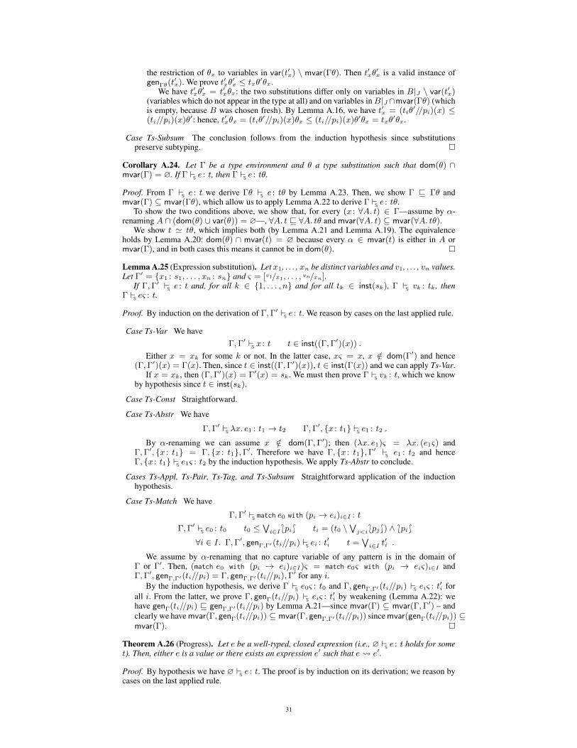
the restriction of θx to variables in var(t′x) \ mvar(Γθ). Then t′xθ′x is a valid instance ofgenΓθ(t

′x). We prove t′xθ′x ≤ txθ′θx.

We have t′xθ′x = t′xθx: the two substitutions differ only on variables in B|J \ var(t′x)(variables which do not appear in the type at all) and on variables inB|J∩mvar(Γθ) (whichis empty, because B was chosen fresh). By Lemma A.16, we have t′x = (tiθ

′//pi)(x) ≤(ti//pi)(x)θ′: hence, t′xθx = (tiθ

′//pi)(x)θx ≤ (ti//pi)(x)θ′θx = txθ′θx.

Case Ts-Subsum The conclusion follows from the induction hypothesis since substitutionspreserve subtyping.

Corollary A.24. Let Γ be a type environment and θ a type substitution such that dom(θ) ∩mvar(Γ) = ∅. If Γ

Se : t, then Γ

Se : tθ.

Proof. From ΓSe : t we derive Γθ

Se : tθ by Lemma A.23. Then, we show Γ v Γθ and

mvar(Γ) ⊆ mvar(Γθ), which allow us to apply Lemma A.22 to derive ΓSe : tθ.

To show the two conditions above, we show that, for every (x : ∀A. t) ∈ Γ—assume by α-renaming A ∩ (dom(θ) ∪ var(θ)) = ∅—, ∀A. t v ∀A. tθ and mvar(∀A. t) ⊆ mvar(∀A. tθ).

We show t ' tθ, which implies both (by Lemma A.21 and Lemma A.19). The equivalenceholds by Lemma A.20: dom(θ) ∩ mvar(t) = ∅ because every α ∈ mvar(t) is either in A ormvar(Γ), and in both cases this means it cannot be in dom(θ).

Lemma A.25 (Expression substitution). Let x1, . . . , xn be distinct variables and v1, . . . , vn values.Let Γ′ = x1 : s1, . . . , xn : sn and ς = [v1/x1, . . . , vn/xn].

If Γ,Γ′Se : t and, for all k ∈ 1, . . . , n and for all tk ∈ inst(sk), Γ

Svk : tk, then

ΓSeς : t.

Proof. By induction on the derivation of Γ,Γ′Se : t. We reason by cases on the last applied rule.

Case Ts-Var We haveΓ,Γ′

Sx : t t ∈ inst((Γ,Γ′)(x)) .

Either x = xk for some k or not. In the latter case, xς = x, x /∈ dom(Γ′) and hence(Γ,Γ′)(x) = Γ(x). Then, since t ∈ inst((Γ,Γ′)(x)), t ∈ inst(Γ(x)) and we can apply Ts-Var.

If x = xk, then (Γ,Γ′)(x) = Γ′(x) = sk. We must then prove ΓSvk : t, which we know

by hypothesis since t ∈ inst(sk).

Case Ts-Const Straightforward.

Case Ts-Abstr We have

Γ,Γ′Sλx. e1 : t1 → t2 Γ,Γ′, x : t1 S

e1 : t2 .

By α-renaming we can assume x /∈ dom(Γ,Γ′); then (λx. e1)ς = λx. (e1ς) andΓ,Γ′, x : t1 = Γ, x : t1,Γ′. Therefore we have Γ, x : t1,Γ′ S

e1 : t2 and henceΓ, x : t1 S

e1ς : t2 by the induction hypothesis. We apply Ts-Abstr to conclude.

Cases Ts-Appl, Ts-Pair, Ts-Tag, and Ts-Subsum Straightforward application of the inductionhypothesis.

Case Ts-Match We have

Γ,Γ′Smatch e0 with (pi → ei)i∈I : t

Γ,Γ′Se0 : t0 t0 ≤

∨i∈I*pi+ ti = (t0 \

∨j<i*pj+) ∧ *pi+

∀i ∈ I. Γ,Γ′, genΓ,Γ′(ti//pi) Sei : t

′i t =

∨i∈I t

′i .

We assume by α-renaming that no capture variable of any pattern is in the domain ofΓ or Γ′. Then, (match e0 with (pi → ei)i∈I)ς = match e0ς with (pi → eiς)i∈I andΓ,Γ′, genΓ,Γ′(ti//pi) = Γ, genΓ,Γ′(ti//pi),Γ

′ for any i.By the induction hypothesis, we derive Γ

Se0ς : t0 and Γ, genΓ,Γ′(ti//pi) S

eiς : t′i forall i. From the latter, we prove Γ, genΓ(ti//pi) S

eiς : t′i by weakening (Lemma A.22): wehave genΓ(ti//pi) v genΓ,Γ′(ti//pi) by Lemma A.21—since mvar(Γ) ⊆ mvar(Γ,Γ′) – andclearly we have mvar(Γ, genΓ(ti//pi)) ⊆ mvar(Γ, genΓ,Γ′(ti//pi)) since mvar(genΓ(ti//pi)) ⊆mvar(Γ).

Theorem A.26 (Progress). Let e be a well-typed, closed expression (i.e., ∅Se : t holds for some

t). Then, either e is a value or there exists an expression e′ such that e e′.

Proof. By hypothesis we have ∅Se : t. The proof is by induction on its derivation; we reason by

cases on the last applied rule.

31

Case Ts-Var This case does not occur because variables are not closed.

Case Ts-Const In this case e is a constant c and therefore a value.

Case Ts-Abstr In this case e is an abstraction λx. e1. Since it is also closed, it is a value.

Case Ts-Appl We have

∅Se1 e2 : t ∅

Se1 : t′ → t ∅

Se2 : t′ .

By the induction hypothesis, each of e1 and e2 either is a value or may reduce. If e1 e′1,then e1 e2 e′1 e2. If e1 is a value and e2 e′2, then e1 e2 e1 e

′2.

If both are values then, by Lemma A.12, e1 has the form λx. e3 for some e3. Then, we canapply R-Appl and e1 e2 e3[e2/x].

Case Ts-Pair We have

∅S

(e1, e2) : t1 × t2 ∅Se1 : t1 ∅

Se2 : t2 .

By the induction hypothesis, each of e1 and e2 either is a value or may reduce. If e1 e′1,then (e1, e2) (e′1, e2). If e1 is a value and e2 e′2, then (e1, e2) (e1, e

′2). If both are

values, then (e1, e2) is also a value.

Case Ts-Tag We have∅

Stag(e1) : tag(t1) ∅

Se1 : t1 .

Analogously to the previous case, by the induction hypothesis we have that either e1 isa value or e1 e′1. In the former case, tag(e1) is a value as well. In the latter, we havetag(e1) tag(e′1).

Case Ts-Match We have

∅Smatch e0 with (pi → ei)i∈I : t ∅

Se0 : t0 t0 ≤

∨i∈I*pi+ .

By the inductive hypothesis, either e0 is a value or it may reduce. In the latter case, ife0 e′0, then match e0 with (pi → ei)i∈I match e′0 with (pi → ei)i∈I .

If e0 is a value, on the other hand, the expression may reduce by application of R-Match.Since t0 ≤

∨i∈I*pi+, ∅

Se0 :

∨i∈I*pi+ holds by subsumption. Hence, since e0 is a value,

∅Se0 : *pi+ holds for at least one i (by Lemma A.13); for each such i we have e0/pi = ςi

(by Lemma A.15). Let j be the least of these i; then match e0 with (pi → ei)i∈I ejςj .

Case Ts-Subsum Straightforward application of the induction hypothesis.

Theorem A.27 (Subject reduction). Let e be an expression and t a type such that ΓSe : t. If

e e′, then ΓSe′ : t.

Proof. By induction on the derivation of ΓSe : t. We reason by cases on the last applied rule.

Cases Ts-Var, Ts-Const, and Ts-Abstr These cases do not occur: variables, constants, andabstractions never reduce.

Case Ts-Appl We have

ΓSe1 e2 : t Γ

Se1 : t′ → t Γ

Se2 : t′ .

e1 e2 e′ occurs in any of three ways: (i) e1 e′1 and e′ = e′1 e2; (ii) e1 is a value,e2 e′2 and e′ = e1 e

′2; (iii) both e1 and e2 are values, e1 is of the form λx. e3, and

e′ = e3[e2/x].In the first case, we derive by the induction hypothesis that Γ

Se′1 : t′ → t and conclude by

applying Ts-Appl again. The second case is analogous.In the third case, we know by Lemma A.12 that Γ, x : t′

Se3 : t. We also know that e2 is

a value such that ΓSe2 : t′. Then, by Lemma A.25, Γ

Se3[e2/x] : t.

Case Ts-Pair We have

ΓS

(e1, e2) : t1 × t2 ΓSe1 : t1 Γ

Se2 : t2 .

(e1, e2) e′ occurs either because e1 e′1 and e′ = (e′1, e2), or because e1 is a value,e2 e′2, and e′ = (e1, e

′2). In either case, the induction hypothesis allows us to derive that

the type of the component that reduces is preserved; therefore, we can apply Ts-Pair again toconclude.

Case Ts-Tag Analogously to the previous case, a variant expression only reduces if its argumentdoes, so we apply the induction hypothesis and Ts-Tag to conclude.

32

R-FixY (λx. e) e[Y (λx. e)/x]

Tk-FixK; Γ

Ke : τ → τ

K; ΓKY e : τ

Ts-FixΓ

Se : t→ t

ΓSY e : t

Figure 11. Rules for the fixed-point combinator.

Case Ts-Match We have

ΓSmatch e0 with (pi → ei)i∈I : t

ΓSe0 : t0 t0 ≤

∨i∈I*pi+ ti = (t0 \

∨j<i*pj+) ∧ *pi+

∀i ∈ I. Γ, genΓ(ti//pi) Sei : t

′i t =

∨i∈I t

′i .

The reduction match e0 with (pi → ei)i∈I e′ occurs either because e0 e′0 ande′ = match e′0 with (pi → ei)i∈I or because e0 is a value and e′ = ejς , where e0/pj = ς and,for all i < j, e0/pi = Ω. In the former case, we apply the induction hypothesis and concludeby Ts-Match.

In the latter case, ς is a substitution from the capture variables of pj to values. We can derive

ΓSe0 : *pj+ ∀i < j. Γ

Se0 : ¬*pi+

by Lemma A.15 and thence ΓSe0 : tj by Lemma A.14. Therefore, by Lemma A.17, we have

that, for all x ∈ capt(pj), ΓSxς : (tj//pj)(x). Let Γ′ = tj//pj .

We show that, additionally, ΓSxς : tx holds for every tx ∈ inst(genΓ(Γ′(x))). Every such

tx is equal to Γ′(x)θ for a θ such that dom(θ) ⊆ var(Γ′(x))\mvar(Γ). Then, ΓSxς : Γ′(x)θ

holds by Corollary A.24, since dom(θ) ∩mvar(Γ) = ∅ (the substitution does not change anymeaningful variable of Γ).

From Γ, genΓ(Γ′)Sej : t′j and from the fact that we have Γ

Sxς : tx for all x ∈ capt(pj)

and all tx ∈ inst(genΓ(Γ′(x))), we derive ΓSejς : t′j by Lemma A.25 and then conclude by

subsumption.

Case Ts-Subsum Straightforward application of the induction hypothesis.

Corollary A.28 (Type soundness). Let e be a well-typed, closed expression, that is, such that∅

Se : t holds for some t. Then, either e diverges or it reduces to a value v such that ∅

Sv : t.

Proof. Consequence of Theorem A.26 and Theorem A.27.

A.3.3 Completeness of S with respect to K

In the proof of completeness, we consider a calculus and type systems extended with the additionof a fixed-point combinator Y: this simplifies the proof (as it allows us to assume that all arrowtypes are inhabited) and it would be desirable anyway in order to use the system in pratice. We adda new production Y e to the grammar defining expressions, a new production YE to the grammarof evaluation contexts, and the new reduction rule R-Fix in Figure 11. We extend K and S with theaddition, respectively, of the rules Tk-Fix and Ts-Fix in Figure 11.

As mentioned in Section 4.3, we prove completeness of S with respect to K using inductivetechniques which do not account for the presence of recursion in kinds: we therefore have to restrictourselves to only consider kinding environments which do not feature recursion, (the non-recursiveenvironments defined below). We conjecture that coinductive techniques could be used instead toprove the result for general kinding environments.

Definition A.35 (Non-recursive kinding environments). We say that a kinding environment K isnon-recursive if, for all α such that K(α) = (L,U, T ), we have α /∈

⋃tag : τ∈T varK(τ).

Definition A.36. We define a function w which, given a k-type τ in a non-recursive kindingenvironment K, yields the measure w(τ,K) of τ in K. It is defined by the following equations.

w(α,K) =

1 +

∑tag : τ∈T w(τ,K) if K(α) = (L,U, T )

1 otherwise

w(b,K) = 1

w(τ1 → τ2,K) = w(τ1,K) + w(τ2,K) + 1

w(τ1 × τ2,K) = w(τ1,K) + w(τ2,K) + 1

Definition A.37 (Translation of types). Given a k-type τ in a non-recursive kinding environmentK, its translation is the s-type JτKK defined inductively by the rules in Figure 12.

33

JαKK =

α if K(α) = •(lowK(L, T ) ∨ α) ∧ uppK(U, T ) if K(α) = (L,U, T )

JbKK = b

Jτ1 → τ2KK = Jτ1KK → Jτ2KKJτ1 × τ2KK = Jτ1KK × Jτ2KK

where:

lowK(L, T ) =∨

tag∈L tag(∧

tag : τ∈T JτKK)

uppK(U, T ) =

∨tag∈U tag(

∧tag : τ∈T JτKK) if U 6= L∨

tag∈dom(T ) tag(∧

tag : τ∈T JτKK) ∨ (1V \∨

tag∈dom(T ) tag(1)) if U = L

Figure 12. Translation of k-types to s-types.

We define the translation of type schemes as J∀A.K′ . τKK = ∀A. JτKK,K′ and of typeenvironments by translating each type scheme pointwise.

Lemma A.29. For any k-type τ in a non-recursive kinding environment K, we have var(JτKK) ⊆varK(τ). Likewise, for any k-scheme σ and k-type environment Γ, we have var(JσKK) ⊆ varK(σ)and var(JΓKK) ⊆ varK(Γ).

Proof. The translation does not introduce new variables, therefore we can show var(JτKK) ⊆varK(τ) by induction on w(τ,K). We extend this straightforwardly to type schemes and envi-ronments.

Lemma A.30. Let p be a pattern and t ≤ *p+ an s-type. If K ` p : τ ⇒ Γ and t ≤ JτKK , then,for all x ∈ capt(p), (t//p)(x) ≤ JΓ(x)KK .

Proof. By structural induction on p.

Cases p = and p = c There is nothing to prove since capt(p) = ∅.

Case p = x We haveK ` p : τ ⇒ x : τ t//x = x : t

and must prove x : t(x) ≤ Jx : τ(x)KK , that is, t ≤ JτKK , which is true by hypothesis.

Case p = (p1, p2) We have

K ` p : τ1 × τ2 ⇒ Γ Γ = Γ1 ∪ Γ2 ∀i. K ` pi : τi ⇒ Γi

t//p = π1(t)//p1 ∪ π2(t)//p2 .

Since t ≤ Jτ1KK × Jτ2KK , by Property A.31 we have πi(t) ≤ JτiKK . Likewise, πi(t) ≤*pi+. We apply the induction hypothesis to conclude.

Case p = tag(p1) We have

K ` p : α⇒ Γ K ` p1 : τ1 ⇒ Γ

K(α) = (L,U, T ) ( tag ∈ U implies tag : τ1 ∈ T ) t//p = π tag(t)//p1 .

Since t ≤ * tag(p1)+ = tag(*p1+), by Property A.32 we have π tag(t) ≤ *p1+. We nextprove π tag(t) ≤ Jτ1KK , which allows us to apply the induction hypothesis and conclude.

The translation of α is JαKK = (lowK(L, T ) ∨ α) ∧ uppK(U, T ). We have t ≤ JαKKand hence t ≤ uppK(U, T ). Since t ≤ tag(1), t ≤ uppK(U, T ) ∧ tag(1). We distribute theintersection over the summands of uppK(U, T ), which is a union.

If tag /∈ U (in which case U 6= L), then all summands have the form tag1(τ ′) and for eachtag1 we have tag1 6= tag: hence, the intersection is empty and thus we have t ≤ 0 ' tag(0).

Then π tag(t) ≤ 0 ≤ Jτ1KK .If tag ∈ U , then necessarily tag ∈ dom(T ) holds as well. In that case the intersection

uppK(U, T )∧ tag(1) is equivalent to tag(∧

tag : τ ′∈T Jτ ′KK). Hence t ≤ tag(∧

tag : τ ′∈T Jτ ′KK)

and π tag(t) ≤∧

tag : τ ′∈T Jτ ′KK . Since tag : τ1 ∈ T ,∧

tag : τ ′∈T Jτ ′KK ≤ Jτ1KK , from whichfollows π tag(t) ≤ Jτ1KK .

Case p = p1&p2 We directly apply the induction hypothesis to both sub-patterns and conclude.

34

Case p = p1|p2 We have

K ` p : τ ⇒ Γ ∀i. K ` pi : τ ⇒ Γ

t//p = (t ∧ *p1+)//p1 ∨∨ (t \ *p1+)//p2 .

Since t ∧ *p1+ and t \ *p1+ are subtypes of t, they are also subtypes of JτKK . We can applythe induction hypothesis and, for each x, derive both that (t ∧ *p1+//p1)(x) ≤ JΓ(x)KK andthat (t \ *p1+//p2)(x) ≤ JΓ(x)KK . Hence, (t//p)(x) ≤ JΓ(x)KK .

Lemma A.31 (Translation of type substitutions). LetK,K′ be two non-recursive kinding environ-ments such that dom(K′) ∩ (dom(K) ∪ var∅(K)) = ∅. Let θ be a k-type substitution such thatdom(θ) ⊆ dom(K′) and K,K′ ` θ : K.

Let θ′ be the s-type substitution defined as [ JαθKK/α | α ∈ dom(K′) ]. For every k-type τ , wehave JτKK,K′θ′ ' JτθKK .

Proof. By complete induction on w(τ, (K,K′)). We proceed by cases on τ and assume that thelemma holds for all τ ′ such that w(τ ′, (K,K′)) < w(τ, (K,K′)).

Case τ = α, with (K,K′)(α) = • We have JαKK,K′ = α, hence JαKK,K′θ′ = αθ′. Eitherα ∈ dom(K) or α ∈ dom(K′) (the domains are disjoint). In the former case, αθ = α andαθ′ = α. Thus we have JαKK,K′θ′ = α = JαθKK . In the latter, αθ′ = JαθKK holds bydefinition of θ′.

Case τ = α, with K(α) = (L,U, T ) and α /∈ dom(K′) We have JαKK,K′ = JαKK because novariable in the kind of α is in dom(K′). For the same reason, since the translation does not addvariables, JαKK,K′θ′ = JαKK . Additionally, αθ = α, so also JαθKK = JαKK .

Case τ = α, with K′(α) = (L′, U ′, T ′) Because K,K′ ` θ : K, we know that αθ is somevariable β such that K(β) = (L,U, T ) and (L,U, T ) (L′, U ′, T ′θ).

We haveJαθKK = JβKK = (lowK(L, T ) ∨ β) ∧ uppK(U, T )

and

JαKK,K′θ′ =((lowK,K′(L′, T ′) ∨ α) ∧ uppK,K′(U

′, T ′))θ′

= (lowK,K′(L′, T ′)θ′ ∨ αθ′) ∧ uppK,K′(U′, T ′)θ′

=(lowK,K′(L′, T ′)θ′ ∨

((lowK(L, T ) ∨ β) ∧ uppK(U, T )

))∧ uppK,K′(U

′, T ′)θ′ .

Let us define

l = lowK(L, T ) u = uppK(U, T )

l′ = lowK,K′(L′, T ′)θ′ u′ = uppK,K′(U′, T ′)θ′

and assume that the following hold (we prove them below):

l ≤ u l′ ≤ u′ l′ ≤ l u ≤ u′ .

Then we have also l′ ≤ u by transitivity. Whenever t ≤ t′, we have t ∧ t′ ' t and t ∨ t′ ' t′.Thus we have the following equivalences:

JαKK,K′θ′ = (l′ ∨ ((l ∨ β) ∧ u)) ∧ u′

' (l′ ∧ u′) ∨ ((l ∨ β) ∧ u ∧ u′) distributivity

' l′ ∨ ((l ∨ β) ∧ u) l′ ≤ u′ and u ≤ u′

' (l′ ∨ l ∨ β) ∧ (l′ ∨ u) distributivity

' (l ∨ β) ∧ u l′ ≤ l and l′ ≤ uby which we conclude.

We now prove our four assumptions. The first, l ≤ u, holds because L ⊆ U andL ⊆ dom(T ): hence each branch of l appears in u as well. The second is analogous.

For the other assumptions, note that Jτ ′KK,K′θ′ ' Jτ ′θKK holds for all τ ′ in the range ofT ′. To prove l′ ≤ l, note that L′ ⊆ L and T ′θ ⊆ T . In l′, we distribute the application ofθ′ over all the summands of the union and inside all variant type constructors. Then, we showtag(

∧tag : τ ′∈T ′Jτ ′KK,K′θ′) ≤ l for each tag ∈ L′. We have tag(

∧tag : τ ′∈T ′Jτ ′KK,K′θ′) '

tag(∧

tag : τ ′∈T ′Jτ ′θKK) = tag(∧

tag : τ ′θ∈T ′θJτ′θKK). Since L′ ⊆ L, there is a summand of

l with the same tag. Since tag is in the lower bound, it has a single type in both T and T ′ and,since T ′θ ⊆ T , the type it has in T must be τ ′θ.

To prove u ≤ u′, note that U ⊆ U ′. If U = L, then U ′ = L. Then both u and u′ are unionsof two types: the union of tags mentioned respectively in T and T ′ and the rest. For each tag, if

35

tag /∈ dom(T ), then tag /∈ dom(T ′), in which case both u and u′ admit it with any argumenttype. If tag ∈ dom(T ), either tag ∈ dom(T ′) or not. In the former case, u admits a smallerargument type than u′ because T ′θ ⊆ T . The same occurs in the latter case, since u′ admitstag with any argument type.

If U 6= L, then U ′ could be L or not. In either case we can prove, for each tag ∈ U , that u′

admits tag with a larger argument type than u does.

Case τ = b Straightforward, since a basic type is translated into itself and is never affected bysubstitutions.

Case τ = τ1 → τ2 By the induction hypothesis we have JτiKK,K′θ′ ' JτiθKK for both i. Then

Jτ1 → τ2KK,K′θ′ = (Jτ1KK,K′θ′)→ (Jτ2KK,K′θ′) ' Jτ1θKK → Jτ2θKK= J(τ1θ)→ (τ2θ)KK = J(τ1 → τ2)θKK .

Case τ = τ1 × τ2 Analogous to the previous case.

Lemma A.32. If ∅Sv : JτKK , then there exists a value v′ such that K;∅

Kv′ : τ and, for every

pattern p, v/p = Ω ⇐⇒ v′/p = Ω.

Proof. By structural induction on v.Note that values are always typed by an application of the typing rule corresponding to

their form (Ts-Const, Ts-Abstr, Ts-Pair, or Ts-Tag) to appropriate premises, possibly followed byapplications of Ts-Subsum. Hence, if ∅

Sv : t, there is a type t′ ≤ t such that ∅

Sv : t′ and that

the last typing rule used to derive ∅Sv : t′ is one of the four above, given by the form of v.

Case v = c We have JτKK ≥ c. Hence τ = bc, as the translation of any other τ is disjoint fromc. Then we can take v′ = v.

Case v = (v1, v2) We have JτKK ≥ t1 × t2 for some t1 and t2. Hence τ = τ1 × τ2: any otherτ would translate to a type disjoint from all products. Therefore ∅

Sv : Jτ1KK × Jτ2KK . By

Lemma A.12 we have ∅Svi : JτiKK for both i; then by the induction hypothesis we find v′i

for both i and let v′ = (v′1, v′2).

Case v = tag(v1) We have JτKK ≥ tag(t1) and ∅Sv : tag(t1) for some t1 0 (since t1

types the value v1). Therefore, by the same reasoning as above, τ = α withK(α) = (L,U, T ).Since JτKK ≥ tag(t1), we have tag ∈ L and therefore tag : τ1 ∈ T for some τ1 such thatt1 ≤ Jτ1KK . Then we have ∅

Sv1 : Jτ1KK ; we may apply the induction hypothesis to find a

value v′1 and let v′ = tag(v′1).

Case v = λx. e Note that an abstraction is only accepted by patterns which accept any value, soany two abstractions fail to match exactly the same patterns.

We have ∅Sv : t1 → t2 for some t1 → t2 ≤ JτKK . Hence we know τ is of the

form τ1 → τ2; thus we have ∅Sv : Jτ1KK → Jτ2KK . We take v′ to be the function

λx. Y (λf. λx. f x) x, which never terminates and can be assigned any arrow type.

Lemma A.33. Let K be a kinding environment, τ a k-type, and P a set of patterns. If τ 4K P ,then JτKK ≤

∨p∈P *p+.

Proof. By contradiction, assume that τ 4K P holds but JτKK ∨p∈P *p+. The latter condition

implies that there exists a value v in the interpretation of JτKK which is not in the interpretationof∨p∈P *p+. Because the definition of accepted type is exact with respect to the semantics of

pattern matching, we have v/p = Ω for all p ∈ P . We also have ∅Sv : JτKK since v is in

the interpretation of that type (typing is complete with respect to the interpretation if we restrictourselves to translations of k-types).

By Lemma A.32, from v we can build a value v′ such that K;∅Kv′ : τ and, for every pattern

p, v/p = Ω ⇐⇒ v′/p = Ω. We reach a contradiction, since τ 4K P and K;∅Kv′ : τ imply

that there exists a p ∈ P such that v′/p 6= Ω, whereas we have v/p = Ω for all p ∈ P .

Theorem A.34 (Preservation of typing). Let e be an expression, K a non-recursive kindingenvironment, Γ a k-type environment, and τ a k-type. If K; Γ

Ke : τ , then JΓKK S

e : JτKK .

Proof. By induction on the derivation of K; ΓKe : τ . We reason by cases on the last applied rule.

Case Tk-Var We have

K; ΓKx : τ τ ∈ instK(Γ(x)) hence

Γ(x) = ∀A.Kx . τx τ = τxθ dom(θ) ⊆ A K,Kx ` θ : K

36

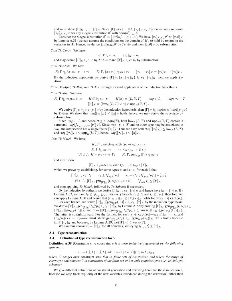
and must show JΓKK Sx : JτKK . Since JΓKK(x) = ∀A. JτxKK,Kx , by Ts-Var we can derive

JτxKK,Kxθ′ for any s-type substitution θ′ with dom(θ′) ⊆ A.

Consider the s-type substitution θ′ = [ JαθKK/α | α ∈ A ]. We have JτxKK,Kxθ′ ' JτxθKK

by Lemma A.31 (we can assume the conditions on the domain of Kx to hold by renaming thevariables in A). Hence, we derive JτxKK,Kxθ

′ by Ts-Var and then JτxθKK by subsumption.

Case Tk-Const We haveK; Γ

Kc : bc JbcKK = bc

and may derive JΓKK Sc : c by Ts-Const and JΓKK S

c : bc by subsumption.

Case Tk-Abstr We have

K; ΓKλx. e1 : τ1 → τ2 K; Γ, x : τ1 K

e1 : τ2 Jτ1 → τ2KK = Jτ1KK → Jτ2KK .

By the induction hypothesis we derive JΓKK , x : Jτ1KK Se1 : Jτ2KK , then we apply Ts-

Abstr.

Cases Tk-Appl, Tk-Pair, and Tk-Fix Straightforward application of the induction hypothesis.

Case Tk-Tag We have

K; ΓK

tag(e1) : α K; ΓKe1 : τ1 K(α) = (L,U, T ) tag ∈ L tag : τ1 ∈ T

JαKK = (lowK(L, T ) ∨ α) ∧ uppK(U, T ) .

We derive JΓKK Se1 : Jτ1KK by the induction hypothesis, then JΓKK S

tag(e1) : tag(Jτ1KK)by Ts-Tag. We show that tag(Jτ1KK) ≤ JαKK holds: hence, we may derive the supertype bysubsumption.

Since tag ∈ L and hence tag ∈ dom(T ), both lowK(L, T ) and uppK(U, T ) contain asummand tag(

∧tag : τ ′∈T Jτ ′KK). Since tag : τ1 ∈ T and no other type may be associated to

tag, the intersection has a single factor Jτ1KK . Thus we have both tag(Jτ1KK) ≤ lowK(L, T )and tag(Jτ1KK) ≤ uppK(U, T ); hence, tag(Jτ1KK) ≤ JαKK .

Case Tk-Match We have

K; ΓKmatch e0 with (pi → ei)i∈I : τ

K; ΓKe0 : τ0 τ0 4K pi | i ∈ I

∀i ∈ I. K ` pi : τ0 ⇒ Γi K; Γ, genK;Γ(Γi) Kei : τ

and must showJΓKK S

match e0 with (pi → ei)i∈I : JτKKwhich we prove by establishing, for some types t0 and ti, t′i for each i, that

JΓKK Se0 : t0 t0 ≤

∨i∈I*pi+ ti = (t0 \

∨j<i*pj+) ∧ *pi+

∀i ∈ I. JΓKK , genJΓKK (ti//pi) Sei : t

′i

∨i∈I t

′i ≤ JτKK .

and then applying Ts-Match, followed by Ts-Subsum if necessary.By the induction hypothesis we derive JΓKK S

e0 : Jτ0KK and hence have t0 = Jτ0KK . ByLemma A.33, we have t0 ≤

∨i∈I*pi+. For every branch, ti ≤ t0 and ti ≤ *pi+: therefore, we

can apply Lemma A.30 and derive that (ti//pi)(x) ≤ JΓi(x)KK holds for every x ∈ capt(pi).For each branch, we derive JΓKK , JgenK;Γ(Γi)KK S

ei : JτKK by the induction hypothesis.We derive JΓKK , genJΓKK (ti//pi) S

ei : JτKK by Lemma A.22 by proving JΓKK , genJΓKK (ti//pi) vJΓKK , JgenK;Γ(Γi)KK and mvar(JΓKK , genJΓKK (ti//pi)) ⊆ mvar(JΓKK , JgenK;Γ(Γi)KK).The latter is straightforward. For the former, for each x ∈ capt(pi)—say Γi(x) = τx and(ti//pi)(x) = tx—we must show genJΓKK (tx) v JgenK;Γ(τx)KK . This holds becausetx ≤ JτxKK and because, by Lemma A.29, var(JΓKK) ⊆ varK(Γ).

We can thus choose t′i = JτKK for all branches, satisfying∨i∈I t

′i ≤ JτKK .

A.4 Type reconstructionA.4.1 Definition of type reconstruction for S

Definition A.38 (Constraints). A constraint c is a term inductively generated by the followinggrammar:

c ::= t ≤ t | x ≤ t | def Γ in C | let [C](Γi in Ci)i∈I

where C ranges over constraint sets, that is, finite sets of constraints, and where the range ofevery type environment Γ in constraints of the form def or let only contains types (i.e., trivial typeschemes).

We give different definitions of constraint generation and rewriting here than those in Section 5,because we keep track explicitly of the new variables introduced during the derivation, rather than

37

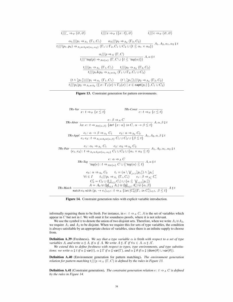
t/// ⇒∅ (∅,∅) t///x⇒∅ (x : t,∅) t///c⇒∅ (∅,∅)

α1///p1 ⇒A1 (Γ1, C1) α2///p2 ⇒A2 (Γ2, C2)

t///(p1, p2)⇒A1]A2]α1,α2 (Γ1 ∪ Γ2, C1 ∪ C2 ∪ t ≤ α1 × α2)A1, A2, α1, α2 ] t

α///p⇒A (Γ, C)

t/// tag(p)⇒A]α (Γ, C ∪ t ≤ tag(α))A,α ] t

t///p1 ⇒A1 (Γ1, C1) t///p2 ⇒A2 (Γ2, C2)

t///p1&p2 ⇒A1]A2 (Γ1 ∪ Γ2, C1 ∪ C2)

(t ∧ *p1+)///p1 ⇒A1 (Γ1, C1) (t \ *p1+)///p2 ⇒A2 (Γ2, C2)

t///p1|p2 ⇒A1]A2 (x : Γ1(x) ∨ Γ2(x) | x ∈ capt(p1) , C1 ∪ C2)

Figure 13. Constraint generation for pattern environments.

TRs-Varx : t⇒∅ x ≤ t

TRs-Constc : t⇒∅ c ≤ t

TRs-Abstre : β ⇒A C

λx. e : t⇒A]α,β def x : α in C, α→ β ≤ tA,α, β ] t

TRs-Apple1 : α→ β ⇒A1 C1 e2 : α⇒A2 C2

e1 e2 : t⇒A1]A2]α,β C1 ∪ C2 ∪ β ≤ tA1, A2, α, β ] t

TRs-Paire1 : α1 ⇒A1 C1 e2 : α2 ⇒A2 C2

(e1, e2) : t⇒A1]A2]α1,α2 C1 ∪ C2 ∪ α1 × α2 ≤ tA1, A2, α1, α2 ] t

TRs-Tage : α⇒A C

tag(e) : t⇒A]α C ∪ tag(α) ≤ tA,α ] t

TRs-Match

e0 : α⇒A0 C0 ti = (α \∨j<i*pj+) ∧ *pi+

∀i ∈ I ti///pi ⇒Ai (Γi, Ci) ei : β ⇒A′iC′i

C′0 = C0 ∪ (⋃i∈I Ci) ∪ α ≤

∨i∈I*pi+

A = A0 ] (⊎i∈I Ai) ] (

⊎i∈I A

′i) ] α, β

match e0 with (pi → ei)i∈I : t⇒A let [C′0](Γi in C′i)i∈I , β ≤ t

A ] t

Figure 14. Constraint generation rules with explicit variable introduction.

informally requiring them to be fresh. For instance, in e : t ⇒A C, A is the set of variables whichappear in C but not in t. We will omit it for soundness proofs, where it is not relevant.

We use the symbol] to denote the union of two disjoint sets. Therefore, when we writeA1]A2,we require A1 and A2 to be disjoint. When we require this for sets of type variables, the conditionis always satisfiable by an appropriate choice of variables, since there is an infinite supply to choosefrom.

Definition A.39 (Freshness). We say that a type variable α is fresh with respect to a set of typevariables A, and write α ] A, if α /∈ A. We write A ] A′ if ∀α ∈ A. α ] A′.

We extend this to define freshness with respect to types, type environments, and type substitu-tions: we write α ] t if α ] var(t), α ] Γ if α ] var(Γ), and α ] θ if α ] (dom(θ) ∪ var(θ)).

Definition A.40 (Environment generation for pattern matching). The environment generationrelation for pattern matching t///p⇒A (Γ, C) is defined by the rules in Figure 13.

Definition A.41 (Constraint generation). The constraint generation relation e : t⇒A C is definedby the rules in Figure 14.

38

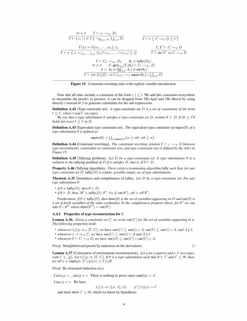
∀i ∈ I Γ ` ci Ai Di

Γ ` ci | i ∈ I ⊎i∈I Ai

⋃i∈I Di Γ ` t ≤ t′ ∅ t ≤ t′

Γ(x) = ∀α1, . . . , αn. txΓ ` x ≤ t β1,...,βn tx[β1/α1, . . . , βn/αn] ≤ t

Γ,Γ′ ` C A D

Γ ` def Γ′ in C A D

Γ ` C0 A0 D0 θ0 ∈ tally(D0)∀i ∈ I Γ, genΓθ0

(Γiθ0) ` Ci Ai DiA = A0 ] (

⊎i∈I Ai) ] var(θ0)

Γ ` let [C0](Γi in Ci)i∈I A equiv(θ0) ∪⋃i∈I Di

Figure 15. Constraint rewriting rules with explicit variable introduction.

Note that all rules include a constraint of the form (·) ≤ t. We add this constraint everywhereto streamline the proofs; in practice, it can be dropped from TRs-Appl and TRs-Match by usingdirectly t instead of β to generate constraints for the sub-expressions.

Definition A.42 (Type-constraint set). A type-constraint set D is a set of constraints of the formt ≤ t′, where t and t′ are types.

We say that a type substitution θ satisfies a type-constraint set D, written θ D, if tθ ≤ t′θholds for every t ≤ t′ in D.

Definition A.43 (Equivalent type-constraint set). The equivalent type-constraint set equiv(θ) of atype substitution θ is defined as

equiv(θ) =⋃α∈dom(θ)α ≤ αθ, αθ ≤ α .

Definition A.44 (Constraint rewriting). The constraint rewriting relation Γ ` c A D betweentype environments, constraints or constraint sets, and type-constraint sets is defined by the rules inFigure 15.

Definition A.45 (Tallying problem). Let D be a type-constraint set. A type substitution θ is asolution to the tallying problem of D if it satisfies D, that is, if θ D.

Property A.46 (Tallying algorithm). There exists a terminating algorithm tally such that, for anytype-constraint set D, tally(D) is a finite, possibly empty, set of type substitutions.

Theorem A.35 (Soundness and completeness of tally). Let D be a type-constraint set. For anytype substitution θ:

• if θ ∈ tally(D), then θ D;• if θ D, then ∃θ′ ∈ tally(D), θ′′. ∀α /∈ var(θ′). αθ ' αθ′θ′′.

Furthermore, if θ ∈ tally(D), then dom(θ) is the set of variables appearing in D and var(θ) isa set of fresh variables of the same cardinality. In the completeness property above, for θ′′ we cantake θ ∪ θ′′′ where dom(θ′′′) = var(θ′).

A.4.2 Properties of type reconstruction for S

Lemma A.36. Given a constraint set C, we write var(C) for the set of variables appearing in it.The following properties hold:

• whenever t///p⇒A (Γ, C), we have var(C) ⊆ var(t) ∪A, var(Γ) ⊆ var(t) ∪A, and A ] t;• whenever e : t⇒A C, we have var(C) ⊆ var(t) ∪A and A ] t;• whenever Γ ` C A D, we have var(D) ⊆ var(C) ∪ var(Γ) ∪A.

Proof. Straightforward proofs by induction on the derivations.

Lemma A.37 (Correctness of environment reconstruction). Let p be a pattern and t, t′ two types,with t′ ≤ *p+. Let t///p ⇒ (Γ, C). If θ is a type substitution such that θ C and t′ ≤ tθ, then,for all x ∈ capt(p), (t′//p)(x) ≤ Γ(x)θ.

Proof. By structural induction on p.

Cases p = and p = c There is nothing to prove since capt(p) = ∅.

Case p = x We havet///x⇒ (x : t,∅) (t′//x)(x) = t′

and must show t′ ≤ tθ, which we know by hypothesis.

39

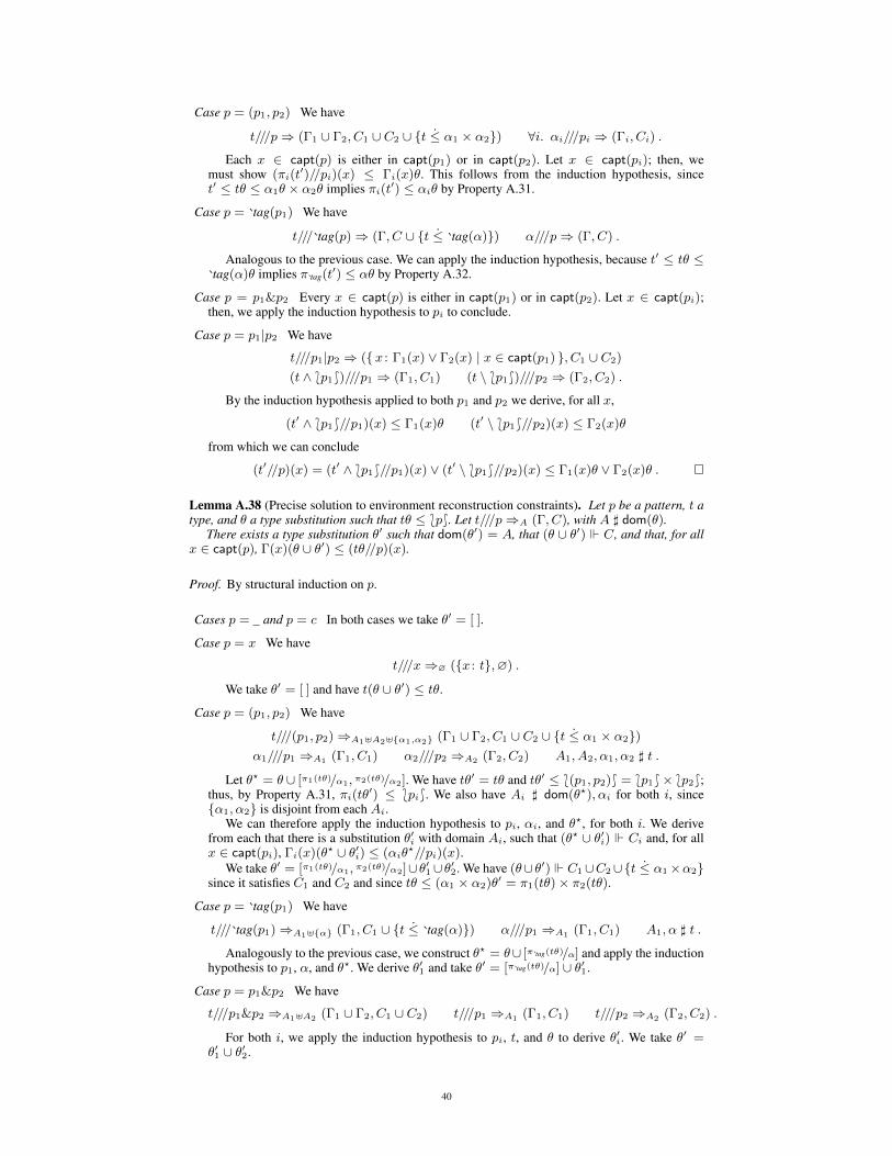
Case p = (p1, p2) We have

t///p⇒ (Γ1 ∪ Γ2, C1 ∪ C2 ∪ t ≤ α1 × α2) ∀i. αi///pi ⇒ (Γi, Ci) .

Each x ∈ capt(p) is either in capt(p1) or in capt(p2). Let x ∈ capt(pi); then, wemust show (πi(t

′)//pi)(x) ≤ Γi(x)θ. This follows from the induction hypothesis, sincet′ ≤ tθ ≤ α1θ × α2θ implies πi(t′) ≤ αiθ by Property A.31.

Case p = tag(p1) We have

t/// tag(p)⇒ (Γ, C ∪ t ≤ tag(α)) α///p⇒ (Γ, C) .

Analogous to the previous case. We can apply the induction hypothesis, because t′ ≤ tθ ≤tag(α)θ implies π tag(t

′) ≤ αθ by Property A.32.

Case p = p1&p2 Every x ∈ capt(p) is either in capt(p1) or in capt(p2). Let x ∈ capt(pi);then, we apply the induction hypothesis to pi to conclude.

Case p = p1|p2 We have

t///p1|p2 ⇒ (x : Γ1(x) ∨ Γ2(x) | x ∈ capt(p1) , C1 ∪ C2)

(t ∧ *p1+)///p1 ⇒ (Γ1, C1) (t \ *p1+)///p2 ⇒ (Γ2, C2) .

By the induction hypothesis applied to both p1 and p2 we derive, for all x,

(t′ ∧ *p1+//p1)(x) ≤ Γ1(x)θ (t′ \ *p1+//p2)(x) ≤ Γ2(x)θ

from which we can conclude

(t′//p)(x) = (t′ ∧ *p1+//p1)(x) ∨ (t′ \ *p1+//p2)(x) ≤ Γ1(x)θ ∨ Γ2(x)θ .

Lemma A.38 (Precise solution to environment reconstruction constraints). Let p be a pattern, t atype, and θ a type substitution such that tθ ≤ *p+. Let t///p⇒A (Γ, C), with A ] dom(θ).

There exists a type substitution θ′ such that dom(θ′) = A, that (θ ∪ θ′) C, and that, for allx ∈ capt(p), Γ(x)(θ ∪ θ′) ≤ (tθ//p)(x).

Proof. By structural induction on p.

Cases p = and p = c In both cases we take θ′ = [ ].

Case p = x We have

t///x⇒∅ (x : t,∅) .

We take θ′ = [ ] and have t(θ ∪ θ′) ≤ tθ.

Case p = (p1, p2) We have

t///(p1, p2)⇒A1]A2]α1,α2 (Γ1 ∪ Γ2, C1 ∪ C2 ∪ t ≤ α1 × α2)α1///p1 ⇒A1 (Γ1, C1) α2///p2 ⇒A2 (Γ2, C2) A1, A2, α1, α2 ] t .

Let θ? = θ ∪ [π1(tθ)/α1, π2(tθ)/α2]. We have tθ′ = tθ and tθ′ ≤ *(p1, p2)+ = *p1+× *p2+;thus, by Property A.31, πi(tθ′) ≤ *pi+. We also have Ai ] dom(θ?), αi for both i, sinceα1, α2 is disjoint from each Ai.

We can therefore apply the induction hypothesis to pi, αi, and θ?, for both i. We derivefrom each that there is a substitution θ′i with domain Ai, such that (θ? ∪ θ′i) Ci and, for allx ∈ capt(pi), Γi(x)(θ? ∪ θ′i) ≤ (αiθ

?//pi)(x).We take θ′ = [π1(tθ)/α1, π2(tθ)/α2]∪θ′1∪θ′2. We have (θ∪θ′) C1∪C2∪t ≤ α1×α2

since it satisfies C1 and C2 and since tθ ≤ (α1 × α2)θ′ = π1(tθ)× π2(tθ).

Case p = tag(p1) We have

t/// tag(p1)⇒A1]α (Γ1, C1 ∪ t ≤ tag(α)) α///p1 ⇒A1 (Γ1, C1) A1, α ] t .

Analogously to the previous case, we construct θ? = θ∪ [π tag(tθ)/α] and apply the inductionhypothesis to p1, α, and θ?. We derive θ′1 and take θ′ = [π tag(tθ)/α] ∪ θ′1.

Case p = p1&p2 We have

t///p1&p2 ⇒A1]A2 (Γ1 ∪ Γ2, C1 ∪ C2) t///p1 ⇒A1 (Γ1, C1) t///p2 ⇒A2 (Γ2, C2) .

For both i, we apply the induction hypothesis to pi, t, and θ to derive θ′i. We take θ′ =θ′1 ∪ θ′2.

40

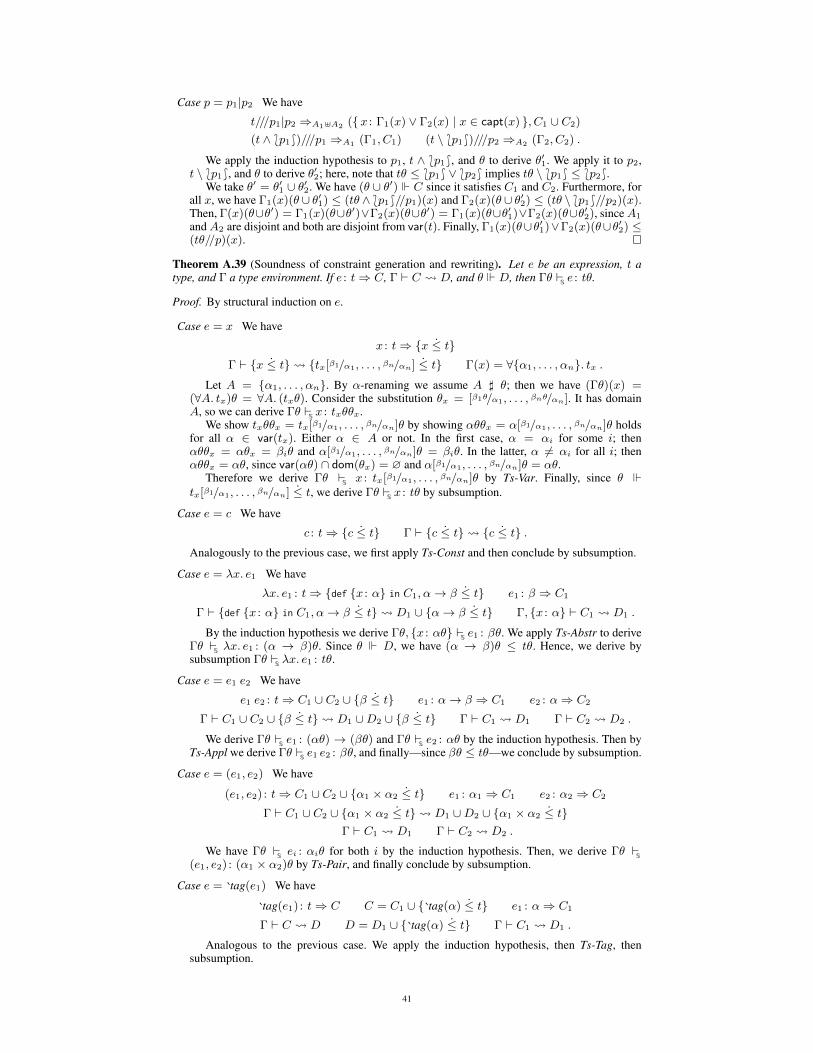
Case p = p1|p2 We have

t///p1|p2 ⇒A1]A2 (x : Γ1(x) ∨ Γ2(x) | x ∈ capt(x) , C1 ∪ C2)

(t ∧ *p1+)///p1 ⇒A1 (Γ1, C1) (t \ *p1+)///p2 ⇒A2 (Γ2, C2) .

We apply the induction hypothesis to p1, t ∧ *p1+, and θ to derive θ′1. We apply it to p2,t \ *p1+, and θ to derive θ′2; here, note that tθ ≤ *p1+ ∨ *p2+ implies tθ \ *p1+ ≤ *p2+.

We take θ′ = θ′1 ∪ θ′2. We have (θ ∪ θ′) C since it satisfies C1 and C2. Furthermore, forall x, we have Γ1(x)(θ ∪ θ′1) ≤ (tθ ∧ *p1+//p1)(x) and Γ2(x)(θ ∪ θ′2) ≤ (tθ \ *p1+//p2)(x).Then, Γ(x)(θ∪θ′) = Γ1(x)(θ∪θ′)∨Γ2(x)(θ∪θ′) = Γ1(x)(θ∪θ′1)∨Γ2(x)(θ∪θ′2), sinceA1

andA2 are disjoint and both are disjoint from var(t). Finally, Γ1(x)(θ∪θ′1)∨Γ2(x)(θ∪θ′2) ≤(tθ//p)(x).

Theorem A.39 (Soundness of constraint generation and rewriting). Let e be an expression, t atype, and Γ a type environment. If e : t⇒ C, Γ ` C D, and θ D, then Γθ

Se : tθ.

Proof. By structural induction on e.

Case e = x We have

x : t⇒ x ≤ tΓ ` x ≤ t tx[β1/α1, . . . , βn/αn] ≤ t Γ(x) = ∀α1, . . . , αn. tx .

Let A = α1, . . . , αn. By α-renaming we assume A ] θ; then we have (Γθ)(x) =(∀A. tx)θ = ∀A. (txθ). Consider the substitution θx = [β1θ/α1, . . . , βnθ/αn]. It has domainA, so we can derive Γθ

Sx : txθθx.

We show txθθx = tx[β1/α1, . . . , βn/αn]θ by showing αθθx = α[β1/α1, . . . , βn/αn]θ holdsfor all α ∈ var(tx). Either α ∈ A or not. In the first case, α = αi for some i; thenαθθx = αθx = βiθ and α[β1/α1, . . . , βn/αn]θ = βiθ. In the latter, α 6= αi for all i; thenαθθx = αθ, since var(αθ) ∩ dom(θx) = ∅ and α[β1/α1, . . . , βn/αn]θ = αθ.

Therefore we derive ΓθSx : tx[β1/α1, . . . , βn/αn]θ by Ts-Var. Finally, since θ

tx[β1/α1, . . . , βn/αn] ≤ t, we derive ΓθSx : tθ by subsumption.

Case e = c We have

c : t⇒ c ≤ t Γ ` c ≤ t c ≤ t .Analogously to the previous case, we first apply Ts-Const and then conclude by subsumption.

Case e = λx. e1 We have

λx. e1 : t⇒ def x : α in C1, α→ β ≤ t e1 : β ⇒ C1

Γ ` def x : α in C1, α→ β ≤ t D1 ∪ α→ β ≤ t Γ, x : α ` C1 D1 .

By the induction hypothesis we derive Γθ, x : αθSe1 : βθ. We apply Ts-Abstr to derive

ΓθSλx. e1 : (α → β)θ. Since θ D, we have (α → β)θ ≤ tθ. Hence, we derive by

subsumption ΓθSλx. e1 : tθ.

Case e = e1 e2 We have

e1 e2 : t⇒ C1 ∪ C2 ∪ β ≤ t e1 : α→ β ⇒ C1 e2 : α⇒ C2

Γ ` C1 ∪ C2 ∪ β ≤ t D1 ∪D2 ∪ β ≤ t Γ ` C1 D1 Γ ` C2 D2 .

We derive ΓθSe1 : (αθ) → (βθ) and Γθ

Se2 : αθ by the induction hypothesis. Then by

Ts-Appl we derive ΓθSe1 e2 : βθ, and finally—since βθ ≤ tθ—we conclude by subsumption.

Case e = (e1, e2) We have

(e1, e2) : t⇒ C1 ∪ C2 ∪ α1 × α2 ≤ t e1 : α1 ⇒ C1 e2 : α2 ⇒ C2

Γ ` C1 ∪ C2 ∪ α1 × α2 ≤ t D1 ∪D2 ∪ α1 × α2 ≤ tΓ ` C1 D1 Γ ` C2 D2 .

We have ΓθSei : αiθ for both i by the induction hypothesis. Then, we derive Γθ

S

(e1, e2) : (α1 × α2)θ by Ts-Pair, and finally conclude by subsumption.

Case e = tag(e1) We have

tag(e1) : t⇒ C C = C1 ∪ tag(α) ≤ t e1 : α⇒ C1

Γ ` C D D = D1 ∪ tag(α) ≤ t Γ ` C1 D1 .

Analogous to the previous case. We apply the induction hypothesis, then Ts-Tag, thensubsumption.

41

Case e = match e0 with (pi → ei)i∈I We have

match e0 with (pi → ei)i∈I : t⇒ C

C = let [C′0](Γi in C′i)i∈I , β ≤ t

C′0 = C0 ∪ (⋃i∈I Ci) ∪ α ≤

∨i∈I*pi+ e0 : α⇒ C0

∀i ∈ I ti = (α \∨j<i*pj+) ∧ *pi+ ti///pi ⇒ (Γi, Ci) ei : β ⇒ C′i

Γ ` C D

Γ ` C′0 D′0 Γ ` C0 D0 D′0 = D0 ∪ (⋃i∈I Ci) ∪ α ≤

∨i∈I*pi+

θ0 ∈ tally(D′0) ∀i ∈ I. Γ, genΓθ0(Γiθ0) ` C′i D′i

D = equiv(θ0) ∪ (⋃i∈I D

′i) ∪ β ≤ t

and we must show ΓθSmatch e0 with (pi → ei)i∈I : tθ.

We prove it by establishing, for some types t0 and ti, t′i for each i, that

ΓθSe0 : t0 t0 ≤

∨i∈I*pi+ ti = (t0 \

∨j<i*pj+) ∧ *pi+

∀i ∈ I. Γθ, genΓθ(ti//pi) Sei : t′i

∨i∈I t

′i ≤ tθ .

Since θ0 ∈ tally(D′0), θ0 D′0 and thus θ0 D0. Then, from

e0 : α⇒ C0 Γ ` C0 D0 θ0 D0

we derive Γθ0 Se0 : αθ0 by the induction hypothesis.

Let A = var(αθ0) \ mvar(Γθ0) = α1, . . . , αn. Let B = β1, . . . , βn be a set of typevariables such that B ] Γ, θ, θ0 and let θ? = [β1/α1, . . . , βn/αn]. We derive Γθ0 S

e0 : αθ0θ?

by Corollary A.24, since θ? does not act on meaningful variables of Γθ0. By Lemma A.23,we derive Γθ0θ S

e0 : αθ0θ?θ; by Lemma A.22, Γθ

Se0 : αθ0θ

?θ (we prove the requiredpremises below).

We take t0 = αθ0θ?θ. We have αθ0θ

?θ ≤∨i∈I*pi+ because θ0 D′0 implies αθ0 ≤∨

i∈I*pi+ and because subtyping is preserved by substitutions (recall that the accepted types ofpatterns are closed). We also have ti = tiθ0θ

?θ for all i.For each branch i, from

ei : β ⇒ C′i Γ, genΓθ0(Γiθ0) ` C′i D′i θ D′i

we derive Γθ, (genΓθ0(Γiθ0))θ

Sei : βθ by the induction hypothesis. We derive by Lemma A.22

Γθ, genΓθ(ti//pi) Sei : βθ (we prove the premises below). Thus we have t′i = βθ for every

branch; we apply Ts-Match to derive ΓθSmatch e0 with (pi → ei)i∈I : βθ, then subsumption

to derive ΓθSmatch e0 with (pi → ei)i∈I : tθ.

Proof of ΓθSe0 : αθ0θ

?θ from Γθ0θ Se0 : αθ0θ

?θ To apply Lemma A.22, we must show

Γθ v Γθ0θ mvar(Γθ) ⊆ mvar(Γθ0θ) .

To prove Γθ v Γθ0θ, consider an arbitrary (x : ∀Ax. tx) ∈ Γ. By α-renaming, we assumeAx ] θ, θ0; then, we must prove ∀Ax. txθ v ∀Ax. txθ0θ. For every γ, γθ ' γθ0θ sinceθ equiv(θ0). Hence, txθ ' txθ0θ.

Since txθ ' txθ0θ implies mvar(txθ) = mvar(txθ0θ) by Lemma A.19, this also showsmvar(Γθ) ⊆ mvar(Γθ0θ).

Proof of Γθ, genΓθ(ti//pi) Sei : βθ from Γθ, (genΓθ0

(Γiθ0))θSei : βθ By Lemma A.22, we

can prove the result by showing

Γθ, genΓθ(ti//pi) v Γθ, (genΓθ0(Γiθ0))θ

mvar(Γθ, genΓθ(ti//pi)) ⊆ mvar(Γθ, (genΓθ0(Γiθ0))θ) .

The second condition is straightforward. For the first, we prove, for every x ∈ capt(pi),genΓθ((ti//pi)(x)) v (genΓθ0

(Γiθ0(x)))θ. Let Γi(x) = tx. Then, genΓθ0(Γiθ0(x)) =

∀A. txθ0, where A is var(αθ0) \ mvar(Γθ0) as defined above (not all variables in A appearin txθ0, but schemes are defined disregarding useless quantification). By α-renaming, we havegenΓθ0

(Γiθ0(x)) = ∀B. txθ0θ? and, since B ] θ, (genΓθ0

(Γiθ0(x)))θ = ∀B. txθ0θ?θ.

Since ti ≤ t0 = αθ0θ?θ and since θ θ? θ0 Ci (because θ0 Ci), by Lemma A.37

we have (ti//pi)(x) ≤ txθ0θ?θ. Then, genΓθ((ti//pi)(x)) v ∀B. txθ0θ

?θ holds because allvariables inB may be quantified when generalizing (ti//pi)(x), since no βi appears in Γθ.

Theorem A.40 (Completeness of constraint generation and rewriting). Let e be an expression, t atype, and Γ a type environment. Let θ be a type substitution such that Γθ

Se : tθ.

42

Let e : t ⇒A C, with A ] Γ, dom(θ). There exist a type-constraint set D, a set of fresh typevariables A′, and a type substitution θ′, with dom(θ′) = A ∪ A′, such that Γ ` C A′ D and(θ ∪ θ′) D.

Proof. By structural induction on e.

Case e = x We have

x : t⇒∅ x ≤ tΓθ

Sx : tθ (Γθ)(x) = ∀Ax. tx dom(θx) ⊆ Ax txθxθ ≤ tθ .

Given Ax = α1, . . . , αn, we pick a set A′ = β1, . . . , βn of fresh variables. Letθ = [ βi/αi | αi ∈ Ax ]. We have Γ ` x ≤ t A′ txθ ≤ t.

We pick θ′ = [ αiθxθ/βi | βi ∈ A′ ]. It remains to prove that (θ ∪ θ′) txθ ≤ t, that is,that

txθ(θ ∪ θ′) ≤ t(θ ∪ θ′) = tθ

(the equality above holds because the variables in A′ are fresh).We prove txθ(θ ∪ θ′) = txθxθ (from which we can conclude because txθxθ ≤ tθ). We

prove it by showing γθ(θ ∪ θ′) = γθxθ for every γ ∈ var(tx). If γ ∈ Ax, then γ = αi forsome i. Then, γθ = βi and γθ(θ∪θ′) = αiθxθ. If γ /∈ Ax, then γθ(θ∪θ′) = γθ (the variablesθ′ is defined on do not appear in tx); likewise, γθxθ = γθ since θx is only defined on variablesin Ax.

Case e = c We have

c : t⇒∅ c ≤ t ΓθSc : tθ c ≤ tθ .

We have Γ ` c ≤ t ∅ c ≤ t. Let θ′ = [ ]. We have (θ ∪ θ′) c ≤ t becausecθ = c ≤ tθ.

Case e = λx. e1 We have

λx. e1 : t⇒A1]α,β def x : α in C1, α→ β ≤ t e1 : β ⇒A1 C1 A1, α, β ] t

ΓθSλx. e1 : tθ Γθ, x : t1 S

e1 : t2 t1 → t2 ≤ tθ .

Let θ? = θ ∪ [t1/α, t2/β]. Note that Γθ? = Γθ and tθ? = tθ, because α1, α2 ] Γ, t.We have (Γ, x : α)θ?

Se1 : βθ?, e1 : β ⇒A1 C1, and A1 ] dom(θ?). By the induction

hypothesis, therefore, Γ, x : α ` C1 A′1D1 and (θ? ∪ θ′1) D1, for some D1, A′1, θ′1

such that dom(θ′1) = A1 ∪A′1 and that the variables in A′1 are fresh.Γ, x : α ` C1 A′

1D1 implies Γ ` def x : α in C1 A′

1D1. Hence, we have

Γ ` C A′1D = D1 ∪ α → β ≤ t. Let θ′ = [t1/α, t2/β] ∪ θ′1. It is defined on the correct

domain and it solves the constraints, since it solves D1 and since (α→ β)θ′ = t1 → t2 ≤ tθ.

Case e = e1 e2 We have

e1 e2 : t⇒A1]A2]α,β C1 ∪ C2 ∪ β ≤ te1 : α→ β ⇒A1 C1 e2 : α⇒A2 C2 A1, A2, α, β ] t

ΓθSe1 e2 : tθ Γθ

Se1 : t1 → t2 Γθ

Se2 : t1 t2 ≤ tθ .

Let θ? = θ ∪ [t1/α, t2/β]. Note that Γθ? = Γθ and tθ? = tθ, since α, β ] Γ, t.We have Γθ

Se1 : (α→ β)θ?, e1 : α→ β ⇒A1 C1, and A1 ] dom(θ?). By the induction

hypothesis, therefore, Γ ` C1 A′1D1 and (θ? ∪ θ′1) D1, for some D1 and θ′1 with

dom(θ′1) = A1 ∪A′1.Likewise, by applying the induction hypothesis to the derivation for e2, we derive Γ `

C2 A′2D2 and (θ? ∪ θ′2) D2, for some D2 and θ′2 with dom(θ′2) = A2 ∪A′2.

We can thus conclude that Γ ` C A′1∪A

′2D = D1 ∪ D2 ∪ β ≤ t. Let θ′ =

[t1/α, t2/β] ∪ θ′1 ∪ θ′2. It is defined on the correct domain and θ ∪ θ′ solves the constraints:it solves both D1 and D2, and β(θ ∪ θ′) = βθ′ = t2 ≤ tθ = t(θ ∪ θ′).

Case e = (e1, e2) We have

(e1, e2) : t⇒A1]A2]α1,α2 C1 ∪ C2 ∪ α1 × α2 ≤ te1 : α1 ⇒A1 C1 e2 : α2 ⇒A2 C2 A1, A2, α1, α2 ] t

ΓθS

(e1, e2) : tθ ΓθSe1 : t1 Γθ

Se2 : t2 t1 × t2 ≤ tθ .

Analogous to the previous case. We define θ? = θ ∪ [t1/α1, t2/α2] and proceed as above.

43

Case e = tag(e1) We have

tag(e1) : t⇒A1]α C1 ∪ tag(α) ≤ t e1 : α⇒A1 C1 A1, α ] t

ΓθS

tag(e) : tθ ΓθSe1 : t1 tag(t1) ≤ tθ .

Analogous to the two previous cases. Here we define θ? = θ ∪ [t1/α].

Case e = match e0 with (pi → ei)i∈I We have

match e0 with (pi → ei)i∈I : t⇒A let [C′0](Γi in C′i), β ≤ t

e0 : α⇒A0 C0 ti = (α \∨j<i*pj+) ∧ *pi+

∀i ∈ I ti///pi ⇒Ai (Γi, Ci) ei : β ⇒A′iC′i

C′0 = C0 ∪ (⋃i∈I Ci) ∪ α ≤

∨i∈I*pi+

A = A0 ] (⊎i∈I Ai) ] (

⊎i∈I A

′i) ] α, β

ΓθSmatch e0 with (pi → ei)i∈I : tθ

ΓθSe0 : t0 t0 ≤

∨i∈I*pi+ t?i = (t0 \

∨j<i*pj+) ∧ *pi+

∀i ∈ I Γθ, genΓθ(t?i //pi) S

ei : t′i t′ =

∨i∈I t

′i ≤ tθ .

Let θ? = θ ∪ [t0/α]. Then we have

e0 : α⇒A0 C0 Γθ?Se0 : αθ? A0 ] Γ, dom(θ?)

and, by the induction hypothesis, we find D0, A′0 (containing fresh variables), and θ′0 such that

Γ ` C0 A′0D0 θ? ∪ θ′0 D0 dom(θ′0) = A0 ∪A′0 .

From Γ ` C0 A′0D0 we can derive

Γ ` C′0 A′0D′0 = D0 ∪ (

⋃i∈I Ci) ∪ α ≤

∨i∈I*pi+

because subtyping constraints are always rewritten to themselves.For each branch i, note that tiθ? = t?i . By Lemma A.38, we can find θ?i such that

dom(θ?i ) = Ai θ? ∪ θ?i Ci ∀x ∈ capt(pi). Γ(x)(θ? ∪ θ?i ) ≤ (t?i //pi)(x) .

Note also that θ? α ≤∨i∈I*pi+. We therefore have θ? ∪ θ′0 ∪ (

⋃i∈I θ

?i ) D′0. Let

θ?? = θ? ∪ θ′0 ∪ (⋃i∈I θ

?i ).

By the properties of tallying, if var(D′0) = α1, . . . , αn and given a setB = α′1, . . . , α′nof fresh variables, there exist two substitutions θ0 ∈ tally(D′0) and θ′′0 such that

dom(θ0) = var(D′0) var(θ0) = B dom(θ′′0 ) = B

∀γ /∈ var(θ0). γθ0(θ?? ∪ θ′′0 ) ' γθ?? .

Let θ> = θ?? ∪ [t′/β] ∪ θ′′0 . To apply the induction hypothesis for a branch i, we need

ei : β ⇒A′iC′i (Γ, genΓθ0

(Γiθ0))θ>Sei : βθ

> A′i ] Γ, genΓθ0(Γiθ0), dom(θ>) .

We derive the typing judgment above by subsumption and by weakening (we prove thepremises below). As for the freshness condition, note that the variables in Γθ0 are all either inΓ or in var(θ0); in the latter case, they are fresh by our choice of B.

By applying the induction hypothesis to each branch i, we therefore find Di, A′′i (of freshvariables), and θ′i such that

Γ, genΓθ0(Γiθ0) ` C′i A′′

iDi θ> ∪ θ′i Di dom(θ′i) = A′i ∪A′′i .

Hence, we have

Γθ ` let [C′0](Γi in C′i), β ≤ t A′ equiv(θ0) ∪ (

⋃i∈I Di) ∪ β ≤ t ,

where A′ = A′0 ∪ (⋃i∈I A

′′i ) ∪ var(θ0).

We take θ′ = [t0/α, t′/β] ∪ θ′0 ∪ (

⋃i∈I θ

?i ) ∪ θ′′0 ∪ (

⋃i∈I θ

′i). It has the correct domain; we

must only showθ ∪ θ′ equiv(θ0) ∪ (

⋃i∈I Di) ∪ β ≤ t .

The last constraint is satisfied since β(θ ∪ θ′) = t′ ≤ tθ. Constraints in equiv(θ0) are ofthe form α ≤ αθ0 or αθ0 ≤ α, for α ∈ dom(θ0). Since these α are not in var(θ0), we haveαθ0(θ??∪θ′′0 ) ' αθ?? and hence αθ0(θ∪θ′) ' α(θ∪θ′). For each i, since θ>∪θ′i Di, wehave also θ ∪ θ′ Di (the other substitutions we add are not defined on the variables in Di).

Proof of (Γ, genΓθ0(Γiθ0))θ>

Sei : βθ

> from Γθ, genΓθ(t?i //pi) S

ei : t′i From Γθ, genΓθ(t

?i //pi) S

ei : t′i, we derive Γθ, genΓθ(t

?i //pi) S

ei : βθ> by subsumption, since t′i ≤ t′ = βθ>. We

44

then apply Lemma A.22, which requires us to show the two premises

(Γ, genΓθ0(Γiθ0))θ> v Γθ, genΓθ(t

?i //pi)

mvar((Γ, genΓθ0(Γiθ0))θ>) ⊆ mvar(Γθ, genΓθ(t

?i //pi)) .

Note that Γθ = Γθ> since the two substitutions only differ on variables introduced byconstraint generation or tallying. Simplifying, we need to show

genΓθ0(Γiθ0)θ> v genΓθ(t

?i //pi) mvar((genΓθ0

(Γiθ0))θ>) ⊆ mvar(Γθ) .

To prove the former, consider x ∈ capt(pi) and let Γi(x) = tx. We must showgenΓθ0

(txθ0)θ> v genΓθ((t?i //pi)(x)). We have

genΓθ0(txθ0) = ∀Bx. txθ0 Bx = var(txθ0) \mvar(Γθ0) .

Note that all variables in var(txθ0) are in var(θ0): this is because all variables in var(tx) occurin D′0 (α occurs in the exhaustiveness constraint, variables introduced by pattern environmentgeneration occur in Ci) and hence are in the domain of θ0. Then, Bx ⊆ B: its elements aresome of the α′i inB. Consider a setB′x = α′′i | α′i ∈ Bx of fresh variables and the renamingθ = [ α

′′i/α′

i | α′i ∈ Bx ]: we have

genΓθ0(txθ0) = ∀B′x. txθ0θ Bx = var(txθ0) \mvar(Γθ0)

and, since the variables in B′x are fresh,

(genΓθ0(txθ0))θ> = ∀B′x. txθ0θθ

> .

Consider an arbitrary instance (t?i //pi)(x)θ of genΓθ((t?i //pi)(x)); we have dom(θ) ⊆

var((t?i //pi)(x))\mvar(Γθ). We must show that there exists an instance of (genΓθ0(txθ0))θ>

which is a subtype of it. We take the instance txθ0θθ>θ, with θ = [ βiθ

>θ/β′i | β′i ∈ B′x ]. We

have txθ0θθ>θ = txθ0θ

>θ: for each α′i ∈ var(txθ0),

α′iθθ>θ = α′′i θ

>θ = α′′i θ

(since all α′′i are fresh), and α′′i θ = α′iθ>θ. We have txθ0θ

>θ ' txθ>θ and txθ

>θ ≤(t?i //pi)(x)θ since txθ> ≤ (t?i //pi)(x).

As for the condition on variables, we have mvar((genΓθ0(Γiθ0))θ>) ⊆ var((genΓθ0

(Γiθ0))θ>).Since var(genΓθ0

(Γiθ0)) ⊆ mvar(Γθ0), var((genΓθ0(Γiθ0))θ>) ⊆ mvar(Γθ0θ

>) =mvar(Γθ).

A.5 ExtensionsWe give full definitions for the three variants of the S system that we have sketched in Section 6.

A.5.1 Overloaded functionsTo remove the restriction on the use of intersection types for functions, we change the typing ruleTs-Abstr: we allow the derivation of an intersection of arrow types for a λ-abstraction if each ofthese types is derivable. The modified rule is the following.

Ts-Abstr∀j ∈ J. Γ, x : t′j ` e : tj

Γ ` λx. e :∧j∈J t

′j → tj

Furthermore, we change the typing rule for pattern matching so that redundant branches areexcluded from typing. This is necessary to use intersections effectively for pattern matching: inpractice, to be able to assign to a function defined by pattern matching one arrow type for eachbranch.

Ts-Match

ΓSe0 : t0 t0 ≤

∨i∈I*pi+ ti = (t0 \

∨j<i*pj+) ∧ *pi+

∀i ∈ I

t′i = 0 if ti ≤ 0Γ, genΓ(ti//pi) S

ei : t′i otherwise

ΓSmatch e0 with (pi → ei)i∈I :

∨i∈I t

′i

Finally, we also change the rule Ts-Var for variables: we allow a variable to be typed with anyintersection of instantiations, rather than just with a single instantiation.

Ts-Var∀i ∈ I. ti ∈ inst(Γ(x))

ΓSx :∧i∈I ti

This allows us to instantiate type schemes which express parametric polymorphism (for instance,∀α. α→ α) into types which express ad hoc polymorphism (e.g., (bool→ bool) ∧ (int→ int)).

45

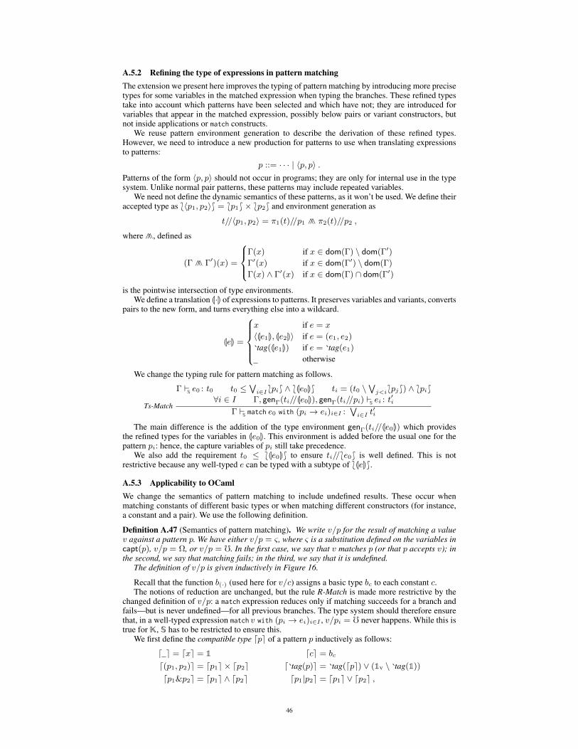
A.5.2 Refining the type of expressions in pattern matchingThe extension we present here improves the typing of pattern matching by introducing more precisetypes for some variables in the matched expression when typing the branches. These refined typestake into account which patterns have been selected and which have not; they are introduced forvariables that appear in the matched expression, possibly below pairs or variant constructors, butnot inside applications or match constructs.

We reuse pattern environment generation to describe the derivation of these refined types.However, we need to introduce a new production for patterns to use when translating expressionsto patterns:

p ::= · · · | 〈p, p〉 .Patterns of the form 〈p, p〉 should not occur in programs; they are only for internal use in the typesystem. Unlike normal pair patterns, these patterns may include repeated variables.

We need not define the dynamic semantics of these patterns, as it won’t be used. We define theiraccepted type as *〈p1, p2〉+ = *p1+× *p2+ and environment generation as

t//〈p1, p2〉 = π1(t)//p1 ∧∧ π2(t)//p2 ,

where ∧∧, defined as

(Γ ∧∧ Γ′)(x) =

Γ(x) if x ∈ dom(Γ) \ dom(Γ′)

Γ′(x) if x ∈ dom(Γ′) \ dom(Γ)

Γ(x) ∧ Γ′(x) if x ∈ dom(Γ) ∩ dom(Γ′)

is the pointwise intersection of type environments.We define a translation L·M of expressions to patterns. It preserves variables and variants, converts

pairs to the new form, and turns everything else into a wildcard.

LeM =

x if e = x

〈Le1M, Le2M〉 if e = (e1, e2)

tag(Le1M) if e = tag(e1)

otherwise

We change the typing rule for pattern matching as follows.

Ts-Match

ΓSe0 : t0 t0 ≤

∨i∈I*pi+ ∧ *Le0M+ ti = (t0 \

∨j<i*pj+) ∧ *pi+

∀i ∈ I Γ, genΓ(ti//Le0M), genΓ(ti//pi) Sei : t

′i

ΓSmatch e0 with (pi → ei)i∈I :

∨i∈I t

′i

The main difference is the addition of the type environment genΓ(ti//Le0M) which providesthe refined types for the variables in Le0M. This environment is added before the usual one for thepattern pi: hence, the capture variables of pi still take precedence.

We also add the requirement t0 ≤ *Le0M+ to ensure ti//*e0+ is well defined. This is notrestrictive because any well-typed e can be typed with a subtype of *LeM+.

A.5.3 Applicability to OCamlWe change the semantics of pattern matching to include undefined results. These occur whenmatching constants of different basic types or when matching different constructors (for instance,a constant and a pair). We use the following definition.

Definition A.47 (Semantics of pattern matching). We write v/p for the result of matching a valuev against a pattern p. We have either v/p = ς , where ς is a substitution defined on the variables incapt(p), v/p = Ω, or v/p = f. In the first case, we say that v matches p (or that p accepts v); inthe second, we say that matching fails; in the third, we say that it is undefined.

The definition of v/p is given inductively in Figure 16.

Recall that the function b(·) (used here for v/c) assigns a basic type bc to each constant c.The notions of reduction are unchanged, but the rule R-Match is made more restrictive by the

changed definition of v/p: a match expression reduces only if matching succeeds for a branch andfails—but is never undefined—for all previous branches. The type system should therefore ensurethat, in a well-typed expression match v with (pi → ei)i∈I , v/pi = f never happens. While this istrue for K, S has to be restricted to ensure this.

We first define the compatible type dpe of a pattern p inductively as follows:

d e = dxe = 1 dce = bc

d(p1, p2)e = dp1e × dp2e d tag(p)e = tag(dpe) ∨ (1V \ tag(1))

dp1&p2e = dp1e ∧ dp2e dp1|p2e = dp1e ∨ dp2e ,

46

v/ = [ ]

v/x = [v/x]

v/c =

[ ] if v = c

Ω if v ∈ C, bv = bc, and v 6= c

f otherwise

v/(p1, p2) =

ς1 ∪ ς2 if v = (v1, v2) and ∀i. vi/pi = ςiΩ if v = (v1, v2), ∃i. vi/pi = Ω, and ∀i. vi/pi 6= ff otherwise

v/ tag(p1) =

ς1 if v = tag(v1) and v1/p1 = ς1Ω if v = tag(v1) and v1/p1 = Ω or if v = tag1(v1) and tag1 6= tagf otherwise

v/p1&p2 =

ς1 ∪ ς2 if ∀i. v/pi = ςiΩ if ∃i. v/pi = Ω and ∀i. v/pi 6= ff otherwise

v/p1|p2 =

v/p1 if v/p1 6= Ω

v/p2 otherwise

Figure 16. Semantics of pattern matching including undefined results.

where 1V is the top type for variants, defined in Section 4.3, Footnote 5. For all well-typed valuesv, Γ

Sv : dpe holds if and only if v/p 6= f.

We change the rule for pattern matching by requiring the type t0 we assign to the matchedexpression to be a subtype of all compatible types dpie.

Ts-Match

ΓSe0 : t0 t0 ≤

∨i∈I*pi+ ∧

∧i∈Idpie ti = (t0 \

∨j<i*pj+) ∧ *pi+

∀i ∈ I Γ, genΓ(ti//pi) Sei : t

′i

ΓSmatch e0 with (pi → ei)i∈I :

∨i∈I t

′i

Note that this condition is somewhat more restrictive than necessary: patterns which follow acatch-all (wildcard or variable) pattern—or in general that are useless because previous patternsalready cover all cases—can be left out of the intersection. The precise condition would be

t0 ≤∨i∈I

(*pi+ ∧

∧j<idpje

),

but we choose the simpler condition since they only differ in case there is redundancy.

47