Setting Environmental Standards: A Statistician's Perspective

Peter Guttorp

NRCSE T e c h n i c a l R e p o r t S e r i e s

NRCSE-TRS No. 048

May 31,2000

The NRCSEwas established in 1996 through a cooperativeagreement with the Uniled States Environmental Protection Agency which provides the Center's primary funding.

1. Introduction

In order to protect the population from adverse health effects due to pollution of air, water and soil, many governments choose to set a standard, i. e., a value (such as daily average concentration of a particular pollutant) not to be exceeded, or to be exceeded only infrequently. In addition to the standard, an implementation rule, indicating under what circumstances the standard will be considered violated, is usually part of the regulations. Finally, penalties and other procedures for dealing with regions out of compliance with the standard may also be part of the legislation.

In this paper we consider the US national ambient air quality standards (NAAQS), and particularly the standard for ozone. Due to a complicated legal issue, there are currently two ozone standards in effect, but we focus here on the older one. This standard requires states to maintain an air quality such that the expected annual number of maximum hourly averages exceeding 0.12 ppm is equal to or less than one. The implementation rule allows the state no more than three daily maximum hourly average measurements in excess of 0.12 ppm during three years at each approved monitoring site. Finally, the consequences ofviolating the standard depend on the severity of the noncompliance: if the measurements placing the state out of compliance exceed 0.18 ppm, the state must develop a comprehensive air quality model, demonstrate that the model can reproduce current data, and develop a plan for air quality improvement which, according to the model, eventually will put the state in compliance.

Previous work looking at statistical aspects of environmental standards include Watson and Downing (1976), O'Brien et al. (1991), Symon et al. (1993), Barnett and O'Hagan (1997). Cox et al. (1999) and Carbonez et al. (1999). This paper is structured as follows. In section 2 we give a statistician's first approach to the problem of determining compliance with the ozone standard. In section 3 we analyze in a similar fashion the implementation rule of the United States Environmental Protection Agency (EPA). Section 4 has some data analyses from different parts of the United States, and a discussion of the validity of the simplifying assumptions made in sections 2 and 3. A statistical framework for setting environmental standards have been developed by Barnett and O'Hagan (1997), and we outline how this can be applied to the US ozone standard in section 5. Finally, in section 6 we look at the potential bias of using compliance monitoring networks to assess health effects of air pollution.

2. A statistical setup

Consider a monitoring network with I sites, and let Ni,, denote the number of daily maximum hourly averages in excess of 0.12 ppm at site i, i= 1,...,I, during year t,

?=I,...,T. Let Bi = For simplicity, let us first consider the case IE Ni,,. = 1.Then the

standard requires that 8 , I1. A natural approach (at least for a classically schooled statistician) to the decision as to whether the standard has been met is a hypothesis test. Since the Clean Air Act (CAA) requires the EPA first and foremost to protect people from adverse health effects of air pollution, the more serious error would be to declare a region in compliance when it is not. Hence the null hypothesis must be that of noncompliance, i.e., testing

H,: e > 1

against

Assume now that different days of the year are independent. If the monitoring site lies on the boundary between the null and alternative hypotheses, i.e., has 8 = 1, we

would have N],, - Bin(365, 11365). If we, as the EPA implementation rule requires, base

the decision on T = 3 years of data, we have N,,, -Bin(3 -365, 11365) or, to a very good approximation, Po(3). The optimal test (Rao, 1973, section 7a) is to reject for small

values of N,,, ,and a level 0.05 test rejects only if N,,, = 0. In other words, from the Neyman-Pearson testing point of view, any exceedance of 0.12 ppm during a three-year period would render a site in violation of the standard.

Considering now I independent sites, sufficiency suggests basing a test on

~ I , N , , ,Po(31). Again, the test would reject for small values of the test statistic, N.,, =

chosen so that P(N.,, 5 C,,,) I a.

In this analysis we have made (at least) three simplifying assumptions: that Ni,, is an observable random variable, that subsequent days are independent, and that different sites in the state are independent. We discuss these assumptions in section 4.

3. The EPA compliance criterion

Following the same line of thought as in the previous section, we first consider the EPA implementation rule for a single site in a state. The rule declares a site in

compliance whenever N1,3< 3, which when 0 = 1 has probability a= 0.647 under the

assumption of consecutive daily maxima being independent. As no statistician would even consider values of a this high, one may argue that the EPA are not performing their

mission under the CAA: given that the CAA requires the EPA to protect public health, and that the agency has decided that 0.12 ppm maximum daily hourly average is a limit above which serious health risks to the public occur, the agency appears to make type I errors much too frequently under their implementation rule.

One naturally wonders how this implementation rule was arrived at. The explanation in the regulation (Title 40 of US Code of Federal Regulations part 50, Appendix H) says:

The ozone standard states that the expected number of exceedances per year must be less than or equal to 1. The statistical term "expected number" is basically an arithmetic average. The following example explains what it would mean for an area to be in compliance with this type of standard. Suppose a monitoring station records a valid daily maximum hourly average ozone value for every day of the year during the past 3 years. At the end of each year, the number of days with maximum hourly concentrations above 120ppb is determined and this number is averaged with the results of previous years. As long as this average remains "less than or equal to 1," the area is in compliance.

In other words, this section of the United States Code requires the law of large numbers to be applied to n = 3.

For a region with more than one site, the EPA implementation rule uses the test

statistic T, = maxi,, N,,,,again rejecting H,,if TI5 3. For example, assuming again

spatially independent sites, we find for I= 7 that a = 0.05. The corresponding rule from

section 2 would be to reject when N.,3I13, regardless of where in the network the

violations have taken place. It should be noted here that the calculation is made assuming that all the sites have 0 = 1, so it would be quite unlikely, for example, that one site

would have 13 violations and all the other none. In fact, using a simple multinomial calculation, with a frequency of about 0.36 the maximum number of violations at any of the seven sites, given that 13 violations occurred, would be three, so both implementations agree about 113 of the time.

4. Data analysis

In this section we consider data from three heavily polluted regions in the United States: the Chicago area in Illinois, the South Coast region of California, and the Houston area in Texas. Previous analyses (e.g., Carroll et al., 1998; Cox et al., 1999) have indicated that a square root transformation frequently has the effect of symmetrizing the ozone data, making a Gaussian assumption reasonable. The data are available from the AIRS data base (Chicago and Houston; http://www.epa.gov/airs) and from the California Air Resources Board (South Coast California; http://www.arb.ca.gov/homepage.htm). Table 1 contains summary statistics for the three data sets. The EPA defines the ozone season to be the entire year in California and Texas, and April 1-October 31 in Illinois.

***Table 1 about here***

If the square root of ozone has a Gaussian distribution with mean p and standard deviation o we have that

P(exceedance of level c) = 1-cD -(Jc; p,

Using the standard deviation for the Houston network, a simple Gaussian calculation shows that one expected exceedance (for a single station) would correspond to a mean of 0.146 on the square root scale, or about 0.022 ppm on the raw scale. Hence, in order to bring Houston into compliance, the average daily maximum hourly readings must be reduced by a factor of three, from the current average of 0.066 ppm. Of course, corrective action that reduces only high readings may also be possible.

The considerations so far in this paper have all assumed (at least implicitly) that the

quantity N,,,is an observable random variable, i.e., that we can determine without error the number of exceedances of a given level at a site from the measured daily maximum hourly ozone averages. This is not strictly speaking the case, since the measurements are made with error. In order to take this into account, we need to make a conditional calculation. Assume for simplicity a Gaussian additive measurement model on the square root scale, namely Y = Z + E, where Y is the observed square root daily maximum hourly

ozone average, Z is the square root of true maximum daily hourly ozone average, assumed N(p, 02), and E an independent measurement error, assumed N(0,z2). Here o2 corresponds to the natural variability of the ozone field, and zZ to the uncertainty due to

imprecise measurement techniques. Then we have, using a standard regression calculation for'the case p = a,that

where A2=(52/~2i~ the signal-to-noise ratio. This corresponds to increasing the standard

deviation of the underlying pollution field by a factor of (E- I)-'.

The analysis in Cox et al. (1999) for California Central Valley data indicates that the standard deviation 7 of the measurement errors for common instruments are about

0.020-0.027 on the square root ppm scale, corresponding to a error standard deviation of the raw measurements of about 0.002-0.003 ppm at a mean level of 0.12 ppm. Comparing these values to those in Table 1 indicates that the measurement error is a fairly large proportion of the observed variability. Using ~~=0.00041 and 02=0.00381,

corresponding to the South Coast California data, we get the multiplier (n-1)

equal to 2.19. Figure 1 shows the conditional probability, given an observation of y, that the true field actually is above 0.12 ppm. In order for this probability to be bigger than 0.95, we need an actual reading of at least 0.156 ppm.

***Figure 1 about here ***

The assumption of iid data is overly simplistic. First, i t fails to take into account the seasonal distribution of ozone, which is very pronounced in the data we consider in this paper. For example, in the California Southern Coast data the ozone levels are lower in the winter and higher in the summer. This can be taken care of in a more realistic fashion by using time-varying mean and variance. More seriously, perhaps, is the fact that the time series of daily maximum hourly average ozone show some autocorrelation. Data analysis indicates that an AR(2)-model can take care of most of the autocorrelation. The calculations for single station exceedances can be redone, using simulation techniques, for a more realistic model.

Finally, we need to consider the spatial correlations. In the Chicago data set, the site- to-site correlations are 0.7 or higher. Hence, the calculations earlier in the paper assuming spatially independent stations are not valid for the Chicago network. Simulation studies, matching the distribution of hourly maxima over the network with independent hourly maxima indicate that the 10-station networks correspond to about two independent

stations. Hence, regional spatially expressed standards would be preferable to the current formulation.

5. The Barnett-O'Hagan setup

In a report written for the Royal Commission on the Environment in the UK, and subsequently published as a book, Barnett and O'Hagan (1997) developed a framework for the statistical implementation of environmental standards. They distinguished between ideal standards, setting limits on the true pollution field, and realizable standards, set in terms of actual measurements. Ideal standards (the US ozone standard is an example) are a natural approach to standard setting, in that they can be related to or even based on the scientific evidence regarding health effects, crop damage, etc. On the other hand, it is impossible to implement an ideal standard. In the US ozone case, we cannot measure the number of exceedances everywhere in the state, much less measure the expected value of this random variable. Thus, realizable standards are much easier to implement (both politically and practically), since they specify exactly what measurements constitute a violation of the standard. The downside is that it is very difficult to relate a realizable standard to the actual pollution field and consequent health effects.

It is natural to seek a compromise between these two extremes. Barnett and O'Hagan suggest a statistical implementation of an ideal standard, in their terminology a statistically verifiable ideal standard. In the case of the US ozone standard, this amounts to specifying statistical quality parameters for deciding whether a given region is in compliance with the standard. In the testing setup, a natural approach is to fix the type I and type I1 errors, the former at a value beyond which health effects are serious, and the latter at a value for which there is no evidence of health effects, or at a value corresponding to peak background levels.

6. Network monitoring bias

The states are responsible for monitoring compliance with the standards in the CAA. To this effect, they operate monitoring networks, which have to be approved by the local EPA authorities. Since the network is primarily aimed at finding large values of air pollution, a site that consistently shows lower values than another is likely to be closed down. Hence, the monitoring network setup keeps changing over time, with sites selected based on high values rather than in a random or systematic fashion. In this section, we

illustrate the potential bias in a network using a very simple space-time model for air pollution.

Suppose X, = AX, ,+ %is a stationary vector time series, mean p,with E, - N(0,Z)

where 2 has diagonal elements one, and off-diagonal elements oij= p, iitj, i.e., an

exchangeable spatial process. The spatial structure of some of the ozone data mentioned in the previous section can be reasonably described by this correlation structure. Also assume that A = diag (a,, ...a,). A simple Gaussian calculation shows that

Defining the network bias as the excess over the mean k,,given that during the previous time period site 1 was chosen and site 2 deleted on the basis of the former site having a higher reading than the latter, we see that the autoregressive parameter a,is the main contributor to a potential network bias. The largest bias occurs for high temporal correlation and negative spatial correlation (an unlikely situation for air pollution data), with a maximum bias of 0.40 standard deviations. The autocorrelation is generally decreasing with larger temporal scale, so one would not expect the bias to be substantial on an annual time scale in this very simple model. Research continues into what can be expected in long term memory processes (Beran, 1997), where the autocorrelation dies off very slowly with time. These types of models have been found appropriate, e.g., for some temperature data (Smith, 1992).

The consequence of using compliance monitoring networks to study health effects can be serious even in absence of the bias discussed above. Most health effect studies (see e.g., Thomas, 2000) take the ambient measurements closest to an individual's home andlor workplace as a surrogate for exposure. Clearly, if the ambient concentration measurements are from data chosen to find peaks in the mean spatial field, the exposure of an individual will be overestimated, resulting in an underestimate of the health effects of exposure to a given level of pollution. This is a potentially very serious bias, particularly since the relative risk estimates in environmental epidemiology often are close to 1. Studies using personal monitors may be helpful in order to assess more precisely the health effects of a given exposure. Current technology, however, produces rather unwieldy monitors, which are likely to affect personal behavior.

Acknowledgements

Although the research described in this article has been funded in part by the United States Environmental Protection Agency through agreement CR825173-01-0 to the University of Washington, it has as not been subjected to the Agency's required peer and policy review and therefore does not necessarily reflect the views of the Agency and no official endorsement should be inferred. The author is grateful to the NRCSE standards group, in particular Mary Lou Thompson, Larry Cox and Paul Sampson, for lots of illuminating discussions, and Anthony Nguyen for computational help.

References

Barnett. V. and O'Hagan, A. (1997): Setting environmental staildards: the statistical approach to handling uncertainty and variation. London: Chapman &Hall.

Beran, J. (1997): Statistics For Long-Memory Processes. New York: Chapman & Hall.

Carbonez ,A., El-Shaarawi, A. H. and Teugels, J. L. (1999): Maximum microbioIogical contaminant levels. Environmetrics 12: 79-86.

Carroll, R. J., Chen, R., George, E. I., Li, T. H., Newton, H. J., Schmiediche, H. and Wang, N. (1997): Trends in ozone exposure in Harris County, Texas. J.Amer. Statist. Assoc. 92: 392-415.

Cox, L. H., Guttorp, P., Sampson, P. D., Caccia, D. C. and Thompson, M. L. (1999): A preliminary statistical examination of the effects of uncertainty and variability on environmental regulatory criteria for ozone. In Novartis Foundation Symposium 220, Environnzental Statistics: Artalysing Data for Environnzerttal Policy, pp. 122-143. Chichester: Wiley.

O'Brien, W., Sinha, B. K. and Smith, W. P. (1991): A statistical procedure to evaluate cleanup standards. J. Chemometrics5: 249-261.

Rao, C. R. (1973): Linear Statistical Inference and its Applications. 2" ed. New York: Wiley.

Smith, R. L. (1992): Long-range dependence and global warming. In V. Bamett and K. F. Turkman (eds.): Statistics for the Environment, pp. 141-161. Chichester: Wiley.

Symons,M. J., Chen, C.-C., and Flynn, M. R. (1993): Bayesian nonparametrics for compliance to exposure standards. J. Amer. Statist. Assoc. 88: 1237-1240.

Thomas, D. C. (2000): Some contributions of statistics to environmental epidemiology.J.Amer. Statist. Assoc. 95: 315-319.

Watson, W. D. and Downing, P. B. (1976): Enforcement of environmental standards and the central limit theorem. J. Amer. Statist. Assoc. 71:567-573.

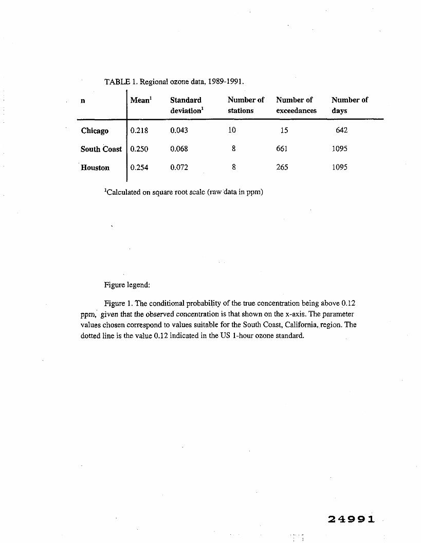
TABLE 1. Regional ozone data, 1989-1991.

n Mean' Standard Number of Number of Number of deviation1 stations exceedances days

Chicago 0.218 0.043 10 15 642

South Coast 0.250 0.068 8 661 1095

Houston 0.254 0.072 8 265 1095

'Calculated on square root scale (raw data in ppm)

Figure legend:

Figure 1. The conditional probability of the true concentration being above 0.12 ppm, given that the observed concentration is that shown on the x-axis. The parameter values chosen correspond to values suitable for the South Coast, California, region. The dotted line is the value 0.12 indicated in the US 1-hour ozone standard.